Ultra Fast Astronomy: Optimized Detection of Multimessenger Transients

Abstract

Ultra Fast Astronomy is a new frontier becoming enabled by improved detector technology allowing discovery of optical transients on millisecond to nanosecond time scales. These may reveal counterparts of energetic processes such as fast radio bursts, gamma ray bursts, gravitational wave events, or play a role in the optical search for extraterrestrial intelligence (oSETI). We explore some example science cases and their optimization under constrained resources, basically how to distribute observations along the spectrum of short duration searches of many targets or long searches over fewer targets. As a demonstration of the method we present some analytic and some numerical optimizations, of both raw detections and science characterization such as an information matrix analysis of constraining a burst delay – flash duration relation.

1 Introduction

The transient sky is a treasure trove (Wyatt et al., 2020) of events and information about the energetic universe, ranging over gamma ray to radio wavelengths in light, plus neutrinos and gravitational waves, and over time scales from milliseconds to months. Well known cosmological examples include fast radio bursts (FRB) and gamma ray bursts (GRB) on millisecond to second timescales, binary black hole inspiral gravitational waves over milliseconds to days, and supernovae over days to months. Of course the entire universe can be viewed as transient over long enough timescales (Stebbins, 2012; Erskine et al., 2019; Kim et al., 2015; Marcori et al., 2015; Bel & Marinoni, 2018; Quercellini et al., 2012).

Time domain surveys specifically seek to explore the transient sky, with the next generation coming underway (Bellm et al., 2019; Mandelbaum et al., 2018). Continuously scanning surveys can also detect transient events (Naess et al., 2021; Abazajian et al., 2019; Slosar et al., 2019; Whitehorn et al., 2016). Multimessenger detection of an event in photons of diverse wavelengths, other high energy particles such as neutrinos or cosmic rays, or gravitational waves is a burgeoning new field, e.g. Kalogera et al. (2019); Dyer et al. (2012); Hallinan et al. (2019); Blakeslee et al. (2019); Kasliwal et al. (2019). However, all these surveys tend to scan over seconds to days, insensitive to transients on shorter timescales (but see Arimatsu et al. (2021); Yang et al. (2019); Shearer et al. (2010)). Certainly we know that astrophysical energetic events can occur down to nanosecond timescales, e.g. Philippov et al. (2019); Stebbins & Yoo (2015). If optical and ultraviolet, infrared, etc. surveys sensitive to subsecond timescales can be realized, might they reveal a whole new world of events at cosmological distances?

Detector technology and imaging software is reaching capabilities to make such surveys a reality. In particular, the development of silicon photomultiplier arrays (SiPM) with ultrafast readout and coincidence triggers (Lau et al., 2020; Li et al., 2019b) may open up the era of Ultra Fast Astronomy, on millisecond and even submicrosecond timescales in the optical and near infrared. Other detectors such as avalanche photodiodes (Li et al., 2019a) are also being explored. While they still have a long way to go in terms of large arrays, spatial resolution, and noise including crosstalk, they are capable of single photon detection and continuous readout.

The discovery of optical millisecond and below transients would be a major breakthrough, rife with astrophysical information and numerous applications. Here we focus on one particular aspect of this new field of Ultra Fast Astronomy: transients visible in multiple windows, e.g. gamma rays and optical light, or gravitational waves and optical light, that can be targeted, i.e. there is a precursor or repeating event. That is, we specifically seek connections with known – or yet to be found – ultra fast transients. Examples include the search for optical counterparts of known energetic events, such as repeating fast radio bursts (FRB), delayed optical phenomena from a one time event, or even as part of an optical search for extraterrestrial intelligence (oSETI) program (Wright et al., 2018; Kipping & Teachey, 2017; Davenport, 2019).

The size of detectors arrays, the possible field of view, and the instrumental characteristics are yet unknown. What we aim for here is merely to give a flavor of the science investigations and methods that might prove useful. Of necessity these will need to be adjusted for specific situations, e.g. particular types of bursts to follow, instrument properties, etc. However the general optimization framework we present should be a good guiding tool, regardless of the specific burst properties used as toy examples.

Framed generally: given a set of adaptable observations, a merit function to optimize, a limited resource, and a cost function per observation, what is the best strategy for achieving some science characterization. Our main topic of investigation will be ways of optimizing a detection or characterization of an astrophysical process given a large set of targets (e.g. prior burst locations) but limited observing resources – e.g. how much time should be spent on each target to best achieve the proposed goal. We emphasize that this is in essence a follow up program; we assume a target list of interesting objects, e.g. repeating FRB, exists and we seek detection of optical transients from them.

Astrophysically, such an optimization analysis has been carried out for strong gravitational lens surveys (Linder, 2015) and supernova surveys (e.g. Huterer & Turner (2001); Frieman et al. (2003)). For example there the optimization was for the data set distribution, the number of targets followed up at different redshifts, while the merit function was the dark energy joint parameter estimation uncertainty (“figure of merit”), the limited resource was the total spectroscopy time, and the cost function expressed the resource use of followup spectroscopic time by a target at redshift $z$. There may also be a systematics function that effectively caps the number of useful targets in each observation (e.g. redshift) bin.

To develop and demonstrate the method we explore three separate science approaches. We emphasize that these are only toy examples; applications of Ultra Fast Astronomy are likely to be much richer and more varied, and of course instrumental specifics will play a much larger role. In Section 2 we describe the basic foundation, in terms of a target source (known for repeating or predictable bursts) and its possible optical counterparts – here called flashes. Section 3 demonstrates the optimization procedure on the question of how to allocate limited observing time if one wants to use flash abundances to connect flash properties to burst characteristics. A more physically incisive test of a property such as a burst delay – flash duration relation, possibly useful as a test of oSETI, is optimized in Section 4 when using measurements of flash durations rather than mere abundances. Such examples should give the flavor, and potential exciting promise, of the general approach. We discuss further potential opportunities from technology development and conclude in Section 5. In the Appendix A we present some analytic results on maximizing detections by considering basic two or three time bin optical followup programs of repeating bursts, just using this simple example to illustrate some general principles of resource constrained optimization.

2 Burst optical counterparts

The basic idea is that there is a list of targets for which we seek to detect optical transients. In particular, we consider the targets to be sources that burst in some other wavelength, and we look for optical counterparts. One example might be fast radio bursts we follow up with an optical program to look for ultra fast optical transients. This phrasing is purely a matter of convenience and indication of an interesting science goal, without drawing on specific FRB properties – the principles are kept generally applicable. Fast radio bursts are millisecond transients detected at radio wavelengths (Petroff et al., 2019). A fraction of them repeat, though not necessarily periodically. They may, however, have “active windows” that are periodic, with enhanced probability of a repeat burst sometime within the window; this has also been detected for soft gamma repeaters (Denissenya et al., 2021).

The optical program is thus essentially a followup program, scanning targets that have previously burst, not a blind survey. We distinguish the transients by saying that we look for flashes (e.g. in optical) that are targeted on previous bursts (e.g. in radio) – and in particularly targeted at a time when we have some reason to expect a repeat burst so that we can look for coincident, or nearly coincident, flashes and bursts. (Also, active windows for bursts do not always deliver actual activity, but it is possible there may be activity of interest at that time in other wavelengths.)

Determining whether FRB, or any other bursting sources, have optical emission, and measuring it, would be important for understanding the physics behind the source; so far the millisecond timescale is too short to make such optical (or UV or NIR) observations. As initial goals of Ultra Fast Astronomy we might seek to maximize the chances of detecting an optical counterpart, i.e. the numbers of such burst counterparts, and to learn some basic physics behind the flash. We discuss these in Section 3 and Section 4 respectively.

The first step to investigate the relation between flashes and bursts is take a probability for a burst within an observing window and propagate it to the number of flashes over a distribution of observing times, i.e. a survey. Suppose the probability distribution function (PDF) of a burst repeating a time $t$ after a previous burst (so we know where to look) and having an optical counterpart (so there is something to detect) is some normalized $p_{\rm burst}(t)$. Then in a window of time $[t_{i-1},t_{i}]$ the probability of a viable repeat burst is

$$p_{i}(t_{i})=\int_{t_{i-1}}^{t_{i}}dt\,p_{\rm burst}(t)\,.$$ (1)

This may be a function of burst properties, and we may later be interested in subtypes, but for now we simply consider any burst.

Our basic question is whether we want a quick look at many targets or a long look at fewer targets – what is the optimum allocation? The observing procedure is taken to be assignment from a target list to observing times of various durations. For example, some targets we will observe for a duration $t_{1}$ and if no flash is detected we move on to another target. Some targets we will observe for $t_{2}$ – if it does not flash by time $t_{2}$ we move on, if it flashes in the first $t_{1}$ time then we do not continue to observe it afterward, and instead assign it to the $t_{1}$ “bin”, and if it flashes between times $t_{1}$ and $t_{2}$ then it is in the bin corresponding to $t_{2}$, etc. We consider an ordered set of discrete times $t_{i}$, where $t_{i}>t_{i-1}$ and $t_{0}=0$. This is both for mathematical simplicity and because of the possibility that instrumental constraints may impose certain intervals. One could redo the calculations with finer divisions; this does not affect the overall principle. The target list should be viewed as locations of interest; we do not know exactly when the next event will occur, certainly not on the subsecond time scale of the transients. Unlike a rolling search for supernova explosions, say, where we target a set of galaxies, while supernovae will stay visible for a month or more, bursts go undetected if we are not already observing their location.

The number of flashes detected is

$$N_{\rm flash}=\sum_{i}N_{\rm target}(t_{i})\,p_{i}\equiv\sum_{i}n_{i}p_{i}\,,$$ (2)

where $n_{i}\equiv N_{\rm target}(t_{i})$ is the number of targets with observation duration $t_{i}$ (i.e. producing, or not, a flash between $t_{i-1}$ and $t_{i}$). Again the question we focus on is what is the optimum allocation $n_{i}(t_{i})$ – do we want a quick look at many targets or a long look at fewer targets? (The following calculations assume a single burst population; at the end of Section 4 we explore multiple source populations, corresponding to an extra summation index in Eq. 2 for example.)

A further real world complication is limited resources, e.g. telescope time, meaning that we cannot observe as many targets as we want for as long as we want. Each observation comes with a cost, taking up part of finite resources $R$. The cost function may be simply proportional to observing time, i.e. how much time we dedicate to searching for a flash from a target, so

$$R=\sum_{i}n_{i}t_{i}\,.$$ (3)

Here we take all times, and $R$, to be in units of $t_{1}$, the shortest observation time. That may be one second, one day, or whatever; that will depend on the specific target population and instrument, but we leave that for future detailed survey design. Given detailed instrument and survey design, the observing procedure can be further adjusted by employing Monte Carlo methods taking into account, e.g., telescope slew and readout times (see the discussion on such issues at the end of Section 4). We also emphasize that at this stage we are not aiming for a complete survey, detecting all counterparts, but rather a reasonable attempt at an initial set of counterpart flashes.

3 Delay-Duration Relation – via Abundance

While detecting ultra fast optical transient counterparts would be exciting and significant, it would be even better to extract some physics out of the detections. We consider the following as one illustration. Suppose the optical flash durations $\tau$ are connected with the burst repeat delay time $t_{p}$ through a power law scaling. We write

$$\tau=At_{\star}\,\left(\frac{t_{p}}{t_{\star}}\right)^{s}\,,$$ (4)

where $t_{\star}$ is a fixed pivot scale, $A$ is the dimensionless amplitude of the relation (with a $t_{\star}$ out front for correct dimensionality) and $s$ is the slope relating the mean burst delays to the flash durations. This could be relevant to the astrophysical bursting mechanism, e.g. of FRB or GRB, and also to oSETI, where a civilization might choose to broadcast short messages frequently, or long messages infrequently, in a sort of constant energy output ($s=1$) schema. We would like to test such an assumption, e.g. is $s\neq 0$ so there is a relation between the burst delay $t_{p}$ and the flash duration $\tau$, and characterize it – what estimates of amplitude $A$ and slope $s$ do we obtain from data.

We will use an information matrix approach to determining the physical parameters $A$ and $s$ from the flash detections, and then optimizing the observation time distribution to get the best constraints. In this section we take the observable to be the number of flashes in a certain observation time bin $t_{i}$, summed over the flash durations $\tau$. We want to relate these measured abundances to the underlying process parameters of the delay-duration amplitude $A$ and slope $s$. (In Section 4 we take a more direct approach, using the flash durations themselves.)

We begin with the number of flashes with duration $\tau$ detected from all bursts observed with observation time duration in bin $i$: $t_{i-1}<t_{\rm obs}<t_{i}$. A subscript $i$ means such a time bin and we take all bins to be of equal, unit width. Then

$$N_{\rm flash}(t_{i};\tau) = n_{\rm burst}(t_{i})\,p_{\rm flash}(t_{i};\tau)$$ (5)

$$= n_{\rm burst}(t_{i})\,\,p_{\rm flash}(t_{i};t_{p})\,\left|\frac{dt_{p}}{d\tau}\right|\,,$$ (6)

where we used $p_{\rm flash}(t_{i};\tau)d\tau=p_{\rm flash}(t_{i};t_{p})dt_{p}$. The quantity $p_{\rm flash}(t_{i};t_{p})$ is taken to be the probability of the repeat burst within the observing time, i.e. Eq. (1), times some probability for having a flash associated with a burst, $p_{\star}$. We set $p_{\star}=1$ for simplicity; a constant $p_{\star}$ does not affect the form of our results.

We consider a Gaussian delay model where

$$p_{\rm burst}(t)=\frac{1}{\sqrt{2\pi\sigma^{2}}}\,e^{-(t-t_{p})^{2}/(2\sigma^{2})}\,.$$ (7)

This represents a burst that occurs a mean time $t_{p}$ after time zero (e.g. the previous burst or the beginning of an activity window), but with some uncertainty $\sigma$. While this is just a model, it is a reasonable first choice; one would need to determine the burst delay distribution in the process of building up the target list. The probability for a flash within a window $[t_{i-1},t_{i}]$, and hence being assigned to observation duration $t_{i}$, is then

$$p_{i}(t_{i})=\frac{1}{2}\,\left[{\rm erf}\left(\frac{t_{i}-t_{p}}{\sigma\sqrt{2}}\right)-{\rm erf}\left(\frac{t_{i-1}-t_{p}}{\sigma\sqrt{2}}\right)\right]\,.$$ (8)

This gives all the necessary ingredients for the calculation. Using the inverse of Eq. (4),

$$t_{p}=t_{\star}\,\left(\frac{\tau}{At_{\star}}\right)^{1/s}\,,$$ (9)

we can calculate the Jacobian

$$J\equiv\left|\frac{dt_{p}}{d\tau}\right|=\frac{1}{As}\,\left(\frac{\tau}{At_{\star}}\right)^{(1-s)/s}\,.$$ (10)

Explicitly,

$$N_{\rm flash}(t_{i};\tau) = n_{\rm burst}(t_{i})\,\,p_{\rm flash}(t_{i};t_{p}(\tau,A,s))$$ (11)

$$\times\frac{1}{As}\left(\frac{\tau}{At_{\star}}\right)^{(1-s)/s}\,.$$

To carry out the information analysis, we need the sensitivities: the derivatives with respect to the parameters,

$$\frac{\partial N_{\rm flash}(t_{i},\tau)}{\partial A}\,,\qquad\frac{\partial N_{\rm flash}(t_{i},\tau)}{\partial s}\,.$$ (12)

Note that

$$\frac{\partial p_{i}(t_{p}(\tau,A,s))}{\partial\theta}=\frac{\partial p_{i}(t_{p}(\tau,A,s))}{\partial t_{p}}\,\frac{\partial t_{p}}{\partial\theta}\,,$$ (13)

for $\theta=\{A,s\}$ and $p_{i}(t_{p})\equiv p_{\rm flash}(t_{i};t_{p})$. The derivatives

$$\frac{\partial t_{p}}{\partial A}=\frac{-t_{p}}{sA}\,,\qquad\frac{\partial t_{p}}{\partial s}=\frac{-t_{p}}{s^{2}}\,\ln\left(\frac{\tau}{At_{\star}}\right)\,,$$ (14)

and for the Jacobian factor

$$\frac{\partial J}{\partial A}=\frac{-J}{sA}\,,\qquad\frac{\partial J}{\partial s}=\frac{-J}{s^{2}}\,\left[s+\ln\left(\frac{\tau}{At_{\star}}\right)\right]\,.$$ (15)

Putting it all together,

$$\frac{\partial N_{\rm flash}(t_{i},\tau)}{\partial A}=\frac{-N_{\rm flash}}{sA}\left[\frac{t_{\star}}{p_{i}(t_{p})}\frac{dp_{i}}{dt_{p}}\left(\frac{\tau}{At_{\star}}\right)^{1/s}+1\right]\,,$$ (16)

and

$$\frac{\partial N_{\rm flash}(t_{i},\tau)}{\partial s} = \frac{-N_{\rm flash}}{s^{2}}\left[\frac{t_{\star}}{p_{i}(t_{p})}\frac{dp_{i}}{dt_{p}}\left(\frac{\tau}{At_{\star}}\right)^{1/s}\ln\left(\frac{\tau}{At_{\star}}\right)\right.$$ (17)

$$\left.+s+\ln\left(\frac{\tau}{At_{\star}}\right)\right]\,,$$

where the derivatives are evaluated at $t_{p,{\rm fid}}=t_{\star}(\tau/At_{\star})^{1/s}$. For $p_{i}(t_{p})$ given by Eq. (8), its derivative is a difference between Gaussians; note the $1/p_{i}(t_{p})$ term cancels the $p_{i}(t_{p})$ in $N_{\rm flash}$.

We also need to specify the abundance measurement noise matrix, e.g. Poisson measurement error on the abundances so that $C^{-1}=N_{\rm flash}(t_{i},\tau)$, and the fiducial values, e.g. $s=1$ and $A=1/4$, with a pivot scale $t_{\star}=40$. The information matrix is summed over the bins in $\tau$ – with the constraint that $\tau<t_{i}$ (we can’t measure a duration longer than we have observed for) – and then summed over bins in observing time $t_{i}$. Thus,

$$F_{pq} = \sum_{{\rm bins\ of\ }t_{i}}\ \sum_{{\rm bins\ with\ }\tau<t_{i}}$$ (18)

$$\quad\frac{\partial N_{\rm flash}(t_{i},\tau)}{\partial\theta_{p}}\frac{\partial N_{\rm flash}(t_{i},\tau)}{\partial\theta_{q}}\,N_{\rm flash}(t_{i},\tau)\,.$$

Figure 1 shows $N_{\rm flash}(t_{i},\tau)$ and the sensitivity derivatives $\partial\ln N_{\rm flash}/\partial\theta$ for our parameters, $\theta=A$ and $s$. We see the sensitivity curves vs the flash duration $\tau$ have very different shapes, implying little covariance is expected in their determination. Both the delay-duration amplitude $A$ and slope $s$ should be well determined if we observe a range of durations.

Figure 1: The sensitivity derivatives $\partial N_{\rm flash}/\partial\theta$ (dotted red for $s$, dashed blue for $A$) have very different shapes, i.e. dependence on the observed flash duration $\tau$, so we may expect little covariance between them, allowing both to be well estimated from data. The solid black curves show $N_{\rm flash}(t_{i},\tau)$; the dashed blue (dotted red) curves show the derivative with respect to the amplitude $A$ (slope $s$). Bolder curves are for $t_{i}=40$, thinner curves are for $t_{i}=30$.

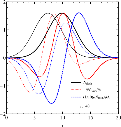
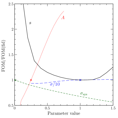
Figure 2 illustrates the information analysis results for the parameter uncertainties and the figure of merit $(\det F)^{1/2}$ related to the inverse area of the amplitude–slope confidence contour. We see that the slope is determined at about the same level for $t_{\rm obs}\gtrsim 10$ while the amplitude is best determined near the pivot scale $t_{\star}=40$. Due to the changing covariance between the parameters, however, the figure of merit (FOM) ends up being monotonic, gaining more information with a longer observation time.

Figure 2: Parameter estimation and figure of merit as a function of observing time bin $t_{i}\equiv t_{\rm obs}$. For all bins $n_{i}=10$ here.

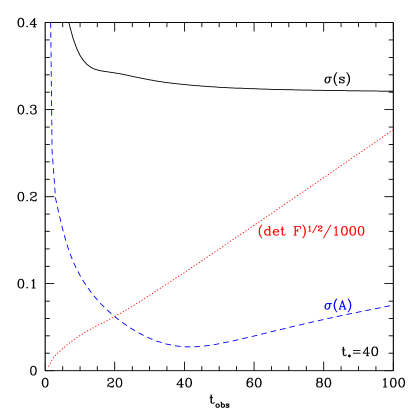
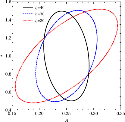
Figure 3 shows the joint $1\sigma$ confidence contours for three different values of $t_{\rm obs}$. As expected from Fig. 2, the estimation of the slope $s$ changes little, but the probability ellipse rotates to give a smaller range for amplitude $A$ near $t_{i}=40$, thinning the ellipse as $t_{i}$ increases, giving a smaller area and larger FOM.

Figure 3: Joint probability contours (68.3% confidence level) for the amplitude $A$ and slope $s$, for three different values of observing time bin $t_{i}$. For all bins $n_{i}=10$ here.

For the full information analysis, one sums over the whole range of observing time bins $t_{i}$, weighted by the number of targets in that bin, $n_{i}$. This will of course reduce the uncertainties on the parameter estimation. However our main aim is to determine the optimum observing strategy, i.e. the optimum distribution $n_{i}$, under our observing time resource constraint and cost model.

We use two independent codes to carry out the optimization. One is the information analysis optimization code described in Linder (2015), adapted for the present observables and variables, that evaluates the change in merit with resource amount (observing time), bin by bin, selects the bin with weakest leverage, reduces that $n_{i}$, and reallocates its time to other bins (hence changing $n_{j}$) in a fashion weighted by the merit per resource used. The other uses the interior point optimization algorithm which combines the resource constraint and the merit function using the barrier function approach (Weisstein, 2021). They provide valuable crosschecks on results and convergence, and we find excellent agreement between them.

The results show this optimization favors maximum numbers in the lowest observation time bin, due to the resource constraint. While FOM improves with $t_{\rm obs}$, lower $t_{\rm obs}$ allows many more targets within the given resource constraint. Since the information matrix basically goes as $n_{i}^{3}$ (two factors from the two observable $N_{\rm flash}$ proportional to $n_{i}$ and one from the Poisson noise model), putting all observations in the lowest $t_{\rm obs}$ bin wins. Of course there may be other constraints limiting the number of targets, such as from available repeaters, the telescope, detectors, etc. In that case, the optimum found fills up the lowest bin to the maximum allowed, proceeds to the next lowest bin, and so forth until the resource allotment runs out.

A short analytic proof of the behavior comes from considering the FOM if all observing is in bin $p$ vs $q>p$. In the first case, ${\rm FOM}_{1}=cn_{p}^{3}p$, where from Fig. 2 we approximate the dependence of FOM on $t_{\rm obs}$ as roughly linear. In the second case ${\rm FOM}_{2}=cn_{q}^{3}q$, but the resource constraint imposes that $n_{q}=n_{p}p/q$. Therefore we have ${\rm FOM}_{2}={\rm FOM}_{1}\,(p/q)^{2}<{\rm FOM}_{1}$ since $p<q$. Thus the lower bin always wins for this model with the abundance as the main observable.

4 Delay-Duration Relation – via Direct Measurement

The optimization in the previous section led to an all or nothing result: the solution involved flitting from target to target as fast as possible to observe as many as one could within the resource constraint. This was driven by the strong dependence of the information matrix on the number of events, due to taking the abundance as the central observable. A more subtle, and interesting, result comes if the observable is the flash duration itself, for deriving the relation to the burst delay. We analyze this case here.

The information matrix now becomes

$$F_{jk} = \sum_{t_{i}}\ \sum_{\tau<t_{i}}\frac{\partial\tau}{\partial\theta_{j}}\frac{\partial\tau}{\partial\theta_{k}}\,N_{\rm flash}(t_{i},\tau)\,C^{-1}$$ (19)

$$= \sum_{t_{i}}n_{i}\ \sum_{\tau<t_{i}}\frac{\partial\tau}{\partial\theta_{j}}\frac{\partial\tau}{\partial\theta_{k}}\,p(t_{i},t_{p}(\tau))\left|\frac{dt_{p}}{d\tau}\right|\,C^{-1}\,,$$ (20)

where $C$ is the duration measurement noise matrix. The sensitivities are

$$\frac{\partial\tau}{\partial A}=\frac{\tau}{A}\,,\qquad\frac{\partial\tau}{\partial s}=\frac{\tau}{s}\,\ln\left(\frac{\tau}{At_{\star}}\right)\,,$$ (21)

the Jacobian $|dt_{p}/d\tau|$ is given by Eq. (10), and for $C$ we take a diagonal matrix with elements $C=\sigma^{2}_{\tau}\,\delta_{qq}$ where $q$ is the index for the $\tau$ bin and

$$\sigma^{2}_{\tau}=\sigma^{2}_{\rm stat}+N_{\rm flash}(t_{i},\tau)\,\sigma^{2}_{\rm sys}\,.$$ (22)

The statistical contribution may depend on $\tau$, though here we take a fiducial case $\sigma_{\rm stat}=1$; the systematic term imposes a floor on the measurement uncertainty, or ceiling on the number of events such that increasing their quantity does not significantly add to the information beyond some limit (i.e. it cancels the $N_{\rm flash}(t_{i},\tau)$ in the numerator of $F_{jk}$: effectively, instead of a measurement uncertainty $\sigma_{\rm stat}/\sqrt{N_{\rm flash}}$ one has $\sigma_{\rm sys}$). We investigate two fiducials, $\sigma_{\rm sys}=0$ or 1, as the simplest possible examples. Real systematics would be determined by the experiment design, involving instrumentation properties related to readout, crosstalk, etc. Ultra Fast Astronomy instrumentation is not yet sufficiently advanced to yield an estimate of such systematics so we use our naive model to illustrate how it enters the optimization method we present.

We start the optimization from an initial state of uniform $n_{i}$ across all bins $t_{i}=[1,100]$, giving a fixed resource constraint of $R=5050$. Of course the survey becomes less sensitive to sources with delay times near or beyond the limit, but we want to maintain a broad survey. First we take a purely statistical uncertainty, with $\sigma_{\rm stat}=1$. Parameter estimation results will scale linearly with this, and as the reciprocal square root of the total resources available; however it will not affect the form of the distribution optimization for $n_{i}$ (for $\sigma_{\rm stat}$ independent of $\tau$). The final converged optimization gives two peaks in the $n_{i}$ target distribution, at $t_{i}\approx 6$ and 100, as seen in Fig. 4. Note Huterer & Turner (2001) also found that for a system with $P$ parameters the distribution is optimized with $P$ delta functions. The numerical solution approaches isolated peaks, with earlier iterations having slightly broader peaks, but these possess very close to the final parameter uncertainties and FOM so we see that small variations in the distribution (e.g. due to observational requirements) would have only a minor impact on the science results.

Figure 4: Histogram of the optimized target distribution $n_{i}$, producing the maximum FOM under a fixed resource constraint. The solid histograms are for a purely statistical measurement uncertainty of $\sigma_{\rm stat}=1$. Distribution results $n_{i}$ are shown for three different stages in the optimization process approaching the final convergence having sharp peaks at $t_{i}=6$ and $t_{i}=100$. Parameter constraints generally have smaller deviations from their final values than that listed for FOM. The dotted brown curve shows the impact of turning on a systematic, with $\sigma_{\rm sys}=1$, where the optimized histogram is plotted at ten times its true height (i.e. really $n_{i}<6$).

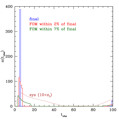
A systematic measurement uncertainty on $\tau$, given by $\sigma_{\rm sys}$, will effectively place a ceiling on the number of productive targets in a given observing bin $t_{i}$. This flattens the distribution peaks, broadening them and distributing the targets over many more bins. Including the systematics in quadrature, with $\sigma_{\rm sys}=1$, worsens the parameter estimation by 22% on $A$ and 44% on $s$, and by 33% on FOM.

We study the sensitivity of the FOM to the fiducial parameters in Fig. 5. Our fiducial value for the slope, $s=1$, is seen to be the most conservative choice: other values of $s$ give a higher FOM and tighter parameter estimation. This makes sense in that, broadly, when $s=1$ some parameter dependence does not enter, e.g. in Eq. (10) and hence $N_{\rm flash}$. More specifically, for smaller $s$ we also amplify the sensitivity $\partial\tau/\partial s$ and increase the Jacobian $dt_{p}/d\tau$. Thus we expect small $s$ to show the greatest improvement in parameter constraints and FOM. What we find for $s>1$ is that, while the parameter constraints weaken, the FOM increases since there is less covariance between parameters – this is due to the enhanced range of $\tau$ contributing to a given favored $t_{p}$ near $t_{i}$ from the $1/s$ exponent in the relation Eq. (9).

Figure 5: The change of FOM relative to the fiducial result is plotted vs the parameter values away from their fiducials (marked with x’s): $s_{\rm fid}=1$, $A_{\rm fid}=0.25$, $\sigma=10$, $\sigma_{\rm sys}=0$. To keep $\sigma$ on the same scale the x-axis is $\sigma/10$; note we cut off the curve for small $\sigma$ as it approaches the time bin width. For $A$ we cut off the curve as the flash duration approaches the burst delay time $A=1$, otherwise it would not be a flash but a continuous glow.

For the amplitude $A$, the main effect is that larger $\tau$ is preferred for a given $t_{p}$ near $t_{i}$. Since the sensitivities strengthen with increased $\tau$, and the information goes as the product of sensitivity factors, this overcomes the reduced $dt_{p}/d\tau$. In fact, since $\partial\tau/\partial s$ is the only sensitivity benefiting (with the increase in $A$ and $\tau$ canceling in $\partial\tau/\partial A$), the improvement in the estimation of $s$ and in FOM is roughly linear in $A$, while the estimation of $A$ weakens slightly. (Only FOM is shown in Fig. 5.)

Increasing the systematic $\sigma_{\rm sys}$ of course decreases FOM and worsens the parameter estimation. Even within the naive model one can get a sense, at least qualitatively, for how systematics can impact the results. The uncertainty in the burst wait time, $\sigma$, has a minor effect, since it only enters into the probability factor and not the sensitivities. Decreasing $\sigma$ makes it a little harder for $t_{i}$ to match $t_{p}$, but we can still find some $t_{i}$ matching $t_{p}$, where the probability is maximal. We have verified that varying $\sigma$ continues to produce a sharp peak at $t_{i}=7$ or slightly earlier while preserving another peak at $t_{i}=100$.

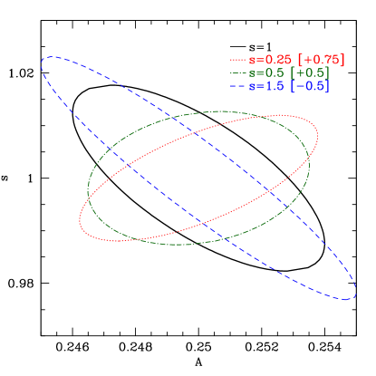
Figure 6 shows how the parameter constraints evolve as we change the fiducial slope $s$, as well as the impact on the FOM (inverse area of the confidence contour). In particular, we can see how for $s=1.5$, although the individual parameter constraints are weaker, the FOM is higher due to the narrowing of the joint contour. As the fiducial $s$ changes, the covariance between $A$ and $s$ does as well, rotating the contour and squeezing or broadening it. The slope and amplitude of the burst delay – flash duration relation can be determined at the percent level, within this model, for the resources assumed. This gives the flavor of how such a result could be promising for testing, e.g., an oSETI hypothesis of constant energy output, i.e. $\tau/t_{p}={\rm constant}$, or $s=1$. Since this plot is with statistical uncertainties only, the constraints scale with resources: linearly for FOM and as the inverse square root for the parameter estimation uncertainties.

Figure 6: $1\sigma$ joint confidence contours in the $A$–$s$ plane, for different fiducial values of $s$. Constraints are for statistical uncertainties only with $\sigma_{\rm stat}=1$. Contours have been shifted vertically by the amount in brackets so that all are centered at $s=1$, for easier comparison, despite the different fiducial values for $s$.

Finally, suppose we have multiple source populations with different properties. While the sum over flash duration $\tau$ in Eq. (20) does sum over a range of burst durations by Eq. (9), different populations may have different relations. We therefore now consider two populations, with relations having characteristics $t_{\star}=40$ or $t_{\star}=20$, and determine how the optimization changes.

Figure 7 varies the $t_{\star}=20$ population from 0% of the total (as used in the previous calculations) to 100%. We see this has very little impact on the observation duration optimization: the preferred survey still has a two peak distribution of times, one at the maximum duration and one at much shorter (but not minimum) duration. The lower peak does shift a little from $t_{\rm obs}=6$ to 7, depending on the population fraction, but we saw in Fig. 4 that the figure of merit is fairly forgiving of slight deviations from the formal optimum.

Figure 7: Histogram of the optimized target distribution $n_{i}$, producing the maximum FOM under a fixed resource constraint, for the case of two source populations. Different fractions of the source population of $t_{\star}=20$ targets relative to the full two source population of $t_{\star}=20$ and $t_{\star}=40$ targets have nearly the same optimized distribution. Here $\sigma_{\rm stat}=1$, $\sigma_{\rm sys}=0$.

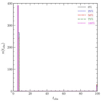
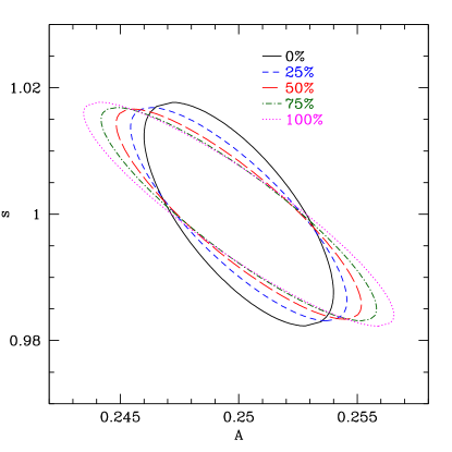
Figure 8 shows that the constraints on the parameters of the flash duration – burst delay relation do change somewhat with source population fraction. The amplitude uncertainty $\sigma(A)$ shows a 62% variation from fraction 0 to 1, while the slope uncertainty $\sigma(s)$ only varies by 6%; the covariance between the two is important and compensates such that the FOM only varies by 16%.

Figure 8: $1\sigma$ joint confidence contours in the $A$–$s$ plane for the two source population case, with different fractions of the source population of $t_{\star}=20$ targets relative to the total sum of $t_{\star}=20$ and $t_{\star}=40$ targets. Constraints are for statistical uncertainties only with $\sigma_{\rm stat}=1$.

A technical question we have not addressed concerns scheduling. How should one decide which targets to observe at what time, especially as observing one target may mean missing a favored time for another target? To the extent that all targets are equal, for example during the first exploratory survey when it is not known if any have optical counterparts to follow up, then a random choice as used here is fine, or one might focus on targets at the best airmass for better signal to noise, or close together for reduced telescope slew time. When UFA detectors advance to the state when large arrays can cover a wide field, then several targets can be followed simultaneously. As mentioned in Sec. 2, we have not aimed for a complete survey but one with a promising and interesting set of initial detections. Other considerations may be a desire for a redshift distribution or concentration on, say, galaxy clusters. These are all important questions and as we learn more about the source populations and instrument characteristics the survey planning would extend to these issues.

5 Conclusions

Ultra Fast Astronomy has the potential to uncover a new view of the universe, unknown to surveys scanning celestial sources on time scales of seconds or longer. Technology such as arrays of photomultipliers and photodiodes is approaching the capability of millisecond, microsecond, or even nanosecond resolution in the optical and possibly NIR time domain.

This may reveal not only new classes of transients, but connections between transients across wavelengths and multimessenger signals. Such detections could provide critical clues to the physical origins and mechanisms behind highly energetic events – or even hints in the search for extraterrestrial intelligence.

We present a method and explore three cases of optimizing observations so as to maximize science under constrained resources, such as telescope time. We investigate science characterization from counterpart (flash) detection, such as testing a burst delay – flash duration relation. First we analyze optimizations in terms of measured abundances, and then using measured flash durations. The study includes interpretation of the parameter estimation constraints and figure of merit (inverse area of the joint confidence contour), scaling with intrinsic and survey parameter values, and role of statistical and systematic uncertainties. In the Appendix, we look at optimizing the number of counterpart detections, and solve analytically a toy model of how to distribute search durations before moving to another target, just using this simple example to illustrate some general principles of resource constrained optimization.

Under constrained resources, the derived optimum for the delay-duration model studied in the most physically incisive case, Sec. 4, is a two prong observational strategy of many targets observed for a short (but not minimal) time and a few targets observed for a (maximally) long time. This continues to hold when including multiple source populations, at least for the simple two population case we calculated. Resulting parameter estimation can reach the percent level. For example, a “constant energy output” schema of extraterrestrial signaling could be measured at signal to noise $S/N\approx 100$ for our fiducial resource level.

These are examples of survey strategy and science analysis that could be useful for Ultra Fast Astronomy. They are meant to be illustrative, and hopefully inspirational, of methods and potential science goals, not (yet) rigorous or comprehensive. Throughout, we assume an established target list of burst sources (e.g. in the radio or X-ray) that we want to scan for optical flashes. The specific optimization depends on having guidance on the burst repeat time probability distribution function, e.g. whether it favors rapid repeats, long term ones, or ones tending to occur in some characteristic window. Thus the Ultra Fast Astronomy survey would be matched to the burst populations being followed up. One could alternately of course carry out a blind scan of the sky or target interesting nontransient or nonrepeating sources; all these types of surveys will no doubt play a role in Ultra Fast Astronomy. Another important aspect of future work that will go hand in hand with the technology development is connecting the measurement uncertainty model more closely with promising detector technology characteristics. This is a new frontier, and there are many directions to explore.

Appendix A Analytic Cases

Here we consider a much more restricted question than in the main text, but one useful as an analytic example. If our main focus is purely detecting a maximum number of flashes, without dealing with their properties, then we seek to maximize $N_{\rm flash}$. Combining Eqs. (2) and (3), we have

$$N_{\rm flash}=p_{1}\left[\frac{R}{t_{1}}-\sum_{i>1}n_{i}\left(\frac{t_{i}}{t_{1}}-\frac{p_{i}}{p_{1}}\right)\right]\,.$$ (23)

To maximize $N_{\rm flash}$ with respect to the distribution $n_{i}$, we evaluate the partial derivative, giving a critical condition

$$\frac{t_{i}}{t_{1}}=\frac{p_{i}}{p_{1}}\,.$$ (24)

This is readily understandable as the boundary determining the sign of the term with the minus sign prefactor in Eq. (23), thereby increasing or decreasing $N_{\rm flash}$.

There are three cases. One is that this has no solution because while by construction $t_{i}>t_{1}$, we may have $p_{i}<p_{1}$, depending on the form of $p_{\rm burst}(t)$. In this case the quantity in parentheses in Eq. (23) is positive and so the maximum $N_{\rm flash}$ is when the sum goes to zero. That is, the optimum (in terms of many detections, not the science property characterization of the main text) is to only observe on the shortest timescale, $t_{1}$, with $n_{i>1}=0$. A second case is when $p_{i}>p_{1}$ and $t_{i}/t_{1}<p_{i}/p_{1}$. Then the subtracted sum gives a positive contribution and time bins beyond the shortest are useful. The third case is when $t_{i}/t_{1}=p_{i}/p_{1}$, and this is interesting because it both fixes the time bins $t_{i}$ and leaves a degeneracy where a family of $n_{i}$ gives the same optimum. Thus we see that the observing strategy for this narrow focus on simply detections depends on the astrophysics of $p_{\rm burst}(t)$. To explore the range of behaviors we consider three different forms for $p_{\rm burst}(t)$ – late activity, early activity, and peaked at some intermediate time. These are purely illustrative, but cover the major classes.

We use a power law model that can tilt to one side or the other of the critical condition, and hence toward short or long times (the intermediate peaked case will clearly prefer an intermediate time bin, according to the critical condition, so we do not need to explore it further here),

$$p_{\rm burst}(t)=\frac{p_{0}m\,t^{m-1}}{t_{\rm max}^{m}}\,,$$ (25)

where $t_{\rm max}$ is just a cutoff so $p_{\rm burst}$ is normalized to unity (really $p_{0}$, the probability of there being any repeat burst to potentially observe) over $[0,t_{\rm max}]$. Then

$$p_{i}=p_{0}\,\frac{t_{i}^{m}-t_{i-1}^{m}}{t_{\rm max}^{m}}\,,$$ (26)

and this can be used to evaluate the critical condition. The result is a transcendental equation

$$\frac{t_{i}}{t_{1}}=\left(\frac{t_{i}}{t_{1}}\right)^{m}-1\,.$$ (27)

It is convenient to define the observing time duration ratios $r_{i}=t_{i}/t_{1}$. Then our main equations for the PDF model of Eq. (26) are

$$\frac{p_{i}}{p_{1}} = r^{m}_{i}-r^{m}_{i-1}$$ (28)

$$R = t_{1}\,\sum_{i}n_{i}r_{i}$$ (29)

$$N_{\rm flash} = p_{1}\left[\frac{R}{t_{1}}+\sum_{i>1}n_{i}\,\left(r^{m}_{i}-r_{i}-r^{m}_{i-1}\right)\right]\,.$$ (30)

The quantity in parentheses in $N_{\rm flash}$ will determine the critical values of $r_{i}$.

Suppose $m=1$ (any burst delay time is equally likely). Then there is no value where the parenthetical vanishes, and it is always negative: we always have $t_{i}/t_{1}>p_{i}/p_{1}$ (i.e. $r_{i}>r_{i}-r_{i-1}$) and so the optimum is for all observations in the shortest time bin (i.e. at duration $t_{1}$). The same holds for $m<1$ since $r_{i}\geq 1$. However for $m>1$, i.e. a preference for a longer delay time between bursts, the parenthetical can be positive, zero, or negative.

The critical condition for Eq. (30) is a necessary but not sufficient condition for determining whether bin $i$ is preferred, i.e. $N_{\rm flash}$ is increased by increasing $n_{i}$. It can be overruled by higher bins, depending on the resource constraint. Let us briefly consider a three bin case where bin 2 is preferred to bin 1 (so $n_{1}=0$), and see the impact of bin 3. We have

$$R = t_{1}\left(n_{2}r_{2}+n_{3}r_{3}\right)$$ (31)

$$N_{\rm flash} = p_{1}\left[R\frac{r_{3}^{m}-r_{2}^{m}}{r_{3}}+n_{2}\,\left\{r_{2}^{m}-1-\frac{r_{2}}{r_{3}}\,\left(r_{3}^{m}-r_{2}^{m}\right)\right\}\right]\,.$$ (32)

The quantity in curly braces is also a critical condition since if it is negative then the optimization gives $n_{2}=0$, i.e. the highest bin is preferred.

Thus, the key criticality quantities are

$$r^{\star}_{i} {\rm solves\ }\quad r^{m}_{i}-r_{i}-r^{m}_{i-1}=0$$ (33)

$$r^{\star\star}_{i} {\rm solves\ }\quad r^{m}_{i}-r_{i}\,\frac{r^{m}_{i-1}-r^{m}_{i-2}}{r_{i-1}}-r^{m}_{i-1}=0\,,$$ (34)

and we summarize the results in Table 1.

Case	Condition
$r_{i}<r^{\star}_{i}$	0
$r_{i}=r^{\star}_{i}$	degeneracy
$r^{\star}_{i}<r_{i}\leq r^{\star\star}_{i}$	0
$r_{i}>r^{\star\star}_{i}$	maximum

Table 1: Conditions for time bin $i$ to be populated or not. 0 denotes it is unpopulated; degeneracy means that it is populated together with the $i-1$ bin and the numbers in each form a family along a linear combination degeneracy; maximum means that all bins $<i$ are unpopulated. The degeneracy and maximum conditions can be overridden by bins $>i$ such that bin $i$ becomes unpopulated. The critical values $r^{\star}_{i}$ and $r^{\star\star}_{i}$ are defined in Eqs. (33) and (34).

References

- Abazajian et al. (2019) Abazajian, K., et al. CMB-S4 Science Case, Reference Design, and Project Plan, [arXiv:1907.04473].
- Arimatsu et al. (2021) Arimatsu, K., Tsumura, K., Usui, F., Ootsubo, T., Watanabe, J., Detectability of optical transients with timescales of sub-seconds, Astron. J. 161, 135 (2021) [arXiv:2101.02454]
- Bel & Marinoni (2018) Bel, J., and Marinoni, C., Proposal for a Real-Time Detection of our Acceleration through Space, Phys. Rev. Lett. 121, 021101 (2018) [arXiv:1802.04495].
- Bellm et al. (2019) Bellm, E.C., et al. The Zwicky Transient Facility: System Overview, Performance, and First Results, Publ. Astron. Soc. Pac. 131, 018002 (2019) [arXiv:1902.01932].
- Blakeslee et al. (2019) Blakeslee, J.P., et al. Probing the Time Domain with High Spatial Resolution, Bulletin of the AAS, 51(3), [arXiv:1903.08184].
- Davenport (2019) Davenport, J.R.A., SETI in the Spatio–Temporal Survey Domain, [arXiv:1907.04443].
- Denissenya et al. (2021) Denissenya, M., Grossan, B., Linder, E.V., Distinguishing Time Clustering of Astrophysical Bursts, Phys. Rev. D 104, 023007 (2021) [arXiv:2103.10618]
- Dyer et al. (2012) Dyer, M.J., et al. The Gravitational-wave Optical Transient Observer (GOTO), Proc. SPIE Int. Soc. Opt. Eng. 11445, 114457G (2020) [arXiv:2012.02685].
- Erskine et al. (2019) Erskine, D., et al. Direct Acceleration: Cosmic and Exoplanet Synergies, [arXiv:1903.05656].
- Frieman et al. (2003) Frieman, J.A., Huterer, D., Linder, E.V., Turner, M.S., Probing Dark Energy with Supernovae: Exploiting Complementarity with the Cosmic Microwave Background, Phys. Rev. D 67, 083505 (2003) [arXiv:astro-ph/0208100].
- Hallinan et al. (2019) Hallinan, G., et al. The DSA-2000 – A Radio Survey Camera, [arXiv:1907.07648].
- Huterer & Turner (2001) Huterer, D., and Turner, M.S., Probing the dark energy: methods and strategies, Phys. Rev. D 64, 123527 (2001) [arXiv:astro-ph/0012510]
- Kalogera et al. (2019) Kalogera, V., et al. The Yet-Unobserved Multi-Messenger Gravitational-Wave Universe, [arXiv:1903.09224].
- Kasliwal et al. (2019) Kasliwal, M.M., et al. The Dynamic Infrared Sky, [arXiv:1903.08128].
- Kim et al. (2015) Kim, A.G., Linder, E.V., Edelstein, J., and Erskine, D., Giving Cosmic Redshift Drift a Whirl, Astropart. Phys. 62, 195 (2015) [arXiv:1402.6614].
- Kipping & Teachey (2017) Kipping, D.M., and Teachey, A., A cloaking device for transiting planets, MNRAS, 459, 1233 (2016) [arXiv:1603.08928].
- Lau et al. (2020) Lau, A.W.K., Shafiee, M., Smoot, G.F., Grossan, B., Li, S., Maksut, Z., On-sky silicon photomultiplier detector performance measurements for millisecond to sub-microsecond optical source variability studies, JATIS 6(4), 046002 (2020) [arXiv:2002.00147].
- Li et al. (2019a) Li, S., Maire, J., Cosens, M., Wright, S.A., Detector characterization of a near-infrared discrete avalanche photodiode 5x5 array for astrophysical observations, Proc. SPIE 11002, Infrared Technology and Applications XLV, 110022G (2019) [arXiv:1906.03837].
- Li et al. (2019b) Li, S., Smoot, G.F., Grossan, B., Lau, A.W.K., Bekbalanova, M., Shafiee, M., Stetzelberger, T., Program objectives and specifications for the Ultra-Fast Astronomy observatory, Proc. SPIE 11341, Space Optics, Telescopes, and Instrumentation, 113411Y (2019) [arXiv:1908.10549].
- Linder (2015) Linder, E.V., Tailoring Strong Lensing Cosmographic Observations, Phys. Rev. D 91, 083511 (2015) [arXiv:1502.01353]
- Mandelbaum et al. (2018) Mandelbaum, R., et al. LSST Dark Energy Science Collaboration, The LSST Dark Energy Science Collaboration (DESC) Science Requirements Document, [arXiv:1809.01669].
- Marcori et al. (2015) Marcori, O.H., Pitrou, C., Uzan, J-P., Pereira, T.S., Direction and redshift drifts for general observers and their applications in cosmology, Phys. Rev. D 98, 023517 (2018) [arXiv:1805.12121].
- Naess et al. (2021) Naess, S., et al. The Atacama Cosmology Telescope: Detection of mm-wave transient sources, ApJ 915, 14 (2021) [arXiv:2012.14347].
- Petroff et al. (2019) Petroff, E., Hessels, J.W.T., Lorimer, D.R., Fast Radio Bursts, Astron. Astroph. Rev. 27, 4 (2019) [arXiv:1904.07947]
- Philippov et al. (2019) Philippov, A., Uzdensky, D.A., Spitkovsky, A., and Cerutti, B., Pulsar Radio Emission Mechanism: Radio Nanoshots as a Low Frequency Afterglow of Relativistic Magnetic Reconnection, Astrophys. J. Lett. 876, L6 (2019) [arXiv:1902.07730].
- Quercellini et al. (2012) Quercellini, C., Amendola, L., Balbi, A., Cabella, P., and Quartin, M., Real-time Cosmology, Phys. Rept. 521, 95-134 (2012) [arXiv:1011.2646].
- Shearer et al. (2010) Shearer, A., et al. High Time Resolution Astrophysics in the Extremely Large Telescope Era: White Paper, arXiv:1008.0605
- Slosar et al. (2019) Slosar, A., et al. Packed Ultra-wideband Mapping Array (PUMA): A Radio Telescope for Cosmology and Transients, [arXiv:1907.12559].
- Stebbins (2012) Stebbins, A., Measuring Space-Time Geometry over the Ages, Int. J. Mod. Phys. D 21, 1242017 (2012) [arXiv:1205.4201].
- Stebbins & Yoo (2015) Stebbins, A., and Yoo, H., Are Crab Nanoshots Schwinger Sparks?, [arXiv:1505.06400].
- Weisstein (2021) Weisstein, E.W., Interior Point Method. From MathWorld–A Wolfram Web Resource. https://mathworld.wolfram.com/InteriorPointMethod.html
- Whitehorn et al. (2016) Whitehorn, N., et al. Millimeter Transient Point Sources in the SPTpol 100 Square Degree Survey, Astrophys. J. 830, no.2, 143 (2016) [arXiv:1604.03507].
- Wright et al. (2018) Wright, S.A., et al. Panoramic optical and near-infrared SETI instrument: overall specifications and science program, Proc. SPIE 10702, Ground-based and Airborne Instrumentation for Astronomy VII, 107025I (2018) [arXiv:1808.05772].
- Wyatt et al. (2020) Wyatt, S.D., Tohuvavohu, A., Arcavi, I., Lundquist, M.J., Howell, D.A., Sand, D.J., The Gravitational Wave Treasure Map: A Tool to Coordinate, Visualize, and Assess the Electromagnetic Follow-Up of Gravitational Wave Events, Astrophys. J. 894, 127 (2020) [arXiv:2001.00588].
- Yang et al. (2019) Yang, Y-P., Zhang, B., Wei, J-Y., How bright are fast optical bursts associated with fast radio bursts?, ApJ 878, 89 (2019) [arXiv:1905.02429]