Mass ejection in failed supernovae: equation of state and neutrino loss dependence

Abstract

A failed core-collapse supernova from a non-rotating progenitor can eject mass due to a weakening of gravity associated to neutrino emission by the protoneutron star. This mechanism yields observable transients and sets an upper limit to the mass of the black hole (BH) remnant. Previous global simulations of this mechanism have included neutrino losses parametrically, however, with direct implications for the ejecta mass and energy. Here we evolve the inner supernova core with a spherically-symmetric, general-relativistic neutrino radiation-hydrodynamic code until BH formation. We then use the result in a Newtonian code that follows the response of the outer layers of the star to the change in gravity and resolves the surface pressure scale height. We find that the dense-matter equation of state (EOS) can introduce a factor $\sim 2$ variation in gravitational mass lost to neutrinos, with a stiff EOS matching previous parametric results, and a soft EOS yielding lower ejecta masses and energies by a factor of several. This difference is caused primarily by the longer time to BH formation in stiffer EOSs. With a soft EOS, our red and yellow supergiant progenitors fail to unbind mass if hydrogen recombination energy is not included. Using a linear ramp in time for mass-energy lost to neutrinos (with suitable parameters) yields a stellar response within $\sim 10\%$ of that obtained using the detailed history of neutrino losses. Our results imply quantitative but not qualitative modifications to previous predictions for shock breakout, plateau emission, and final BH masses from these events.

1 Introduction

Core-collapse supernova theory has focused for decades on achieving successful explosions in order to account for the majority of observed events (e.g., Janka et al. 2016; Burrows & Vartanyan 2021). Black hole (BH) formation in failed supernovae has received more recent attention, due in part to the need to explain the presupernova progenitor population (e.g., Kochanek et al. 2008; Smartt et al. 2009) and the mass distribution of remnant BHs and neutron stars (NSs) (e.g., Raithel et al. 2018; Woosley et al. 2020). The increasing number of BH-BH binaries detected in gravitational waves by Advanced LIGO & Virgo (Abbott et al., 2019, 2020) has further expanded our empirical knowledge of the compact object mass distribution, with BH masses now extending to the regime where pair-instability supernovae are relevant (with GW190521; Abbott et al. 2020). On the theoretical side, simulations of BH-forming supernovae – that include some form of neutrino physics – have been carried out for large numbers of progenitors in spherical symmetry (e.g., O’Connor & Ott 2011; Ugliano et al. 2012; Ertl et al. 2016; Ebinger et al. 2019; Warren et al. 2020; Couch et al. 2020), and more recently in three-dimensions for a handful of cases (e.g., Chan et al. 2018; Kuroda et al. 2018; Walk et al. 2020; Chan et al. 2020; Pan et al. 2020).

Observational predictions for BH formation events are strongly dependent on the degree of rotation in the progenitor star. For stars with the right angular momentum profile, a neutrino-cooled disk can form outside the BH and a long-gamma-ray burst with an associated supernova can be produced (e.g., MacFadyen & Woosley 1999, see also Nagataki 2018 for a review). Even if the disk forms at larger radii, other transients could also arise due to outflows from the disk and/or thermonuclear explosions (e.g., Bodenheimer & Woosley 1983; Woosley & Heger 2012; Kashiyama et al. 2018; Zenati et al. 2020).

In the absence of any significant rotation, mass ejection can still occur in a failed supernova if a protoneutron star is formed (i.e., for progenitor masses below the pair instability threshold). Neutrino emission reduces the gravitational mass, generating an imbalance between the acceleration of gravity and the pressure gradient in the progenitor, driving an outflow (Nadyozhin, 1980). Mass ejection from this mechanism therefore sets an upper limit on the mass of the BH, since any subsequently formed accretion disk would eject additional mass, further reducing that of the remnant BH. For red supergiants (RSGs), this mechanism can eject the weakly bound hydrogen envelope, generating an optical transient with peak luminosity $\sim 10^{39}$ erg s^-1 and $\sim$ yr duration (Lovegrove & Woosley, 2013). The failed supernova candidate N6946-BH1, associated with the disappearance of a RSG, showed a similar year-long transient (Gerke et al., 2015; Adams et al., 2017; Basinger et al., 2020).

This neutrino-induced mass ejection is not limited to RSGs, however. Fernández et al. (2018, hereafter F18) showed that blue supergiants (BSGs) and Wolf-Rayet (WR) stars also eject mass through this mechanism, although the ejecta masses, energies, and velocities differ significantly from those in RSGs. This diversity of progenitors implies electromagnetic signals that span a wide range in luminosity, duration, and peak wavelength, resulting in new types of transients. Of particular recent interest are failed supernovae from BSGs as possible progenitors of fast blue optical transients (e.g., Kashiyama & Quataert 2015; Margutti et al. 2019) and very massive BH remnants from failed supernovae around the lower edge of the “pair instability gap” (e.g., Farmer et al. 2019; Mapelli et al. 2020; Marchant & Moriya 2020; Renzo et al. 2020).

A key limitation of the global simulations of F18 is the use of an analytic model to describe the decrease in gravitational mass with neutrino emission. While this parametric approach, which follows that of Lovegrove & Woosley (2013), provides a computationally inexpensive input, it takes important quantities (neutrino cooling timescale, binding energy and maximum mass of the NS) as free parameters. The physics that sets these quantities is complex, depending on the transport of neutrinos in the protoneutron star and on the equation of state (EOS) of dense matter.

Here we improve upon the work of F18 by modeling the evolution of the inner core with the spherically symmetric, general-relativistic neutrino radiation-hydrodynamics code GR1D (O’Connor & Ott, 2010), which yields the history of gravitational mass lost to neutrinos until BH formation given a dense-matter EOS and presupernova star. This physically-grounded gravitational mass decrease is then used, in lieu of a parametric scheme, as an input to the same global hydrodynamic setup used by F18 to characterize the response of the star to the change in gravity. These global simulations are performed at spatial resolutions such that the surface pressure scale height is resolved in all progenitors, thereby also improving upon the work of F18. We focus on understanding the dependence of the ejecta properties on the EOS, on the spatial resolution of the simulation, on the need to know the detailed neutrino emission history of the protoneutron star, and on the implications of these inputs for the electromagnetic signatures expected from these events.

The structure of this paper is the following. Section 2 describes our assumptions and the numerical method employed, the presupernova progenitors used, and the range of models evolved. Section 3 provides an overview of results for various progenitors, the effect of varying the EOS, the sensitivity to the history of gravitational mass loss, the effects of spatial resolution, and the observational implications. A summary and discussion follows in Section 4.

2 Methods

2.1 Physical Model and Approximations

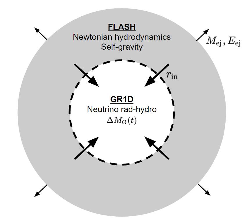
Figure 1: Schematic of our computational approach. For a given presupernova progenitor (§2.2) and dense-matter EOS, the evolution of the inner core is followed with the general-relativistic, neutrino radiation-hydrodynamics code GR1D (§2.3), focusing on the gravitational mass lost to neutrinos $\Delta M_{\rm G}(t)$ [eq. 5] at some transition radius $r_{\rm in}$. The region outside $r_{\rm in}$ is then evolved with FLASH, accounting for the mass flowing supersonically into $r_{\rm in}$ as well as the change in gravity due to $\Delta M_{\rm G}(t)$ (§2.4), and focusing on any mass ejected from the stellar surface. The majority of our models only interpolate $\Delta M_{\rm G}(t)$ from GR1D, while a smaller sample employs an analytic approximation for this function or maps the initial condition for FLASH directly from GR1D (Table 2).

Our aim is to compute the hydrodynamic response of the star to the decrease in the gravitational mass from neutrino emission after core bounce in the case where the supernova fails and a BH forms. We restrict ourselves to progenitors for which rotation is negligible, and ignore the effect of hydrodynamic instabilities that operate within the first second after bounce, which have an important role in a successful explosion (e.g., Janka et al. 2016; here we only consider failures). We therefore carry out our analysis in spherical symmetry. We also ignore any circumstellar material that the star could have ejected prior to undergoing core-collapse. This material can modify the observational signatures of shock breakout (e.g., Chevalier & Irwin 2011; Katz et al. 2012; Haynie & Piro 2020). Our focus is the total energy and mass of any ejecta arising from the change in gravitational acceleration.

In previous work (F18), we removed the inner stellar core and computed the hydrodynamic response of the star using analytic prescriptions for the evolution of the gravitational mass enclosed within this radius. This enclosed mass evolves due to material accreted through the inner radius and due to neutrino emission during the protoneutron star phase (see also Lovegrove & Woosley 2013). This modeling approach is acceptable because material that accretes through the inner boundary reaches supersonic speeds shortly after collapse, without any pressure feedback on the outer layers.

Here we replace the analytic prescriptions for the inner core evolution used in F18 with a neutrino radiation-hydrodynamic calculation (Figure 1). Due to the complexity of the latter and the limitations in thermodynamic range set by publicly available EOSs of nuclear matter, we can carry out this calculation self-consistently only until a BH forms, and within a limited volume inside the star. Nevertheless, the supersonic character of matter infall and the rapidly increasing dynamical time with stellar radius allows for a decoupling in the modeling of the inner core and the outer layers of the star with separate codes for each regime, without a significant loss in consistency.

2.2 Pre-supernova progenitors

The pre-supernova stars we explore are shown in Table 1. We adopt the same fiducial solar-metallicity progenitors as in F18: a 15 $M_{\odot}$ RSG (denoted by R15), a 25 $M_{\odot}$ BSG (B25), and a 40 $M_{\odot}$ WR (W40). These models cover three different regimes in core compactness parameter (O’Connor & Ott, 2011; Sukhbold & Woosley, 2014; Sukhbold et al., 2018)

$$\xi_{\rm 2.5}=\frac{2.5}{r(M=2.5M_{\odot})/1000\ \rm km},$$ (1)

and in envelope compactness

$$\xi_{\rm env}=\frac{(M_{\rm cc}/M_{\odot})}{(R_{\rm cc}/R_{\odot})},$$ (2)

where $M_{\rm cc}$ and $R_{\rm cc}$ are the mass and radius of the star at core-collapse. The values of $\xi_{\rm 2.5}$ and $\xi_{\rm env}$ are shown in Table 1 (see Pejcha & Thompson 2015; Ertl et al. 2016; Müller et al. 2016; Murphy & Dolence 2017 for explodability criteria other than $\xi_{\rm 2.5}$).

In addition to these baseline models, we consider two yellow supergiants (YSGs), one of 22 $M_{\odot}$ and solar metallicity (Y22), and another of 25 $M_{\odot}$ and low-metallicity (Y25); a massive 80 $M_{\odot}$ low-metallicity blue supergiant (B80); and a 50 $M_{\odot}$ solar-metallicity WR (W50). The YSGs are such than one of $\{\xi_{\rm 2.5},\xi_{\rm env}\}$ has a value similar to R15, while the other varies. W50 has a higher core-compactness than W40, and B80 has high values of both core- and envelope compactness (in F18 no mass is ejected from this model). All of these progenitors are computed with the stellar evolution code MESA version 6794 (Paxton et al., 2011, 2013, 2015, 2018). Parameters and physical choices are described in Fernández et al. (2018) (see also Fuller et al. 2015), and inlists are publicly available.

To connect with previous work, we also evolve models s20 and s40 from Woosley & Heger (2007). These progenitors have been used in BH formation simulations (e.g., O’Connor 2015; Pan et al. 2018) and in a code-comparison study of 1D core-collapse supernova simulations (O’Connor et al., 2018), providing calibration values.

Table 1: Presupernova progenitors used in this study. Columns from left to right show model name, type of star (RSG: red supergiant, YSG: yellow supergiant, BSG: blue supergiant, WR: Wolf-Rayet), zero-age main sequence mass, initial metallicity, mass at core-collapse, effective temperature at core-collapse, core compactness (eq. [1]), and envelope compactness (eq. [2]). Model S40 has the structure of a BSG but it is truncated below its photosphere.

Model	Type	M${}_{\text{zams}}$	$Z$	M${}_{\text{cc}}$	T${}_{\text{eff}}$	$\xi_{2.5}$	$\xi_{\text{env}}$
		(${M_{\odot}}$)	($Z_{\odot}$)	(${M_{\odot}}$)	($10^{3}$ K)
R15	RSG	15	1.00	11	3	0.24	0.010
B25	BSG	25	1.00	12	15	0.33	0.120
W40	WR	40	1.00	10	260	0.37	27
Y22	YSG	22	1.00	11	5	0.54	0.016
Y25	YSG	25	0.01	23	4.6	0.25	0.024
W50	WR	50	1.00	9	215	0.55	22
B80	BSG	80	0.01	55	28	0.97	0.79
S20	RSG	20	1.00	16	2.5	0.28	0.015
S40	BSG	40	1.00	15	…	0.54	1.3

2.3 Inner core evolution

The evolution of the inner stellar core from collapse until BH formation is modeled with the spherically-symmetric neutrino radiation-hydrodynamics code GR1D version 1 (O’Connor & Ott, 2010). The code solves the equations of general-relativistic hydrodynamics in spherical coordinates using the radial gauge, polar slicing metric (Romero et al., 1996). The finite-volume hydrodynamics solver employs a piecewise-parabolic reconstruction, and performs a temporal update using a second-order Runge-Kutta scheme.

During collapse, neutrino effects are modeled via a parameterization of the electron fraction with density (Liebendörfer, 2005). After bounce, neutrino cooling in this version of GR1D is modeled with a gray leakage scheme for $\nu_{\rm e}$, $\bar{\nu}_{\rm e}$ and a composite heavy lepton neutrino $\nu_{\rm x}$. The opacity has contributions from charged-current absorption on nucleons and neutral-current scattering on nucleons and nuclei. Emission accounts for charged-current reactions as well as thermal emission from electron-positron pair annihilation and plasmon decay (we did not include nucleon-nucleon bremsstrahlung). The local effective emission rate is an interpolation between the diffusive and free emission rates (Ruffert et al., 1996; Rosswog & Liebendörfer, 2003). Neutrino heating due to charge current absorption is computed from the enclosed local luminosity obtained from the leakage scheme. The local outgoing luminosity is then corrected for the neutrino energy lost to heating.

We consider three finite-temperature EOSs in our calculations: SFHo (Steiner et al., 2013) as our default (soft) case, DD2 (Hempel et al., 2012) as a stiff variant, and LS220 (Lattimer & Swesty, 1991) as another reference case. These EOSs are commonly used in the core-collapse supernova and NS merger literature (e.g., Pan et al. 2018; Vincent et al. 2020), thus providing a connection to previous work (while DD2 and SFHo are consistent with experimental constraints and unitary gas bounds on the symmetry energy and its density derivative, LS220 is not; c.f. Tews et al. 2017). We neglect light clusters when computing opacities and emissivities with the DD2 and SFHo EOSs, as these species have a sub-dominant effect on the post-bounce evolution (Yudin et al., 2019; Nagakura et al., 2019).

In most models, the computational domain is discretized with a uniform grid of $200$ cells from the origin out to $20$ km, and logarithmic spacing for larger radii, for a total grid size of $1000$ cells. In all RSG models and some YSGs and BSGs, we double the resolution in the uniform section of the grid ($r<20$ km) as these models take longer to reach BH formation and reach more compact shock radii. The maximum radius is set by a density close to the lowest value in the tabulated EOS ($2\times 10^{3}$ g cm^-3), corresponding typically to several times $10^{9}$ cm, much smaller than the radius of the star at core-collapse. The dynamical time at the outer boundary is typically $\sim 10$ s, much longer than the time to form a BH in most models, justifying our approximation of neglecting the evolution of the outer stellar layers when evolving the core with GR1D. Simulations are deemed to have formed a BH when the density increases rapidly with time to values $\sim 1-3\times 10^{15}$ g cm^-3 (near the upper limit of the EOS table), at which point the simulation stops. In only one case (model R15 with the DD2 EOS) we fail to reach BH formation within $4.37$ s of evolution and the code crashes, although based on the central value of the lapse function ($0.44$), the model is close to BH formation.

While a newer version of GR1D is available, which treats neutrinos with a multigroup moment (M1) scheme (O’Connor, 2015) and therefore provides a more accurate measure of the gravitational mass lost to neutrinos, the convergence of the transport algorithm near BH formation is more fragile than for the leakage scheme. Evolving the s40 progenitor with the LS220 EOS, we obtain post-bounce times to BH formation $\{0.561,0.556\}$ s, maximum PNS baryonic masses (at a density of $10^{12}$ g cm^-3) $\{2.448,2.372\}\,M_{\sun}$, and maximum PNS gravitational masses $\{2.309,2.246\}M_{\sun}$ with the leakage and M1 versions of GR1D, respectively. These masses and BH formation times are the same as those reported in O’Connor (2015) for the leakage version, while for the M1 version the masses are the same within $1\%$ but the BH formation time is about $4\%$ longer. These results are also consistent (within $\sim 10\%$) with the 1D results of Pan et al. (2018) for the s40 progenitor using the LS220 EOS and a different code.

2.4 Response of the star to neutrino losses

The hydrodynamic response of the outer layers of the star to the decrease in gravity due to neutrino emission is modeled in spherical symmetry with the Newtonian hydrodynamic code FLASH version 3 (Fryxell et al., 2000; Dubey et al., 2009), modified as described in Fernández (2012) and F18. The code solves the Euler equations in spherical coordinates with the dimensionally-split Piecewise Parabolic Method (PPM; Colella & Woodward 1984, Fryxell et al. 1989) and the Helmholtz EOS (Timmes & Swesty, 2000).

The computational domain spans a radial interval $[r_{\rm in},r_{\rm out}]$ that varies for different evolution modes and progenitors, as explained below. The boundary conditions are set to outflow at $r=r_{\rm in}$ and $r=r_{\rm out}$. The mass flowing out through the inner radial boundary is kept track of as a scalar baryonic mass $M_{\rm B,flash}$, such that total mass is conserved close to machine precision (F18).

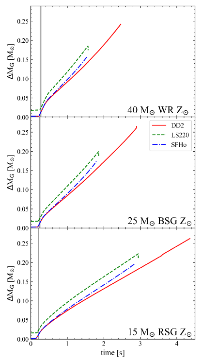
Figure 2: Evolution of the difference $\Delta M_{\rm G}$ (eq. [5]) between baryonic and gravitational masses in GR1D, evaluated at $r=2\,000$ km, as a function of time from the onset of core-collapse. Top, middle, and bottom panels correspond to our fiducial presupernova models W40, B25, and R15, respectively (Table 1). For each case, the result obtained with the DD2, SFHo, and LS220 EOS is shown, as labeled. The gray vertical band shows the range of maximum shock radius time $t_{\rm stall}$ obtained with the three EOSs ($0.204-0.220$ s for R15, $0.236-0.257$ s for B25, and $0.261-0.286$ s for W40, with the largest values corresponding to the DD2 EOS). The larger value of $\Delta M_{\rm G}$ at $t=0$ (eq. 6) for the LS220 EOS is due to an offset in the internal energy needed to connect the high- and low-density regimes of the EOS (O’Connor & Ott, 2010).

The gravitational acceleration in FLASH $\mathbf{g}_{\rm F}$ is a sum of the contribution from the baryonic mass in the computational domain and the gravitational mass $M_{\rm G,flash}$ inside $r_{\rm in}$,

$$\mathbf{g}_{\rm F}(r,t)=-\frac{G}{r^{2}}\left[M_{\rm G,flash}+4\pi\int_{r_{\rm in}}^{r}\rho(\zeta,t)\,\zeta^{2}d\zeta\right]\hat{r},$$ (3)

where $\rho$ is the mass density. Initially, the gravitational mass $M_{\rm G,flash}$ is either equal to the baryonic mass enclosed within $r=r_{\rm in}$ in the presupernova progenitor, or otherwise mapped from GR1D, depending on the mode of evolution as described below. This gravitational mass is subsequently updated from time $t_{n}$ to $t_{n+1}$ by adding the change due to the baryonic mass flowing through the inner boundary over the time step, and correcting for the instantaneous difference between baryonic and gravitational masses as computed by GR1D or from an analytic fit,

$$M_{\rm G,flash}^{(n+1)} = M^{(n)}_{\rm B,flash}+4\pi\int_{t_{n}}^{t_{n+1}}\left[r^{2}\rho\max(-v_{r},0)\right]\big{|}_{r_{\rm in}}dt$$ (4)

$$-\Delta M_{\rm G}(t_{n+1})+\Delta M_{\rm G}(t=0),$$

where

$$\Delta M_{\rm G}(t_{n})=M_{\rm B,gr1d}(t_{n})-M_{\rm G,gr1d}(t_{n}),$$ (5)

is the instantaneous difference between the baryonic and gravitational masses enclosed by $r=r_{\rm in}$ in GR1D ($M_{\rm B,gr1d}$ and $M_{\rm G,gr1d}$, respectively), and $\Delta M_{\rm G}(t=0)$ is an initial EOS-dependent offset between these two masses in GR1D

$$\Delta M_{\rm G}(t=0)\simeq 4\pi\int_{0}^{r_{\rm in}}\rho r^{2}\,dr\left[\frac{GM_{\rm G,gr1d}(r)}{c^{2}r}-\frac{e_{\rm int}}{c^{2}}\right],$$ (6)

where $e_{\rm int}$ is the specific internal energy, and we have assumed non-relativistic collapse speeds as well as $GM_{\rm G,gr1d}(r)/c^{2}\ll r$ in deriving equation (6). For the SFHo and DD2 EOSs, the term in square brackets is $\sim 10^{-3}$, whereas for LS220 it is $\sim 0.01$, given an extra offset in $e_{\rm int}$ (of order the nuclear binding energy per nucleon) needed to connect the nuclear EOS with a low-density continuation (O’Connor & Ott, 2010). Figure 2 shows the evolution of $\Delta M_{\rm G}$ at $r_{\rm in}=2\,000$ km in GR1D for our fiducial progenitors using all three EOSs considered in this study.

Since at the onset of significant neutrino emission we have $M_{\rm G,flash}\simeq M_{\rm G,gr1d}\simeq M_{\rm B,gr1d}$, the formulation in equation (4) preserves consistency in the mass evolution within FLASH, which is entirely baryonic, while also accounting for the mass-energy lost to neutrinos via $\Delta M_{\rm G}$. When a BH forms at time $t=t_{\rm bh}$, the mass difference $\Delta M_{\rm G}(t_{\rm bh})$ becomes a constant in equation (4).

The initial condition for FLASH and the evolution of the inner core ($r<r_{\rm in}$) are treated in three different ways, to assess the sensitivity of our results to the details of the inner core history (Table 2):

Table 2: Evolution modes for FLASH simulations.

	$\Delta M_{\rm G}(t)$		initial condition
	from GR1D	analytic	from GR1D
Interpolation (1)	yes	no	no
Analytic (2)	no	yes	no
Remap (3)	yes	no	yes

1. Interpolation: by default, we initialize FLASH with the pre-collapse profile, and interpolate $\Delta M_{\rm G}(t)$ at $r=r_{\rm in}$ as a function of time from GR1D. This approach provides a more realistic value for the gravitational mass lost to neutrinos relative to the models of F18, while starting from the same initial condition. Figure 2 shows the evolution the mass difference $\Delta M_{\rm G}(t)$ at $r=2\times 10^{8}$ cm for the three fiducial progenitors and EOSs used. The curves start from a very small value $\Delta M_{\rm G}(t=0)$ and increase almost linearly until BH formation. The inner radial boundary for these models is located at $r_{\rm in}=2\times 10^{8}$ cm as in F18 (approximately at the outer edge of the iron core), and $\Delta M_{\rm G}(t)$ at that radius is interpolated for use in FLASH.

2. Analytic: given the overall simplicity of the function $\Delta M_{\rm G}(t)$, we evolve a second group of models by initializing the domain in the same way as with Interpolation mode, but now we parameterize the function $\Delta M_{\rm G}(t)$ as a linear ramp that turns on and off at specified times $t_{\rm stall}$ and $t_{\rm bh}$, respectively, reaching the same maximum value as the instantaneous function $\Delta M_{\rm G}(t)$. The aim is to quantify the degree to which the details of the gravitational mass loss history (as opposed to just the final magnitude and overall timescale) influences the results. The inner boundary for these models is also located at $r_{\rm in}=2\times 10^{8}$ cm.

3. Remap: a third group of models are such that the initial condition for FLASH is mapped from GR1D, in addition to interpolating the mass difference $\Delta M_{\rm G}(t)$ at $r=r_{\rm in}$ as a function of time. Profiles of density, pressure, velocity, and composition are mapped at a time $t_{\rm stall}$ when the shock reaches its maximum amplitude, usually $\sim$ 200 ms after the onset of collapse (Figure 2). The inner radius $r_{\rm in}$ of the computational domain in FLASH is chosen such that (1) the shock radius in GR1D never exceeds it, and (2) the flow at this radius is supersonic, so that there is no hydrodynamic feedback to regions outside this transition. Figure 3 shows a snapshot of the velocity profile in a GR1D run of model W40 at the time of mapping into FLASH. For this model, $r_{\rm in}=2\times 10^{7}$ cm and the time of mapping is $\sim 270$ ms after the onset of collapse. This is not our default mode of evolution because inconsistencies between general-relativistic and Newtonian evolution are not entirely negligible at the level of precision needed to model this mass ejection mechanism.

The computational domain is discretized with a logarithmic grid using a resolution of $2\,048$ cells per decade in radius ($\Delta r/r\simeq 0.11\%$) for RSG, YSG, and BSG, models, and twice that value ($\Delta r/r\simeq 0.06\%$) for WRs. At this resolution, the pressure scale heights at the surfaces of all progenitors are resolved. We also evolve models with a lower resolution of $512$ cells per decade in radius to compare with the results of F18, which used this value in their highest resolution models.

Like in F18, following BH formation, the inner radial boundary of the simulation is moved out by a factor of $10$ at specific times, once the flow in the entire region $[r_{\rm in},10r_{\rm in}]$ has become supersonic, so that the minimum hydrodynamic time step becomes larger ($\Delta r\propto r$ in a logarithmic grid) and evolution of the shock up to the stellar surface and beyond can be followed at a smaller computational cost.

The outer radius of the computational domain in FLASH is set at $r_{\rm out}=\{2\times 10^{16},2\times 10^{15},2\times 10^{14}\}$ cm for RSG/YSG, BSG, and WR progenitors, respectively, corresponding to factors $30-1000$ times the stellar surface at core collapse. The domain outside the star is filled with a constant-density ambient medium in hydrostatic equilibrium, with the same composition as the stellar surface. The ambient densities are $\{10^{-18},10^{-16},5\times 10^{-13}\}$ g cm^-3 for RSG/YSG, BSG, and WR progenitors, respectively. These densities are low enough that the ambient mass swept up by the shock is much smaller ($\ll 1\%$) than the ejecta mass itself, with negligible slowdown. While the mass in ambient for the RSG/YSG models could in principle reach $\sim 0.1M_{\odot}$ at the maximum simulation radii, we normally stop our simulations much earlier than that point. A floor of temperature at $10^{4}$ K is adopted in all simulations, consistent with the low-temperature limit of the Helmholtz EOS in FLASH (in practice this is what sets the stopping time for RSG, YSG, and some BSG simulations). The density floor is set $100$ times lower than the ambient for RSGs, YSGs, and BSGs, and a factor of 5 lower than the ambient for WRs.

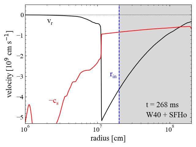
Figure 3: Velocity and sound speed as a function of radius in the core-collapse simulation of the W40 progenitor carried out with GR1D using the SFHo EOS. The time shown corresponds to that at which, when using remap evolution mode (Table 2), we map variables into FLASH for subsequent evolution. The vertical blue line indicates the position of the inner radial boundary in FLASH.

2.5 Models Evolved

All of our simulations are listed in Table 3. We adopt the SFHo EOS and interpolation of $\Delta M_{\rm G}(t)$ from GR1D (Table 2) as our default setting.

The three fiducial progenitors described in §2.2 (R15, B25, W40) are evolved using the three EOSs described in §2.3, with progenitor names appended the letters {S,L,D} when using the SFHo, LS220, or DD2 EOS, respectively, and ending in {1,2,3} in accordance to the inner core evolution modes listed in Table 2. For example, model R15S1 is the R15 progenitor evolved with the SFHo EOS in GR1D, and interpolating $\Delta M_{\rm G}(t)$ from GR1D into FLASH. We also evolve the 3 fiducial progenitors varying the evolution mode of the inner core, using the SFHo EOS. The remaining progenitors are all evolved using the SFHo EOS and interpolation of $\Delta M_{\rm G}(t)$, with the exception of the B80 progenitor, which we evolve using the SFHo and DD2 EOS.

Each progenitor is evolved at the maximum resolution listed in §2.4, while fiducial progenitors are also evolved at the lower resolution used in F18, to compare results. The maximum run time for each model is set either by the shock emerging from the star and reaching nearly constant total energy, or otherwise when the temperature in the postshock flow reaches the floor value of $10^{4}$ K, at which point non-conservation of thermal energy ensues and results become unreliable.

3 Results

Table 3: Summary of results. Columns from left to right show model name, evolution mode (I: interpolation, A: analytic, R: remap, c.f. Table 2), EOS used in GR1D, time to BH formation from the onset of core-collapse $t_{\rm bh}$, maximum gravitational mass lost to neutrinos $\Delta M_{\rm G}(t_{\rm bh})$, maximum kinetic energy of the acoustic pulse in the FLASH simulation $E^{\rm sim}_{\rm k,max}$, mass ejected in the FLASH run $M_{\rm ej}$, total energy of ejecta in FLASH run $E_{\rm ej}$, and recombination energy $E_{\rm rec}$ (eq. 9) for stars with extended hydrogen envelopes. Results are reported for FLASH runs at their maximum resolution, see §3.4 for results at lower resolution. Model W40S1.7 has its inner radial boundary at $r_{\rm in}=2\times 10^{7}$ cm, instead of the default $r_{\rm in}=2\times 10^{8}$ cm for interpolation mode.

Model	Mode	EOS	$t_{\rm bh}$ (s)	$\Delta M_{\text{G}}$ ($M_{\odot}$)	$E^{\rm sim}_{\rm{k,max}}$ ($10^{47}$ erg)	$M_{\text{ej}}$ (${M_{\odot}}$)	$E_{\text{ej}}$ ($10^{47}$ erg)	$E_{\rm rec}$ ($10^{47}$ erg)
R15S1	I	SFHo	2.836	0.196	2.15	2.19	-0.119	0.398
R15S2	A				2.06	2.16	-0.154	0.388
R15S3	R				0.57	0.99	-0.268	0.179
R15L1	I	LS220	2.947	0.222	2.42	2.42	-0.103	0.440
R15D1		DD2	$>$4.359	$>$0.262	3.59	3.37	0.489	0.612
S20S1		SFHo	2.188	0.173	0.69	0.70	-0.320	0.128
						$M_{\text{ej}}$ ($10^{-2}$ ${M_{\odot}}$)
B25S1	I	SFHo	1.791	0.173	2.27	2.80	0.399
B25S2	A				2.27	2.82	0.404
B25S3	R				0.14	0.45	0.012
B25L1	I	LS220	1.864	0.198	2.55	3.18	0.593
B25D1		DD2	2.895	0.261	5.40	5.45	1.76
Y22S1		SFHo	0.931	0.139	0.55	5.39	-0.013	0.010
Y25S1			2.542	0.175	3.18	15.5	-0.082	0.028
						$M_{\text{ej}}$ ($10^{-4}$ ${M_{\odot}}$)
W40S1	I	SFHo	1.535	0.157	1.40	1.44	0.067
W40S2	A				1.36	1.36	0.063
W40S3	R				0.06	0.01	$<$0.001
W40L1	I	LS220	1.570	0.184	1.52	1.63	0.077
W40D1		DD2	2.466	0.242	3.92	6.30	0.326
W40S1.7		SFHo	1.535	0.157	1.68	1.91	0.090
W50S1			0.895	0.126	0.53	0.54	0.019
B80S1			0.624	0.074	0.09	0.76	-0.001
B80D1		DD2	0.706	0.115	0.21	2.13	-0.002
S40S1		SFHo	0.943	0.128	0.13	1.07	$<$0.001

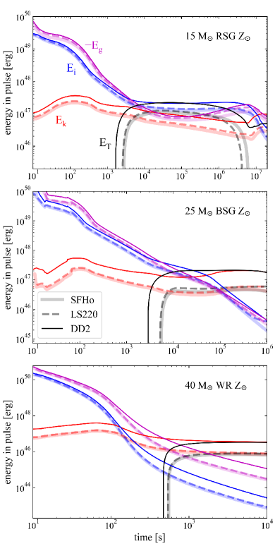
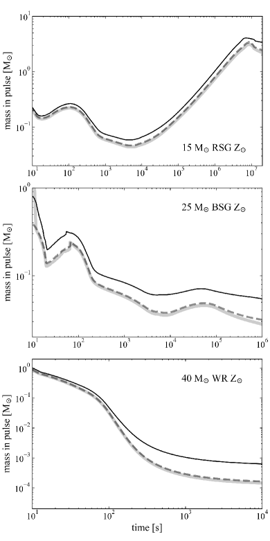
Figure 4: Left: Evolution of the energy components in the acoustic pulse generated by neutrino-induced gravitational mass decrease for our three fiducial progenitors: R15 (top), B25 (middle), and W40 (bottom). Each panel shows the kinetic (red), internal (blue), gravitational (purple), and total energy (black) for models that interpolate $\Delta M_{\rm G}(t)$ from GR1D and vary the EOS: DD2 (thin solid), SFHo (thick semitransparent), and LS220 (dashed). Only positive total energies are shown. Right: Evolution of the mass contained by the pulse. Curves correspond to the same models as in the left panel.

3.1 Overview of evolution for different progenitors

The inner core evolution in all of our models is qualitatively the same. After core-collapse and bounce, the shock stalls and then gradually recedes on a timescale of $\sim$ 1 s, as expected for non-rotating iron core progenitors evolved in spherical symmetry (Liebendörfer et al., 2001; Rampp & Janka, 2002; Thompson et al., 2003; Sumiyoshi et al., 2005). With the exception of model R15D1, a BH forms within $3$ s after bounce. At that time, the difference between baryonic and gravitational masses $\Delta M_{\rm G}$ stops increasing, as shown in Figure 2.

At a radius $\sim 10^{9}$ cm, where the local free-fall time $t_{\rm ff}$ is comparable to the time to change the gravitational mass via neutrino cooling ($\sim t_{\rm bh}$), an acoustic pulse forms which moves outward with a Mach number of order unity (F18; Coughlin et al. 2018a). The subsequent evolution of this sonic pulse and its effect on the stellar envelope depends on the type of stellar progenitor. Table 3 summarizes the results of our hydrodynamic simulations.

For models in which we initialize the domain in FLASH by remapping fluid quantities from GR1D at $t=t_{\rm stall}$ (evolution mode 3 in Table 2), there are discrepancies at the $\lesssim 10\%$ in the fluid quantities (slightly lower density, lower internal energy, differing infall velocity) within the outermost mapping radius ($\sim 10^{9}$ cm) relative to the presupernova model. This results in the remapped models undergoing a slighly faster collapse than corresponding models that only make use of $\Delta M_{\rm G}(t)$ to modify gravity (evolution modes 1 and 2), which yields either a reduced kinetic energy of the shock and lower amount of mass ejected (models R15S3 and B25S3) or no mass ejected at all (model W40S3). Resolving this discrepancy requires a self-consistent treatment of the entire star using a general-relativistic framework, which is beyond the scope of our study. In the rest of the paper we limit the discussion to models that only interpolate $\Delta M_{\rm G}(t)$ from GR1D or otherwise approximate it analytically.

Figure 4 shows the evolution of the energy in the sound pulse as it travels outward through the envelope and becomes a running shock, for our three fiducial progenitors. Following F18, we define the pulse shell as the region limited by the forward edge of the pulse/shock on its front, and by the stagnation point on its rear, which separates expanding from accreting flow. Figure 4 also shows that the mass in this pulse changes with time, as it sweeps up material on its front and loses it to fallback accretion from its rear. In all cases, the kinetic energy in the pulse is initially a small fraction of the gravitational and internal energies in the shell. As the pulse propagates out, the kinetic energy eventually becomes comparable and/or exceeds the (more rapidly decreasing) thermal and gravitational energies as it emerges from the stellar surface. The final net energy of the outgoing shock is comparable to its initial kinetic energy.

The propagation of weak shocks in gravitationally bound stellar envelopes does not conserve energy (Coughlin et al., 2018b). Depending on the radial dependence of the stellar density profile and on the initial strength of the pulse, the shock can accelerate or decelerate, yielding behavior that ranges from a strong shock as it reaches the stellar surface to fizzling as a rarefaction wave that ejects a negligible amount of mass (Coughlin et al. 2019; Ro et al. 2019; see also Linial et al. 2020).

The energy of the acoustic pulse can be understood to order of magnitude from the impulse $\Delta v_{\rm pulse}$ imparted to a mass shell by the change in gravity over a free-fall time $t_{\rm ff}$, $\Delta v_{\rm pulse}(r)=(G\Delta M_{\rm G}/r^{2})\,t_{\rm ff}$ (Coughlin et al. 2018a, F18). The kinetic energy in the pulse is

$$\Delta E_{\rm pulse}\simeq\frac{1}{2}M_{\rm pulse}\Delta v_{\rm pulse}^{2},$$ (7)

with $M_{\rm pulse}\simeq 4\pi r^{2}H_{\rm p}$, and $H_{\rm p}$ being the pressure scale height. In terms of stellar quantities, we can write the maximum kinetic energy that a stellar shell can have as (F18)

$$E_{\rm k,\,max}\simeq 2.5\times 10^{47}\left(\frac{\alpha}{0.4}\right)\left(\frac{H_{\rm p}/r}{0.4}\right)\left(\frac{\Delta M_{\rm G}}{0.15M_{\odot}}\right)^{2}$$ (8)

$$\qquad\qquad\times\left(\frac{2\times 10^{9}\,\textrm{cm}}{r}\right)\,\textrm{erg}~{},$$

where we have evaluated equation (7) at the location where energy extraction is maximal (point of acoustic pulse formation), and where $\alpha=d\ln M(r)/d\ln r$. The maximum kinetic energies obtained in the simulations (Figure 4, also shown in Table 3 as $E^{\rm sim}_{\rm k,max}$) are broadly consistent with equation (8) given the characteristic gravitational mass changes $\Delta M_{\rm G}(t_{\rm bh})$ shown in Table 3.

The mass ejected via this mechanism is set, to order of magnitude, by the exterior mass coordinate in the star at which the gravitational binding energy is comparable to the shock energy. RSGs, with weakly bound hydrogen envelopes, can eject several solar masses of slowly-moving material (Lovegrove & Woosley, 2013), whereas BSGs and WR stars eject much smaller masses at higher speeds (F18).

Figure 5 shows the ejecta mass and energies as a function of core compactness (eq. 1) and envelope compactness (eq. 2), for all of our simulations that interpolate $\Delta M_{\rm G}(t)$ from GR1D runs that use the SFHo EOS. The inverse relation between ejected mass and envelope compactness is evident: given shock energies of characteristic magnitude of $\sim 10^{47}$ erg, the mass ejected is inversely proportional to the surface gravity of the star. The inverse dependence of the ejecta energy with core compactness can be understood from the monotonic decrease in $\Delta M_{\rm G}(t_{\rm bh})$ with core compactness (Figure 6). Higher compactness is associated with a shorter time to BH formation (O’Connor & Ott, 2011; da Silva Schneider et al., 2020), which results in less gravitational mass lost to neutrinos. While the ejecta energy is weakly correlated with envelope compactness, the energy per unit mass (and hence velocity) of the ejecta is strongly dependent on the envelope compactness (Figure 6): stars that can unbind matter from their surfaces do so at speeds that scale with the escape velocity at that location ($v_{\rm esc}\propto\xi_{\rm env}^{1/2}$).

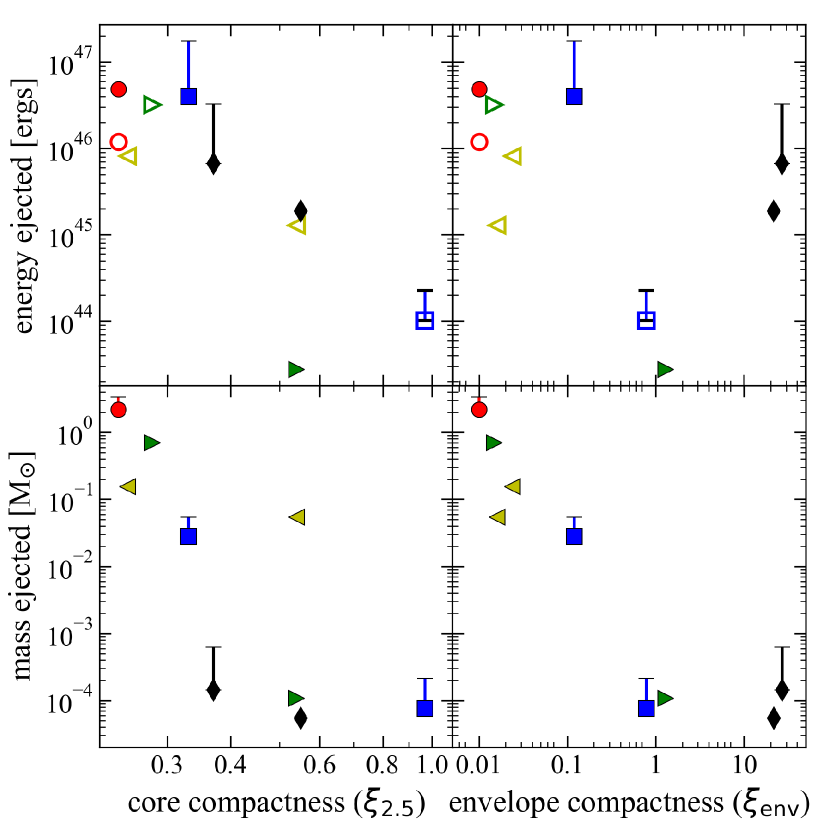
Figure 5: Ejecta energy (top) and mass (bottom) as a function of core compactness $\xi_{2.5}$ (left; eq. 1) and envelope compactness $\xi_{\rm env}$ (right; eq. 2) for all models that interpolate $\Delta M_{\rm G}(t)$ from GR1D using the SFHo EOS. The error bars indicate the change introduced, for our 3 fiducial progenitors (R15, B25, W40), by evolving the inner core with the DD2 EOS instead. Colored markers correspond to their respective progenitors: red circles for RSGs, blue squares for BSGs, black diamonds for WRs, yellow left triangles for YSGs, green right triangles for S20 and S40 models. Open and full symbols in the top row denote bound and unbound ejecta, respectively, with the exception of the R15 models, for which we have plotted both R15S1 (open circle, bound) and R15D1 (full circle, unbound).

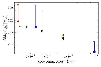
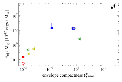
Figure 6: Left: Maximum gravitational mass lost to neutrino emission $\Delta M_{\rm G}(t_{\rm bh})$ as a function of core compactness $\xi_{2.5}$. Right: Ejecta energy per unit mass as a function of envelope compactness $\xi_{\rm env}$. Symbols and error bars have the same meaning as in Figure 5, with the extra high-compactness BSG on the left panel representing model B80S1, which does not eject mass. An upper limit is used for $\Delta M_{\rm G}(t_{\rm bh})$ from model R15D1 since it did not collapse to a BH in GR1D within $4.2$ s of evolution.

To illustrate these trends with specific cases, we can compare models R15S1 and Y22S1, which have similar envelope compactness (0.010 and 0.016 respectively), but the YSG has more than double the core compactness of the RSG (0.54 versus 0.24, respectively). Model R15S1 ejects about 2.2 ${M_{\odot}}$, a factor of 40 more than the YSG ejecta (5.39$\times 10^{-2}$${M_{\odot}}$), which follows from the larger value of $\Delta M_{\rm G}(t_{\rm bh})$ for the RSG. In both cases, the ejecta is bound (see §3.2 for a discussion of hydrogen recombination energy). Likewise, models R15S1 and Y25S1 have similar core compactness (0.24 and 0.25, respectively), but the YSG’s envelope compactness is more than double that of the RSG (0.010 and 0.024, respectively). The Y25 model ejects $0.155$${M_{\odot}}$, which is approximately 14 times less compared to the $\sim$ 2.2${M_{\odot}}$ from the RSG. In both cases the ejecta is bound, with the energy per unit mass being larger in the YSG. Model S20S1 has higher core and envelope compactness than model R15S1, and also ejects bound mass.

Model B80S1 has a higher core (0.97) and envelope compactness (0.79) than model B25S1 (0.33 and 0.12 respectively). While B25S1 ejects 2.8$\times 10^{-2}$ ${M_{\odot}}$with energy $4\times 10^{46}$ erg by the end of the simulation, model B80S1 generates a shell with mass $\sim 8\times 10^{-5}$ ${M_{\odot}}$  that is bound ($E_{\rm ej}$ $\sim$ $-10^{44}$ erg) by the time it approaches the stellar surface and reaches the floor of temperature (after which time the internal energy starts rising and the subsequent evolution is unreliable). This $80$ ${M_{\odot}}$  progenitor also fails when using parameterized neutrino mass loss in F18. Model S40S1, in contrast, is a BSG with similar envelope compactness as B80S1 but smaller core compactness (0.54), ejecting marginally bound mass in amounts comparable to the WR models, which have much higher envelope compactnesses.

Model W50S1 has a higher core compactness than model W40S1 (0.55 and 0.37 respectively), but a lower envelope compactness (22 and 27, respectively). Model W50S1 ejects less mass and with lower energy (5.4$\times 10^{-5}$ ${M_{\odot}}$  and 1.9$\times 10^{45}$ erg) than W40S1 (1.4$\times 10^{-4}$ ${M_{\odot}}$and 6.7$\times 10^{45}$ erg). While the energy per unit mass is comparable, it is higher in the progenitor with higher envelope compactness (W40S1).

A systematic uncertainty of $\sim 10\%$ in our results using the default evolution mode arises from our choice of $r_{\rm in}=2\times 10^{8}$ cm. Model W40S1.7 is identical to W40S1 except for the position of the inner radial boundary set at $r_{\rm in}=2\times 10^{7}$ cm. The resulting ejecta mass and energy are about $30\%$ higher in the model with the smaller inner radial boundary (see also F18 for further tests on the sensitivity of the choice of boundary position).

3.2 EOS Dependence

Table 3 shows that for the same stellar model and spatial resolution, using the stiffer DD2 EOS to evolve the inner core results in more mass ejected and with higher specific energy, by a factor of several, relative to using the softer SFHo or LS220 EOS. Equation (8) shows that the maximum kinetic energy of the shock is proportional to the square of the gravitational mass lost to neutrinos $\Delta M_{\rm G}$. All models evolved with the DD2 EOS achieve higher values of $\Delta M_{\rm G}(t_{\rm bh})$ than their equivalent models evolved with the SFHo EOS by a factor of up to two. Results obtained with the SFHo and LS220 EOSs are usually very similar to each other and often overlap.

The origin of this trend with EOS stiffness is illustrated in Figure 2: the stiffer DD2 EOS yields a longer time to BH formation and therefore results in more gravitational mass lost to neutrino emission than in the models that use the SFHo EOS. While there are some differences in the growth rate of $\Delta M_{\rm G}$, associated with the differing neutrino luminosities, which in turn are most sensitive to the effective nucleon masses in the EOS (Schneider et al., 2019), these luminosity differences are sub-dominant compared to those arising from the time interval during which the PNS emits neutrinos, which is set primarily by the accretion rate and the maximum mass at finite entropy ($M_{\rm tov}$) that the EOS can support, which depends on both cold and thermal pressure components (Hempel et al., 2012; da Silva Schneider et al., 2020). The same trend of increasing ejecta mass and energy with increasing $M_{\rm tov}$ was found by Lovegrove & Woosley (2013) using a parameterized evolution of the inner core.

Figure 5 shows the spread in ejected masses due to the EOS (represented as error bars) for our three fiducial progenitors. Aside from the magnitude of the gravitational mass lost and a minor change in the location of the acoustic pulse formation (radius at which $t_{\rm bh}\simeq t_{\rm ff}$), the evolution of the shock as it propagates into the envelope is qualitatively the same for all EOSs, as shown in Figure 4

A key quantitative difference introduced by the EOS is that when using SFHo or LS220, none of the RSG progenitors eject unbound mass (Table 3). The equation of state used in FLASH assumes fully ionized nuclei, but it is known that hydrogen recombination can dominate the energetics upon subsequent expansion of the shock in failed supernovae from RSGs (Lovegrove & Woosley, 2013). To estimate the importance of this missing effect, we compute the recombination energy $E_{\rm rec}$ that can be liberated if all the hydrogen contained in the ejecta recombines to the ground state,

$$E_{\rm rec} = \frac{M_{\rm H}}{m_{\rm p}}\chi_{\rm H}$$ (9)

$$M_{\rm H} = \int_{0}^{M_{\rm ej}}X(M)dM,$$ (10)

with $X$ the mass fraction of hydrogen in the ejecta, $m_{\rm p}$ the proton mass, and $\chi_{\rm H}=13.6$ eV. The resulting recombination energies for RSGs and YSGs are shown in Table 3. With the exception of model s20 and the model that maps initial profiles from GR1D (R15S3), the ejecta for all other RSG progenitors should be unbound after including this contribution. Regarding YSGs, model Y22S1 can potentially unbind its ejecta marginally when including hydrogen recombination (e.g., with a more precise calculation than our rough estimate), while for model Y25S1 recombination energy falls short by a factor 3 and unbinding is unlikely.

Table 4: Comparison of the ejecta masses and energies obtained in F18 (high-resolution “e_HR” models, using parametric inner core evolution) and in this work (interpolating $\Delta M_{\rm G}(t)$ from GR1D using either the SFHo [S1] or DD2 [D1] EOS and at the same resolution as F18; c.f. Table 5), for our three fiducial progenitors (Table 1).

Progenitor	$M_{\rm ej}(M_{\odot})$		$E_{\rm ej}(10^{47}$ erg)
	[S1,D1]	F18	[S1,D1]	F18
R15	[2.2, 3.4]	4.2	[-0.1, 0.5]	1.9
B25	[0.03, 0.05]	0.05	[0.5, 1.8]	1.6
W40	[1, 6]$\times 10^{-4}$	$5\times 10^{-4}$	[0.06,0.31]	0.25

The massive BSG progenitor B80 fails with both the SFHo and DD2 EOSs. While the latter yields a larger shock kinetic energy by a factor $\sim 2$, the qualitative result does not change: as the shock approaches the stellar surface, it reaches the floor of temperature and the internal energy begins rising. Prior to that, the mass in the shell is $\lesssim 10^{-4}$ $M_{\odot}$ and the outward-moving material is gravitationally bound with $E_{\rm ej}\simeq-10^{44}$ erg. Further study of these failing models will require a low-temperature EOS consistent with that used to evolve the presupernova model.

Comparing to the results of F18, which were obtained using an analytic model for the inner core evolution and therefore of $\Delta M_{\rm G}(t)$, we find that their results are in broad agreement with our models that use the DD2 EOS. In contrast, results obtained with the softer SFHo EOSs have energies lower by a factor of several compared to F18. A side-by-side comparison of results for the same fiducial progenitors and at the same spatial resolution is shown in Table 4. The relation between the two sets of results follows from the fact that F18 assumed $M_{\rm tov}=2.5$ $M_{\odot}$ as an input to their parametric neutrino scheme. The maximum NS mass at an entropy of $4k_{\rm B}$ per baryon correlates well with $t_{\rm bh}$ when comparing among different EOSs (Hempel et al., 2012). The choice of F18 is much closer to the finite-entropy $M_{\rm tov}$ for the DD2 EOS ($2.57$ ${M_{\odot}}$ at $4k_{\rm B}$ per baryon; M. Hempel, private communication) than for the SFHo EOS ($2.3$ ${M_{\odot}}$ at $4k_{\rm B}$ per baryon, Steiner et al. 2013).

3.3 Simplified inner core evolution: linear ramp for $\Delta M_{\rm G}$

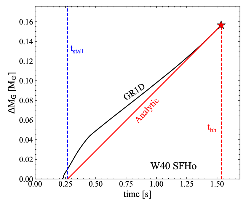
Figure 7: Evolution of $\Delta M_{\rm G}$ as a function of time since core-collapse for the W40 progenitor. The result from GR1D using the SFHo EOS is shown in black, while our linear ramp parameterization is shown in red, with the star denoting the time of BH formation. The vertical dashed blue line shows the time $t_{\rm stall}$ at which the shock stalls, which we use to start the ramp function (same time as in Figure 3). The vertical dashed red line shows the time of BH formation t_bh.

To assess the sensitivity of mass ejection to the detailed history of neutrino emission by the protoneutron star before BH formation, we explore a set of models in which we parameterize $\Delta M_{\rm G}(t)$ as a linear ramp in time (Figure 7). The input parameters are the maximum value of $\Delta M_{\rm G}$, the time of BH formation $t_{\rm bh}$, and a starting time, which we choose to be that when the shock radius reaches its maximum value ($t_{\rm stall}$, same as that used when remapping the domain from GR1D). These parameters are generally reported in (or otherwise are straightforward to obtain from) published studies of BH formation in failed SNe.

Figure 8 compares the evolution of the energy, mass, and velocities of the outgoing shell for models W40S1 and W40S2, with the former interpolating $\Delta M_{\rm G}(t)$ from GR1D and the latter using the analytic ramp prescription. The shock properties are very close to one another in both models, with a relative difference of $6\%$ in energy and in mass by the end of the simulation. A smaller relative difference in final energy and mass (few percent) is found for the corresponding BSG models (B25S1-B25S2), while for the RSG the mass ejected is nearly the same whereas the negative ejecta energy differs by 30% (Table 3).

The low sensitivity to the detailed neutrino history can be understood from the fact that variations in neutrino emission (as inferred from Figure 2) occur on timescales much shorter than $t_{\rm bh}$. Mass shells for which the local dynamical time $t_{\rm dyn}$ is comparable to this neutrino variability timescale are accreted into the BH before there is sufficient time to affect the emergence of the sound pulse at a location such that $t_{\rm dyn}\sim t_{\rm bh}$. Marginally bound shocks (from RSGs) are more sensitive to small changes in neutrino emission history than those from progenitors that eject mass more robustly.

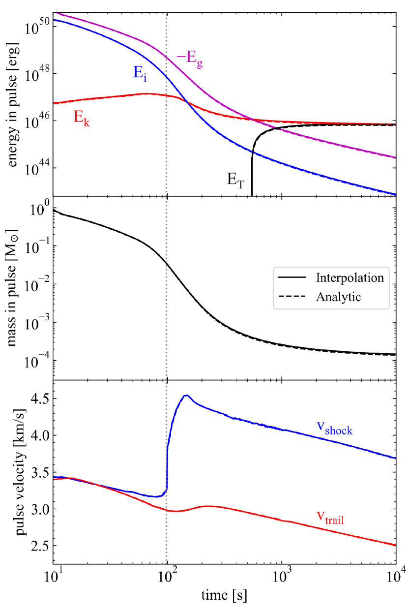
Figure 8: Comparison between models W40S1 and W40S2, which interpolate $\Delta M_{\rm G}(t)$ from GR1D or use an analytic ramp model (Figure 7), respectively. Top, middle, and bottom panels show the evolution of the energies, mass, and velocity of the sound pulse, as labeled ($v_{\rm shock}$ and $v_{\rm trail}$ are the velocities of the forward and rear end of the shell, respectively). The vertical dotted line indicates the time at which the shock emerges from the stellar surface.

3.4 Effect of spatial resolution

Table 5: Resolution dependence of key quantities for selected models. Columns from left to right show model name, EOS used in GR1D, spatial resolution in the FLASH run ($\Delta r/r=\{4.5,1.1,0.6\}\times 10^{-3}$ corresponds to $\{512,2048,4096\}$ cells per decade in radius in a logarithmic grid), mass ejected in the FLASH run $M_{\rm ej}$, total energy of ejecta in the FLASH run $E_{\rm ej}$, shock breakout velocity measured in the FLASH simulation, and analytic breakout velocity (eq. [11]).

Model	EOS	$\Delta r/r$	$M_{\text{ej}}$	$E_{\text{ej}}$	$v^{\rm num}_{\rm bo}$	$v^{\rm WK}_{\rm bo}$
		($10^{-3}$)	$({M_{\odot}})$	($10^{47}$ erg)	(km s-1)	(km s-1)
R15S1	SFHo	4.5	2.20	-0.130	60	…
R15S1		1.1	2.19	-0.119	60	…
R15D1	DD2	4.5	3.38	0.498	80	30
R15D1		1.1	3.37	0.489	80	30
			$M_{\text{ej}}$
			($10^{-2}$ ${M_{\odot}}$)
B25S1	SFHo	4.5	2.90	0.491	900	600
B25S1		1.1	2.80	0.399	1,000	500
B25D1	DD2	4.5	5.46	1.77	1,300	900
B25D1		1.1	5.45	1.76	1,300	900
			$M_{\text{ej}}$
			($10^{-4}$ ${M_{\odot}}$)
W40S1	SFHo	4.5	1.32	0.059	9,000	9,000
W40S1		0.6	1.44	0.067	17,000	10,000
W40D1	DD2	4.5	6.15	0.308	10,000	13,000
W40D1		0.6	6.30	0.326	20,000	13,000

Table 3 reports the mass ejected and final shock energy for selected models at two spatial resolutions: the same as in F18 ($\Delta r/r=4.5\times 10^{-3}$) for comparison, and at 4-8 times finer grid spacing per decade in radius ($\Delta r/r=0.6-1.1\times 10^{-3}$). The highest resolution is used to resolve the surface pressure scale height of the W40 model with $\sim 3$ cells ($H_{\rm p}/R_{\rm cc}\simeq 1.5\times 10^{-3}$). For RSGs and BSGs, the surface pressure scale height is resolved with $\{2-10,4-20\}$ cells in our low-high resolution models, respectively.

The ejecta masses and energies are essentially converged with resolution for the RSG and BSG models that use the DD2 EOS (R15D1 and B25D1). Their SFHo counterparts (R15S1 and B25S1), with weaker explosions, are somewhat sensitive to resolution, with changes of a few percent in their ejected mass and $10-20\%$ in ejecta energies when increasing the resolution by a factor 4. For the WR progenitor, on the other hand, resolving the surface pressure scale height even with a few cells results in an increase of $10\%$ in ejecta mass and energy for model W40S1, with a $2-5\%$ change in the more energetic model W40D1. We expect further increases in resolution to behave in the same way as for RSG and BSG models. As discussed in §3.1, an additional $\sim 10\%$ uncertainty in ejecta mass and energy arises from the position of the inner radial boundary.

As an additional diagnostic of our simulations, we examine the velocity at shock breakout, and compare with analytic formulae (as reviewed in Waxman & Katz 2017). The latter predict a shock breakout velocity

$$v_{\rm bo}^{\rm WK}\simeq v_{*}\times\begin{dcases}13\,M_{\rm ej,10}^{0.16}\,v^{0.16}_{*,8.5}\,R^{-0.32}_{\rm cc,12}&\qquad(\textrm{BSG, WR})\\ \vskip 3.0pt plus 1.0pt minus 1.0pt\cr 4.5\,M_{\rm ej,10}^{0.13}\,v^{0.13}_{*,8.5}\,R^{-0.26}_{\rm cc,12}&\qquad(\textrm{RSG}),\end{dcases}$$ (11)

where $v_{*}=\sqrt{E_{\rm ej}/M_{\rm ej}}$, $M_{\rm ej,10}=M/(10{M_{\odot}})$, $v_{*,8.5}=v_{*}/(10^{8.5}\textrm{\,cm\,s}^{-1})$, and $R_{\rm cc,12}=R_{\rm cc}/(10^{12}\textrm{\,cm})$, and where we have ignored the dependence on opacity and detailed stellar density profile dependence. The corresponding values of $v_{\rm bo}^{\rm WK}$ are shown in Table 5 for selected models.

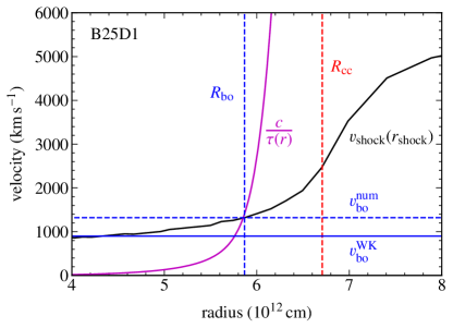
Figure 9: Forward shock velocity $v_{\rm shock}$ as a function of forward shock radius $r_{\rm shock}$ in model B25D1 at high resolution. The numerical shock breakout velocity $v_{\rm bo}^{\rm num}$ is obtained by searching for the position at which $v_{\rm shock}=c/\tau(r)$, where $\tau(r)$ is the optical depth in the presupernova star. For reference, we also show the analytic value $v_{\rm bo}^{\rm WK}$ from equation (11). The numerical shock velocity is not smoothed for this model.

The shock breakout velocity is measured from the FLASH simulations as follows. We use the position of the forward shock $r_{\rm shock}$ as a function of time to calculate the forward shock velocity $v_{\rm shock}$ using time-centered finite difference. When the resulting velocity curve is too noisiy, we smooth this function using a Savitsky-Golay filter to suppress fluctuations. We then obtain the shock breakout velocity by an iterative process: we start with the shock velocity at the stellar surface, and compute the shock breakout optical depth $\tau_{\rm bo}=c/v_{\rm shock}$, which is then used to obtain the shock breakout radius $R_{\rm bo}$ using the optical depth profile in the presupernova progenitor. The shock velocity at the newly obtained position $r=R_{\rm bo}$ is then used to compute a new optical depth, which then yields another value for $R_{\rm bo}$. This process converges after a few iterations.

Table 5 shows the numerical shock breakout velocities for selected models. Agreement with analytical values is good to within a factor of $2$. Figure 9 shows an example of the forward shock velocity profile and its relation to the analytic value for model B25D1.

Given that our simulations resolve the surface pressure scale height in all models, we revisit the prediction of Coughlin et al. (2018a) regarding the outward acceleration of the photosphere ahead of the main shock. A photospheric shock is possible given that the entire envelope experiences a nearly instantaneous change in the acceleration of gravity, and regions near the surface of the star have a rapidly decreasing sound speed with radius. Figure 10 shows radial profiles of velocity at a time when the main shock is about to reach the original pre-collapse surface at $r=R_{\rm cc}$.

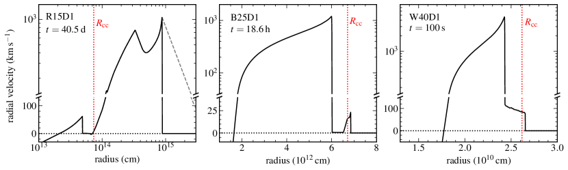
Figure 10: Radial velocity profile of stellar matter at a time just before the main shock reaches the pre-collapse stellar surface (red vertical line labeled $R_{\rm cc}$), for selected models at their highest resolutions. The gas near the photosphere acquires positive velocity even before the arrival of the shock, with noticeable ‘surface’ shocks in the RSG and BSG models. The dashed grey line shows the velocity of ambient material in model R15D1 (the main shock has a smaller velocity but carries more mass than the surface shock).

The RSG model is such that outward acceleration of matter near the photosphere is very efficient, launching a series of surface shocks that reach $\sim 10\,R_{\rm cc}$ by the time the main shock approaches the stellar surface. These surface shocks contain very little mass, and include ambient material. Part of this dynamics is likely to arise from the temperature being near the floor value of the EOS ($10^{4}$ K), which is higher than the actual surface temperature of the RSG and therefore implies inconsitent thermodynamics (fully ionized ions assumed in FLASH) relative to the EOS used to construct the presupernova model.

A cleaner surface shock is visible in the BSG model, which displays a quiescent ambient ahead of it. The magnitude of this surface shock is smaller by a factor of almost $\sim 100$ compared to the main shock, and it does not lead to a significant expansion of the stellar surface ahead of the arrival of the main shock. For the WR model, the entire region inside the photosphere moves outward at $\sim 100$ km s^-1 and, while no independent shock is visible before the arrival of the much faster main shock, this photospheric expansion is significantly faster than in the RSG and BSG models, as predicted by Coughlin et al. (2018a). Like in the BSG model, however, the expansion of the star is minimal before the arrival of the main shock.

3.5 Implications for electromagnetic counterparts

Table 6: Estimates for the bolometric shock breakout and plateau emission for our fiducial progenitors, which interpolate $\Delta M_{\rm G}(t)$ from GR1D and use the DD2 or SFHo EOS. Columns from left to right show: model name, shock breakout luminosity, breakout time (maximum between diffusion and light-crossing times), shock velocity at breakout $v_{\rm bo}$, effective temperature at breakout $T_{\rm bo}$, plateau luminosity, plateau duration, and final shock velocity $v_{\rm exp}=\sqrt{2E_{\rm ej}/M_{\rm ej}}$. Model R15S1 ejects bound material so no plateau properties are computed, and the breakout velocity is obtained from the simulation (Table 5); for all other models the breakout velocity is computed using equation (11). For reference, the pre-supernova luminosities are $\{1.3,3.8,5.7\}\times 10^{5}L_{\odot}$ for models R15, B25, and W40, respectively.

Model	$L_{\rm bo}$	$t_{\rm bo}$	$v_{\rm bo}$	$T_{\rm bo}$	$L_{\rm pl}$	$t_{\rm pl}$	$v_{\rm exp}$
	($10^{6}$ ${L_{\odot}}$)		(km s-1)	($10^{4}$ K)	($10^{5}$ ${L_{\odot}}$)	(d)	(km s-1)
R15S1	$0.7$	$4$ d	$60$*	$0.5$	…	…	…
R15D1	$2$	$8$ d	$40$	$0.6$	$2$	$400$	$40$
B25S1	$50$	$6$ h	$500$	$5$	$9$	$20$	$400$
B25D1	$300$	$3$ h	$900$	$8$	$20$	$20$	$600$
W40S1	$400$	$1$ s	$9,600$	$140$	$0.3$	$1$	$2,000$
W40D1	$600$	$1$ s	$13,000$	$150$	$0.6$	$2$	$2,000$

Non-rotating failed supernovae are expected to generate electromagnetic emission in the form of shock breakout (Piro, 2013; Lovegrove et al., 2017) and plateau emission (Lovegrove & Woosley, 2013). The predicted plateau properties for a RSG progenitor are consistent with those of the failed supernova candidate N6946-BH1 (Gerke et al., 2015; Adams et al., 2017; Basinger et al., 2020). A wider range in emission properties is expected when accounting for WRs and BSGs (F18).

Following F18, we estimate bolometric shock breakout properties in our models using a combination of analytic formulate and quantities measured from the FLASH simulations. The shock breakout luminosity is estimated as (Piro, 2013)

$$L_{\rm bo}\simeq\frac{E_{\rm rad}}{\max(t_{\rm lc},t_{\rm diff})},$$ (12)

where $t_{\rm lc}=R_{\rm cc}/c$ is the light-crossing time over the stellar radius and $t_{\rm diff}=(R_{\rm cc}-R_{\rm bo})/v_{\rm bo}$ is the radiation diffusion (and shock crossing) time, with $R_{\rm bo}$ the stellar radius at which the optical depth is $c/v_{\rm bo}$. The radiation energy $E_{\rm rad}$ is obtained for WRs using the formulae in Waxman & Katz (2017), while for BSGs and RSGs it is measured directly from the simulation ($E_{\rm rad}=\int aT^{4}dV$ over the volume between $R_{\rm bo}$ and $R_{\rm cc}$ at the time when $r_{\rm shock}=R_{\rm cc}$). The shock breakout velocity is set to the analytic value in equation (11) except for model R15S1, which has $E_{\rm ej}<0$, in which case we use the value obtained from the simulation (Table 5). The temperature of the breakout emission is estimated using the luminosity and stellar radius, $L_{\rm bo}=4\pi R_{\rm cc}^{2}\,\sigma T_{\rm bo}^{4}$.

Table 6 shows the shock breakout emission estimates for our fiducial models employing the DD2 or SFHo EOSs. For reference, the pre-supernova luminosities are $\{1.3,3.8,5.7\}\times 10^{5}L_{\odot}$ for models R15, B25, and W40, respectively. In all cases, the shock breakout luminosity exceeds the presupernova luminosity, with characteristic values $\sim 10^{39}$, $10^{41}$, and $10^{42}$ erg s^-1 for RSG, BSG, and WR, respectively. The timescales range from days, hours, and seconds, and the emission is dominated by optical, UV, and X-rays, for RSGs, BSGs, and WRs, respectively. These estimates ignore the effects of an intervening wind (e.g., Chevalier & Irwin 2011; Katz et al. 2012; Haynie & Piro 2020), hence they are likely very rough, particularly for WRs. The EOS introduces a variation of a factor of a few in luminosity and timescale, while the uncertainty in breakout velocity (Table 5) adds another factor of $2$ uncertainty. Overall, resuls are qualitatively the same as those from F18, as expected from Table 4

Plateau emission is estimated using the formulae of Kleiser & Kasen (2014)

$$L_{\rm pl} = 1.2\times 10^{42}E_{\rm ej,51}^{5/6}M_{\rm ej,10}^{-1/2}R_{\rm cc,500}^{2/3}\kappa_{\rm 0.4}^{-1/3}T_{\rm rec,6000}^{4/3}\,\textrm{erg\,s}^{-1}$$

$$t_{\rm pl} = 120E_{\rm ej,51}^{-1/6}M_{\rm ej,10}^{1/2}R_{\rm cc,500}^{1/6}\kappa_{\rm 0.4}^{1/6}T_{\rm rec,6000}^{-2/3}\,\textrm{d},$$ (14)

where $L_{\rm pl}$ is the plateau luminosity and $t_{\rm pl}$ the plateau duration, $E_{\rm ej,51}=E_{\rm ej}/(10^{51}$ erg$)$, $R_{\rm cc,500}=R_{\rm cc}/(500R_{\odot})$, $\kappa_{\rm 0.4}$ is the opacity in units of $0.4$ cm² g^-1, and $T_{\rm rec,6000}$ is the recombination temperature at the ejecta photosphere in units of $6000$ K (see also Kasen & Woosley 2009). We evaluate these quantities assuming a recomination temperature of $10^{4}$ K for RSGs and WRs, and $6000$ K for BSGs given the surface composition, as well as $\kappa_{\rm 0.4}=1$ (F18). The characteristic expansion velocity of the ejecta is $v_{\rm exp}=\sqrt{2E_{\rm ej}/M_{\rm ej}}$. Table 6 shows that these properties are again consistent with those estimated in F18, with plateau emission lasting for years, months, and days for RSGs, BSGs, and WRs, respectively. Luminosities are much fainter than normal supernovae, with characteristic values $10^{38}$, $10^{39}$, and $10^{37}$ erg s^-1 for RSGs, BSGs, and WRs, respectively. In the latter case, plateau emission is fainter than the presupernova luminosity.

In the context of modern optical transient surveys (e.g., Graham et al. 2019), the most promising signatures of non-rotating failed supernovae remain shock breakout in RSGs and plateau emission in BSGs, both of which have durations of the order of days and bolometric luminosities $10^{39}$ erg s^-1. Shock breakouts from BSGs are bright candidates for surveys with hour-long cadences and UV capabilities.

The emergence of fast blue optical transients (e.g., Drout et al. 2014) as an observational class has driven interest in failed supernovae from BSGs as possible progenitors (e.g., Kashiyama & Quataert 2015). Although the plateau luminosities by themselves would place these transients at the faint end of the class (Suzuki et al., 2020), more power can be extracted from the compact object by extended fallback accretion from the ejected shell (F18), which would result in a brighter lightcurve (e.g., Dexter & Kasen 2013; Moriya et al. 2019). Such a fallback scenario has been proposed as a possible driver of activity from AT 2018cow (Margutti et al., 2019). Additional power and/or diversity of properties can arise if ejected shells intract with a dense circumstellar medium (e.g., Tsuna et al. 2020).

A dark collapse is still a possibility for some progenitors. Very small amounts of bound ejecta are predicted for our YSGs and the most massive BSG in our sample. Transients from these events might be faint enough that they are missed by surveys, and collapse is only found in searches for disappearing progenitors (e.g., Reynolds et al. 2015).

4 Summary and Discussion

We have carried out global simulations of non-rotating failed supernovae in spherical symmetry, modeling the evolution of the inner supernova core ($r\lesssim 10,000$ km) with the general-relativistic, neutrino radiation-hydrodynamics code GR1D. The resulting gravitational mass loss is then used in a Newtonian hydrodynamic simulation that follows the response of the outer layers of the star to the change in gravity. Relative to previous work by F18, we can now connect the EOS of dense matter to final ejecta masses and energies from failed supernovae and the associated electromagnetic emission. We also employ much higher spatial resolution in the outer stellar layers than in previous work, thus addressing uncertainties in ejecta masses, energies, and velocities. Our main results are the following:

1. – The ejecta masses and energies can vary by a factor of several depending on the stiffness of the EOS. The dominant effect that determines this dependency is the time to BH formation, which is longer for a stiffer EOS, resulting in more gravitational mass lost to neutrinos (Fig. 2) and therefore a more energetic shock (Fig. 4).

Previous work by F18, which used a parametric approach to the inner core evolution, is consistent with our stiff EOS (DD2) results (Table 4) given the maximum NS mass ($2.5$ $M_{\odot}$) used in their parametric scheme. Our results are also consistent with the trends with maximum NS mass found in the work of Lovegrove & Woosley (2013), which also used a parametric approach for the inner core evolution.

2. – When using a soft EOS (SFHo), our RSG and YSG progenitors fail to eject unbound mass (Table 3). Accounting for the energy released by hydrogen recombination (not included in the FLASH EOS) could provide sufficient thermal energy to unbind the ejeta in most of these bound cases.

3. – Predictions for shock breakout and plateau emission remain largely unchanged relative to F18, with variations of a factor of a few in luminosity, duration, velocity, and effective temperature (Table 6). The most promising candidates for optical transient surveys remain the shock breakout from an RSG and plateau emission from a BSG, both of which have durations on the order of days and luminosities on the order of $10^{39}$ erg s^-1. Detecting shock breakout from BSGs will require UV photometry on an hour-long cadence.

4. – Using a linear ramp with time for the gravitational mass lost to neutrinos (Fig. 7) yields ejecta masses and energies within $\sim 10\%$ of those obtained using the detailed history of $\Delta M_{\rm G}(t)$ (Fig. 8). Variations in the neutrino luminosity on timescales smaller than the BH formation time have a very limited impact on mass ejection properties.

5. – Resolving the surface pressure scale height of the WR progenitors with a few cells results in an increase of $\sim 10\%$ in ejecta masses and energies relative to the unresolved case (Table 5). Further increases in resolution have the most impact when mass ejection is weak, as inferred from our RSG and BSG models. Analytic estimates for the shock breakout velocity agree to within a factor of $\sim 2$ with our numerically measured values (Fig. 9).

6. – With our fully resolved stellar surfaces, we searched for the precursor shocks predicted by Coughlin et al. (2018a), finding clear evidence for it in the BSG progenitor (Fig. 10). A strong surface shock is visible in the RSG, but inconsistencies in the thermodynamics ($T>10^{4}$ K in the EOS used in FLASH) preclude a more definitive statement. The WR progenitor does not show a clear surface shock while displaying a noticeable positive velocity for the entire photospheric region as the main shock approaches the stellar surface. Expansion of the stellar surface prior to the arrival of the main shock is only significant in our RSG models.

The main uncertainty for mass ejection and electromagnetic signal prediction is the angular momentum distribution in the progenitor star. If the infalling stellar material can circularize into an accretion disk, outflows from this disk can eject additional matter or even reverse the infall of stellar layers still in the process of collapsing (e.g., Woosley & Heger 2012; Quataert & Kasen 2012; Perna et al. 2014; Kashiyama & Quataert 2015; Kashiyama et al. 2018; Murguia-Berthier et al. 2020; Zenati et al. 2020). General considerations about the angular momentum in presupernova envelopes suggest that disk formation is ubiquitous (F18), and even in the absence of significant rotation, convective eddies in RSG envelopes can give rise to transient disk activity once they collapse (Quataert et al., 2019).

An additional uncertainty for electromagnetic signal prediction is the amount of mass present in the circumstellar medium of the progenitor. In addition to the strong line-driven winds in WR stars, enhanced mass loss prior to core-collapse is regularly inferred from supernova observations (e.g., Bruch et al. 2020). Theoretically, enhanced mass loss (above steady line-driven winds) is expected from binary interactions (e.g. Smith 2014) or from additional energy injection such was wave energy dissipation (Quataert & Shiode, 2012; Quataert et al., 2016; Fuller, 2017; Fuller & Ro, 2018). This enhanced mass loss can significantly modify the shock breakout signal (e.g., Chevalier & Irwin 2011; Katz et al. 2012; Haynie & Piro 2020).

Besides the outer structure of the progenitor, more precise estimates for the strength of the main shock driven by gravitational mass loss can be obtained by using a general-relativistic treatment for the entire star, better neutrino transport, and more realistic progenitor models. Multi-dimensional simulations of BH-forming supernovae can also predict additional features such as SASI-modulated neutrino and/or gravitational wave activity (e.g., Pan et al. 2020, in particular their non-rotating progenitor), which would complement the electromagnetic signal in diagnosing the physics of stellar-mass BH formation, should such an event occur in our Galaxy.

References

- Abbott et al. (2019) Abbott, B. P., et al. 2019, Physical Review X, 9, 031040, doi: 10.1103/PhysRevX.9.031040
- Abbott et al. (2020) Abbott, R., et al. 2020, preprint, arXiv:2010.14527. https://arxiv.org/abs/2010.14527
- Abbott et al. (2020) Abbott, R., et al. 2020, Phys. Rev. Lett., 125, 101102, doi: 10.1103/PhysRevLett.125.101102
- Adams et al. (2017) Adams, S. M., Kochanek, C. S., Gerke, J. R., Stanek, K. Z., & Dai, X. 2017, MNRAS, 468, 4968, doi: 10.1093/mnras/stx816
- Basinger et al. (2020) Basinger, C. M., Kochanek, C. S., Adams, S. M., Dai, X., & Stanek, K. Z. 2020, preprint, arXiv:2007.15658. https://arxiv.org/abs/2007.15658
- Bodenheimer & Woosley (1983) Bodenheimer, P., & Woosley, S. E. 1983, ApJ, 269, 281, doi: 10.1086/161040
- Bruch et al. (2020) Bruch, R. J., et al. 2020, preprint, arXiv:2008.09986. https://arxiv.org/abs/2008.09986
- Burrows & Vartanyan (2021) Burrows, A., & Vartanyan, D. 2021, Nature, 589, 29, doi: 10.1038/s41586-020-03059-w
- Chan et al. (2020) Chan, C., Müller, B., & Heger, A. 2020, MNRAS, 495, 3751, doi: 10.1093/mnras/staa1431
- Chan et al. (2018) Chan, C., Müller, B., Heger, A., Pakmor, R., & Springel, V. 2018, ApJ, 852, L19, doi: 10.3847/2041-8213/aaa28c
- Chevalier & Irwin (2011) Chevalier, R. A., & Irwin, C. M. 2011, ApJ, 729, L6, doi: 10.1088/2041-8205/729/1/L6
- Childs et al. (2012) Childs, H., et al. 2012, in High Performance Visualization–Enabling Extreme-Scale Scientific Insight (eScholarship, University of California), 357–372. https://escholarship.org/uc/item/69r5m58v
- Colella & Woodward (1984) Colella, P., & Woodward, P. R. 1984, JCP, 54, 174
- Couch et al. (2020) Couch, S. M., Warren, M. L., & O’Connor, E. P. 2020, ApJ, 890, 127, doi: 10.3847/1538-4357/ab609e
- Coughlin et al. (2018a) Coughlin, E. R., Quataert, E., Fernández, R., & Kasen, D. 2018a, MNRAS, 477, 1225, doi: 10.1093/mnras/sty667
- Coughlin et al. (2018b) Coughlin, E. R., Quataert, E., & Ro, S. 2018b, ApJ, 863, 158, doi: 10.3847/1538-4357/aad198
- Coughlin et al. (2019) Coughlin, E. R., Ro, S., & Quataert, E. 2019, ApJ, 874, 58, doi: 10.3847/1538-4357/ab09ec
- da Silva Schneider et al. (2020) da Silva Schneider, A., O’Connor, E., Granqvist, E., Betranhandy, A., & Couch, S. M. 2020, ApJ, 894, 4, doi: 10.3847/1538-4357/ab8308
- Dexter & Kasen (2013) Dexter, J., & Kasen, D. 2013, ApJ, 772, 30, doi: 10.1088/0004-637X/772/1/30
- Drout et al. (2014) Drout, M. R., et al. 2014, ApJ, 794, 23, doi: 10.1088/0004-637X/794/1/23
- Dubey et al. (2009) Dubey, A., Antypas, K., Ganapathy, M. K., et al. 2009, J. Par. Comp., 35, 512 , doi: DOI: 10.1016/j.parco.2009.08.001
- Ebinger et al. (2019) Ebinger, K., Curtis, S., Fröhlich, C., et al. 2019, ApJ, 870, 1, doi: 10.3847/1538-4357/aae7c9
- Ertl et al. (2016) Ertl, T., Janka, H.-T., Woosley, S. E., Sukhbold, T., & Ugliano, M. 2016, ApJ, 818, 124, doi: 10.3847/0004-637X/818/2/124
- Farmer et al. (2019) Farmer, R., Renzo, M., de Mink, S. E., Marchant, P., & Justham, S. 2019, ApJ, 887, 53, doi: 10.3847/1538-4357/ab518b
- Fernández (2012) Fernández, R. 2012, ApJ, 749, 142, doi: 10.1088/0004-637X/749/2/142
- Fernández et al. (2018) Fernández, R., Quataert, E., Kashiyama, K., & Coughlin, E. R. 2018, MNRAS, 476, 2366, doi: 10.1093/mnras/sty306
- Fryxell et al. (2000) Fryxell, B., Olson, K., Ricker, P., et al. 2000, ApJS, 131, 273, doi: 10.1086/317361
- Fryxell et al. (1989) Fryxell, B. A., Müller, E., & Arnett, D. 1989, MPI Astrophys. Rep., 449, doi: 10.1086/317361
- Fuller (2017) Fuller, J. 2017, MNRAS, 470, 1642, doi: 10.1093/mnras/stx1314
- Fuller et al. (2015) Fuller, J., Cantiello, M., Lecoanet, D., & Quataert, E. 2015, ApJ, 810, 101, doi: 10.1088/0004-637X/810/2/101
- Fuller & Ro (2018) Fuller, J., & Ro, S. 2018, MNRAS, 476, 1853, doi: 10.1093/mnras/sty369
- Gerke et al. (2015) Gerke, J. R., Kochanek, C. S., & Stanek, K. Z. 2015, MNRAS, 450, 3289, doi: 10.1093/mnras/stv776
- Graham et al. (2019) Graham, M. J., et al. 2019, PASP, 131, 078001, doi: 10.1088/1538-3873/ab006c
- Harris et al. (2020) Harris, C. R., et al. 2020, Nature, 585, 357, doi: 10.1038/s41586-020-2649-2
- Haynie & Piro (2020) Haynie, A., & Piro, A. L. 2020, preprint, arXiv:2011.01937. https://arxiv.org/abs/2011.01937
- Hempel et al. (2012) Hempel, M., Fischer, T., Schaffner-Bielich, J., & Liebendörfer, M. 2012, ApJ, 748, 70, doi: 10.1088/0004-637X/748/1/70
- Hunter (2007) Hunter, J. D. 2007, Computing In Science & Engineering, 9, 90, doi: 10.1109/MCSE.2007.55
- Janka et al. (2016) Janka, H.-T., Melson, T., & Summa, A. 2016, Annual Review of Nuclear and Particle Science, 66, 341, doi: 10.1146/annurev-nucl-102115-044747
- Kasen & Woosley (2009) Kasen, D., & Woosley, S. E. 2009, ApJ, 703, 2205, doi: 10.1088/0004-637X/703/2/2205
- Kashiyama et al. (2018) Kashiyama, K., Hotokezaka, K., & Murase, K. 2018, MNRAS, 478, 2281, doi: 10.1093/mnras/sty1145
- Kashiyama & Quataert (2015) Kashiyama, K., & Quataert, E. 2015, MNRAS, 451, 2656, doi: 10.1093/mnras/stv1164
- Katz et al. (2012) Katz, B., Sapir, N., & Waxman, E. 2012, in IAU Symposium, Vol. 279, Death of Massive Stars: Supernovae and Gamma-Ray Bursts, ed. P. Roming, N. Kawai, & E. Pian, 274–281, doi: 10.1017/S174392131201304X
- Kleiser & Kasen (2014) Kleiser, I. K. W., & Kasen, D. 2014, MNRAS, 438, 318, doi: 10.1093/mnras/stt2191
- Kochanek et al. (2008) Kochanek, C. S., Beacom, J. F., Kistler, M. D., et al. 2008, ApJ, 684, 1336, doi: 10.1086/590053
- Kuroda et al. (2018) Kuroda, T., Kotake, K., Takiwaki, T., & Thielemann, F.-K. 2018, MNRAS, 477, L80, doi: 10.1093/mnrasl/sly059
- Lattimer & Swesty (1991) Lattimer, J. M., & Swesty, F. D. 1991, Nuclear Physics A, 535, 331, doi: 10.1016/0375-9474(91)90452-C
- Liebendörfer (2005) Liebendörfer, M. 2005, ApJ, 633, 1042, doi: 10.1086/466517
- Liebendörfer et al. (2001) Liebendörfer, M., Mezzacappa, A., Thielemann, F.-K., et al. 2001, PRD, 63, 103004
- Linial et al. (2020) Linial, I., Fuller, J., & Sari, R. 2020, preprint, arXiv:2011.12965. https://arxiv.org/abs/2011.12965
- Lovegrove & Woosley (2013) Lovegrove, E., & Woosley, S. E. 2013, ApJ, 769, 109, doi: 10.1088/0004-637X/769/2/109
- Lovegrove et al. (2017) Lovegrove, E., Woosley, S. E., & Zhang, W. 2017, ApJ, 845, 103, doi: 10.3847/1538-4357/aa7b7d
- MacFadyen & Woosley (1999) MacFadyen, A. I., & Woosley, S. E. 1999, ApJ, 524, 262, doi: 10.1086/307790
- Mapelli et al. (2020) Mapelli, M., Spera, M., Montanari, E., et al. 2020, ApJ, 888, 76, doi: 10.3847/1538-4357/ab584d
- Marchant & Moriya (2020) Marchant, P., & Moriya, T. J. 2020, A&A, 640, L18, doi: 10.1051/0004-6361/202038902
- Margutti et al. (2019) Margutti, R., Metzger, B. D., Chornock, R., et al. 2019, ApJ, 872, 18, doi: 10.3847/1538-4357/aafa01
- Moriya et al. (2019) Moriya, T. J., Müller, B., Chan, C., Heger, A., & Blinnikov, S. I. 2019, ApJ, 880, 21, doi: 10.3847/1538-4357/ab2643
- Müller et al. (2016) Müller, B., Heger, A., Liptai, D., & Cameron, J. B. 2016, MNRAS, 460, 742, doi: 10.1093/mnras/stw1083
- Murguia-Berthier et al. (2020) Murguia-Berthier, A., Batta, A., Janiuk, A., et al. 2020, ApJ, 901, L24, doi: 10.3847/2041-8213/abb818
- Murphy & Dolence (2017) Murphy, J. W., & Dolence, J. C. 2017, ApJ, 834, 183, doi: 10.3847/1538-4357/834/2/183
- Nadyozhin (1980) Nadyozhin, D. K. 1980, Ap&SS, 69, 115, doi: 10.1007/BF00638971
- Nagakura et al. (2019) Nagakura, H., Furusawa, S., Togashi, H., et al. 2019, ApJS, 240, 38, doi: 10.3847/1538-4365/aafac9
- Nagataki (2018) Nagataki, S. 2018, Reports on Progress in Physics, 81, 026901, doi: 10.1088/1361-6633/aa97a8
- O’Connor (2015) O’Connor, E. 2015, ApJS, 219, 24, doi: 10.1088/0067-0049/219/2/24
- O’Connor & Ott (2010) O’Connor, E., & Ott, C. D. 2010, Classical and Quantum Gravity, 27, 114103, doi: 10.1088/0264-9381/27/11/114103
- O’Connor & Ott (2011) —. 2011, ApJ, 730, 70, doi: 10.1088/0004-637X/730/2/70
- O’Connor et al. (2018) O’Connor, E., et al. 2018, Journal of Physics G Nuclear Physics, 45, 104001, doi: 10.1088/1361-6471/aadeae
- Pan et al. (2020) Pan, K.-C., Liebendörfer, M., Couch, S., & Thielemann, F.-K. 2020, preprint, arXiv:2010.02453. https://arxiv.org/abs/2010.02453
- Pan et al. (2018) Pan, K.-C., Liebendörfer, M., Couch, S. M., & Thielemann, F.-K. 2018, ApJ, 857, 13, doi: 10.3847/1538-4357/aab71d
- Paxton et al. (2011) Paxton, B., Bildsten, L., Dotter, A., et al. 2011, ApJS, 192, 3, doi: 10.1088/0067-0049/192/1/3
- Paxton et al. (2013) Paxton, B., Cantiello, M., Arras, P., et al. 2013, ApJS, 208, 4, doi: 10.1088/0067-0049/208/1/4
- Paxton et al. (2015) Paxton, B., Marchant, P., Schwab, J., et al. 2015, ApJS, 220, 15, doi: 10.1088/0067-0049/220/1/15
- Paxton et al. (2018) Paxton, B., Schwab, J., Bauer, E. B., et al. 2018, ApJS, 234, 34, doi: 10.3847/1538-4365/aaa5a8
- Pejcha & Thompson (2015) Pejcha, O., & Thompson, T. A. 2015, ApJ, 801, 90, doi: 10.1088/0004-637X/801/2/90
- Perna et al. (2014) Perna, R., Duffell, P., Cantiello, M., & MacFadyen, A. I. 2014, ApJ, 781, 119, doi: 10.1088/0004-637X/781/2/119
- Piro (2013) Piro, A. L. 2013, ApJL, 768, L14, doi: 10.1088/2041-8205/768/1/L14
- Quataert et al. (2016) Quataert, E., Fernández, R., Kasen, D., Klion, H., & Paxton, B. 2016, MNRAS, 458, 1214, doi: 10.1093/mnras/stw365
- Quataert & Kasen (2012) Quataert, E., & Kasen, D. 2012, MNRAS, 419, L1, doi: 10.1111/j.1745-3933.2011.01151.x
- Quataert et al. (2019) Quataert, E., Lecoanet, D., & Coughlin, E. R. 2019, MNRAS, 485, L83, doi: 10.1093/mnrasl/slz031
- Quataert & Shiode (2012) Quataert, E., & Shiode, J. 2012, MNRAS, 423, L92, doi: 10.1111/j.1745-3933.2012.01264.x
- Raithel et al. (2018) Raithel, C. A., Sukhbold, T., & Özel, F. 2018, ApJ, 856, 35, doi: 10.3847/1538-4357/aab09b
- Rampp & Janka (2002) Rampp, M., & Janka, H.-T. 2002, A&A, 396, 361, doi: 10.1051/0004-6361:20021398
- Renzo et al. (2020) Renzo, M., Cantiello, M., Metzger, B. D., & Jiang, Y. F. 2020, ApJ, 904, L13, doi: 10.3847/2041-8213/abc6a6
- Reynolds et al. (2015) Reynolds, T. M., Fraser, M., & Gilmore, G. 2015, MNRAS, 453, 2885, doi: 10.1093/mnras/stv1809
- Ro et al. (2019) Ro, S., Coughlin, E. R., & Quataert, E. 2019, ApJ, 878, 150, doi: 10.3847/1538-4357/ab1ea2
- Romero et al. (1996) Romero, J. V., Ibanez, J. M. A., Marti, J. M. A., & Miralles, J. A. 1996, ApJ, 462, 839, doi: 10.1086/177198
- Rosswog & Liebendörfer (2003) Rosswog, S., & Liebendörfer, M. 2003, MNRAS, 342, 673, doi: 10.1046/j.1365-8711.2003.06579.x
- Ruffert et al. (1996) Ruffert, M., Janka, H. T., & Schaefer, G. 1996, A&A, 311, 532. https://arxiv.org/abs/astro-ph/9509006
- Schneider et al. (2019) Schneider, A. S., Roberts, L. F., Ott, C. D., & O’Connor, E. 2019, Phys. Rev. C, 100, 055802, doi: 10.1103/PhysRevC.100.055802
- Smartt et al. (2009) Smartt, S. J., Eldridge, J. J., Crockett, R. M., & Maund, J. R. 2009, MNRAS, 395, 1409, doi: 10.1111/j.1365-2966.2009.14506.x
- Smith (2014) Smith, N. 2014, ARA&A, 52, 487, doi: 10.1146/annurev-astro-081913-040025
- Steiner et al. (2013) Steiner, A. W., Hempel, M., & Fischer, T. 2013, ApJ, 774, 17, doi: 10.1088/0004-637X/774/1/17
- Sukhbold & Woosley (2014) Sukhbold, T., & Woosley, S. E. 2014, ApJ, 783, 10, doi: 10.1088/0004-637X/783/1/10
- Sukhbold et al. (2018) Sukhbold, T., Woosley, S. E., & Heger, A. 2018, ApJ, 860, 93, doi: 10.3847/1538-4357/aac2da
- Sumiyoshi et al. (2005) Sumiyoshi, K., Yamada, S., Suzuki, H., et al. 2005, ApJ, 629, 922, doi: 10.1086/431788
- Suzuki et al. (2020) Suzuki, A., Moriya, T. J., & Takiwaki, T. 2020, ApJ, 899, 56, doi: 10.3847/1538-4357/aba0ba
- Tews et al. (2017) Tews, I., Lattimer, J. M., Ohnishi, A., & Kolomeitsev, E. E. 2017, ApJ, 848, 105, doi: 10.3847/1538-4357/aa8db9
- Thompson et al. (2003) Thompson, T. A., Burrows, A., & Pinto, P. A. 2003, ApJ, 592, 434, doi: 10.1086/375701
- Timmes & Swesty (2000) Timmes, F. X., & Swesty, F. D. 2000, ApJS, 126, 501, doi: 10.1086/313304
- Townsend (2020) Townsend, R. 2020, Zenodo, doi: 10.5281/zenodo.3706650
- Tsuna et al. (2020) Tsuna, D., Ishii, A., Kuriyama, N., Kashiyama, K., & Shigeyama, T. 2020, ApJ, 897, L44, doi: 10.3847/2041-8213/aba0ac
- Ugliano et al. (2012) Ugliano, M., Janka, H.-T., Marek, A., & Arcones, A. 2012, ApJ, 757, 69, doi: 10.1088/0004-637X/757/1/69
- Vincent et al. (2020) Vincent, T., Foucart, F., Duez, M. D., et al. 2020, Phys. Rev. D, 101, 044053, doi: 10.1103/PhysRevD.101.044053
- Walk et al. (2020) Walk, L., Tamborra, I., Janka, H.-T., Summa, A., & Kresse, D. 2020, Phys. Rev. D, 101, 123013, doi: 10.1103/PhysRevD.101.123013
- Warren et al. (2020) Warren, M. L., Couch, S. M., O’Connor, E. P., & Morozova, V. 2020, ApJ, 898, 139, doi: 10.3847/1538-4357/ab97b7
- Waxman & Katz (2017) Waxman, E., & Katz, B. 2017, in Handbook of Supernovae, ed. A. W. Alsabti & P. Murdin, 967, doi: 10.1007/978-3-319-21846-5_33
- Woosley & Heger (2007) Woosley, S. E., & Heger, A. 2007, Phys. Rep., 442, 269, doi: 10.1016/j.physrep.2007.02.009
- Woosley & Heger (2012) —. 2012, ApJ, 752, 32, doi: 10.1088/0004-637X/752/1/32
- Woosley et al. (2020) Woosley, S. E., Sukhbold, T., & Janka, H. T. 2020, ApJ, 896, 56, doi: 10.3847/1538-4357/ab8cc1
- Yudin et al. (2019) Yudin, A. V., Hempel, M., Blinnikov, S. I., Nadyozhin, D. K., & Panov, I. V. 2019, MNRAS, 483, 5426, doi: 10.1093/mnras/sty3468
- Zenati et al. (2020) Zenati, Y., Siegel, D. M., Metzger, B. D., & Perets, H. B. 2020, MNRAS, 499, 4097, doi: 10.1093/mnras/staa3002