TOI-1259Ab – a gas giant planet with 2.7% deep transits and a bound white dwarf companion

Abstract

We present TOI-1259Ab, a $1.0R_{\rm Jup}$ gas giant planet transiting a $0.71R_{\odot}$ K-dwarf on a 3.48 day orbit. The system also contains a bound white dwarf companion TOI-1259B with a projected distance of $\sim 1600$ AU from the planet host. Transits are observed in nine TESS sectors and are 2.7% deep – among the deepest known – making TOI-1259Ab a promising target for atmospheric characterization. Our follow-up radial velocity measurements indicate a variability of semiamplitude $K=71\,\rm m\,s^{-1}$, implying a planet mass of $0.44M_{\rm Jup}$. By fitting the spectral energy distribution of the white dwarf we derive a total age of $4.08^{+1.21}_{-0.53}$ Gyr for the system. The K dwarf’s light curve reveals rotational variability with a period of 28 days, which implies a gyrochronology age broadly consistent with the white dwarf’s total age.

1 INTRODUCTION

We know that roughly half of the stars in the galaxy exist in multiples (Duquennoy & Mayor, 1991; Tokovinin, 2014), but the vast majority of exoplanet discoveries have been in single star systems. The presence of a stellar companion will affect exoplanet populations. It may restrict the regions where planets may orbit stably (Dvorak, 1984; Holman & Wiegert, 1999; Mardling & Aarseth, 2001), reduce the lifetime of protoplanetary discs (Kraus et al., 2012; Daemgen et al., 2015; Cheetham et al., 2015), inhibit planetesimal formation (Thébault et al., 2008; Xie et al., 2009) and induce high-eccentricity dynamics (Mazeh & Shaham, 1979; Eggleton & Kisseleva-Eggleton, 2006; Fabrycky & Tremaine, 2007). Early exoplanet searches avoided close stellar multiples, whereas more distant binary companions were often undetected. Now, the vast Gaia astrometry survey is revealing thousands of wide binaries (El-Badry & Rix, 2018; Hartman & Lépine, 2020; Mugrauer & Michel, 2020), many of which contain confirmed or candidate planets.

An even less studied aspect of exoplanet populations is the effect of stellar evolution, with most planets being discovered around main sequence stars. As stars evolve they will expand, lose mass and, in most cases, leave behind a degenerate white dwarf. A surprising discovery is that up to roughly $50\%$ of white dwarfs have atmospheres polluted with heavy elements (Debes et al., 2012; Farihi, 2016; Wilson et al., 2019), despite the fact that the high gravity should cause such elements to settle out of the atmosphere in a short time. This is seen as evidence that circumstellar planetary material occasionally accretes onto white dwarfs, replenishing the heavy elements.

However, it is tricky to actually find planets around white dwarfs. A lack of sharp spectral features prevents precise radial velocity (RV) monitoring (Maxted et al., 2000). A small radius, similar to that of Earth, significantly reduces transit probabilities and durations (Farmer & Agol, 2003; Faedi et al., 2010). A typically faint apparent magnitude leads to noisy light curves. Astrometric planet detection with Gaia is promising, but will still be challenging because of the faintness of the objects (Silvotti et al., 2014). Evidence for circumbinary planets has been presented for some binaries containing at least one white dwarf (e.g. Qian et al. 2009), but the validity of the evidence has been repeatedly questioned (Zorotovic & Schreiber, 2013; Wittenmyer et al., 2013; Bear & Soker, 2014). Only recently did Vanderburg et al. (2020) discover the first bona fide planet transiting a white dwarf: WD 1856+534 (see also Alonso et al. 2021). There have also been discoveries of transiting planetary debris (Vanderburg et al., 2015a; Manser et al., 2019; Vanderbosch et al., 2020; Guidry et al., 2020) and accretion onto a white dwarf attributed to the evaporating atmosphere of a giant planet (Gänsicke et al., 2019).

In this paper we present TOI-1259Ab, a planet that is relevant to questions at the intersection of stellar evolution and stellar multiplicity. It is a transiting Jupiter-sized planet on a 3.48-day orbit around a K-dwarf, with a white dwarf companion at a projected separation of $\approx 1600$ AU. The white dwarf was already known to be bound based on its Gaia parallax and common proper motion (El-Badry & Rix, 2018). The transits were discovered by the TESS Science Processing Operations Center (Jenkins et al., 2016) and the community was alerted by the TESS Science Office on 17 October 2019 (Guerrero 2020), but the unusually deep transits of 2.7% raised concerns that the signal is actually due to an eclipsing binary. Through our RV follow-up we confirm that the signal is due to a planet, with a mass of $0.44M_{\rm Jup}$. We summarise the key aspects of the TOI-1259 system in Table 3.

Only a few bona fide planets have been discovered with degenerate outer companions (Table 2), the first being Gliese-86b (Queloz et al., 2000; Els et al., 2001; Lagrange et al., 2006). Mugrauer (2019) found 204 binary companions in a sample of roughly 1300 exoplanet hosts, of which eight of the companions were white dwarfs. Mugrauer & Michel (2020) found five white dwarf companions to TESS Objects of Interest, including TOI-1259, but without RV data to confirm the TOIs as planets. Some of these planets were also in the El-Badry & Rix (2018) catalogue.

Even when a planet host star is still on the main sequence, the evolution of an outer companion still has implications for the planet’s dynamics and survival (Kratter & Perets, 2012; Stephan et al., 2020b). Heavy element pollution in any of these white dwarfs may be caused by its stellar binary companion (Veras et al., 2011, 2013; Bonsor & Veras, 2015; Hamers et al., 2016; Stephan et al., 2017), and would also suggest both stars in the binary host (or once hosted) planets, of which only two systems are presently known (WASP-94, Neveu-VanMalle et al. 2014 and XO-2, Desidera et al. 2014). The presence of a white dwarf companion also makes it possible to calculate the system’s age independently of other methods such as gyrochronology and isochrone fitting (Barnes, 2003; Jørgensen, B. R. & Lindegren, L., 2005; Angus et al., 2019).

White dwarf aside, the planet TOI-1259Ab has some beneficial properties for future atmospheric follow-up with JWST. The planet has 2.7% deep transits on its 0.71$R_{\odot}$ K-dwarf host, which are amongst the deepest known (Fig. 1). The $0.71R_{\odot}$ K-dwarf host star has a J magnitude of 10.226, and is located on the sky with an ecliptic latitude of $76.878^{\circ}$, placing it near the TESS and JWST continuous viewing zones. A measurement of the planet’s atmospheric composition or other properties would also complement any measurement of pollution in the white dwarf atmosphere, as we try to better understand the formation and survival of planets in multi-stellar systems.

Our paper is structured as follows. Sect. 2 details the TESS photometry, SOPHIE RVs and GAIA astrometry. In Sect. 3 we present a combined analysis of these data and thereby characterise the planet, its host star and the companion white dwarf. We conclude by discussing some implications for this system and potential future work in Section 4.

Table 1: Summary of the TOI-1259 system. Host star parameters derived from SED fits (Sect. 3.1). White dwarf parameters are detailed in Table 4, and we only show parameters from the first model in that table here. Full planet parameters are shown in Table 5. Coordinates and distances are from the TESS Input Catalog v8.1.

Parameter	Description	Value
Host star – TOI-1259A
${\rm TIC}$	TESS Input Catalog	288735205
${\rm GAIA}$	ID	2294170838587572736
$\alpha$	Right ascension	$282.100297136879^{\circ}$
		($18\text{<sup id="S1.T1.5.5.1.m1.1.1.2.2.3.1nest" class="ltx\_sup"><span id="S1.T1.5.5.1.m1.1.1.2.2.3.1.1nest" class="ltx\_text" style="font-size:80\%;">h</span></sup>}⁤48\text{<sup id="S1.T1.5.5.1.m1.1.1.2.3.3.1nest" class="ltx\_sup"><span id="S1.T1.5.5.1.m1.1.1.2.3.3.1.1nest" class="ltx\_text" style="font-size:80\%;">m</span></sup>}⁤24.\text{<sup id="S1.T1.5.5.1.m1.1.1.2.4.4.1nest" class="ltx\_sup"><span id="S1.T1.5.5.1.m1.1.1.2.4.4.1.1nest" class="ltx\_text" style="font-size:80\%;">s</span></sup>}07$ )
$\delta$	Declination	$79.2560447193138^{\circ}$
		($+79\mathrm{°}⁤15\mathrm{\prime }⁤21.\mathrm{″}76$)
$V_{\mathrm{mag}}$	Apparent V magnitude	12.08
$d$	Distance (pc)	118.11$\pm$0.37
$M_{\star}$	Mass ($\mathrm{M_{\odot}}$)	$0.68^{+0.10}_{-0.01}$
$R_{\star}$	Radius ($\mathrm{R_{\odot}}$)	$0.739\pm 0.031$
$T_{\rm eff,\star}$	Effective temperature (K)	4775$\pm$100
${\rm[Fe/H]}_{\star}$	Metallicity	$-0.5\pm 0.5$
$\log g_{\star}$	Surface gravity (cgs)	$4.5\pm 0.5$
Transiting planet – TOI-1259Ab
$M_{\text{pl}}$	Mass ($\mathrm{M_{\text{Jup}}}$)	$0.441^{+0.049}_{-0.047}$
$R_{\text{pl}}$	Radius ($\mathrm{R_{\text{Jup}}}$)	$1.022^{+0.030}_{-0.027}$
$P_{\rm pl}$	Orbital period ($\mathrm{d}$)	$3.4779780^{+0.0000019}_{-0.0000017}$
$a_{\text{pl}}$	Semi-major axis ($\mathrm{AU}$)	$0.04070^{+0.00114}_{-0.00110}$
$e_{\text{pl}}$	Eccentricity	$0$
Bound white dwarf companion – TOI-1259B
${\rm TIC}$	TESS Input Catalog	1718312312
$\rm{GAIA}$	ID	2294170834291960832
$\alpha$	Right ascension	$282.11052432749^{\circ}$
		($18\text{<sup id="S1.T1.42.42.1.m1.1.1.2.2.3.1nest" class="ltx\_sup"><span id="S1.T1.42.42.1.m1.1.1.2.2.3.1.1nest" class="ltx\_text" style="font-size:80\%;">h</span></sup>}⁤48\text{<sup id="S1.T1.42.42.1.m1.1.1.2.3.3.1nest" class="ltx\_sup"><span id="S1.T1.42.42.1.m1.1.1.2.3.3.1.1nest" class="ltx\_text" style="font-size:80\%;">m</span></sup>}⁤26.\text{<sup id="S1.T1.42.42.1.m1.1.1.2.4.4.1nest" class="ltx\_sup"><span id="S1.T1.42.42.1.m1.1.1.2.4.4.1.1nest" class="ltx\_text" style="font-size:80\%;">s</span></sup>}53$ )
$\delta$	Declination	$79.2594025546024^{\circ}$
		($+79\mathrm{°}⁤15\mathrm{\prime }⁤33.\mathrm{″}85$)
$V_{\mathrm{mag}}$	Apparent V magnitude	19.23
$d$	Distance (pc)	120.6$\pm$4.6
$M_{\rm WD}$	Mass ($\mathrm{M_{\odot}}$)	$0.561\pm 0.021$
$R_{\rm WD}$	Radius ($\mathrm{R_{\odot}}$)	0.0131$\pm$0.0003
${\rm sep}_{\text{WD}}$	Projected current separation ($\mathrm{AU}$)	1648
$T_{\rm eff,WD}$	Effective temperature ($\mathrm{K}$)	$6300^{80}_{-70}$

Table 2: Known extra-solar planets around a main sequence star with a bound white dwarf companion, ordered by the current projected separation of the white dwarf (sep_WD). Of the TOIs (TESS Objects of Interest) with white dwarf companions in the catalogues of El-Badry & Rix (2018) and Mugrauer & Michel (2020), only TOI-1259Ab is confirmed to be a planet. CTOI-53309262 was only seen to transit once by TESS and so its period and semi-major axis are to be determined (TBD).

Name	$a_{\rm pl}$	${\rm sep}_{\rm WD}$	Planet Reference	White Dwarf Reference
	(AU)	(AU)
HD 13445 (Gliese-86)	0.1143	21	Queloz et al. (2000)	Els et al. (2001) Lagrange et al. (2006)
HD 27442 (Epsilon Reticuli)	1.271	236	Butler et al. (2001)	Chauvin, G. et al. (2006) Mugrauer, M. et al. (2007)
HIP 116454	0.098	524	Vanderburg et al. (2015b)	Vanderburg et al. (2015b)
HD 8535	2.45	560	Naef et al. (2010)	Mugrauer (2019)
CTOI-53309262	TBD	625	Unconfirmed Community TOI (Single Transit Only)	El-Badry & Rix (2018) Mugrauer & Michel (2020)
Kepler-779	0.0558	1105	Morton et al. (2016)	Mugrauer (2019)
TOI-1703	0.0223	1302	Unconfirmed TOI	Mugrauer & Michel (2020)
TOI-1259	0.0416	1648	This Paper	El-Badry & Rix (2018) Mugrauer & Michel (2020)
HD 107148	0.269	1790	Butler et al. (2006)	Mugrauer & Dinçel (2016)
TOI-249	0.0564	2615	Unconfirmed TOI	El-Badry & Rix (2018) Mugrauer & Michel (2020)
WASP-98	0.0453	3500	Hellier et al. (2014)	Mugrauer (2019) Southworth et al. (2020)
HD 118904	1.7	3948	Jeong et al. (2018)	Mugrauer (2019)
TOI-1624	0.0688	4965	Unconfirmed TOI	Mugrauer & Michel (2020)
HD 147513 (62 G. Scorpii)	1.32	5360	Mayor et al. (2004)	Alexander & Lourens (1969)

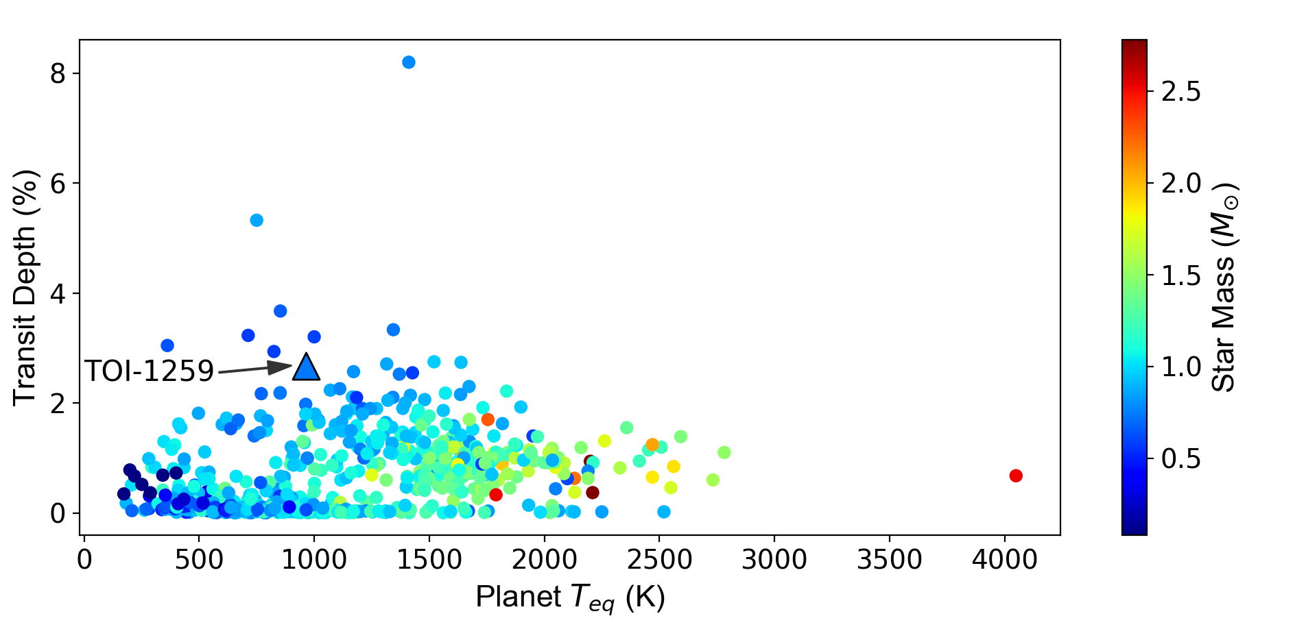
Figure 1: Transit depths of all confirmed transiting exoplanets as a function of the planet’s equilibrium temperature (where such a value has been calculated). The colour indicates the mass of the host star in solar masses. The triangle demarcates TOI-1259 with $2.7\%$ deep transits.

2 Observations

2.1 TESS photometry

The TESS mission observed TOI-1259 in 2-minute cadence mode for a total of $240$ days, covering nine sectors (14, 17–21, 24–26) between 18 July 2019 and 4 July 2020. The TESS Science Processing Operations Center (SPOC) pipeline (Jenkins et al., 2016) identified a $\sim 2.5\text{\,}\mathrm{\char 37\relax}$ transit signal lasting $\sim 2.2\text{\,}\mathrm{h}$, repeating with a period of $3.48\text{\,}\mathrm{d}$. The flat-bottomed shape and deep transit – combined with the K dwarf host – is consistent with a giant planet, substellar object, or very low-mass star. There were 58 transit events in the TESS data.

The TESS spacecraft fires its thrusters to unload angular momentum from its reaction wheels every few days, which may cause the images obtained in the timestamps to appear disjoint. To make sure the momentum dumps do not affect our further analysis, we identify the times of these events from the Data Quality Flags in the FITS files, and exclude the data obtained within four hours on either side of the thruster events.

2.2 Ground based follow-up photometry

We acquired ground-based time-series follow-up photometry of TOI-1259A as part of the TESS Follow-up Observing Program (TFOP). A full transit was observed on UTC 2019 October 10 using an unfiltered diffuser and again on UTC 2019 October 17 in $g^{\prime}$-band from the Deep Sky West 0.5-m telescope near Rowe, New Mexico, USA. An egress was observed on UTC 2019 October 6 in R- and V-band using two 0.4-m telescopes at Kourovka observatory of Ural Federal University near Yekaterinburg, Russia. A full transit was observed on UTC 2019 October 24 in $z^{\prime}$-band from the 0.36-m telescope at Acton Sky Portal private observatory in Acton, MA, USA. A full transit was observed on UTC 2019 December 4 in R-band from the 0.25-m telescope at Ananjev L33 private observatory near Ananjev, Ukraine. All observations detected on-time transits with depths consistent with TESS using apertures that were not blended with any known TICv8 or Gaia DR2 neighboring stars, except the diffuser observation was partially contaminated with a star that is too faint to cause the transit detection. Although TESS observed 58 transits of TOI-1259 b in Cycle 2, we also include all available ground-based light curves in our analysis, with the exception of the $R$- and $V$-band observations at Kourovka Observatory on 2019 October 6 which only observed the egress. The reduced data of all ground-based photometry are available at ExoFOP-TESS.

2.3 SOPHIE radial velocities

To measure the mass of TOI-1259Ab we used SOPHIE, which is a high resolution échelle spectrograph used to find extra-solar planets with high-precision RVs (Perruchot et al., 2008; Bouchy et al., 2009). It is installed on the 1.93 metre telescope at Observatoire de Haute Provence, France.

We obtained 19 RV measurements of TOI-1259Ab between June 10 2020 and July 16 2020 using the SOPHIE spectrograph. All RVs were calculated using the standard SOPHIE pipeline, where a Cross-Correlation Function (CCF) is calculated between the data and a K5 mask. Each observation yielded an RV with a precision of roughly 20$\rm m\,s^{-1}$.

We note that our spectra are not contaminated by the bound white dwarf, since it is both too faint (19.23 magnitude compared with 12.08 for the host star) and too far away (13.9 arcsec separation compared with 3 arcsec diameter SOPHIE fibres) to contribute any light.

2.4 Gaia Astrometry

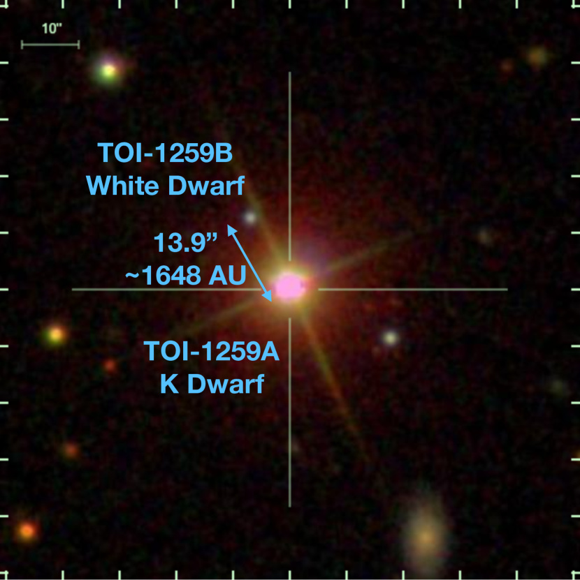
Figure 2: SDSS image of the planet host TOI-1259A and its bound white dwarf companion TOI-1259B. The image is centered on TOI-1259A at RA $18\text{<sup id="S2.F2.3.m1.1.1.2.2.3.1nest" class="ltx\_sup">h</sup>}⁤48\text{<sup id="S2.F2.3.m1.1.1.2.3.3.1nest" class="ltx\_sup">m</sup>}⁤24.\text{<sup id="S2.F2.3.m1.1.1.2.4.4.1nest" class="ltx\_sup">s</sup>}07$ , Dec $+79\mathrm{°}⁤15\mathrm{\prime }⁤21.\mathrm{″}76$.

TOI-1259A and its white dwarf companion (TOI-1259B) were identified as a candidate wide binary by El-Badry & Rix (2018), who searched Gaia DR2 for pairs of stars with positions, parallaxes, and proper motions consistent with bound Keplerian orbits. Figure 2 shows an SDSS image of the system, with both the K-dwarf primary and white dwarf companion clearly visible. The projected angular (physical) separation of the pair is 13.9 arcsec (1648 AU). The plane-of-the-sky absolute velocity difference between the WD and K dwarf is $\Delta V_{\perp}=0.47^{+0.59}_{-0.25}\,\,{\rm km\,s^{-1}}$. For comparison, we can calculate the Keplerian orbital velocity of a circular orbit separated by 1648 AU, with masses $0.68$ and $0.561M_{\odot}$ (see Table 3):

$$V=\sqrt{\frac{G\left(M_{\star}+M_{\rm WD}\right)}{{\rm sep}_{\rm WD}}},$$ (1)

where $G=6.67384\times 10^{-11}$. The value $V=0.82{\rm km\,s^{-1}}$ is consistent with the Gaia measurement, within the precision of the measurements which are limited by the Gaia proper motion uncertainties. The semi-major axis of the WD - K dwarf orbit and the 3D separation of the two stars are not currently measurable. However, for randomly oriented orbits and a plausible eccentricity distribution, the projected semi-major axis is almost always within a factor of two of the true semi-major axis (see El-Badry & Rix 2018, their Figure B1). The white dwarf companion was later independently identified by Mugrauer & Michel (2020).

Because orbital accelerations are not easy to measure in long-period binaries, distinguishing gravitationally bound wide binaries from chance alignments depends on statistical arguments about the probability of chance alignments. The chance alignment probability for a given separation, data quality, and background source density can be estimated empirically (e.g. Lépine & Bongiorno, 2007; El-Badry et al., 2019; Tian et al., 2020). We follow the approach described in Tian et al. (2020) to estimate the chance-alignment probability. In brief, we repeat the binary search after artificially shifting each star in Gaia DR2 by $\sim$1 degree, searching for companions around its new position. This procedure removes genuine binaries, but preserves chance alignment statistics (see Lépine & Bongiorno 2007). Comparing the number of binary candidates found so far to the number found in Gaia DR2 at similar separation, we estimate a chance-alignment probability of $\sim 1\times 10^{-4}$ for TOI-1259A and its companion. That is, there is little doubt that the planet host and white dwarf are physically associated.

3 Analysis and results

3.1 Host star parameters

We performed an analysis of the broadband spectral energy distribution (SED) of the star together with the Gaia DR2 parallaxes (adjusted by $+0.08$ mas to account for the systematic offset reported by Stassun & Torres, 2018), in order to determine an empirical measurement of the stellar radius, following the procedures described in Stassun & Torres (2016); Stassun et al. (2017); Stassun et al. (2018). We pulled the $BVgri$ magnitudes from APASS, the $JHK_{S}$ magnitudes from 2MASS, the W1–W4 magnitudes from WISE, the $GG_{\rm BP}G_{\rm RP}$ magnitudes from Gaia, and the NUV magnitude from GALEX. Together, the available photometry spans the full stellar SED over the wavelength range 0.2–22 $\mu$m (see Figure 3).

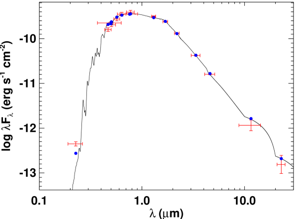
Figure 3: Spectral energy distribution of TOI-1259A. Red symbols represent the observed photometric measurements, where the horizontal bars represent the effective width of the passband. Blue symbols are the model fluxes from the best-fit Kurucz (1979) atmosphere model (black).

We performed a fit to the SED using Kurucz (1979) stellar atmosphere models, with the effective temperature ($T_{\rm eff}$), metallicity ([Fe/H]), surface gravity ($\log g$) as free parameters. The only additional free parameter is the extinction ($A_{V}$), which we restricted to the maximum line-of-sight value from the dust maps of Schlegel et al. (1998). The resulting fit is very good (Fig. 3) with a reduced $\chi^{2}$ of 1.7 and best-fit $A_{V}=0.20\pm 0.07$, $T_{\rm eff}=4775\pm 100$ K, $\log g=4.5\pm 0.5$, and [Fe/H] $=-0.5\pm 0.5$. Integrating the (unreddened) model SED gives the bolometric flux at Earth, $F_{\rm bol}=5.94\pm 0.14\times 10^{-10}$ erg s^-1 cm^-2. Taking the $F_{\rm bol}$ and $T_{\rm eff}$ together with the Gaia DR2 parallax, gives the stellar radius, $R_{\star}=0.739\pm 0.031$ R_⊙.

The stellar mass can be obtained from the SED analysis in two ways. First, we can use the $R_{\star}$ together with $\log g$ to obtain a mass estimate of $M_{\star}=0.79\pm 0.14$ M_⊙. Alternatively, we can apply the Torres et al. (2010) empirical mass-radius relations to get a value $M_{\star}=0.68\pm 0.08$ M_⊙.

As an independent test of our stellar parameters, we ran ExoFASTv2 (Eastman et al., 2019) to create a joint fit of the SED and two different types of isochrones: MIST (Dotter, 2016; Choi et al., 2016) and PARSEC (Bressan et al., 2012). With MIST we obtain $R_{\star}=0.733\pm 0.022$ and $M_{\star}=0.777^{+0.037}_{-0.038}$ and with PARSEC we obtain similar values of $R_{\star}=0.729\pm 0.020$ and $M_{\star}=0.777^{+0.034}_{-0.031}$.

Throughout this paper we will use the $R_{\star}=0.739R_{\odot}$ and $M_{\star}=0.68M_{\odot}$ values calculated using the empirical SED and Torres et al. (2010) relation, respectively. These are the priors that will be used in the global analysis to determine the planet parameters in Sect. 3.6.

Table 3: Stellar radius and mass measurements based on four different methods. In all cases we use a fit to the SED combined with Gaia DR2 parallaxes. In methods 1 and 2 we follow the procedure of Stassun & Torres (2016); Stassun et al. (2017); Stassun et al. (2018) to derive the radius and the mass comes from the SED measurement of the surface gravity $\log g$ (1) and the Torres et al. (2010) mass-radius relationship (2). In methods 3 and 4 we use ExoFASTv2 (Eastman et al., 2019) to fit the SED and two different isochrones. We use method 2 (in bold) as the nominal value.

Method	Radius	Mass
	($R_{\odot}$)	($M_{\odot}$)
1. SED + $\log g$	$0.739\pm 0.031$	$0.79\pm 0.14$
2. SED + Torres et al. (2010) M-R	$0.739\pm 0.031$	$0.68\pm 0.08$
3. SED + MIST isochrones	$0.733\pm 0.022$	$0.777^{+0.037}_{-0.038}$
4. SED + PARSEC isochrones	$0.729\pm 0.020$	$0.777^{+0.034}_{-0.031}$

3.2 Host star rotation

We use a Systematics-Insensitive Periodogram (SIP) to build a periodogram whilst simultaneously detrending TESS instrument systematics from scattered background, following the method first described in Angus et al. (2016) and more recently implemented for TESS data in Hedges et al. (2020). For this we use the SAP lightcurves, since the PDCSAP lightcurves tend to have the rotation period removed, or at least made harder to identify. The SIP power amplitude is shown in Figure  4. The SIP shows the most significant power at a period of P_rot=28 d and a secondary peak at P${}_{\rm rot}\approx$40 days. We adopt the more significant peak at P_rot=28 d as the true rotation rate of TOI-1259. The signal at P${}_{\rm rot}\approx$40 days is possibly an alias of the rotation period.

The rotation period of P_rot=28 d is close to the orbital period of TESS (27 days). We conduct two tests of the validity of this rotation rate. First, We construct SIPs for the targets neighboring TOI-1259 and find no evidence of a similar peak in near-by targets. Second, we create a SIP for all “background” pixels outside of the TESS pipeline aperture in the TESS Target Pixel File for TOI-1259. This background SIP, shown as a blue line in Fig. 4, has no power at 28 days. This suggests that the 28 day signal is intrinsic to the target, and not an artifact of, for example, the sampling frequency of TESS.

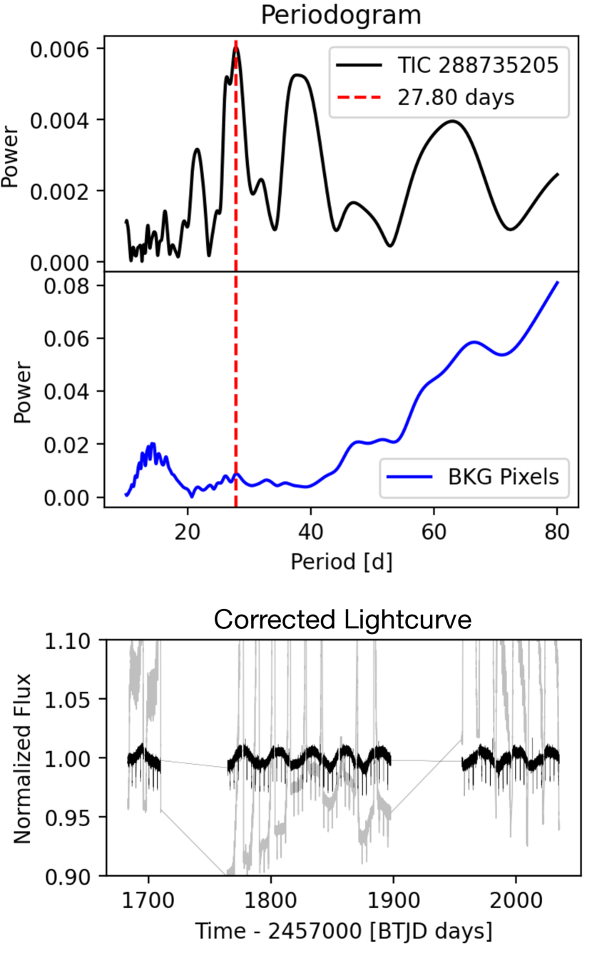
Figure 4: Top: Systematics-Insensitive Periodogram (SIP) for TOI-1259b. The periodogram is calculated for both the corrected lightcurve (black line) and the background (BKG) pixels (blue line). There is a strong peak in the SIP at 28 days, which is attributed to the rotation of the planet host and denoted by a red dashed line. The background pixels show no evidence of any periodicity, suggesting that the 28 day signal is both real and intrinsic to the target. Note that these periodograms are not normalized by the measurement errors. Bottom: The light curve for TOI-1259. Grey points show the raw data TESS data, and black points show the data corrected using tess-sip, showing a clear periodicity.

3.3 Host star age

When estimating the ages of K dwarfs using gyrochronology, it is essential to account for ‘stalled magnetic braking’. Recent observations have revealed that rotational evolution is inhibited for middle-aged K dwarfs (Curtis et al., 2019; Angus et al., 2020). This stalled rotational evolution is thought to be caused by an internal redistribution of angular momentum (Spada & Lanzafame, 2020). Unless this phenomenon is taken into account, the ages of K dwarfs could be underestimated by more than 2 Gyr.

We estimated an age for this star using a new gyrochronology model that accounts for stalled magnetic braking (Angus et al., in prep). This model was calibrated by fitting a Gaussian process, a semi-parametric model that is flexible enough to capture the complex nature of stellar spin-down, to a number of asteroseismic stars and open clusters, including NGC 6811 where many member stars exhibit stalled magnetic braking (Curtis et al., 2019). We also used kinematic ages of Kepler field stars to calibrate this model for old K and early M dwarfs, where there is a dearth of suitable open cluster calibration stars. These kinematic ages also reflect the stalled magnetic braking behaviour seen in open clusters (Angus et al., 2020).

Using this model, we infer an age of 4.8${}^{+0.7}_{-0.8}$ Gyr for this star. The quoted age uncertainty is the formal uncertainty that results from the uncertainty on the star’s rotation-period, and does not account for uncertainty in the model. Quantifying the magnitude of the model-uncertainty is beyond the scope of this paper, however a 20% uncertainty of around 1 Gyr may be a more reasonable estimate of the true age-uncertainty. This estimated age for the planet host is consistent with that of the total age of the white dwarf (Sect. 3.4).

3.4 White dwarf age

White dwarfs (WDs) steadily cool as they age. A WD’s cooling age – that is, the time since it became a WD – can therefore be constrained from its temperature and luminosity. If the WD’s mass is known, the initial mass of its progenitor star can be inferred through the initial-final mass relation (IFMR), and this initial mass constrains the pre-WD age of the WD progenitor. Therfore if we have a well-constrained distance to the WD then its total age, i.e. the sum of its main sequence lifetime and its cooling age, can be robustly measured from its spectral energy distribution (SED). Under the reasonable ansatz that the WD and K dwarf formed at the same time, we can then measure the total system age from the WD.

We use BASE-9 (von Hippel et al., 2006; De Gennaro et al., 2008; Stein et al., 2013; Stenning et al., 2016) to fit the SDSS $ugriz$ photometry of the the WD. BASE-9 combines evolutionary models for WDs (Althaus & Benvenuto, 1998; Montgomery et al., 1999), WD atmospheric models (Bergeron et al., 1995; Holberg & Bergeron, 2006), PARSEC evolutionary models (Bressan et al., 2012), and semi-empirical IFMRs to predict the SED of a WD with a given age, initial mass and metallicity, distance, extinction, and spectral type. It then uses MCMC methods to constrain these parameters from the SED of an observed WD.

We use the Gaia parallax of the brighter K dwarf companion as a prior. For the initial [Fe/H], we assume a Gaussian prior with a mean of -0.2 and a standard deviation of 0.3, appropriate for a disk star in the solar neighborhood (e.g. Hayden et al., 2015). The spectral type of the WD is not known. Although we expect extinction to be almost negligible for such a nearby WD, we fit the extinction $A_{V}$ as a free parameter, with a Gaussian prior with a mean of 0.01 and a standard deviation of 0.02, based on the 3D dust map of Green et al. (2019). For context, the SFD reddening (which quantifies the total dust column to infinity, including dust behind the WD) at the WD’s position is $E(B-V)=0.085$ (Schlegel et al., 1998). We use a flat prior between 0 and 12 Gyr for total age. Our fiducial fit assumes the WD has a hydrogen atmosphere, which is true for $\sim$75% of WDs with its temperature and mass. We also show how the constraints would change if the WD has a helium atmosphere in Table 4.

A systematic uncertainty in modeling the WD’s evolution is the IFMR. Because most published IFMRs are discrete, analytic fitting functions, this uncertainty is difficult to marginalize over gracefully. To estimate the magnitude of this uncertainty, we compare constraints that assume two different IFMRs: the IFMR measured by Williams et al. (2009) from bound clusters, and the IFRM measured by El-Badry et al. (2018) from the Gaia color-magnitude diagram of nearby field WDs.

Table 4: Parameters of the WD. We compare constraints derived assuming a hydrogen versus helium atmosphere, and constraints that assume two different IFMRs.

Parameter	H atm; El-Badry+18 IFMR	H atm; Williams+09 IFMR	He atm; El-Badry+18 IFMR	He atm; Williams+09 IFMR
Total age (Gyr)	$4.08^{+1.21}_{-0.53}$	$3.73^{+0.56}_{-0.31}$	$4.67^{+1.70}_{-0.94}$	$3.94^{+0.81}_{-0.44}$
Cooling age (Gyr)	$1.88^{+0.07}_{-0.06}$	$1.88^{+0.07}_{-0.06}$	$1.78^{+0.06}_{-0.05}$	$1.78^{+0.06}_{-0.05}$
Pre-WD age (Gyr)	$2.18^{+1.2733}_{-0.5597}$	$1.84^{+0.61}_{-0.35}$	$2.87^{+1.73}_{-1.00}$	$2.14^{+0.86}_{-0.47}$
Radius ($R_{\odot}$)	$0.0131^{+0.0003}_{-0.0003}$	$0.0131^{+0.0003}_{-0.0003}$	$0.0129^{+0.0003}_{-0.0003}$	$0.0129^{+0.0003}_{-0.0003}$
Mass ($M_{\odot}$)	$0.561^{+0.021}_{-0.021}$	$0.561^{+0.021}_{-0.021}$	$0.548^{+0.021}_{-0.019}$	$0.548^{+0.021}_{-0.019}$
Initial mass ($M_{\odot}$)	$1.59^{+0.22}_{-0.22}$	$1.72^{+0.17}_{-0.17}$	$1.45^{+0.22}_{-0.20}$	$1.61^{+0.17}_{-0.17}$
$T_{\rm eff}$ (K)	$6300^{+80}_{-70}$	$6300^{+80}_{-70}$	$6330^{+80}_{-70}$	$6330^{+80}_{-70}$
$A_{V}$ (mag)	$0.019^{+0.018}_{-0.013}$	$0.019^{+0.018}_{-0.013}$	$0.019^{+0.017}_{-0.013}$	$0.019^{+0.017}_{-0.013}$

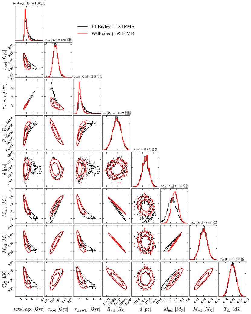
Figure 5: Parameters of the WD and its progenitor, obtained from fitting the SED. We compare constraints obtained when assuming the initial-final mass relations (IFMR) from El-Badry et al. (2018) and Williams et al. (2009). For this figure we assume a hydrogen atmosphere, but in Table 4 we also show results for a potential helium atmosphere. Values listed on the diagonal are based on the El-Badry et al. (2018) IFMR. Contours enclose 68 and 95% probability. The total age of the WD – and thus, presumably, the age of the system – is at least 3 Gyr. The age uncertainty is dominated by uncertainty in the mass and pre-WD age of the progenitor.

Figure 5 shows the resulting constraints on parameters of the WD, assuming a hydrogen atmosphere. Values are also reported in Table 4. The temperature and radius of the WD are well-constrained by the SED. Because the radius of a WD is determined primarily by its mass, this also constrains the WD’s mass, which in turn constrains the initial mass of the WD progenitor. The cooling age of the WD is reasonably well-constrained to be between 1.7 and 2 Gyr. The pre-WD age is more uncertain, because a modest uncertainty in initial mass leads to a significant uncertainty in main-sequence lifetime. This is the primary cause of the differences in the constraints obtained for the two different IFMRs. The two relations are actually quite similar at the relevant WD mass (see El-Badry et al. 2018, their Figure 3), but the El-Badry et al. (2018) relation is somewhat shallower. This means that a larger range of initial masses could produce the observed WD mass, and thus, that there is a larger range of allowed pre-WD ages. The pre-WD lifetime of a $2M_{\odot}$ star is $\approx 1.3$ Gyr, while that of a $1.2M_{\odot}$ star is $\approx 6$ Gyr, so the resulting uncertainty is non-negligible. A tighter constraint on the WD mass – which is potentially achievable via gravitational redshift; e.g. Reid 1996 – could improve the statistical uncertainty on total age. However, the constraint is already tight enough that systematic uncertainty due to the IFMR is comparable to the statistical uncertainty, so the IFMR uncertainty would likely dominate the age uncertainty even with significantly better data.

Table 4 also shows how constraints on the WD’s parameters would change if it had a helium atmosphere rather than a hydrogen atmosphere. Changing the atmosphere slightly changes the WD’s colors and the mass-radius relation, such that the implied mass of the WD is lower. The difference is, however, relatively modest. Obtaining a spectrum of the WD would remove this source of uncertainty, since a WD with a hydrogen atmosphere and $T_{\rm eff}>6000$ K would have detectable Balmer lines.

Our derived total age for TOI-1259B is consistent with the 4.8${}^{+0.7}_{-0.8}$ Gyr age derived for the planet host TOI-1259A based on gyrochronology (Sect. 3.3).

3.5 Radial velocity modelling

To confirm the planet we conduct two independent analyses. First, in this section we detect solely the RV signal, using the genetic algorithm Yorbit (Ségransan et al., 2010). Second, in Sect. 3.6 we do a combined fit of both the photometry and RV, with a completely different code.

In Fig. 6 we show a Generalized Lomb-Scargle periodogram derived solely from the SOPHIE RVs. The 3.478 day period from the TOI catalogue is denoted by a red dashed line. This corresponds to the highest peak in the periodogram, demonstrating that the RV signal is produced by the same body that produces the TESS transit signals. We note that our spectra are not contaminated by the bound white dwarf, since it is both too faint (19.23 magnitude compared with 12.08 for the host star) and too far away (13.9 arcsec separation compared with 3 arcsec diameter SOPHIE fibres) to contribute any light.

We then run the Yorbit genetic algorithm, allowing it to fit a single Keplerian model with a period between 3 and 4 days, which is roughly centered on the highest peak of the periodogram. The best-fitting model of the RVs alone has a period of $P_{\rm pl}=3.42\pm 0.06$ days, and a best-fitting transit mid point of $2037.96\pm 0.14$ (BJD_UTC - 2 457 000), both of which match the TESS photometry. The best-fitting model also has an eccentricity of $e_{\rm pl}=0.178$, which would be surprisingly high for such a short period planet.

To test if the planet signal (and its potential eccentricity) is significant, we calculate the Bayesian Information Criterion ($BIC$) by

$$BIC=n\ln\left(\frac{RSS}{n}\right)+k\ln{n_{\rm obs}},$$ (2)

where $k$ is the number of model parameters, $RSS$ is the sum of the squares of the model residuals (in $m/s$) and $n_{\rm obs}=13$ is the number of observations. We calculate the BIC for a flat line ($k=1$), the best fitting eccentric model from Yorbit ($k=6$) and a forced circular model with the same period ($k=4$). The flat, eccentric and circular $BIC$ values are 157.8, 136.2 and 133.6, respectively. The circular planet model has the lowest $BIC$, making it the favoured model. For one model to be significantly better than another though, a $BIC$ reduction of more than 6 is considered “strong evidence”. This means that the circular model is not significantly better than the eccentric model, but both are significantly better than the flat model. Otherwise said, the RVs alone provide strong evidence that the planet exists, but we cannot constrain its eccentricity.

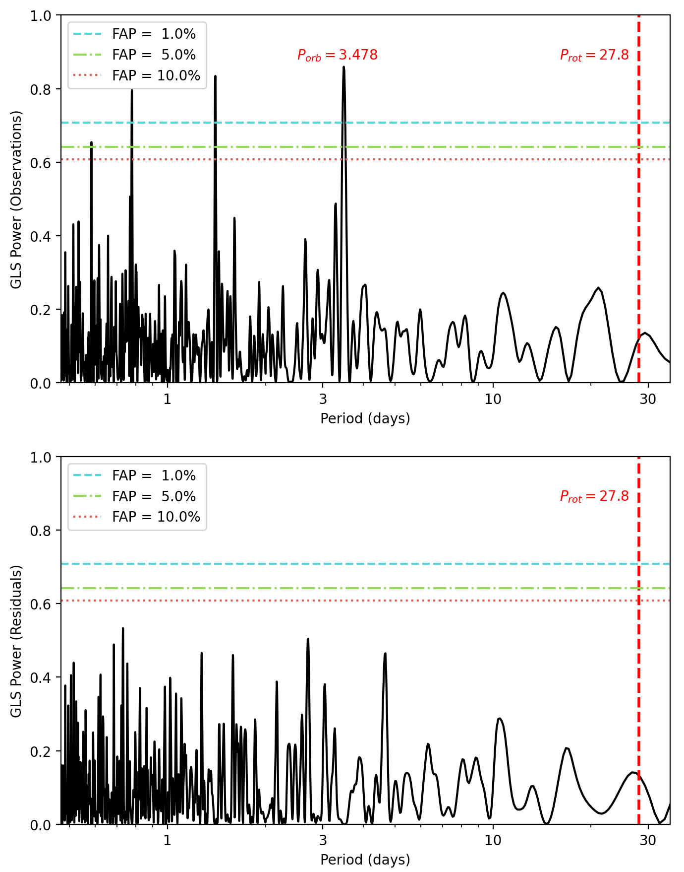
Figure 6: Generalized Lomb-Scargle (GLS) periodogram of the 19 SOPHIE RV points (top) and the residuals to the circular Keplerian fit (bottom). The highest peak for the observations corresponds to the transiting planet orbital period at 3.45 days. There are also harmonics at integer fractions of this period. Note that these periodogram does not include any information from the photometry. The RV detection alone is significant, above a 1% false alarm propbability (FAP). For reference, we show the 27.8 day rotation period of the host star with a red dashed line, at which there is no power in the GLS. The GLS periodogram of the residuals shows no significant peak above a 10% FAP.

3.6 Global modelling of the photometry and radial velocity

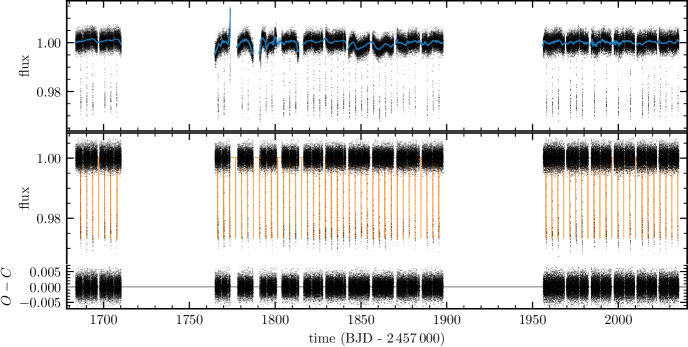
Figure 7: Upper panel: Nine sectors of TESS PDCSAP photometry of TOI-1259. The blue model is the Gaussian process model. Middle panel: The light curve after removing the Gaussian process model, showing transits only, with the transit model overlaid in orange. Bottom panel: Residuals from the best-fitting full model.

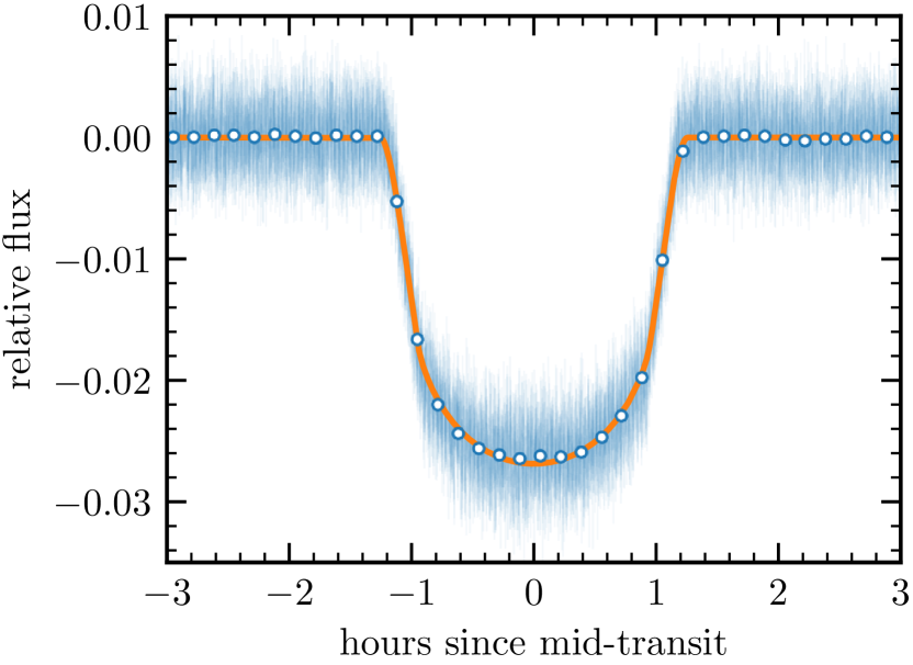
Figure 8: Phase folded and detrended light curve of the primary transit after removing the Gaussian process model. We show the unbinned data in blue, and the data averaged in $10\text{\,}\mathrm{min}$ bins in blue/white points. The orange line is the best-fitting transit model, with a maximum depth of 2.7%.

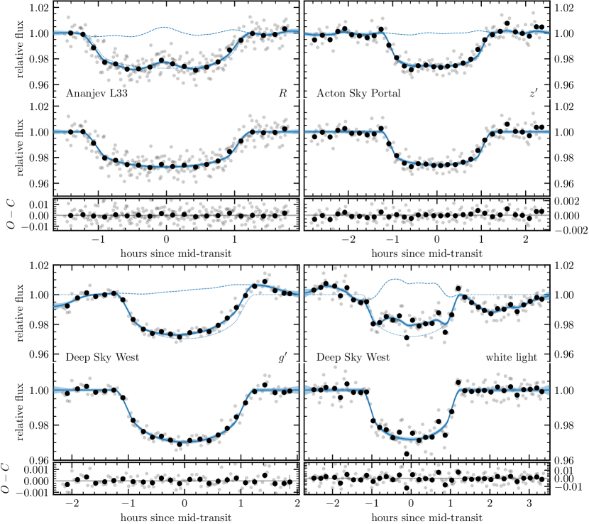
Figure 9: Transit light curves of TOI-1259 b followed up with small ($<50\,$cm) ground-based telescopes with various filters. For each light curve, we show the raw data in the top panel (grey) overlaid with data binned in 10 min intervals (black). The best-fitting model is shown as a solid blue line, which consists of a Gaussian process (GP) model (dashed) and transit model (dotted). The $1\sigma$ uncertainty of the GP model is indicated by the shaded region. The middle panels are “cleaned” light curves after removing the GP model, and the bottom panels are residuals from the best-fitting model.

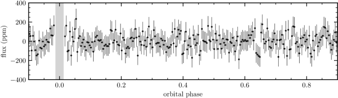
Figure 10: Top: The light curve folded on the phase of the planet orbit, with data points binned in $20\text{\,}\mathrm{min}$ intervals. The grey highlighted area is the transit duration. The expected secondary eclipse depth is $63\text{\,}\mathrm{ppm}$, which is comparable to the noise. There is no apparent signal at $\phi=0.5$, where one could expect a secondary eclipse for a circular orbit. There is a tentative signal centered on $\phi=0.64$ with a duration that is consistent with a secondary eclipse, however this implies an eccentricity of roughly $0.20.3\text{\,}$ which is incompatible with the RV data.

We model the combined light curves (TESS and ground-based) and RV data using exoplanet (Foreman-Mackey et al., 2020). The exoplanet software uses starry (Luger et al., 2019; Agol et al., 2020) to rapidly compute analytical limb darkened light curves, and is also integrated with celerite for scalable Gaussian process computations. Since the models (and their gradients) within exoplanet are analytical, the software is built on the Theano (Theano Development Team, 2016) engine and therefore allows the use of pymc3 (Salvatier et al., 2016), which offers fast and effective convergence using gradient-based sampling algorithms.

The Simple Aperture Photometry (SAP) light curve from TESS shows a clear rotational signal of the host star (Fig. 4). While we could take advantage of the rotational signal in our transit modelling, we derive a rotation period in Section 3.2 using the Systematics-Insensitive Periodogram (SIP). We therefore opt to use the PDCSAP flux (Stumpe et al., 2012; Smith et al., 2012; Stumpe et al., 2014; Jenkins et al., 2016). in our transit analysis, which is corrected for spacecraft systematics and the rotation signal since the derived rotation period is on a similar timescale to a TESS sector.

The TESS spacecraft fires its thrusters to unload angular momentum from its reaction wheels every few days, which may cause the images obtained in the timestamps to appear disjoint. To make sure the momentum dumps do not affect our further analysis, we identify the times of these events from the Data Quality Flags in the FITS files, and exclude the data obtained within four hours on either side of the thruster events.

We model the out-of-transit variability using Gaussian processes (GPs). We use the SHOTerm model in celerite (Foreman-Mackey et al., 2017; Foreman-Mackey, 2018), fixing the quality factor $Q=1/\sqrt{2}$ so that the covariance function becomes

$$k(\tau)=S_{0}\,\omega_{0}\,\exp{\left(-\frac{1}{\sqrt{2}}\omega_{0}\tau\right)}\cos{\left(\frac{\omega_{0}\,\tau}{\sqrt{2}}-\frac{\pi}{4}\right)}.$$

We fit for the natural logarithms of the amplitude and frequency, $S_{0}$ and $\omega_{0}$. Since each TESS sector may have systematics on different timescales and amplitudes, we model each sector and ground-based light curve with individual GPs, and also assign individual flux scaling terms and white noise terms.

We fit the TESS and ground-based photometry using our Gaussian process model combined with a transit model, as well as a Keplerian model for the RV data. We place Gaussian priors on the stellar mass and radius using values from the SED analysis in Section 3.1, $M_{\star}=$0.68\pm 0.08\text{\,}\mathrm{M_{\odot}}$$, $R_{\star}=$0.739\pm 0.031\text{\,}\mathrm{R_{\odot}}$$. Further, we vary the impact parameter $b$, as well as the natural logarithms of the period $P$, mid-transit time $T_{0}$, planet radius $R_{\mathrm{pl}}$, and planet mass $M_{\mathrm{pl}}$. The limb darkening of the star is described by a quadratic formula, with coefficients and uncertainties within the TESS, $R$, $z^{\prime}$, $g^{\prime}$, and white light bands determined using pyldtk (Parviainen & Aigrain, 2015) and exofast online tool. pyldtk and exofast interpolate the Husser et al. (2013) and Claret & Bloemen (2011) atmospheric models, respectively, where we used stellar parameters from Table 3. We vary the limb darkening coefficients with a Gaussian prior centered on the computed values, with standard deviation of $0.01$ and $0.02$ for $c_{1}$ and $c_{2}$, respectively. These uncertainties roughly correspond to twice the computed error, which we inflated to account for uncertainties in the stellar atmospheric models. The SOPHIE RV data is further described by the semi-amplitude $K$, eccentricity parameters $\sqrt{e}\cos{\omega}$ and $\sqrt{e}\sin{\omega}$, and additional nuisance parameters that model the offset and a white noise term that is added in quadrature to the SOPHIE uncertainties.

We first perform a maximum likelihood fit, followed by MCMC sampling using the NUTS sampler within pymc3 to obtain credible intervals on our parameters. We launch two independent chains that are run for 4000 tuning steps and 2000 production steps. We confirmed that the sampler converged by checking the Gelman-Rubin criterion, $\hat{R}<1.01$, and all parameters have $>200$ effective samples. We report the values and $15.8$ and $84.2$ percentiles for the stellar, planet and orbital parameters in Table 5, and similarly for the nuisance parameters in Table 6. The fits to the transit photometry is shown in Fig. 7,8,9, and the RV fit in Fig. 11. Our RV measurements are all published online.

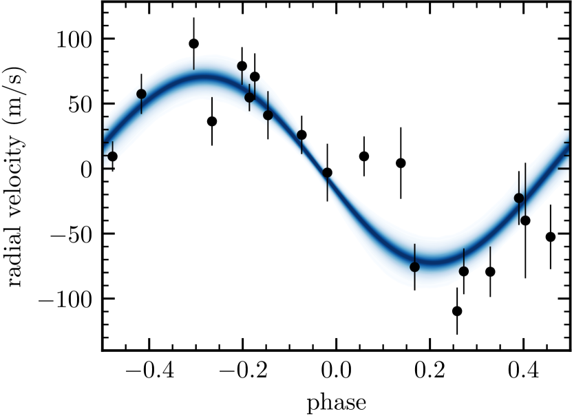
Figure 11: SOPHIE RV (black) with the 99^th percentile models from a joint fit with the TESS photometry encapsulated in the blue region. The RV are indicative of a $0.44M_{\rm Jup}$ planet, and are in phase with the transits observed by TESS.

Table 5: Derived parameters from the joint modelling of TESS photometric and SOPHIE RV data. ^aControlled by Gaussian prior, $\mathcal{N}(0.68,0.05)$. ^bControlled by Gaussian prior, $\mathcal{N}(0.739,0.031)$. ^cAssuming zero albedo.

Parameter	Description	Value	Value
		circular model (adopted)	eccentric model
Derived stellar parameters
$M_{\star}$ ($\mathrm{M_{\odot}}$)	Stellar massa	$0.744^{+0.064}_{-0.059}$	$0.743^{+0.066}_{-0.064}$
$R_{\star}$ ($\mathrm{R_{\odot}}$)	Stellar radiusb	$0.711^{+0.020}_{-0.019}$	$0.711^{+0.024}_{-0.024}$
$\rho_{\star}$ ($\mathrm{g}\text{\,}{\mathrm{cm}}^{-3}$)	Stellar density	$2.92^{+0.03}_{-0.04}$	$2.91^{+0.26}_{-0.25}$
$\log{g_{\star}}$ (cgs)	Stellar surface gravity	$4.605^{+0.013}_{-0.013}$	$4.581^{+0.044}_{-0.045}$
Derived planet parameters
$P$ (days)	Orbital period	$3.4779780^{+0.0000019}_{-0.0000017}$	$3.4779779^{+0.0000018}_{-0.0000016}$
$T_{0}$ (BJDUTC - $2\,457\,000$)	Transit mid-point	$1686.700531^{+0.000097}_{-0.000104}$	$1686.700536^{+0.000099}_{-0.000100}$
$M_{\text{pl}}$ ($\mathrm{M_{\text{Jup}}}$)	Planet mass	$0.441^{+0.049}_{-0.047}$	$0.440^{+0.051}_{-0.047}$
$R_{\text{pl}}$ ($\mathrm{R_{\text{Jup}}}$)	Planet radius	$1.022^{+0.030}_{-0.027}$	$1.021^{+0.034}_{-0.034}$
$\rho_{\text{pl}}$ ($\mathrm{g}\text{\,}{\mathrm{cm}}^{-3}$)	Planet density	$0.513^{+0.051}_{-0.048}$	$0.513^{+0.071}_{-0.066}$
$\log{g_{\text{pl}}}$ (cgs)	Planet surface gravity	$3.019^{+0.040}_{-0.040}$	$3.019^{+0.050}_{-0.053}$
$M_{\text{pl}}/M_{\star}$	Mass ratio	$0.000567^{+0.000056}_{-0.000055}$	$0.000568^{+0.000052}_{-0.000051}$
$R_{\text{pl}}/R_{\star}$	Planet-to-star radius ratio	$0.14762^{+0.00035}_{-0.00030}$	$0.14764^{+0.00032}_{-0.00031}$
$a/R_{\star}$	Scaled separation	$12.314^{+0.036}_{-0.056}$	$12.301^{+0.352}_{-0.358}$
$R_{\star}/a$	Scaled stellar radius	$0.08121^{+0.00037}_{-0.00023}$	$0.08130^{+0.00244}_{-0.00226}$
$R_{\text{pl}}/a$	Scaled planet radius	$0.011981^{+0.000077}_{-0.000033}$	$0.012002^{+0.000371}_{-0.000348}$
$T_{\mathrm{eq}}$ ($\mathrm{K}$)	Planet equilibrium temperaturec	$963^{+21}_{-21}$	$963^{+25}_{-25}$
$b$ ($R_{\star}$)	Impact parameter	$0.065^{+0.055}_{-0.044}$	$0.064^{+0.055}_{-0.045}$
$i_{\text{p}}$ ($\mathrm{\SIUnitSymbolDegree}$)	Orbital inclination	$89.70^{+0.20}_{-0.26}$	$89.70^{+0.21}_{-0.26}$
$a$ (AU)	Semi-major axis	$0.04070^{+0.00114}_{-0.00110}$	$0.04069^{+0.00116}_{-0.00120}$
$D_{T_{0}}$	Transit depth at $T_{0}$	$0.026759^{+0.000099}_{-0.000100}$	$0.026756^{+0.000097}_{-0.000095}$
$T_{14}$ (days)	Transit duration between $1\textsuperscript{st}$ and $4\textsuperscript{th}$ contacts	$0.10314^{+0.00020}_{-0.00020}$	$0.10313^{+0.00020}_{-0.00019}$
$K$ ($\mathrm{m}\text{\,}{\mathrm{s}}^{-1}$)	RV semi-amplitude	$72.0^{+6.8}_{-6.4}$	$72.2^{+6.4}_{-6.4}$
$e$	Eccentricity	$0$	$0.030^{+0.034}_{-0.022}$
$\omega$ ($\mathrm{\SIUnitSymbolDegree}$)	Argument of periastron	–	$5^{+132}_{-138}$
$\sqrt{e}\cos{\omega}$	Unit eccentricity parameter	–	$-0.038^{+0.142}_{-0.127}$
$\sqrt{e}\sin{\omega}$	Unit eccentricity parameter	–	$0.005^{+0.144}_{-0.156}$
$u_{\mathrm{TESS}}$	Limb darkening coefficient, TESS band	$0.5241^{+0.0066}_{-0.0064}$	$0.5232^{+0.0067}_{-0.0068}$
$v_{\mathrm{TESS}}$	Limb darkening coefficient, TESS band	$0.088^{+0.016}_{-0.017}$	$0.088^{+0.015}_{-0.015}$
$u_{R}$	Limb darkening coefficient, $R$ band	$0.5328^{+0.0103}_{-0.0097}$	$0.5333^{+0.0099}_{-0.0098}$
$v_{R}$	Limb darkening coefficient, $R$ band	$0.171^{+0.020}_{-0.020}$	$0.172^{+0.020}_{-0.020}$
$u_{z^{\prime}}$	Limb darkening coefficient, $z^{\prime}$ band	$0.3689^{+0.0102}_{-0.0097}$	$0.3687^{+0.0100}_{-0.0096}$
$v_{z^{\prime}}$	Limb darkening coefficient, $z^{\prime}$ band	$0.209^{+0.020}_{-0.020}$	$0.209^{+0.021}_{-0.020}$
$u_{g^{\prime}}$	Limb darkening coefficient, $g^{\prime}$ band	$0.8026^{+0.0098}_{-0.0101}$	$0.8024^{+0.0100}_{-0.0098}$
$v_{g^{\prime}}$	Limb darkening coefficient, $g^{\prime}$ band	$0.030^{+0.020}_{-0.021}$	$0.029^{+0.021}_{-0.020}$
$u_{\mathrm{white}}$	Limb darkening coefficient, white light	$0.6640^{+0.0098}_{-0.0100}$	$0.6627^{+0.0105}_{-0.0104}$
$v_{\mathrm{white}}$	Limb darkening coefficient, white light	$0.059^{+0.019}_{-0.019}$	$0.062^{+0.021}_{-0.020}$

The combined fit to the TESS light curves and SOPHIE RVs reveals that TOI-1259 b is a giant planet with mass $M_{\mathrm{pl}}=0.441^{+0.049}_{-0.047}\,$\mathrm{M_{\text{Jup}}}$$, and radius $R_{\text{pl}}=1.022^{+0.030}_{-0.027}\,$\mathrm{R_{\text{Jup}}}$$. The RV data constrains the eccentricity to be ${<}0.13$ ($99\%$ credible interval). Using the approximate tidal circularization timescale in §6 of Barker & Ogilvie (2009) with their example tidal parameters, we find that TOI-1259 b might have circularized after ${\sim}2\,$Gyr, which is shorter than the estimated age of the host star (${\sim}5\,$Gyr). As in Section 3.5, the eccentricity measurement from our global analysis is not statistically signficant. The BIC prefers a circular model over the eccentric model, with $\Delta\mathrm{BIC}=\mathrm{BIC}_{\mathrm{circ}}-\mathrm{BIC}_{\mathrm{ecc}}=-23.8$. We therefore adopt the circular model, but report results from both analyses in Table 5.

We visually searched for a secondary eclipse in the binned residuals of the phase-folded TESS photometry, shown in Fig. 10. The residuals close to phase 0.5 (where a secondary eclipse would be for a circular orbit) show no signs of a planet occultation. There may be a tentative signal of a $\sim 100\text{\,}\mathrm{ppm}$ secondary eclipse at phase $\sim 0.64$. However, this implies an eccentricity of roughly $0.20.3\text{\,}$. Such high eccentricities are not supported by the current RV data. We estimate the secondary eclipse depth to be 63 ppm, using the simple approximation $\approx 0.5(R_{\rm pl}/a_{\rm pl})^{2}$, where we assume a geometric albedo of 0.5 and ignore thermal emission. An eclipse of this depth would be consistent with the small dip seen at phase 0.64, but more observations, potentially including those from an extended TESS mission, would be needed to confirm that this feature is a secondary eclipse.

4 Discussion

We have confirmed that the TESS transiting candidate TOI-1259Ab is a 0.441$M_{\rm Jup}$ transiting exoplanet on a 3.48 day orbit, through our RV and ground-based photometric follow-up. Furthermore, by combining with the existing Gaia binaries catalog of El-Badry & Rix (2018), we show that this planet exists in a binary star system, where its primary star is a $0.68M_{\odot}$ K-dwarf and the secondary star is a $0.56M_{\odot}$ white dwarf on a bound orbit. The current projected separation is roughly 1648 AU. All of the key parameters of this system are summarised in Table 3.

4.1 Comparison with Mugrauer & Michel (2020)

Mugrauer & Michel (2020) independently characterised the white dwarf companion to TOI-1259. They also concluded that it was a bound companion, and determined a projected separation of roughly 1600 AU, which is the same as in El-Badry & Rix (2018). Their derived white dwarf effective temperature of $T_{\rm eff}=6473^{+672}_{-419}$ K agrees with our calculations of $T_{\rm eff}=6300^{+80}_{-70}$ K.

4.2 Dynamical history

Wang et al. (2014) determined that the planet frequency in binary systems was lower than that around single stars for binary separations up to 1500 AU. Some other studies suggest that the influence of a binary is less far-reaching, with only  100-200 AU and tighter binaries affecting planet populations (Kraus et al., 2016; Moe & Kratter, 2019; Ziegler et al., 2021). With a mass of $0.56M_{\odot}$ at a distance of about 1600 AU, our white dwarf is presently at a separation not predicted to impact planet formation. However, during its main sequence lifetime, the white dwarf’s progenitor would have been both more massive ($\sim 1.59M_{\odot}$) and much closer ($\sim 900$ AU, assuming adiabatic mass loss). At this point secular effects such as Kozai-Lidov (Lidov, 1962; Kozai, 1962; Mazeh & Shaham, 1979) may have been relevant to the planet. Indeed, the Kozai-Lidov effect may have brought the planet to its current orbital configuration, by inducing high-eccentricity tidal migration (Fabrycky & Tremaine, 2007; Naoz et al., 2012; Naoz, 2016), if the planet started out at a wider orbit, as would be expected for a gas giant. Given the estimated pre-white dwarf age of the system ($~{}2$ Gyr), a large range of orbital parameters could have led to the observed orbit of the planet TOI-1259Ab. In such a case, the companion star evolving into a white dwarf may have also acted as a natural “shutoff” for such secular effects (Dawson & Johnson, 2018).

We also note here that our combined photometry and RV fit favours a circular solution for the planetary orbit. The planet may have had a higher eccentricity (e.g. due to Kozai-Lidov) in the past but with a semi-major axis of only $0.04$ AU it likely would have been circularized by tidal interactions within the age of the system. Higher precision photometric follow-up that is able to reveal the secondary transit of the planet would most likely be the best means of detecting any potential small but non-zero eccentricity.

Any planets that orbited the white dwarf progenitor may have experienced the opposite effect; the evolution of their host into a white dwarf may have acted to “turn on” secular effects (Shappee & Thompson, 2013; Stephan et al., 2017, 2018, 2020a). This could cause the destruction of its planets. TOI-1259A’s white dwarf companion would therefore be a worthwhile target for finding signatures of heavy element pollution by planetary debris. In any case, more detailed studies of the dynamical history of TOI-1259 and of Gliese-86b, which has a white dwarf companion at a projected separation of just 21 AU (Queloz et al., 2000; Els et al., 2001; Lagrange et al., 2006), are warranted and will be part of a future work.

4.3 Future spectroscopic characterisation of the white dwarf companion

There is a propensity for white dwarfs to have atmospheres contaminated by heavy elements (Debes et al., 2012; Farihi, 2016; Wilson et al., 2019), despite an expectation that such elements would quickly settle towards the core due to the high gravity. This has been measured in white dwarfs without any known exoplanet companions, but the pollution itself has been attributed to the accretion of surrounding planetary material. It would be interesting to know if WD such as TOI-1259B, which do have a known associated planet, are more likely to be polluted than “lonely” WDs. Southworth et al. (2020) most recently tested this for WASP-98, but their spectroscopy of the white dwarf revealed a featureless spectrum and hence no evidence of pollution could be ascertained. It will ultimately be beneficial to conduct such spectroscopy on not only TOI-1259B, but indeed all of the similar systems listed in Table 2.

Follow-up spectroscopy will also hopefully inform us if the atmosphere is hydrogen- or helium-dominated. Breaking this degeneracy would allow a more accurate constraint on the WD parameters, since we could choose the appropriate model from Table 4.

4.4 Future JWST observations

Kempton et al. (2018) derived a Transmission Spectroscopy Metric (TSM). It is a means of prioritizing exoplanets for future atmospheric characterisation, in particular using the James Webb Space Telescope, and is proportional to the expected signal to noise ratio for the planet’s transmission spectrum. Their analytic expression is

$${\rm TSM}=S\times\frac{R_{\rm pl}^{3}T_{\rm eq}}{M_{\rm pl}R_{\star}^{2}}\times 10^{-m_{\rm J}/5},$$ (3)

where $m_{\rm J}$ is the magnitude of the host star in the J band and $S$ is a an empirical scale factor derived by Kempton et al. (2018) to make their simple analytic expression match the more detailed simulations of Louie et al. (2018). The factor $S$ depends on the radius of the transiting planet: $S=0.19$ for $R_{\rm pl}<1.5R_{\oplus}$; $S=1.26$ for $1.5<R_{\rm pl}<2.75R_{\oplus}$; $S=1.28$ for $2.75<R_{\rm lp}<4.0R_{\oplus}$ and $S=1.15$ for $R_{\rm pl}>4.0R_{\oplus}$.

For TOI-1259Ab we calculate a value of TSM $=180$, which places it in the top 3% of all confirmed transiting exoplanets. We demonstrate this in Fig. 12. TOI-1259Ab has a scaled separation $a/R_{\star}=12.314^{+0.036}_{-0.056}$ and an equilibrium temperature $T_{\rm eq}=963\pm 21$ K. Most of the planets with a higher TSM value are hotter and larger. There are only two objects cooler than 1000 K with a higher TSM: WASP-69b and WASP-107b. These two planets have already received considerable attention with respect to their atmospheres. WASP-69b (Anderson et al., 2014) has a confirmed presence of helium in its atmosphere from ground-based observations (Nortmann et al., 2018). WASP-107b (Anderson et al., 2017) is a so-called “super-puff”, based on a $0.12M_{\rm Jup}$ mass and a $0.94R_{\rm Jup}$ radius, and Hubble Space Telescope observations have revealed the presence of both helium (Spake et al., 2018) and water (Kreidberg et al., 2018).

With an ecliptic latitude of $76.878^{\circ}$, TOI-1259Ab is near the JWST continuous viewing zone and is observable for typically 227 days per year, which will assist future atmospheric characterisation.

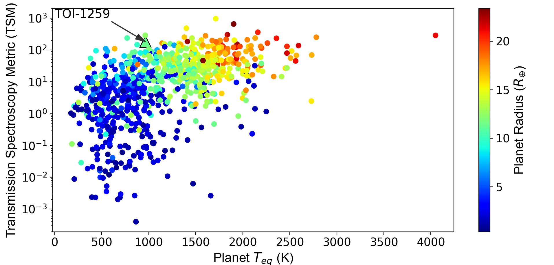
Figure 12: Transit Spectroscopy Metric (TSM) from Kempton et al. (2018) for all confirmed transiting exoplanets as a function of their equilibrium temperature (where such a value has been calculated). The TSM is calculated using Eq. 3. The color scale is the planet radius. TOI-1259Ab has a TSM of 180, making it ideal for atmospheric follow-up. In particular, it has one of the highest TSM values for a planet cooler than 1000 K and of Jupiter-size or less.

Affiliations

¹Department of Astronomy, The Ohio State University, Columbus, OH 43210, USA
²Department of Astronomy and Theoretical Astrophysics Center, University of California Berkley, Berkley, CA 94720, USA
³School of Physics and Astronomy, University of Birmingham, Edgbaston, Birmingham B15 2TT, UK
⁴American Museum of National History, New York, NY 10024, USA
⁵Center for Computational Astrophysics, Flatiron Institute, New York, NY 10010, USA
⁶Department of Astronomy, University of Washington, Seattle, WA 98105, USA
⁷Bay Area Environmental Research Institute, P.O. Box 25, Moffett Field, CA, USA
⁸School of Physics, University of New South Wales, Sydney, NSW 2052, Australia
⁹Sydney Institute for Astronomy (SIfA), School of Physics, University of Sydney, NSW 2006, Australia
¹⁰Aix Marseille Univ, CNRS, CNES, LAM, Marseille, France
¹¹Department of Physics & Astronomy, Vanderbilt University, Nashville, TN 37235, USA
¹²Center for Cosmology and AstroParticle Physics, The Ohio State University, Columbus, OH 43210, USA
¹³Acton Sky Portal Private Observatory, Acton, MA, USA
¹⁴Laboratory of Astrochemical Research, Ural Federal University, Ekaterinburg, Russia, ul. Mira d. 19, Yekaterinburg, Russia, 620002
¹⁵Astronomical department, Ural Federal University, Yekaterinburg, Russia
¹⁶Private Astronomical Observatory, Ananjev, Odessa Region, 66400, Ukraine
¹⁷Department of Physics, Engineering and Astronomy, Stephen F. Austin State University, TX 75962, USA
¹⁸Oukaimeden Observatory, High Energy Physics and Astrophysics Laboratory, Cadi Ayyad University, Marrakech, Morocco
¹⁹NASA Ames Research Center, MS 244-30, Moffett Field, CA 94035, USA
²⁰SETI Institute, 189 Bernardo Ave, Suite 200, Mountain View, CA 94043, USA
²¹Harvard-Smithsonian Center for Astrophysics, 60 Garden St, Cambridge, MA, 02138, USA
²²Department of Physics and Kavli Institute for Astrophysics and Space Research, Massachusetts Institute of Technology, Cambridge, MA 02139, USA
²³Proto-Logic LLC, 1718 Euclid Street NW, Washington, DC 20009, USA
²⁴Space Telescope Science Institute, 3700 San Martin Drive, Baltimore, MD, 21218, USA
²⁵Department of Earth, Atmospheric and Planetary Sciences, Massachusetts Institute of Technology, Cambridge, MA 02139, USA
²⁶Department of Aeronautics and Astronautics, Massachusetts Institute of Technology, Cambridge, MA 02139, USA
²⁷Department of Astronomy, The University of Wisconsin-Madison, Madison, WI 53706, USA
²⁸Department of Astrophysical Sciences, 4 Ivy Lane, Princeton University, Princeton, NJ 08544, USA
²⁹Astrophysics Group, Keele University, Keele, Staffordshire, ST5 5BG, UK ³⁰Centre for Exoplanets and Habitability, University of Warwick, Gibbet Hill Road, Coventry CV4 7AL, UK

Data availability

All TESS data are publicaly available and can be downloaded using lightkurve (Lightkurve Collaboration et al., 2018) or other tools. The SOPHIE RVs are published as supplementary data. Any other data/models in this article will be shared on reasonable request to the corresponding author.

Appendix A Nuisance parameters from the global analysis

Table 6: Fitted Gaussian process (GP) and radial velocity nuisance parameters from the joint modelling of the photometric and radial velocity data. Only the parameters for the circular orbital model are given, as the differences from the eccentric model are negligible.

Parameter	Description	Value	Prior
Sector 14
$\log{S_{0}\omega_{0}^{4}}$	GP amplitude	$-15.77^{+0.59}_{-0.51}$	$\mathcal{N}(\log{\mathrm{var(flux)}},5^{2})$
$\log{\omega_{0}}$ (${\mathrm{s}}^{-1}$)	GP frequency	$-0.90^{+0.56}_{-1.20}$	$\mathcal{N}(\log{2\pi/5},5^{2})$
$\log{\sigma^{2}}$	White noise term	$-24.52^{+3.16}_{-5.73}$	$\mathcal{N}(\log{\mathrm{var(flux)}},10^{2})$
$\mathcal{F}$	Flux scaling factor	$0.99949^{+0.00053}_{-0.00446}$	$\mathcal{N}(\mathrm{median(flux)},5^{2})$
Sector 17
$\log{S_{0}\omega_{0}^{4}}$	GP amplitude	$-8.71^{+0.28}_{-0.27}$	$\mathcal{N}(\log{\mathrm{var(flux)}},5^{2})$
$\log{\omega_{0}}$ (${\mathrm{s}}^{-1}$)	GP frequency	$0.28^{+0.32}_{-0.38}$	$\mathcal{N}(\log{2\pi/5},5^{2})$
$\log{\sigma^{2}}$	White noise term	$-24.52^{+3.29}_{-5.28}$	$\mathcal{N}(\log{\mathrm{var(flux)}},10^{2})$
$\mathcal{F}$	Flux scaling factor	$1.00051^{+0.00206}_{-0.00247}$	$\mathcal{N}(\mathrm{median(flux)},5^{2})$
Sector 18
$\log{S_{0}\omega_{0}^{4}}$	GP amplitude	$-10.19^{+0.33}_{-0.31}$	$\mathcal{N}(\log{\mathrm{var(flux)}},5^{2})$
$\log{\omega_{0}}$ (${\mathrm{s}}^{-1}$)	GP frequency	$0.75^{+0.16}_{-0.17}$	$\mathcal{N}(\log{2\pi/5},5^{2})$
$\log{\sigma^{2}}$	White noise term	$-24.86^{+3.47}_{-6.10}$	$\mathcal{N}(\log{\mathrm{var(flux)}},10^{2})$
$\mathcal{F}$	Flux scaling factor	$0.99975^{+0.00041}_{-0.00044}$	$\mathcal{N}(\mathrm{median(flux)},5^{2})$
Sector 19
$\log{S_{0}\omega_{0}^{4}}$	GP amplitude	$-14.68^{+0.50}_{-0.52}$	$\mathcal{N}(\log{\mathrm{var(flux)}},5^{2})$
$\log{\omega_{0}}$ (${\mathrm{s}}^{-1}$)	GP frequency	$-0.01^{+0.25}_{-0.29}$	$\mathcal{N}(\log{2\pi/5},5^{2})$
$\log{\sigma^{2}}$	White noise term	$-24.74^{+3.25}_{-5.49}$	$\mathcal{N}(\log{\mathrm{var(flux)}},10^{2})$
$\mathcal{F}$	Flux scaling factor	$1.00004^{+0.00019}_{-0.00019}$	$\mathcal{N}(\mathrm{median(flux)},5^{2})$
Sector 20
$\log{S_{0}\omega_{0}^{4}}$	GP amplitude	$-14.21^{+0.39}_{-0.37}$	$\mathcal{N}(\log{\mathrm{var(flux)}},5^{2})$
$\log{\omega_{0}}$ (${\mathrm{s}}^{-1}$)	GP frequency	$-0.37^{+0.24}_{-0.35}$	$\mathcal{N}(\log{2\pi/5},5^{2})$
$\log{\sigma^{2}}$	White noise term	$-24.89^{+3.19}_{-5.37}$	$\mathcal{N}(\log{\mathrm{var(flux)}},10^{2})$
$\mathcal{F}$	Flux scaling factor	$0.99995^{+0.00044}_{-0.00061}$	$\mathcal{N}(\mathrm{median(flux)},5^{2})$
Sector 21
$\log{S_{0}\omega_{0}^{4}}$	GP amplitude	$-11.36^{+0.38}_{-0.40}$	$\mathcal{N}(\log{\mathrm{var(flux)}},5^{2})$
$\log{\omega_{0}}$ (${\mathrm{s}}^{-1}$)	GP frequency	$1.04^{+0.15}_{-0.16}$	$\mathcal{N}(\log{2\pi/5},5^{2})$
$\log{\sigma^{2}}$	White noise term	$-24.77^{+3.13}_{-5.82}$	$\mathcal{N}(\log{\mathrm{var(flux)}},10^{2})$
$\mathcal{F}$	Flux scaling factor	$1.00006^{+0.00012}_{-0.00013}$	$\mathcal{N}(\mathrm{median(flux)},5^{2})$
Sector 24
$\log{S_{0}\omega_{0}^{4}}$	GP amplitude	$-11.28^{+0.42}_{-0.44}$	$\mathcal{N}(\log{\mathrm{var(flux)}},5^{2})$
$\log{\omega_{0}}$ (${\mathrm{s}}^{-1}$)	GP frequency	$1.14^{+0.16}_{-0.17}$	$\mathcal{N}(\log{2\pi/5},5^{2})$
$\log{\sigma^{2}}$	White noise term	$-24.71^{+3.26}_{-5.39}$	$\mathcal{N}(\log{\mathrm{var(flux)}},10^{2})$
$\mathcal{F}$	Flux scaling factor	$1.00007^{+0.00010}_{-0.00011}$	$\mathcal{N}(\mathrm{median(flux)},5^{2})$
Sector 25
$\log{S_{0}\omega_{0}^{4}}$	GP amplitude	$-9.83^{+0.34}_{-0.32}$	$\mathcal{N}(\log{\mathrm{var(flux)}},5^{2})$
$\log{\omega_{0}}$ (${\mathrm{s}}^{-1}$)	GP frequency	$1.51^{+0.13}_{-0.13}$	$\mathcal{N}(\log{2\pi/5},5^{2})$
$\log{\sigma^{2}}$	White noise term	$-24.64^{+3.34}_{-5.93}$	$\mathcal{N}(\log{\mathrm{var(flux)}},10^{2})$
$\mathcal{F}$	Flux scaling factor	$1.00006^{+0.00010}_{-0.00010}$	$\mathcal{N}(\mathrm{median(flux)},5^{2})$
Sector 26
$\log{S_{0}\omega_{0}^{4}}$	GP amplitude	$-13.37^{+0.63}_{-0.61}$	$\mathcal{N}(\log{\mathrm{var(flux)}},5^{2})$
$\log{\omega_{0}}$ (${\mathrm{s}}^{-1}$)	GP frequency	$0.44^{+0.24}_{-0.28}$	$\mathcal{N}(\log{2\pi/5},5^{2})$
$\log{\sigma^{2}}$	White noise term	$-24.67^{+3.33}_{-5.35}$	$\mathcal{N}(\log{\mathrm{var(flux)}},10^{2})$
$\mathcal{F}$	Flux scaling factor	$1.00005^{+0.00015}_{-0.00015}$	$\mathcal{N}(\mathrm{median(flux)},5^{2})$

Table 7: continued

Parameter	Description	Value	Prior
$R$ band
$\log{S_{0}\omega_{0}^{4}}$	GP amplitude	$2.87^{+1.82}_{-2.48}$	$\mathcal{N}(-1,10^{2})$
$\log{\omega_{0}}$ (${\mathrm{s}}^{-1}$)	GP frequency	$5.10^{+2.29}_{-0.57}$	$\mathcal{N}(\log{2\pi/0.04},10^{2})$
$\log{\sigma^{2}}$	White noise term	$-10.98^{+0.25}_{-0.29}$	$\mathcal{N}(\log{\mathrm{var(flux)}},10^{2})$
$\mathcal{F}$	Flux scaling factor	$0.89563^{+0.00080}_{-0.00069}$	$\mathcal{N}(\mathrm{median(flux)},5^{2})$
$z^{\prime}$ band
$\log{S_{0}\omega_{0}^{4}}$	GP amplitude	$-8.89^{+8.50}_{-3.46}$	$\mathcal{N}(-1,10^{2})$
$\log{\omega_{0}}$ (${\mathrm{s}}^{-1}$)	GP frequency	$2.34^{+10.24}_{-2.53}$	$\mathcal{N}(\log{2\pi/0.04},10^{2})$
$\log{\sigma^{2}}$	White noise term	$-18.14^{+4.86}_{-7.64}$	$\mathcal{N}(\log{\mathrm{var(flux)}},10^{2})$
$\mathcal{F}$	Flux scaling factor	$0.14724^{+0.00132}_{-0.00026}$	$\mathcal{N}(\mathrm{median(flux)},5^{2})$
$g^{\prime}$ band
$\log{S_{0}\omega_{0}^{4}}$	GP amplitude	$-3.14^{+1.27}_{-1.23}$	$\mathcal{N}(-1,10^{2})$
$\log{\omega_{0}}$ (${\mathrm{s}}^{-1}$)	GP frequency	$2.84^{+0.93}_{-1.20}$	$\mathcal{N}(\log{2\pi/0.04},10^{2})$
$\log{\sigma^{2}}$	White noise term	$-19.04^{+4.66}_{-7.50}$	$\mathcal{N}(\log{\mathrm{var(flux)}},10^{2})$
$\mathcal{F}$	Flux scaling factor	$0.16291^{+0.00197}_{-0.00266}$	$\mathcal{N}(\mathrm{median(flux)},5^{2})$
White light
$\log{S_{0}\omega_{0}^{4}}$	GP amplitude	$3.10^{+1.11}_{-1.03}$	$\mathcal{N}(-1,10^{2})$
$\log{\omega_{0}}$ (${\mathrm{s}}^{-1}$)	GP frequency	$3.97^{+0.42}_{-0.48}$	$\mathcal{N}(\log{2\pi/0.04},10^{2})$
$\log{\sigma^{2}}$	White noise term	$-10.90^{+0.21}_{-0.21}$	$\mathcal{N}(\log{\mathrm{var(flux)}},10^{2})$
$\mathcal{F}$	Flux scaling factor	$1.36259^{+0.00500}_{-0.00481}$	$\mathcal{N}(\mathrm{median(flux)},5^{2})$
SOPHIE
$\log{\sigma}$ ($\mathrm{km}\text{\,}{\mathrm{s}}^{-1}$)	White noise term	$-5.44^{+1.34}_{-4.40}$	$\mathcal{N}(\log{\mathrm{median(RV)}},5^{2})$
$\gamma$ ($\mathrm{km}\text{\,}{\mathrm{s}}^{-1}$)	Systemic velocity	$-40.8197^{+0.0046}_{-0.0047}$	$\mathcal{N}(\mathrm{median(RV)},0.5^{2})$

References

- Agol et al. (2020) Agol E., Luger R., Foreman-Mackey D., 2020, AJ, 159, 123
- Alexander & Lourens (1969) Alexander Lourens 1969, MNASSA, 28, 95
- Alonso et al. (2021) Alonso R., et al., 2021, arXiv e-prints, p. arXiv:2103.15720
- Althaus & Benvenuto (1998) Althaus L. G., Benvenuto O. G., 1998, MNRAS, 296, 206
- Anderson et al. (2014) Anderson D. R., et al., 2014, MNRAS, 445, 1114
- Anderson et al. (2017) Anderson D. R., et al., 2017, A&A, 604, A110
- Angus et al. (2016) Angus R., Foreman-Mackey D., Johnson J. A., 2016, ApJ, 818, 109
- Angus et al. (2019) Angus R., et al., 2019, AJ, 158, 173
- Angus et al. (2020) Angus R., et al., 2020, AJ, 160, 90
- Astropy Collaboration et al. (2013) Astropy Collaboration et al., 2013, A&A, 558, A33
- Astropy Collaboration et al. (2018) Astropy Collaboration et al., 2018, AJ, 156, 123
- Barker & Ogilvie (2009) Barker A. J., Ogilvie G. I., 2009, Monthly Notices of the Royal Astronomical Society, 395, 2268
- Barnes (2003) Barnes S. A., 2003, The Astrophysical Journal, 586, 464–479
- Bear & Soker (2014) Bear E., Soker N., 2014, Monthly Notices of the Royal Astronomical Society, 444, 1698–1704
- Bergeron et al. (1995) Bergeron P., Wesemael F., Beauchamp A., 1995, PASP, 107, 1047
- Bonsor & Veras (2015) Bonsor A., Veras D., 2015, MNRAS, 454, 53
- Bouchy et al. (2009) Bouchy F., et al., 2009, A&A, 505, 853
- Bressan et al. (2012) Bressan A., Marigo P., Girardi L., Salasnich B., Dal Cero C., Rubele S., Nanni A., 2012, MNRAS, 427, 127
- Butler et al. (2001) Butler R. P., Tinney C. G., Marcy G. W., Jones H. R. A., Penny A. J., Apps K., 2001, ApJ, 555, 410
- Butler et al. (2006) Butler R. P., et al., 2006, ApJ, 646, 505
- Chauvin, G. et al. (2006) Chauvin, G. Lagrange, A.-M. Udry, S. Fusco, T. Galland, F. Naef, D. Beuzit, J.-L. Mayor, M. 2006, A&A, 456, 1165
- Cheetham et al. (2015) Cheetham A. C., Kraus A. L., Ireland M. J., Cieza L., Rizzuto A. C., Tuthill P. G., 2015, ApJ, 813, 83
- Choi et al. (2016) Choi J., Dotter A., Conroy C., Cantiello M., Paxton B., Johnson B. D., 2016, ApJ, 823, 102
- Claret & Bloemen (2011) Claret A., Bloemen S., 2011, Astronomy and Astrophysics, 529, A75
- Curtis et al. (2019) Curtis J. L., Agüeros M. A., Douglas S. T., Meibom S., 2019, ApJ, 879, 49
- Daemgen et al. (2015) Daemgen S., Bonavita M., Jayawardhana R., Lafrenière D., Janson M., 2015, ApJ, 799, 155
- Dawson & Johnson (2018) Dawson R. I., Johnson J. A., 2018, Annual Review of Astronomy and Astrophysics, 56, 175–221
- De Gennaro et al. (2008) De Gennaro S., von Hippel T., Winget D. E., Kepler S. O., Nitta A., Koester D., Althaus L., 2008, AJ, 135, 1
- Debes et al. (2012) Debes J. H., Walsh K. J., Stark C., 2012, ApJ, 747, 148
- Desidera et al. (2014) Desidera S., et al., 2014, A&A, 567, L6
- Dotter (2016) Dotter A., 2016, ApJS, 222, 8
- Duquennoy & Mayor (1991) Duquennoy A., Mayor M., 1991, A&A, 500, 337
- Dvorak (1984) Dvorak R., 1984, Celestial Mechanics, 34, 369
- Eastman et al. (2013) Eastman J., Gaudi B. S., Agol E., 2013, Publications of the Astronomical Society of the Pacific, 125, 83
- Eastman et al. (2019) Eastman J. D., et al., 2019, arXiv e-prints, p. arXiv:1907.09480
- Eggleton & Kisseleva-Eggleton (2006) Eggleton P. P., Kisseleva-Eggleton L., 2006, Ap&SS, 304, 75
- El-Badry & Rix (2018) El-Badry K., Rix H.-W., 2018, MNRAS, 480, 4884
- El-Badry et al. (2018) El-Badry K., Rix H.-W., Weisz D. R., 2018, ApJ, 860, L17
- El-Badry et al. (2019) El-Badry K., Rix H.-W., Tian H., Duchêne G., Moe M., 2019, MNRAS, 489, 5822
- Els et al. (2001) Els S. G., Sterzik M. F., Marchis F., Pantin E., Endl M., Kürster M., 2001, A&A, 370, L1
- Fabrycky & Tremaine (2007) Fabrycky D., Tremaine S., 2007, ApJ, 669, 1298
- Faedi et al. (2010) Faedi F., West R. G., Burleigh M. R., Goad M. R., Hebb L., 2010, Monthly Notices of the Royal Astronomical Society, 410, 899–911
- Farihi (2016) Farihi J., 2016, New Astronomy Reviews, 71, 9–34
- Farmer & Agol (2003) Farmer A. J., Agol E., 2003, The Astrophysical Journal, 592, 1151
- Foreman-Mackey (2018) Foreman-Mackey D., 2018, Research Notes of the American Astronomical Society, 2, 31
- Foreman-Mackey et al. (2017) Foreman-Mackey D., Agol E., Ambikasaran S., Angus R., 2017, AJ, 154, 220
- Foreman-Mackey et al. (2020) Foreman-Mackey D., Luger R., Czekala I., Agol E., Price-Whelan A., Brandt T. D., Barclay T., Bouma L., 2020, exoplanet-dev/exoplanet v0.4.0, doi:10.5281/zenodo.1998447, https://doi.org/10.5281/zenodo.1998447
- Gänsicke et al. (2019) Gänsicke B. T., Schreiber M. R., Toloza O., Gentile Fusillo N. P., Koester D., Manser C. J., 2019, Nature, 576, 61
- Green et al. (2019) Green G. M., Schlafly E., Zucker C., Speagle J. S., Finkbeiner D., 2019, ApJ, 887, 93
- Guidry et al. (2020) Guidry J. A., et al., 2020, I Spy Transits and Pulsations: Empirical Variability in White Dwarfs Using Gaia and the Zwicky Transient Facility (arXiv:2012.00035)
- Hamers et al. (2016) Hamers A. S., Perets H. B., Portegies Zwart S. F., 2016, MNRAS, 455, 3180
- Hartman & Lépine (2020) Hartman Z. D., Lépine S., 2020, ApJS, 247, 66
- Hayden et al. (2015) Hayden M. R., et al., 2015, ApJ, 808, 132
- Hedges et al. (2020) Hedges C., Angus R., Barentsen G., Saunders N., Montet B. T., Gully-Santiago M., 2020, Research Notes of the AAS, 4, 220
- Hellier et al. (2014) Hellier C., et al., 2014, MNRAS, 440, 1982
- Holberg & Bergeron (2006) Holberg J. B., Bergeron P., 2006, AJ, 132, 1221
- Holman & Wiegert (1999) Holman M. J., Wiegert P. A., 1999, AJ, 117, 621
- Husser et al. (2013) Husser T.-O., Wende-von Berg S., Dreizler S., Homeier D., Reiners A., Barman T., Hauschildt P. H., 2013, Astronomy and Astrophysics, 553, A6
- Jenkins et al. (2016) Jenkins J. M., et al., 2016, in Software and Cyberinfrastructure for Astronomy IV. p. 99133E, doi:10.1117/12.2233418
- Jeong et al. (2018) Jeong G., Han I., Park M.-G., Hatzes A. P., Bang T.-Y., Gu S., Bai J., Lee B.-C., 2018, AJ, 156, 64
- Jørgensen, B. R. & Lindegren, L. (2005) Jørgensen, B. R. Lindegren, L. 2005, A&A, 436, 127
- Kempton et al. (2018) Kempton E. M.-R., et al., 2018, Publications of the Astronomical Society of the Pacific, 130, 114401
- Kozai (1962) Kozai Y., 1962, AJ, 67, 591
- Kratter & Perets (2012) Kratter K. M., Perets H. B., 2012, ApJ, 753, 91
- Kraus et al. (2012) Kraus A. L., Ireland M. J., Hillenbrand L. A., Martinache F., 2012, ApJ, 745, 19
- Kraus et al. (2016) Kraus A. L., Ireland M. J., Huber D., Mann A. W., Dupuy T. J., 2016, AJ, 152, 8
- Kreidberg et al. (2018) Kreidberg L., Line M. R., Thorngren D., Morley C. V., Stevenson K. B., 2018, ApJ, 858, L6
- Kurucz (1979) Kurucz R. L., 1979, ApJS, 40, 1
- Lagrange et al. (2006) Lagrange Beust Udry, Chauvin. Mayor 2006, A&A, 459, 955
- Lépine & Bongiorno (2007) Lépine S., Bongiorno B., 2007, AJ, 133, 889
- Lidov (1962) Lidov M. L., 1962, Planet. Space Sci., 9, 719
- Lightkurve Collaboration et al. (2018) Lightkurve Collaboration et al., 2018, Lightkurve: Kepler and TESS time series analysis in Python, Astrophysics Source Code Library (ascl:1812.013)
- Louie et al. (2018) Louie D. R., Deming D., Albert L., Bouma L. G., Bean J., Lopez-Morales M., 2018, PASP, 130, 044401
- Luger et al. (2019) Luger R., Agol E., Foreman-Mackey D., Fleming D. P., Lustig-Yaeger J., Deitrick R., 2019, The Astronomical Journal, 157, 64
- Manser et al. (2019) Manser C. J., et al., 2019, Science, 364, 66
- Mardling & Aarseth (2001) Mardling R. A., Aarseth S. J., 2001, MNRAS, 321, 398
- Maxted et al. (2000) Maxted P. F. L., Marsh T. R., Moran C. K. J., 2000, Monthly Notices of the Royal Astronomical Society, 319, 305
- Mayor et al. (2004) Mayor Udry Naef Pepe Queloz Santos Burnet 2004, A&A, 415, 391
- Mazeh & Shaham (1979) Mazeh T., Shaham J., 1979, A&A, 77, 145
- Moe & Kratter (2019) Moe M., Kratter K. M., 2019, arXiv e-prints, p. arXiv:1912.01699
- Montgomery et al. (1999) Montgomery M. H., Klumpe E. W., Winget D. E., Wood M. A., 1999, ApJ, 525, 482
- Morton et al. (2016) Morton T. D., Bryson S. T., Coughlin J. L., Rowe J. F., Ravichandran G., Petigura E. A., Haas M. R., Batalha N. M., 2016, ApJ, 822, 86
- Mugrauer (2019) Mugrauer M., 2019, Monthly Notices of the Royal Astronomical Society, 490, 5088
- Mugrauer & Dinçel (2016) Mugrauer M., Dinçel B., 2016, Astronomische Nachrichten, 337, 627
- Mugrauer & Michel (2020) Mugrauer M., Michel K. U., 2020, Gaia Search for stellar Companions of TESS Objects of Interest (arXiv:2009.12234)
- Mugrauer, M. et al. (2007) Mugrauer, M. Neuhäuser, R. Mazeh, T. 2007, A&A, 469, 755
- Naef et al. (2010) Naef et al., 2010, A&A, 523, A15
- Naoz (2016) Naoz S., 2016, Annual Review of Astronomy and Astrophysics, 54, 441–489
- Naoz et al. (2012) Naoz S., Farr W. M., Rasie F. A., 2012, ApJ, 754, L36
- Neveu-VanMalle et al. (2014) Neveu-VanMalle M., et al., 2014, A&A, 572, A49
- Nortmann et al. (2018) Nortmann L., et al., 2018, Science, 362, 1388
- Parviainen & Aigrain (2015) Parviainen H., Aigrain S., 2015, Monthly Notices of the Royal Astronomical Society, 453, 3821
- Perruchot et al. (2008) Perruchot S., et al., 2008, in Ground-based and Airborne Instrumentation for Astronomy II. p. 70140J, doi:10.1117/12.787379
- Qian et al. (2009) Qian S. B., Dai Z. B., Liao W. P., Zhu L. Y., Liu L., Zhao E. G., 2009, ApJ, 706, L96
- Queloz et al. (2000) Queloz D., et al., 2000, A&A, 354, 99
- Reid (1996) Reid I. N., 1996, AJ, 111, 2000
- Salvatier et al. (2016) Salvatier J., Wiecki T. V., Fonnesbeck C., 2016, PeerJ Computer Science, 2, e55
- Schlegel et al. (1998) Schlegel D. J., Finkbeiner D. P., Davis M., 1998, ApJ, 500, 525
- Ségransan et al. (2010) Ségransan D., et al., 2010, A&A, 511, A45
- Shappee & Thompson (2013) Shappee B. J., Thompson T. A., 2013, ApJ, 766, 64
- Silvotti et al. (2014) Silvotti R., Sozzetti A., Lattanzi M., Morbidelli R., 2014, Detectability of substellar companions around white dwarfs with Gaia (arXiv:1412.3307)
- Smith et al. (2012) Smith J. C., et al., 2012, PASP, 124, 1000
- Southworth et al. (2020) Southworth J., Tremblay P.-E., Gänsicke B. T., Evans D., Močnik T., 2020, MNRAS, 497, 4416
- Spada & Lanzafame (2020) Spada F., Lanzafame A. C., 2020, A&A, 636, A76
- Spake et al. (2018) Spake J. J., et al., 2018, Nature, 557, 68
- Stassun & Torres (2016) Stassun K. G., Torres G., 2016, AJ, 152, 180
- Stassun & Torres (2018) Stassun K. G., Torres G., 2018, ApJ, 862, 61
- Stassun et al. (2017) Stassun K. G., Collins K. A., Gaudi B. S., 2017, AJ, 153, 136
- Stassun et al. (2018) Stassun K. G., Corsaro E., Pepper J. A., Gaudi B. S., 2018, AJ, 155, 22
- Stein et al. (2013) Stein N. M., van Dyk D. A., von Hippel T., DeGennaro S., Jeffery E. J., Jefferys W. H., 2013, Statistical Analysis and Data Mining: The ASA Data Science Journal, 9, 34
- Stenning et al. (2016) Stenning D. C., Wagner-Kaiser R., Robinson E., van Dyk D. A., von Hippel T., Sarajedini A., Stein N., 2016, ApJ, 826, 41
- Stephan et al. (2017) Stephan A. P., Naoz S., Zuckerman B., 2017, ApJ, 844, L16
- Stephan et al. (2018) Stephan A. P., Naoz S., Gaudi B. S., 2018, AJ, 156, 128
- Stephan et al. (2020a) Stephan A. P., Naoz S., Gaudi B. S., 2020a, Giant Planets, Tiny Stars: Producing Short-Period Planets around White Dwarfs with the Eccentric Kozai-Lidov Mechanism (arXiv:2010.10534)
- Stephan et al. (2020b) Stephan A. P., Naoz S., Gaudi B. S., Salas J. M., 2020b, ApJ, 889, 45
- Stumpe et al. (2012) Stumpe M. C., et al., 2012, PASP, 124, 985
- Stumpe et al. (2014) Stumpe M. C., Smith J. C., Catanzarite J. H., Van Cleve J. E., Jenkins J. M., Twicken J. D., Girouard F. R., 2014, PASP, 126, 100
- Theano Development Team (2016) Theano Development Team 2016, arXiv e-prints, abs/1605.02688
- Thébault et al. (2008) Thébault P., Marzari F., Scholl H., 2008, Monthly Notices of the Royal Astronomical Society, 388, 1528–1536
- Tian et al. (2020) Tian H.-J., El-Badry K., Rix H.-W., Gould A., 2020, ApJS, 246, 4
- Tokovinin (2014) Tokovinin A., 2014, AJ, 147, 87
- Torres et al. (2010) Torres G., Andersen J., Giménez A., 2010, A&ARv, 18, 67
- Vanderbosch et al. (2020) Vanderbosch Z., et al., 2020, ApJ, 897, 171
- Vanderburg et al. (2015a) Vanderburg A., et al., 2015a, Nature, 526, 546–549
- Vanderburg et al. (2015b) Vanderburg A., et al., 2015b, ApJ, 800, 59
- Vanderburg et al. (2020) Vanderburg A., et al., 2020, Nature, 585, 363–367
- Veras et al. (2011) Veras D., Wyatt M. C., Mustill A. J., Bonsor A., Eldridge J. J., 2011, Monthly Notices of the Royal Astronomical Society, 417, 2104–2123
- Veras et al. (2013) Veras D., Mustill A. J., Bonsor A., Wyatt M. C., 2013, MNRAS, 431, 1686
- Wang et al. (2014) Wang J., Fischer D. A., Xie J.-W., Ciardi D. R., 2014, ApJ, 791, 111
- Williams et al. (2009) Williams K. A., Bolte M., Koester D., 2009, ApJ, 693, 355
- Wilson et al. (2019) Wilson T. G., Farihi J., Gänsicke B. T., Swan A., 2019, MNRAS, 487, 133
- Wittenmyer et al. (2013) Wittenmyer R. A., Horner J., Marshall J. P., 2013, Monthly Notices of the Royal Astronomical Society, 431, 2150–2154
- Xie et al. (2009) Xie J.-W., Zhou J.-L., Ge J., 2009, The Astrophysical Journal, 708, 1566
- Ziegler et al. (2021) Ziegler C., Tokovinin A., Latiolais M., Briceno C., Law N., Mann A. W., 2021, arXiv e-prints, p. arXiv:2103.12076
- Zorotovic & Schreiber (2013) Zorotovic M., Schreiber M. R., 2013, A&A, 549, A95
- von Hippel et al. (2006) von Hippel T., Jefferys W. H., Scott J., Stein N., Winget D. E., De Gennaro S., Dam A., Jeffery E., 2006, ApJ, 645, 1436