Model reduction techniques for the computation of extended Markov parameterizations for generalized Langevin equations

Abstract

The generalized Langevin equation is a model for the motion of coarse-grained particles where dissipative forces are represented by a memory term. The numerical realization of such a model requires the implementation of a stochastic delay-differential equation and the estimation of a corresponding memory kernel. Here we develop a new approach for computing a data-driven Markov model for the motion of the particles, given equidistant samples of their velocity autocorrelation function. Our method bypasses the determination of the underlying memory kernel by representing it via up to about twenty auxiliary variables. The algorithm is based on a sophisticated variant of the Prony method for exponential interpolation and employs the Positive Real Lemma from model reduction theory to extract the associated Markov model. We demonstrate the potential of this approach for the test case of anomalous diffusion, where data are given analytically, and then apply our method to velocity autocorrelation data of molecular dynamics simulations of a colloid in a Lennard-Jones fluid. In both cases, the VACF and the memory kernel can be reproduced very accurately. Moreover, we show that the algorithm can also handle input data with large statistical noise. We anticipate that it will be a very useful tool in future studies that involve dynamic coarse-graining of complex soft matter systems.

Keywords: coarse-graining, model reduction, exponential interpolation, Prony’s method, Positive Real Lemma, nonsymmetric Lanczos method

1 Introduction

Generalized Langevin Equations (GLE)s, i.e., extensions of Langevin equations with memory, have fascinated scientists for many decades, ever since they were first introduced by Mori in the 60s [40] based on concepts of Zwanzig [52]. Their purpose is to describe in very general terms the irreversible dynamics of collective (coarse-grained) observables in many-particle systems without having to assume complete separation of time scales. Consider a multiparticle system at thermal equilibrium, and assume we are interested in the dynamical evolution of a given set $\mathbf{A}(t)$ of coarse-grained variables. For such cases, starting from a microscopic Hamiltonian description and using a projection operator formalism, Mori and Zwanzig derived a dynamical equation of the following form for $\mathbf{A}(t)$ [53]

$$\dot{\mathbf{A}}(t)=\mathbf{F}^{C}(\mathbf{A}(t))-\int_{0}^{t}{\rm d}s\,\mathbf{K}(t-s)\mathbf{A}(s)+\mathbf{F}^{R}(t).$$ (1)

Here $\mathbf{F}^{C}(\mathbf{A}(t))=\textrm{i}\Omega\mathbf{A}$ describes the collective oscillations of $\mathbf{A}(t)$, $\mathbf{K}(t)$ a memory kernel matrix, and $\mathbf{F}^{R}(t)$ incorporates nonlinear terms and interactions with the remaining microscopic degrees of freedom and is interpreted as a stochastic process. It is connected to the memory kernel via a fluctuation-dissipation relation

$$\langle\mathbf{F}^{R}(t)\mathbf{F}^{R}(t^{\prime})\rangle=\mathbf{K}(t-t^{\prime})\langle\mathbf{A}\mathbf{A}\rangle,$$ (2)

where $\mathbf{F}^{R}(t)\mathbf{F}^{R}(t^{\prime})$ and $\mathbf{A}\mathbf{A}$ denote tensor products and $\langle\cdot\rangle$ configurational averages. In the limit where the memory kernel decays almost instantaneously, Eq. (1) can be replaced by a standard Markovian Langevin equation with friction $\mathbf{K}_{0}=\int_{0}^{\infty}\textrm{d}s\>\mathbf{K}(s)$ and uncorrelated noise $\mathbf{F}^{R}(t)$ satisfying $\langle\mathbf{F}^{R}(t)\mathbf{F}^{R}(t^{\prime})\rangle=2\mathbf{K}_{0}\delta(t-t^{\prime})\langle\mathbf{A}\mathbf{A}\rangle$.

Eq. (1) can be generalized to stationary and even non-stationary nonequilibrium systems [22, 39]. Using modified projector methods, it is possible to design GLEs such that $\mathbf{F}^{C}$ includes all (linear and nonlinear) reversible interactions [29], and the memory and noise terms subsume the remaining dissipative contributions to the dynamical equations. In that case, the latter can also be seen as a frequency dependent thermostat [53]. Independent of the original dynamic coarse-graining context, such GLE thermostats have been utilized to devise enhanced sampling approaches in molecular dynamics simulations [9] and even as means to mimic the effect of nuclear quantum fluctuations [10]. From a more fundamental point of view, GLEs are popular theoretical frameworks to describe intriguing physical phenomena such as anomalous diffusion [38, 26, 21] or the glass transition [20].

In numerical simulations of GLEs, one faces two main challenges: First, the efficient evaluation of the history dependent memory term, and second, the generation of suitably correlated random numbers for the stochastic term. If the memory kernel has a finite range, a straightforward direct integration of the GLE is possible [14, 46, 12, 33, 27, 28]. However, depending on the memory range, the integration can be time consuming, and the necessity to impose a sharp cutoff may cause problems. Therefore, already early on, alternative approaches have been explored where the GLE is approximated by an extended Markovian system, either using autoregressive techniques [41, 13, 17, 37] or by introducing additional, auxiliary degrees of freedom [11, 5, 47, 35]. In both cases, the memory kernel is effectively approximated by a sum of exponentials. Integrating GLEs via extended Markovian schemes has several advantages over direct integration. First, the hard cutoff of the memory kernel is replaced by a less severe exponential cutoff. Second, the integration is often faster [33]. Third, the integration scheme can be implemented in a straightforward manner using established algorithms for Langevin equations.

To simplify the discussion, in the following, we will focus on GLEs that describe the Brownian motion of selected tagged particles (e.g., colloids or polymers) in a bath of surrounding particles. The coarse-grain quantity of interest is the velocity $V(t)$ of the center of mass of the tagged particle. Our considerations and methods can easily be generalized to other GLEs as well. The derivation of extended Markov systems for approximating the solution of such GLEs has been treated in several papers. The standard work flow consists of three steps. In a first step an approximation of the memory kernel is determined. In some cases, this is done directly by using the Mori-Zwanzig formalism analytically [12, 36], or by analyzing trajectories in microscopic simulations with concepts from the Mori-Zwanzig theory [8]. More often, one uses known velocity and force correlation functions from all-atom simulations [27, 28, 32, 33, 51] as input data and solves a first kind or second kind Volterra integral equation. Care has to be taken in this latter case, because first kind integral equations are notoriously ill-conditioned [7, 31, 45]. In a second step the computed memory kernel is approximated by an exponential series, known as a Prony series; this can be achieved by using rational approximations of the Laplace transform of the memory kernel, or by some general nonlinear fitting scheme [5, 19, 32, 36]; both methods, however, are only feasible for few terms of this exponential series. Finally, the coefficients of the extended Langevin model can be extracted from the coefficients of the exponential approximation [11, 19, 42].

In case the starting point is the velocity autocorrelation function (VACF), determining the memory kernel prior to expanding it seems an unecessary detour. It should be more efficient and less error-prone to extract and optimize the parameters of the integrator directly from the VACF data. Wang et al. have taken this direct route and determined the parameters of a Prony series with up to eight terms by training a deep neural network in two steps with VACF data [49]. Using the example of dilute and dense star polymer solutions, they showed that their GLE integrator is able to reproduce the early and late time characteristics of the VACF over several orders of magnitude in time. This example demonstrates the potential of direct optimization. However, their machine learning based method requires a complicated training procedure involving a series of GLE simulations, similar to other iterative memory reconstruction methods [27]. Therefore, it gives little insight into the mathematical structure of the problem, and in particular, the impact of noise in the input data remains unclear.

In the present paper, we propose an analytical method to directly determine the Langevin model from a finite number of samples of the VACF. We avoid taking the detour of computing an intermediate memory kernel and thus circumvent a significant cause of numerical errors. Our approach adapts techniques which have originally been developed for the purpose of model reduction in deterministic dynamical systems [15, 18]. Some of these have already been used in the context of stochastic dynamical systems [6, 16], but here we follow a different route.

The paper is organized as follows. In Section 2, we describe the background and major ideas behind our model reduction algorithm; more technical details have been shifted into three appendices at the end of this text. Then, in Section 3, we discuss numerical results for three different case studies: one setting uses analytic data (“subdiffusion”), a second example treats molecular dynamics (MD) data taken from our earlier paper [27], and the final case study considers a sequence of MD data sets with different amounts of statistical noise. A final discussion of our results in Section 4 concludes this work.

2 Methods

In this paper we restrict ourselves to a one-dimensional system, and postpone the nontrivial technical generalization to higher dimensional problems to future work. We thus consider specifically the GLE

$$\ m\dot{V}(t)\,=\,-\!\int_{-\infty}^{t}{\rm d}s\,\gamma(t-s)V(s)\,+\,F^{R}(t)$$ (3)

for the scalar velocity $V$ of a macroparticle with mass $m>0$, where the memory kernel $\gamma$ is taken to be continuous and integrable. The lower bound of the integral in Eq. (3) is chosen $-\infty$ to indicate that we are considering the stationary limit of a process where the origin of time does not matter. In order to fulfill the fluctuation-dissipation theorem the random force $F^{R}$ is assumed to be a stationary Gaussian process with zero mean, satisfying

$$\ \langle F^{R}(t)F^{R}(t^{\prime})\rangle\,=\,\frac{1}{\beta}\,\gamma(t-t^{\prime})\,,$$

where $\beta$ is the inverse temperature [44]. The corresponding solution $V$ is a stationary Gaussian process with zero mean and autocorrelation function

$$\ C_{V}(t-t^{\prime})\,=\,\langle V(t)V(t^{\prime})\rangle\,.$$ (4)

We assume that samples

$$\ y_{\nu}\,=\,\beta m\,C_{V}(t_{\nu})$$ (5)

of this autocorrelation function are given on an equidistant grid

$$\ \triangle\,=\,\{t_{\nu}\,=\,\nu\tau\,:\,\nu=0,\dots,2n-1\}$$ (6)

for some $n\geq 2$ and mesh size $\tau>0$. Due to the particular specification (5) these data are normalized to satisfy $y_{0}=1$ up to statistical errors. In the initialization step of our algorithm we therefore rescale the data to exactly match this physical constraint.

Our goal is the derivation of a Langevin equation

$$\ {\rm d}\!\left[\hskip-5.0pt\begin{array}[]{*\c@MaxMatrixCols c}{\tilde{V}}\\ Z\end{array}\hskip-5.0pt\right]\,=\,k\left[\hskip-5.0pt\begin{array}[]{*\c@MaxMatrixCols c}\phantom{-}0\phantom{{}_{1}}&\!\hskip 0.43057pte_{1}^{T}\\ \!-e_{1}&\!T_{0}\end{array}\hskip-5.0pt\right]\left[\hskip-5.0pt\begin{array}[]{*\c@MaxMatrixCols c}{\tilde{V}}\\ Z\end{array}\hskip-5.0pt\right]{\rm d}t+\left[\hskip-5.0pt\begin{array}[]{*\c@MaxMatrixCols c}\,0\\ g\end{array}\hskip-5.0pt\right]{\rm d}W$$ (15)

for an approximate velocity ${\tilde{V}}$ and a set of auxiliary variables $Z\in{\mathord{\mathbb{R}}}^{N}$, with $e_{1}$ being the first canonical basis vector in ${\mathord{\mathbb{R}}}^{N}$ and $W$ a one-dimensional Brownian motion. We are interested in the stationary solution of (15), and we want to achieve ${\tilde{V}}\approx V$ by choosing the coefficients $k\in{\mathord{\mathbb{R}}}$, $g\in{\mathord{\mathbb{R}}}^{N}$, and the tridiagonal matrix $T_{0}\in{\mathord{\mathbb{R}}}^{N\times N}$ in such a way that the autocorrelation function $C_{\tilde{V}}$ of ${\tilde{V}}$ is given by a finite Prony series

$$\ C_{\tilde{V}}(t)\,=\,\frac{1}{\beta m}\sum_{j=1}^{N+1}w_{j}e^{\lambda_{j}t},\quad t\geq 0\,,$$ (16)

and interpolates the given data at the $2n$ grid points of $\triangle$, i.e.,

$$\ \beta m\,C_{\tilde{V}}(t_{\nu})\,\approx\,y_{\nu}\,,\quad\nu=0,\dots,2n-1\,.$$ (17)

We mention that if the memory kernel is of interest for diagnostic purposes then it can readily be computed as

$$\ \gamma(t)\,=\,k^{2}e_{1}^{T}e^{t\hskip 0.3014ptkT_{0}}e_{1}\,,\quad t\geq 0\,.$$ (18)

2.1 Prony’s method

In the first step of our approach we determine the solution

$$\ f(t)\,=\,\sum_{j=1}^{n}w_{j}e^{\lambda_{j}t}$$ (19)

of the exponential interpolation problem

$$\ f(t_{\nu})\,=\,y_{\nu}\,,\quad\nu=0,\dots,2n-1\,.$$ (20)

For this we use a variant of Prony’s method, which we borrow from [1]. This algorithm computes the Lanczos polynomials associated with the moment functional defined by the given data (see C for more details) and uses the corresponding recursion coefficients to set up a (real) tridiagonal Jacobi matrix $J\in{\mathord{\mathbb{R}}}^{n\times n}$. The key observation behind the algorithm is that this matrix solves the moment problem

$$\ e_{1}^{T}J^{\nu}e_{1}=y_{\nu}\,,\quad\nu=0,\dots,2n-1\,,$$ (21)

where now $e_{1}=[1,0,\dots,0]^{T}$ is the first canonical basis vector in ${\mathord{\mathbb{R}}}^{n}$.

We should mention that the interpolation problem (19), (20) need not have a solution, and that this recursive algorithm can break down, but we never encountered this problem in our experiments. We also assume in the sequel that $J$ has $n$ distinct eigenvalues $\mu_{j}$ to simplify the presentation. Then we can factorize

$$\ J\,=\,XDX^{-1}\,,$$ (22)

where $D$ is a diagonal matrix with the eigenvalues $\mu_{j}$ on its diagonal; the columns $x_{j}$ of

$$\ X\,=\,[x_{1},\dots,x_{n}]$$ (23)

are the associated eigenvectors. Given this factorization we then let

$$\ A\,=\,\frac{1}{\tau}\log J\,=\,X\Lambda X^{-1}\,,$$ (24)

where $\Lambda\in{\mathord{\mathbb{R}}}^{n\times n}$ is the diagonal matrix with the eigenvalues

$$\ \lambda_{j}\,=\,\frac{1}{\tau}\log\mu_{j}$$ (25)

of $A$ on its diagonal. It follows that $e^{\nu\tau A}=J^{\nu}$ for $\nu\in{\mathord{\mathbb{N}}}_{0}$, and hence,

$$\ f(t)\,=\,e_{1}^{T}e^{tA}e_{1}$$ (26)

is the desired solution of the interpolation problem (20).

When the memory kernel is integrable and continuous then the autocorrelation function $C_{V}$ is differentiable with

$$\ \dot{C}_{V}(0)\,=\,0\,.$$

We therefore also like to impose the condition $\dot{f}(0)=0$ for the Prony series (26), which gives

$$\ 0\,\mathop{=}\limits^{!}\,\dot{f}(0)\,=\,e_{1}^{T}Ae_{1}\,=\,A_{1,1}\,.$$ (27)

In general, however, the matrix $A$ generated in (24) does not satisfy this constraint. Our remedy for this shortcoming is that we blame this on measurement errors in $y_{1}=\beta m\,C_{V}(\tau)$, i.e., the first nontrivial data point, and we seek to perturb $y_{1}$ in such a way that (27) is satisfied. We apply a Newton iteration for this purpose, which is described in A.

We emphasize that the problem of fitting exponentials to given data is known to be highly ill-conditioned [48]. In our context this is reflected by the presence of spurious exponentials in (19) with exponents $\lambda_{j}$ in the closed right-half plane, corresponding to eigenvalues $\mu_{j}$ of $J$ in the exterior of the unit disk or on the unit circle. The corresponding exponentials are unphysical because they do not converge to zero. Fortunately, though, if $\tau$ has been properly chosen and the data noise is not too big (see Section 3 below), then the respective terms in (19) come with weights, which are by several orders of magnitude smaller than those of the relevant terms. We therefore delete the spurious terms from the series representation of $f$ defined in (26) by eliminating the corresponding eigenvalues. This modification is described in more detail in B.

Another issue that is worth mentioning concerns negative eigenvalues $\mu_{j}$ (within the unit disk) of the Jacobi matrix – in particular, because this detail is not addressed at all in [1]. The complex logarithm which is employed in (25) is defined in the complex plane except for a cut along the nonpositive real axis. However, the presence of eigenvalues $\mu_{j}\in(-1,0)$ makes sense physically; in view of (21) those correspond to damped oscillations in the data, and hence, to terms of the form

$$\ w_{j}|\mu_{j}|^{t/\tau}\!\cos(\pi t/\tau)$$ (28)

in (19). As the logarithm is multivalued for negative arguments we need to replace the corresponding formula (25) by adding two eigenvalues

$$\ \lambda_{\pm j}\,=\,\frac{1}{\tau}\log|\mu_{j}|\,\pm\,\frac{\pi}{\tau}\,\rmi$$ (29)

to the spectrum of $A$ for a correct representation of this term in (26). Again, we refer to B to illustrate how this can be achieved.

The final matrix $A$ has the form

$$\ A\,=\,\left[\hskip-5.0pt\begin{array}[]{*\c@MaxMatrixCols c}\phantom{-}0&b^{T}\\ -c&A_{0}\end{array}\hskip-5.0pt\right].$$ (32)

It is no longer $n\times n$, but typically has a smaller dimension $(N+1)\times(N+1)$, because of the elimination of the spurious eigenvalues.

2.2 The Positive Real Lemma

In a second step of our algorithm we determine a vector $\ell\in{\mathord{\mathbb{R}}}^{N}$, such that the auxiliary Langevin equation

$$\ {\rm d}\!\left[\hskip-5.0pt\begin{array}[]{*\c@MaxMatrixCols c}{\tilde{V}}\\ Y\end{array}\hskip-5.0pt\right]\,=\,\left[\hskip-5.0pt\begin{array}[]{*\c@MaxMatrixCols c}\phantom{-}0&b^{T}\\ -c&A_{0}\end{array}\hskip-5.0pt\right]\left[\hskip-5.0pt\begin{array}[]{*\c@MaxMatrixCols c}{\tilde{V}}\\ Y\end{array}\hskip-5.0pt\right]{\rm d}t+\left[\hskip-5.0pt\begin{array}[]{*\c@MaxMatrixCols c}\,0\\ \ell\end{array}\hskip-5.0pt\right]{\rm d}W$$ (41)

with the system matrix determined in (32) has a stationary solution, whose autocorrelation function $C_{\tilde{V}}$ is given by (16). Before doing so let us make two remarks.

1. Due to our construction the matrix $A$ of (32) has only eigenvalues with negative real part. Therefore, the Langevin equation (41) has a unique stationary solution, and the corresponding autocorrelation function $C_{\tilde{V}}$ is given by

   $$\ C_{\tilde{V}}(t)\,=\,\frac{1}{\beta m}\,e_{1}^{T}e^{|t|\!\hskip 0.3014ptA}\Sigma\,e_{1}\,,$$ (42)

   where the covariance matrix $\Sigma$ is the solution of the Lyapunov equation

   $$\ A\Sigma\,+\,\Sigma A^{T}\,=\,-\beta m\left[\hskip-5.0pt\begin{array}[]{*\c@MaxMatrixCols c}0&0\\ 0&\ell\ell^{T}\end{array}\hskip-5.0pt\right],$$ (43)

   cf., e.g., [42]. Since we want $\beta m\,C_{\tilde{V}}(t)$ to match the Prony series $f(t)$ for $t\geq 0$ we conclude from (42) and (26) that we need to impose the constraint

   $$\ \Sigma\,e_{1}\,=\,e_{1}\,,$$ (44)

   i.e., the covariance matrix has to satisfy

   $$\ \Sigma\,=\,\left[\hskip-5.0pt\begin{array}[]{*\c@MaxMatrixCols c}1&0\\ 0&\Sigma_{0}\end{array}\hskip-5.0pt\right]$$ (45)

   for some symmetric, positive, semidefinite matrix $\Sigma_{0}\in{\mathord{\mathbb{R}}}^{N\times N}$.

   Inserting (32) and (44) into (43), we see that (43) is equivalent to the system

   $$\eqalign{\ A_{0}\Sigma_{0}+\Sigma_{0}A_{0}^{T}\,=\,-\beta m\,\ell\ell^{T}\,,\cr\ \Sigma_{0}b\,=\,c\,,}$$ (46)

   which is known as (singular) Lur’e equations.

2. From the Lur’e equations it is evident that a necessary condition for the existence of an approximate Langevin system (41) is that all eigenvalues of $A_{0}$ must have nonpositive real part.

   Another necessary condition stems from the well-known fact that $C_{\tilde{V}}$ is per se a function of positive type, i.e., its Fourier transform $\widehat{C}_{\tilde{V}}$ is nonnegative. Since

   $$\ \widehat{C}_{\tilde{V}}(\omega)=\frac{2}{\beta m}{\rm Re}\Bigl{(}\rmi\omega+b^{T}\!(\rmi\omega I-A_{0})^{-1}c\!\Bigr{)}^{\!-1}$$

   by virtue of (42) and (32), it follows that this condition is satisfied, if and only if

   $$\ {\rm Re}\Bigl{(}b^{T}(\rmi\omega I-A_{0})^{-1}c\Bigr{)}\,\geq\,0$$ (47)

   for all $\omega\geq 0$.

   This is a familiar condition in control theory, where the function

   $$\ \kappa(s)\,=\,b^{T}(sI-A_{0})^{-1}c$$ (48)

   is known as the transfer function associated with the system (41). Because of our previous statement this function is analytic in the open right-half plane, and if it also satisfies (47) then it is called positive real. Unfortunately, it is hard to deduce from (19) whether the transfer function $\kappa$ is positive real.

We have seen that a necessary condition to find a solution of the Lur’e equations (46) is, that the transfer function $\kappa$ be positive real. On the other hand a classical result from Anderson [2] states that the Lur’e equations do indeed have a solution when $\kappa$ is positive real. Even better, there is also a constructive algorithm for computing $\Sigma_{0}$ and $\ell$; see C. Therefore the computation of the coefficients of the extended Langevin equation (41) is settled in the positive real case. When this algorithm fails, on the other hand, then this means that the transfer function (48) lacks to be positive real, and then no extended Langevin model (41) exists for this particular set of data. Usually this means that the grid spacing $\tau$ or the number $2n$ of grid points is either too big or too small (see Section 3).

2.3 A final Lanczos sweep

The system matrix $A$ of the auxiliary Langevin equation (41) is a full matrix, in general, and hence, the numerical integration of (41) amounts to $O(N^{2})$ operations per time step. We therefore perform a coordinate transformation

$$\ T\,=\,U^{-1}AU$$ (49)

such that $T$ is a tridiagonal matrix (which reduces the work load of the time integration to $O(N)$ operations per time step).

The matrix $U$ and its inverse can be determined with the (nonsymmetric) Lanczos method [30], which generates two vector sequences $u_{0},\dots,u_{N}$ and $v_{0},\dots,v_{N}$ in ${\mathord{\mathbb{R}}}^{N+1}$ with

$$\ v_{i}^{T}u_{j}\,=\,\delta_{ij}\,,\quad i,j=0,\dots,N\,.$$ (50)

When choosing $u_{0}$ and $v_{0}$ as the first canonical basis vector in ${\mathord{\mathbb{R}}}^{N+1}$ then it follows from the biorthogonality relation (50) that

$$\ U\,=\,[u_{0},\dots,u_{N}]\,=\,\left[\hskip-5.0pt\begin{array}[]{*\c@MaxMatrixCols c}1&0\\ 0&U_{0}\end{array}\hskip-5.0pt\right]$$ (51)

for some $U_{0}\in{\mathord{\mathbb{R}}}^{N\times N}$, and that

$$\ U^{-1}\,=\,\left[\hskip-5.0pt\begin{array}[]{*\c@MaxMatrixCols c}1&0\\ 0&U_{0}^{-1}\end{array}\hskip-5.0pt\right]\,=\,[v_{0},\dots,v_{N}]\,.$$

With $g=U_{0}^{-1}\ell$ and new variables $Z=U_{0}^{-1}Y$ the Langevin equation (41) is transformed into

$$\ {\rm d}\!\left[\hskip-5.0pt\begin{array}[]{*\c@MaxMatrixCols c}{\tilde{V}}\\ Z\end{array}\hskip-5.0pt\right]\,=\,\left[\hskip-5.0pt\begin{array}[]{*\c@MaxMatrixCols c}\,0&\!\!b^{T}U_{0}\\ -U_{0}^{-1}c&\!\!T_{0}^{\prime}\end{array}\hskip-5.0pt\right]\left[\hskip-5.0pt\begin{array}[]{*\c@MaxMatrixCols c}{\tilde{V}}\\ Z\end{array}\hskip-5.0pt\right]{\rm d}t+\left[\hskip-5.0pt\begin{array}[]{*\c@MaxMatrixCols c}\,0\\ g\end{array}\hskip-5.0pt\right]{\rm d}W$$

with a tridiagonal matrix $T_{0}^{\prime}=U_{0}^{-1}A_{0}U_{0}\in{\mathord{\mathbb{R}}}^{N\times N}$. Since $b^{T}c>0$ it can be shown that

$$\ U_{0}^{T}b\,=\,U_{0}^{-1}c\,=\,ke_{1}$$

with $e_{1}$ the first canonical basis vector in ${\mathord{\mathbb{R}}}^{N}$ and $k=\pm\sqrt{b^{T}c}$ (the sign depending on the particular implementation of the Lanczos method), and hence, we have obtained the desired system (15) with $T_{0}=T_{0}^{\prime}/k$.

The fact that $b^{T}c$ is a positive number can be seen as follows: Eq. (46) implies that $b^{T}c$ is nonnegative and can only be zero when $c=0$; by virtue of (32), however, the latter would imply that the matrix $A$ is singular, in contradiction to all eigenvalues of $A$ having negative real part.

Similar to the first step of our algorithm presented in Section 2.1 the two vector sequences are computed recursively, and the recursion coefficients define the entries of the tridiagonal matrices $T$ and $T_{0}$, respectively. We mention that the Lanczos method can encounter a breakdown in exceptional situations [30]; for larger values of $N$ the algorithm can also suffer from a loss of biorthogonality in (50) due to accumulated round-off, and this can lead to new spurious eigenvalues of $T$ in the right-half plane. When either of this happens, then one has to employ the auxiliary extended Langevin equation (41) instead of (15).

3 Numerical results

3.1 Subdiffusion

We start with a well-known model problem [34, 50, 24] known as subdiffusion, where the memory kernel is

$$\ \gamma(t)\,=\,\frac{1}{\sqrt{\pi}}\,t^{-1/2}\,,\quad t>0\,,$$ (52)

and the VACF

$$\ C_{V}(t)\,=\,E_{3/2}(-|t|^{3/2})\,,\quad t\in{\mathord{\mathbb{R}}}\,,$$

is explicitly given in terms of the Mittag-Leffler function

$$\ E_{\alpha}(t)\,=\,\sum_{n=0}^{\infty}\frac{t^{n}}{\Gamma(\alpha n+1)}\,.$$

This setting uses reduced (dimensionless) units, so that $m=1$ and $\beta=1$. The knowledge of exact (clean) data allows for a proof of concept of our method, although the memory kernel (52) is not integrable and exhibits a singularity at $t=0$, whereas our extended Langevin model is always associated with a continuous memory kernel, see (18).

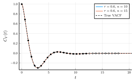
Figure 1: The true VACF and two approximate VACFs for the subdiffusive model. The black points represent the data samples used in the $[0,12]$ grid to approximate the VACF and the white points represent the additional data samples used on the $[0,18]$ grid.

Given the shape of the VACF displayed in Figure 1 we have run our algorithm with data samples for three different grid spacings, i.e., values of $\tau$; for each choice we have compared two grids covering the time interval $[0,12]$ and approximately $[0,18]$, respectively. The corresponding parameter values are

• $\tau=0.4$ with $n=15$ and $n=22$,

• $\tau=0.6$ with $n=10$ and $n=15$,

• $\tau=1.0$ with $n=6$ and $n=9$.

In Figure 1 the target data for $\tau=0.6$ are highlighted (the additional data for the longer time interval are marked in white); besides the exact VACF this figure also shows the corresponding approximations (42) for both associated values of $n$. In this scale the approximations exhibit a perfect fit of the true autocorrelation function. The same is true for all other four aforementioned choices of the two parameters $\tau$ and $n$.

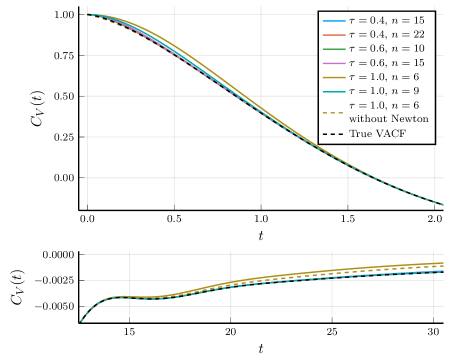
Figure 2: Enlargements of the graph of the subdiffusive VACF and its approximations. The upper panel shows the VACF at short times ($t=0.0$ to $t=2.0$) and the lower panel shows the same VACF at long times ($t=10$ to $t=30$).

A zoom into the approximate VACFs, however, provides some practical guidelines on how to choose $\tau$ and $n$ for a given problem. For example, the reconstructions corresponding to $\tau=1.0$ exhibit a certain misfit near $t=0$ (upper panel in Figure 2), and the one for $\tau=1.0$ and $n=6$ also has difficulties in matching the small wriggle near $t=17$ and the subsequent tail of the true autocorrelation function (bottom panel in Figure 2); all curves that are not visible in these plots lie exactly underneath the true VACF. Such misfits show that the grid spacing $\tau=1.0$ is too large to cope with finer details and the infinite curvature at $t=0$ of the true autocorrelation function.

As a matter of fact, our Prony series approximation for $\tau=1.0$ and $n=6$ fails to correspond to a positive real transfer function and does not lead to a valid Langevin system. For these parameters a modified system (15) with nonzeros in the (1,1)-entry of the system matrix and the top entry of the noise vector can be constructed by dropping constraint (27) (thereby foregoing the Newton iteration), resulting in $\dot{f}(0)=-0.204$. The corresponding approximate VACF is included as dashed line in Figure 2, but is hardly visible in the upper panel, as it is almost enteirely hidden underneath the true VACF; for larger $t$, though, its fit is not much better than the original one according to the lower panel.

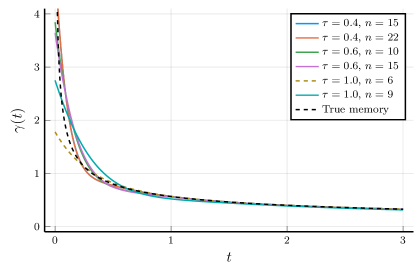
Figure 3: Approximations of the subdiffusive memory kernel.

Figure 3 presents the reconstructed memory kernels (18) for the various combinations of $\tau$ and $n$; again, the dashed line corresponds to the case $\tau=1.0$ and $n=6$ without the constraint (27), where the memory kernel comes with an additional delta distribution at $t=0$. It can be seen that the quality of the approximation increases with reduced grid spacing and with increasing number of grid points.

$\tau$  1.0 1.0 0.6 0.6 0.4 0.4 $n$  6 9 10 15 15 22 $N$  5 8 19 11 10 11

Table 1: Number $N$ of auxiliary variables $Z$ in (15) for different choices of $\tau$ and $n$. The italicized entry $N=5$ in the first column corresponds to the unconstrained VACF approximation.

It is interesting to note that increasing the number of grid points (for the same grid spacing) beyond a certain threshold leads to the occurrence of spurious eigenvalues. As shown in Table 1, when increasing the number of grid points for $\tau=0.6$ from $2n=20$ to $30$, then the size of the Langevin system (15) increases only by two (and not by five, as one would expect). The situation is even more striking for $\tau=0.4$: increasing the number of data points from $2n=30$ to $44$ leads to only one additional auxiliary variable in (15).

3.2 Molecular dynamics data

In earlier work [27] we have employed an MD simulation to generate VACF data of a single colloid in a Lennard-Jones (LJ) fluid. In that work we have developed a new iterative procedure (which we called IMRV method) to determine a memory kernel for a generalized Langevin equation of a coarse-grained model. Here we demonstrate the consistency of the memory kernel (18) corresponding to the extended Langevin model (15) based on our approximation of the same VACF with the results from [27].

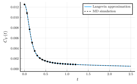
Figure 4: VACF from an MD simulation, with (unnormalized) interpolation, points and the corresponding approximation.

In preliminary experiments we found that in this setup the interpolation grid should extend up to a final time somewhat beyond $t=1$, and therefore we have chosen the parameters $\tau=0.06$ and $n=10$ for this example (see Figure 4). With these parameters we haven’t encountered any spurious eigenvalues nor negative real ones, so the extended system is also of size $10\times 10$ with $N=9$ auxiliary variables.

From Figure 5 it can be seen that the corresponding memory kernel approximation (18) is very similar to the two kernels computed in [27] with the IMRV method and via the (second order) Volterra integral equation scheme suggested in [45].

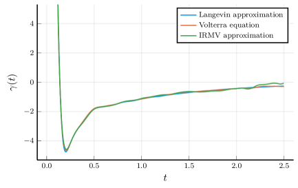
Figure 5: Approximations of the memory kernel for the MD simulation.

3.3 The impact of data noise

To assess how well our method performs with noisy data, we generated three data sets with shorter run times, which results in less smooth VACFs.

The setup of these MD simulations is almost identical to that in the previous section. The system is that of a colloid in a fluid of $N=31627$ LJ particles with size $\sigma$ and mass $m$. We use truncated and shifted LJ potentials with the energy scale $\epsilon$ which are cut off at $r_{\mathrm{c}}=2^{\frac{1}{6}}\sigma$, resulting in purely repulsive WCA interactions. The cubic simulation box has periodic boundary conditions in all three dimensions and a side length $35.76\sigma$. The length, energy, and mass scales in the system are defined by the LJ diameter $\sigma$, energy $\epsilon$, and mass $m$, respectively, which defines the LJ time scale $t_{\mathrm{LJ}}=\sigma\sqrt{m/\epsilon}$. The colloid has a mass of $M=80m$ and is defined as a rigid body with a radius $R=3\sigma$. In these simulations the body of the colloid is constructed so that its surface is more smooth than that of the simulations in [27], resulting in full slip boundary conditions for the LJ fluid. In order to sample at our desired temperature, $\beta=1$, we equilibrate the system with a Langevin thermostat. All simulations are performed using LAMMPS [43].

We have generated three data sets with different levels of noise corresponding to the following production run lengths, where we use a time step of $\Delta t_{\mathrm{MD}}=0.001$:

1. Low noise setting:
   $5$ M steps for the production run;

2. Medium noise setting:
   $1$ M steps for the production run;

3. High noise setting:
   $0.1$ M steps for the production run.

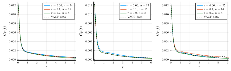
Figure 6: VACF approximations for noisy data sets: (i) left panel, (ii) middle panel, and (iii) right panel.

In Figure 6, it can be seen that the relevant details of the VACF occur in the time interval $[0,3]$, while data noise seems to dominate beyond $t=5$ – in each of the three settings. We therefore found it appropriate to sample interpolation data from about the time interval $[0,3]$, using three different grid spacings:

• $\tau=0.06$ with $n=25$ (50 samples),

• $\tau=0.1$ with $n=15$ (30 samples),

• $\tau=0.2$ with $n=8$ (16 samples).

However, not all transfer functions associated with these data have been positive real; when they weren’t we reduced the dimension $n$ by one, and retried, until being successful eventually.

(i) (ii) (iii) $n$ $N$ $n$ $N$ $n$ $N$ $\tau=0.06$ 24 12 23 12 25 16 $\tau=0.1$ 15 5 15 9 14 7 $\tau=0.2$ 8 3 8 4 8 4

Table 2: Grid parameter $n$ and number $N$ of auxiliary variables $Z$ in (15) for noisy data.

This is documented in Table 2: For example, the entry $n=23$ for the medium noise setting (ii) and grid spacing $\tau=0.06$ bears witness that both for $n=24$ and $n=25$ the corresponding transfer functions failed to be positive real. Overall, out of the $9=3\cdot 3$ cases that we have used data samples for, six have been successful right away, while three of them failed initially, namely setting (i) with $\tau=0.06$, setting (ii) with $\tau=0.06$, and setting (iii) with $\tau=0.1$. It is difficult, though, to deduce a general rule of thumb for when the algorithm is prone to fail. Our experience indicates that the probability increases significantly beyond $n=20$, but the algorithm may break down for $n=25$, and yet be successful for $n=26$.

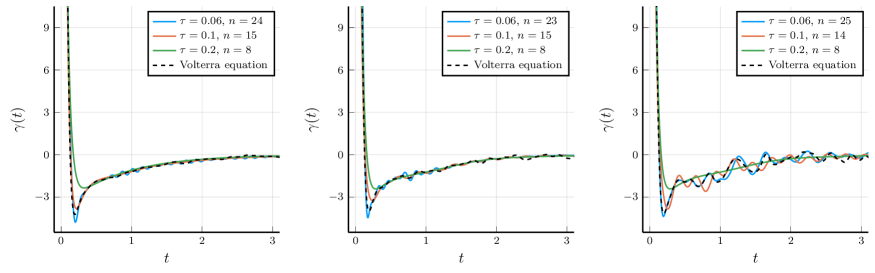
Figure 7: memory approximations for noisy data sets: (i) left panel, (ii) middle panel, and (iii) right panel.

Turning to the VACF plots in Figure 6 it can be seen that in the low and medium noise settings, (i) and (ii), the VACF approximation for the grid spacing $\tau=0.1$ is best, whereas $\tau=0.2$ yields the best result in the high noise setting (iii). The latter is surprisingly smooth in spite of the high amount of noise, and looks very similar to the one from setting (ii). In fact, according to Table 2 both approximations are based on only five ($=N+1$) non-spurious eigenvalues of $A$ and their associated eigenvectors, and those probably carry much the same information in both settings.

Overall we conclude that $\tau=0.06$ is too small for this MD setup: In the high noise setting (iii) the corresponding VACF reconstruction picks up too much noise and is oscillating a lot; in the other two settings the noise doesn’t manifest itself in the reconstruction but in a series of spurious eigenvalues ($N\ll n-1$), the elimination of which causes a certain loss of the interpolation property and restricts the quality of the approximation. This is most striking for the medium noise setting (ii) – which is the example where dimensions $n=25$ and $n=24$ failed.

Concerning the impact of noise on the associated memory terms, Figure 7 reveals that with increasing noise more and stronger oscillations appear in the memory kernels. This effect becomes stronger with decreasing grid width $\tau$, but all Langevin models are more robust in that respect than the Volterra equation method, which we have employed for “calibration”. Taking the kernel calculated with the Volterra method for the small noise setting (i) as “ground truth,” then one can see that the Langevin models for $\tau=0.2$ fail to match the depth of the sharp minimum of the kernel near $t=0.2$, whereas the memory kernels for the other two grids provide a reasonable fit of this particular feature, regardless of the noise magnitude. Apparently, the grid spacing $\tau=0.2$ is too wide for that purpose – although this could not be perceived from the VACF reconstructions. On the other hand, in the high noise setting (iii) the fairly smooth memory for $\tau=0.2$ is the most convincing one. We conclude that for larger amounts of noise it pays off to use a larger grid spacing, and that the quality of the associated memory kernel correlates well with the quality and the smoothness of the VACF approximation.

3.4 Computational efficiency

The accurate determination of an extended Langevin model allows systems to be coarse-grained. However, for such a model to be useful as a coarse-graining tool, it needs to provide a sufficient speedup to simulation runtimes. To evaluate the speedup, we simulate a coarse-grained model of the system discussed in Section 3.3 using the extended Langevin model determined from the method outlined in this paper. We then compare this runtime to that of a fine-grained MD simulation of the same system, using the same time step $\Delta t_{\mathrm{MD}}=0.001$. All simulations are performed in 3-dimensions using LAMMPS [43]. Although the described method is derived in one-dimension, each component of the velocity in our system is uncorrelated. Therefore, we can apply the determined extended Langevin model to each component of the velocity and maintain the system properties. For our coarse-grained simulation, we use an Euler-Maruyama integration scheme.

As expected, simulations using our extended Langevin model were significantly less computationally expensive than the fine-grained MD simulations. The speedup factor per time step was $160$ for an extended Langevin model with $9$ auxiliary variables, and $170$ for a Langevin model with only $5$ variables. Normalizing these numbers by the degree of coarse-graining (i.e., the number of fine-grained particles per coarse-grained particle), these numbers are comparable to those reported by Wang et al. [49], who used their machine learning based auxiliary variable schemes with comparably high number of auxiliary variables to study dilute star polymer solutions. We note that the actual speedup per time unit is even larger due to the fact that the time steps in coarse-grained simulations can be chosen much larger than in microscopic simulations [27, 49].

4 Conclusion

In the present work, we have addressed the problem of mapping GLEs onto equivalent extended Markovian Langevin equations which can be integrated more easily in numerical simulations. We have developed an analytical method to extract the parameters of the extended Markovian system directly from the knowledge of the autocorrelation function of the target quantity, without knowledge of the memory kernel in the GLE. The memory kernel can also be evaluated in retrospect via Eq. (18). Importantly, in contrast to related recent approaches based on auxiliary variables [11, 5, 47, 35, 49], the number of independent degrees of freedom in our extended Markovian system is the same as that in the original GLE. Thus we are not extending the configurational space of the system. Compared to previous methods to derive extended Markovian integrators for GLEs, our method has the advantage that the number of auxiliary variables can be chosen much larger, even beyond twenty in some of our test runs. Therefore, the memory kernel can be represented very accurately. Moreover, as we have shown above, the algorithm can handle input data that suffer from large statistical noise.

We have derived the algorithm using the example of a GLE for Brownian dynamics with memory. In doing so, we have assumed that the derivative of the VACF vanishes at time zero, $\dot{C}_{V}(0)=0$. This is certainly the case if it is derived from an underlying atomistic model with reversible, Hamiltonian dynamics. However, it may not be correct if the underlying fine-grained dynamics already has a dissipative component. From a physical point of view, this would imply that the dynamics of the system is governed by processes on vastly different time scales – intermediate time scales that are captured by the memory kernel, and very short scales that are captured by additional instantaneous friction terms. Our algorithm can be extended to account for such a possibility, as we have demonstrated in Section 3.1.

In the current form, the algorithm can be used to integrate one dimensional GLEs or higher dimensional GLEs, if the memory and stochastic part of the high dimensional GLE can be written as a sum of independent one-dimensional GLEs. This is the case in most current applications of Non-Markovian modelling, e.g., in GLEs based on self-memory only [49] and in Non-Markovian dissipative particle dynamics [33]. In the present form, this method cannot yet be applied to general multidimensional GLEs with pair memory [28]. Extending the algorithm for such cases will be the subject of future work.

Appendix A The Newton scheme

In order to satisfy (27), we consider the (1,1)-entry $A_{1,1}$ of $A$ as a function $\varphi$ of $y_{1}$, choose $y_{1}^{(0)}=y_{1}$ as initial guess, and use the Newton iteration

$$\ y_{1}^{(m+1)}\!=y_{1}^{(m)}-\frac{\varphi(y_{1}^{(m)})}{\varphi^{\prime}(y_{1}^{(m)})}\,,\ \,\nu=0,1,\dots,$$ (53)

until a suitable value $y_{1}^{(m+1)}$ with $\varphi(y_{1}^{(m+1)})\approx 0$ has been found. However, instead of the target function $\varphi(y_{1})=A_{1,1}$, chosen in (27) for the ease of presentation, we (need to) use

$$\ \varphi(y_{1})\,=\,{\rm Re}\,A_{1,1}$$ (54)

in (53). The reason is that negative eigenvalues of $J$ result in a nonzero imaginary part of $A$, and it is only the real part which is relevant for our purpose because of the way we subsequently modify these eigenvalues, see B.

The difficulty in (53) is the evaluation of the derivative $\varphi^{\prime}$ because of the nontrivial recursion that is used to set up the tridiagonal matrix $J$. We resolve this problem in two steps. First, we use algorithmic differentiation [23] to simultaneously determine $J$ and its derivative

$$\ \partial J\,=\,\frac{\rmd J}{\rmd y_{1}}\,\in{\mathord{\mathbb{R}}}^{n\times n}.$$ (55)

Second, we employ the chain rule

$$\ \partial A\,:=\,\frac{\rmd A}{\rmd y_{1}}\,=\,\frac{1}{\tau}\,\frac{\rmd}{\rmd J}\!\log(J)\,\,\partial J$$

and the useful relation

$$\ \log\Bigl{(}\left[\hskip-5.0pt\begin{array}[]{*\c@MaxMatrixCols c}J&\partial J\\ 0&J\end{array}\hskip-5.0pt\right]\Bigr{)}\,=\,\left[\hskip-5.0pt\begin{array}[]{*\c@MaxMatrixCols c}A&\partial A\\ 0&A\phantom{{}^{\prime}}\end{array}\hskip-5.0pt\right],$$ (56)

which follows from [25, p. 58].

This yields the expression

$$\ \varphi^{\prime}(y_{1})\,=\,{\rm Re}\,(e_{1}^{T}\partial A\,e_{1})\,=\,{\rm Re}\,\partial A_{1,1}\,,$$

to be used in (53), see C for further details.

We finally mention that there is no need to determine $y_{1}$ to high accuracy, because (i) the subsequent modifications of $A$, cf. B, will slightly perturb this matrix entry anyway, and (ii) because of the way we (approximately) solve the singular Lur’e equations, cf. C. In our experiments two to seven Newton steps were always sufficient.

Appendix B Spectral modifications of the system matrix

Eliminating spurious exponentials

Given the eigenvector matrix (23) of $A$, we let $z=X^{-1}e_{1}=[z_{1},\dots,z_{n}]^{T}$. Then we readily conclude from (24) the Prony series representation

$$\ f(t)\,=\,e_{1}^{T}Xe^{t\Lambda}X^{-1}e_{1}\,=\,\sum_{j}w_{j}e^{t\lambda_{j}}$$ (57)

of (26) with

$$\ w_{j}=x_{1j}z_{j}\,,$$ (58)

where $x_{1j}$ is the first entry of the $j$th eigenvector $x_{j}$.

Let us now make the assumption that $\lambda_{n}$ is a spurious eigenvalue of $A$ in the closed right-half plane, which we want to eliminate from (57), because it is non-physical and has negligible impact on $f$ for $t\in\triangle$, since $|x_{1n}|$ and $|z_{n}|$ are sufficiently small.

We denote by $\Lambda^{\prime}$ the diagonal matrix with the eigenvalues $\lambda_{1},\dots,\lambda_{n-1}$ of $A$. Then we delete the final column of $X$ and select one out of rows $2$ to $n$, which we also delete from $X$ to obtain an invertible matrix $X^{\prime}\in{\mathord{\mathbb{R}}}^{(n-1)\times(n-1)}$ – in our code we always took the last row. Finally, let $z^{\prime}=[z_{1},\dots,z_{n-1}]^{T}$ and $e_{1}^{\prime}$ denote the first canonical basis vector in ${\mathord{\mathbb{R}}}^{n-1}$. Since $z_{n}$ is assumed to be negligible, it follows that

$$\ X^{\prime}z^{\prime}\,\approx\,e_{1}^{\prime}\,,\quad{\rm i.e.},\quad z^{\prime}\,\approx\,{X^{\prime}}^{-1}e_{1}^{\prime}\,,$$

and hence, for $t\in\triangle$ there holds

$$\ {e_{1}^{\prime}}^{\!T}X^{\prime}e^{t\Lambda^{\prime}}{X^{\prime}}^{-1}e_{1}^{\prime}\,\approx\,{e_{1}^{\prime}}^{\!T}X^{\prime}e^{t\Lambda^{\prime}}z^{\prime}\,=\,\sum_{j=1}^{n-1}w_{j}e^{t\lambda_{j}}$$

by virtue of (58). We therefore achieve our goal by replacing $A$ by

$$\ A^{\prime}\,=\,X^{\prime}\Lambda^{\prime}{X^{\prime}}^{-1}\,.$$ (59)

Treatment of negative eigenvalues of $J$

Recall that we have made the assumption that all eigenvalues of $J$ are different. Let us now assume that the eigenvalue $\mu_{n}$ of $J$ belongs to the interval $(-1,0)$; it comes with a real eigenvector $x_{n}$ and a real weight $w_{n}$ in (57).

In order to replace the corresponding exponential term by the one in (28), we define the diagonal matrix

$$\ \Lambda^{\prime}\,=\,{\left[\hskip-1.29167pt\begin{array}[]{*\c@MaxMatrixCols c}\lambda_{1}&\\[-4.30554pt] &\ddots&\\[-4.30554pt] &&\lambda_{n}\\[-2.15277pt] &&&\lambda_{-n}\end{array}\hskip-1.29167pt\right]}$$

with $\lambda_{\pm n}$ as in (29), and we further let

$$\ X^{\prime}\,=\,\left[\hskip-5.0pt\begin{array}[]{*\c@MaxMatrixCols c}x_{1}&\cdots&x_{n-1}&x_{n}&x_{n}\\ 0&\cdots&0&\rmi&-\rmi\end{array}\hskip-5.0pt\right]$$

and

$$\ z^{\prime}\,=\,\Bigl{[}z_{1}\ \cdots\ z_{n-1}\ \frac{z_{n}}{2}\ \frac{z_{n}}{2}\Bigr{]}^{T}.$$

The matrix $X^{\prime}$ is an invertible $(n+1)\times(n+1)$ matrix, and it satisfies

$$\ X^{\prime}z^{\prime}\,=\,\left[\hskip-5.0pt\begin{array}[]{*\c@MaxMatrixCols c}Xz\\ 0\end{array}\hskip-5.0pt\right]\,=\,\left[\hskip-5.0pt\begin{array}[]{*\c@MaxMatrixCols c}e_{1}\\ 0\end{array}\hskip-5.0pt\right]\,=\,e_{1}^{\prime}\,,$$

where $e_{1}^{\prime}$ is the first canonical basis vector in ${\mathord{\mathbb{R}}}^{n+1}$. It therefore follows that

$$\ {e_{1}^{\prime}}^{\!T}X^{\prime}e^{t\Lambda^{\prime}}{X^{\prime}}^{-1}e_{1}^{\prime}\,=\,{e_{1}^{\prime}}^{\!T}X^{\prime}e^{t\Lambda^{\prime}}z^{\prime}$$

$$\ \,=\,\sum_{j=1}^{n-1}w_{j}e^{t\lambda_{j}}\,+\,\frac{1}{2}\,w_{n}e^{t\lambda_{n}}\,+\,\frac{1}{2}\,w_{n}e^{t\lambda_{-n}}$$

$$\ \,=\,\sum_{j=1}^{n-1}w_{j}e^{t\lambda_{j}}\,+\,w_{n}|\mu_{n}|^{t/\tau}\!\cos(\pi t/\tau)$$

by virtue of (29). Since this is the Prony series we have been looking for, we achieve our goal by replacing $A$ by

$$\ A^{\prime}\,=\,X^{\prime}\Lambda^{\prime}{X^{\prime}}^{-1}\,.$$ (60)

Appendix C Outline of the full algorithm

Algorithm 1  Input: $y_{\nu}=C_{V}(\nu\tau)/C_{V}(0)$, $\nu=0,\ldots,2n-1$

1:call Algorithm 2 to compute the matrix $J$ and its derivative $\partial J$ with respect to $y_{1}$

2:for $i=1,\ldots,i_{\max}$ do

3:    set $\left[\hskip-5.0pt\begin{array}[]{*\c@MaxMatrixCols c}A&\partial A\\ 0&A\end{array}\hskip-5.0pt\right]\leftarrow{\displaystyle\frac{1}{\tau}}\log\left[\hskip-5.0pt\begin{array}[]{*\c@MaxMatrixCols c}J&\partial J\\ 0&J\end{array}\hskip-5.0pt\right]$

4:    set $y_{1}\leftarrow y_{1}-{\rm Re}\,A_{1,1}/{\rm Re}\,\partial A_{1,1}$

5:    call Algorithm 2 to recompute $J$ and $\partial J$ with the new data vector $y$

6:end for

7:if $|A_{1,1}|>\varepsilon$ then

8:    error (Newton’s method did not find a zero of the function $y_{1}\mapsto A_{1,1}$)

9:end if

10:factorize $J=XDX^{-1}$ with a diagonal matrix $D$; $[\mu_{1},\ldots,\mu_{n}]\leftarrow{\rm diag}\,(D)$

11:duplicate eigenvalues $\mu_{j}\in(-1,0)$ and remove eigenvalues $\mu_{j}$ with $|\mu_{j}|\geq 1$;
adjust $X$ and $D$ accordingly (see B)

12:set $\Lambda\leftarrow\frac{1}{\tau}\log(D)$; for duplicated eigenvalues $\mu_{j}\in(-1,0)$ employ formula (29)

13:set $A\leftarrow X\Lambda X^{-1}$

14:set $A_{1,1}=-\delta$ with $\delta>0$ small (e.g., $\delta=10^{-5}$), so that $A=\left[\hskip-5.0pt\begin{array}[]{*\c@MaxMatrixCols c}-\delta&b^{T}\\ -c&A_{0}\end{array}\hskip-5.0pt\right]$

15:solve the Riccati equation (62) for the symmetric and positive semidefinite matrix $\Sigma_{0}$

16:set $\Sigma\leftarrow\left[\hskip-5.0pt\begin{array}[]{*\c@MaxMatrixCols c}1&0\\ 0&\Sigma_{0}\end{array}\hskip-5.0pt\right]$,  $L\leftarrow{\displaystyle\frac{1}{\sqrt{2\delta\beta m}}}\left[\hskip-5.0pt\begin{array}[]{*\c@MaxMatrixCols c}2\delta\\ c-\Sigma_{0}b\end{array}\hskip-5.0pt\right]$

17:if $A\Sigma+\Sigma A^{T}\neq-\beta m\,LL^{T}$ then

18:    error (transfer function is not positive real)

19:end if

20:factorize $A=UTU^{-1}$ (Lanczos algorithm) with

$$\ T=\left[\hskip-5.0pt\begin{array}[]{*\c@MaxMatrixCols c}-\delta&ke_{1}^{T}\\ -ke_{1}&T_{0}^{\prime}\end{array}\hskip-5.0pt\right]\quad\mbox{tridiagonal and}\quad U=\left[\hskip-5.0pt\begin{array}[]{*\c@MaxMatrixCols c}1&0\\ 0&U_{0}\end{array}\hskip-5.0pt\right]$$

21:return $T$ and $G=U^{-1}L$

Algorithm 2  Input: $y_{\nu}$, $\nu=0,\ldots,2n-1$;  $\Phi$ and $\partial\Phi$ are defined in (63) and (64)

1:set $u_{-1}\leftarrow 0$ ,  $\partial u_{-1}\leftarrow 0$

2:set $u_{0}\leftarrow 1/\sqrt{|y_{0}|}$ ,  $\partial u_{0}\leftarrow 0$

3:set $\alpha_{0}\leftarrow y_{1}/y_{0}$ ,  $\partial\alpha_{0}\leftarrow 1/y_{0}$

4:set $\gamma_{0}\leftarrow 0$ ,  $\partial\gamma_{0}\leftarrow 0$

5:set $\sigma_{0}=1$

6:set $J_{1,1}\leftarrow\alpha_{0}$ ,  $\partial J_{1,1}\leftarrow\partial\alpha_{0}$

7:for $i=1,\ldots,n-1$ do

8:    set $\tilde{u}_{i}\leftarrow xu_{i-1}-\alpha_{i-1}u_{i-1}-\sigma_{i-1}\gamma_{i-1}u_{i-2}$

9:    set $\partial\tilde{u}_{i}\leftarrow x\partial u_{i-1}-\bigl{(}\partial\alpha_{i-1}u_{i-1}+\alpha_{i-1}\partial u_{i-1}\bigr{)}-\sigma_{i-1}\bigl{(}\partial\gamma_{i-1}u_{i-2}+\gamma_{i-1}\partial u_{i-2}\bigr{)}$

10:    set $\gamma_{i}\leftarrow\sqrt{|\Phi[\tilde{u}_{i}^{2}]|}$

11:    if $\gamma_{i}=0$ then

12:        error (Lanczos algorithm break down)

13:    end if

14:    set $\partial\gamma_{i}\leftarrow{\displaystyle\frac{{\rm sign}(\Phi[\tilde{u}_{i}^{2}])}{2\gamma_{i}}}\bigl{(}\Phi[2\tilde{u}_{i}\partial\tilde{u}_{i}]+\partial\Phi[\tilde{u}_{i}^{2}]\bigr{)}$

15:    set $u_{i}\leftarrow\tilde{u}_{i}/\gamma_{i}$ ,  $\partial u_{i}\leftarrow{\displaystyle\frac{\partial\tilde{u}_{i}\gamma_{i}-\tilde{u}_{i}\partial\gamma_{i}}{\gamma_{i}^{2}}}$

16:    set $\alpha_{i}\leftarrow\Phi[xu_{i}^{2}]/\Phi[u_{i}^{2}]$

17:    set $\partial\alpha_{i}\leftarrow{\displaystyle\frac{\Phi[u_{i}^{2}]\Phi[2xu_{i}\partial u_{i}]+\Phi[u_{i}^{2}]\partial\Phi[xu_{i}^{2}]-\Phi[xu_{i}^{2}]\Phi[2u_{i}\partial u_{i}]-\Phi[xu_{i}^{2}]\partial\Phi[u_{i}^{2}]}{\Phi[u_{i}^{2}]^{2}}}$

18:    set $\sigma_{i}\leftarrow\Phi[u_{i}^{2}]/\Phi[u_{i-1}^{2}]$

19:    set $J_{i+1,i+1}\leftarrow\alpha_{i}$ ,  $\partial J_{i+1,i+1}\leftarrow\partial\alpha_{i}$

20:    set $J_{i+1,i}\leftarrow\sigma_{i}\gamma_{i}$ ,  $\partial J_{i+1,i}\leftarrow\sigma_{i}\partial\gamma_{i}$

21:    set $J_{i,i+1}\leftarrow\gamma_{i}$ ,  $\partial J_{i,i+1}\leftarrow\partial\gamma_{i}$

22:end for

23:return $J$, $\partial J$

We provide a pseudocode formulation of the overall algorithm in Algorithm 1. For the ease of presentation it comes with a small threshold parameter $\varepsilon$ and a maximum number $i_{\max}$ of iterative steps to control the Newton iteration.

In contrast to our presentation in Section 2.2 we have taken the liberty to introduce in line 14 of Algorithm 1 a negative entry $A_{1,1}=-\delta$ of small absolute value to circumvent the singular Lur’e equations (46); this is a kind of regularization. The associated Lyapunov equation $A\Sigma+\Sigma A^{T}=-\beta m\,LL^{T}$ with $L$ as in line 16 is equivalent to the more amenable (regular) Lur’e equations

$$\eqalign{\ A_{0}\Sigma_{0}+\Sigma_{0}A_{0}^{T}\,=\,-\beta m\,\ell\ell^{T}\,,\cr\ c-\Sigma_{0}b\,=\,\sqrt{2\delta\beta m}\,\ell\,,}$$ (61)

for $\Sigma_{0}$ and $\ell$, cf. [3, 4]. It can be shown that for $\delta\to 0$ the solution of (61) converges to the solution of the corresponding singular Lur’e system (46). Note that when using the second equation in (61) to eliminate $\ell$ from the first one, then this yields the quadratic Riccati equation

$$\ B\Sigma_{0}+\Sigma_{0}B^{T}+\Sigma_{0}bb^{T}\Sigma_{0}+cc^{T}=0\,,\quad B=2\delta A_{0}-cb^{T}\,,$$ (62)

for $\Sigma_{0}$, which is to be solved in line 15. We emphasize that there exists standard software for the solution of this equation, and the same is true for the Lanczos algorithm employed in line 20.

One consequence of introducing the regularization parameter $\delta$ is that the system (15) changes into

$$\ {\rm d}\!\left[\hskip-5.0pt\begin{array}[]{*\c@MaxMatrixCols c}{\tilde{V}}\\ Z\end{array}\hskip-5.0pt\right]\,=\,T\left[\hskip-5.0pt\begin{array}[]{*\c@MaxMatrixCols c}{\tilde{V}}\\ Z\end{array}\hskip-5.0pt\right]{\rm d}t+G\,{\rm d}W\,,$$

where both $T_{1,1}$ and $G_{1}$ are nonzero, but small in absolute value.

Before going on let us define, for polynomials

$$\ p(x)\,=\,\sum_{\nu=0}^{2n-1}a_{\nu}x^{\nu}\,,\quad a_{\nu}\in{\mathord{\mathbb{R}}}\,,$$

of degree $2n-1$, at most, the moment functional

$$\ \Phi[p]\,=\,\sum_{\nu=0}^{2n-1}a_{\nu}y_{\nu}\,,$$ (63)

with $y_{\nu}$ the given data (5). Algorithm 2 determines the corresponding Lanczos polynomials $u_{i}$ of degree $i=0,\dots,n-1$, respectively, given by

$$\ \Phi[u_{i}u_{j}]\,=\,\pm\delta_{ij}\,,\quad i,j=0,\dots,n-1\,,$$

and returns the Jacobi matrix $J$ with the associated recursion coefficients and its derivative $\partial J$ with respect to $y_{1}$. For the computation of this derivative we also introduce the functional $\partial\Phi$ which maps $p$ as above onto

$$\ \partial\Phi[p]\,=\,a_{1}\,.$$ (64)

Note that all variables in Algorithm 2 with a prefix $\partial$ denote the derivative with respect to $y_{1}$ of the same variable without prefix. Further note that $u_{i}$, $\tilde{u}_{i}$, $\partial u_{i}$ and $\partial\tilde{u}_{i}$ are all polynomials of degree $i$ in the real variable $x$, and that, for example, $xu_{i}^{2}$ is short-hand notation for the polynomial $x\mapsto x(u_{i}(x))^{2}$. We finally mention that in line 18 the variable $\sigma_{i}\in\{\pm 1\}$, and hence, its derivative with respect to $y_{1}$ is zero.

References

References

- [1] G Ammar, W Dayawansa, and C Martin, Exponential interpolation: Theory and numerical algorithms, Appl. Math. Comput. 41, pp. 189–232 (1991).
- [2] B D O Anderson, A system theory criterion for positive real matrices, J. SIAM Control 5, pp. 171–182 (1967).
- [3] B D O Anderson, An algebraic solution to the spectral factorization problem, IEEE Trans. Automat. Control 12, pp. 410–414 (1967).
- [4] B D O Anderson and S Vongpanitlerd, Network Analysis and Synthesis: A Modern Systems Theory Approach, Prentice-Hall, Englewood-Cliffs, NJ, 1973.
- [5] A D Baczewski and S D Bond, Numerical integration of the extended variable generalized Langevin equation with a positive Prony representable memory kernel, J. Chem. Phys. 139, 044107 (2013).
- [6] P Benner and M Redmann, Model reduction for stochastic systems, Stoch. PDE: Anal. Comp. 3, pp. 291–338 (2015).
- [7] H Brunner, Volterra Integral Equations: An Introduction to Theory and Applications, Cambridge University Press, Cambridge, 2017.
- [8] A Carof, R Vuilleumier, and B Rotenberg, Two algorithms to compute projected correlation functions in molecular dynamics, J. Chem. Phys. 140, Art.-Nr.124103 (2014).
- [9] M Ceriotti, G Bussi, and M Parrinello, Langevin equation with colored noise for constant-temperature molecular dynamics simulations, Phys. Rev. Lett. 102, Art.-Nr. 020601 (2009).
- [10] M Ceriotti, G Bussi, and M Parrinello, Nuclear quantum effects in solids using a colored-noise thermostat, Phys. Rev. Lett. 103, Art.-Nr. -3-6-3 (2009).
- [11] M Ceriotti, G Bussi, and M Parrinello, Colored-noise thermostats à la carte, J. Chem. Theory Comput. 6, pp. 1170–1180 (2010).
- [12] M Chen, X Li, and C Liu, Computation of the memory functions in the generalized Langevin models for collective dynamcis of macromolecules, J. Chem. Phys. 141, Art.-Nr. 064112 (2014).
- [13] G Ciccotti and J P Ryckaert, Computer simulation of the generalized Brownian motion: I. The scalar case, Mol. Phys. 40, pp. 141–159 (1980).
- [14] D L Ermak and H Buckholz, Numerical integration of the Langevin equation: Monte Carlo simulation, J. Comp. Phys. 35, pp. 169–182 (1980).
- [15] P Feldmann and R W Freund, Efficient linear circuit analysis by Padé approximation via the Lanczos process, IEEE Trans. Comput.-Aided Design Integr. Circuits Syst. 14, pp. 639–649 (1995).
- [16] P Feldmann and R W Freund, Circuit noise evaluation by Padé approximation based model-reduction techniques, in The Best of ICCAD (A Kuehlmann, ed.), Springer, Boston, pp. 451–464 (2003).
- [17] M Ferrario and P Grigolini, A generalization of the Kubo-Freee relaxation theory, Chem. Phys. Lett. 62, pp. 100–106 (1979).
- [18] R W Freund, Model reduction methods based on Krylov subspaces, Acta Numerica 12, pp. 267–319 (2003).
- [19] J Fricks, L Yao, T C Elston, and M G Forest, Time-domain methods for diffusive transport in soft matter, SIAM J. Appl. Math. 69, pp. 1277–1308 (2009).
- [20] W Götze, Complex dynamics of glass-formin liquids – a mode-coupling theory, Oxford University Press, Oxford, 2009.
- [21] I Goychuk, Viscoelastic subdiffusion: Generalized Langevin equation approach, Adv. Chem. Phys. 150, pp. 187–253 (2012).
- [22] H Grabert Projection Operator Techniques in Nonequilibrium Statistical Mechanics, Springer, Berlin, Heidelberg, New Yourk, 1982.
- [23] A Griewank and A Walther, Evaluating Derivatives: Principles and Techniques of Algorithmic Differentiation, 2nd ed., SIAM, Philadelphia, 2008.
- [24] E J Hall, M A Katsoulakis, and L Rey-Bellet, Uncertainty quantification for generalized Langevin dynamics, J. Chem. Phys. 145, 224108 (2016).
- [25] N J Higham, Functions of Matrices: Theory and Computation, SIAM, Philadelphia, 2008.
- [26] F Höfling and T Franosch, Anomalous transport in the crowded world of biological cells, Rep. Progr. Phys. 76, Art.-Nr. 046602 (2013).
- [27] G Jung, M Hanke, and F Schmid, Iterative reconstruction of memory kernels, J. Chem. Theory Comput. 13, pp. 2481–2488 (2017).
- [28] G Jung, M Hanke, and F Schmid, Generalized Langevin dynamcis: Construction and numerical integration of Non-Markovian particle-based models, Soft Matter 14, pp. 9368–9382 (2019).
- [29] T Kinjo and S Hyodo, Equation of motion for coarse-grained simulation based on microscopic description, Phys. Rev. E 75, 051109 (2007).
- [30] L Komzsik, The Lanczos Method: Evolution and Application, SIAM, Philadelphia, 2003.
- [31] B Kowalik, J O Daldrop, J Kappler, J C F Schulz, A Schlaich, and R R Netz, Memory-kernel extraction for different molecular solutes in solvents of varying viscosity in confinement, Phys. Rev. E 100, 012126 (2019).
- [32] H Lei, N A Baker, and X Li, Data-driven parameterization of the generalized Langevin equation, Proc. Natl. Acad. Sci. USA 113, pp. 14183–14188 (2016).
- [33] Z Li, H S Lee, E Darve, and G E Karniadakis, Computing the non-Markovian coarse-grained interactions derived from the Mori-Zwanzig formalism in molecular systems: Application to polymer melts, J. Chem. Phys. 146, 014104 (2017).
- [34] E Lutz, Fractional Langevin equation, Phys. Rev. E 64, 051106 (2001).
- [35] L Ma, X Li, and C Liu, From generalized Langevin equations to Brownian dynamics and embedded Brownian dynamics, J. Chem. Phys. 145, Art.-Nr. 114102 (2016).
- [36] L Ma, X Li and C Liu, The derivation and approximation of coarse-grained dynamics from Langevin dynamics, J. Chem. Phys. 145, 204117 (2016).
- [37] F Marchesoni and P Grigolini, On the extension of the Kramers theory of chemical relaxation to the case of nonwhite noise, J. Chem. Phys. 78, pp. 6287–6298 (1983).
- [38] R Metzler and J Klafter, The random walk’s guide to anomalous dynamics: a fractional dynamics approach, Phys. Rep. 339, pp. 1–77 (2000).
- [39] H Meyer, T Voigtmann, and T Schilling, On the non-stationary generalized Langevin equation, J. Chem. Phys. 147, Art.-Nr. 214110 (2017).
- [40] H Mori, Transport, collective motion, and Brownian motion, Progr. Theor. Phys. 33, pp. 423–455 (1965).
- [41] H Mori A continued-fraction representation of the time-correlation functions, Progr. Theor. Phys. 34, pp. 399-416 (1965).
- [42] G A Pavliotis, Stochastic Processes and Applications. Diffusion Processes, the Fokker-Planck and Langevin Equations, Springer, New York, 2014.
- [43] S Plimpton, Fast parallel algorithms for short-range molecular dynamics, J. Comp. Phys. 117, pp. 1–19 (1995).
- [44] N Pottier, Nonequilibrium Statistical Physics: Linear Irreversible Processes, Oxford University Press, Oxford, 2010.
- [45] H K Shin, C Kim, P Talkner, and E K Lee, Brownian motion from molecular dynamics, Chem. Phys. 375, 316–326 (2010).
- [46] D H Smith and C B Harris, Generalized Brownian dynamcis. I. Numerical integration of the generalized Langevin equation through autoregressive modeling of the memory function, J. Chem. Phys. 92, pp. 1304–1311 (1990).
- [47] L Stella, C D Lorenz, and L Kantorovich, Generalized Langevin equation: An efficient approach to nonequilibrium molecular dynamics of open systems, Phys. Rev. B 89, Art.-Nr. 134303 (2014).
- [48] J M Varah, On fitting exponentials by nonlinear least squares, SIAM J. Sci. Stat. Comput. 6, pp. 30–44 (1985).
- [49] S Wang, Z Ma, and W Pan, Data-driven coarse-grained modeling of polymers in solution with structural and dynamic properties conserved, Soft Matter 16, 8330 (2020).
- [50] A D Viñales and M A Despósito, Anomalous diffusion: Exact solution of the generalized Langevin equation for harmonically bounded particle, Phys. Rev. E 73, 016111 (2006).
- [51] Y Yoshimoto, Z Li, I Kinefuchi, and G E Karniadakis, Construction of non-Markovian coarse-grained models employing the Mori-Zwanzig formalism and iterative Boltzmann inversion, J. Chem. Phys. 147, 244110 (2017).
- [52] R Zwanzig Memory effects in irreversible thermodynamics Physical Review 124, pp. 983–992 (1961).
- [53] R Zwanzig Nonequilibrium statistical mechanics, Oxford University press, New York, 2001.