Universality in Phyllotaxis: a Mechanical Theory

Abstract: One of humanity’s earliest mathematical inquiries might have involved the geometric patterns in plants. The arrangement of leaves on a branch, seeds in a sunflower, and spines on a cactus exhibit repeated spirals, which appear with an intriguing regularity providing a simple demonstration of mathematically complex patterns. Surprisingly, the numbers of these spirals are pairs of Fibonacci numbers consecutive in the series 1, 2, 3, 5, 8, 13, 21, 34, 55… obeying a simple rule 1+2=3, 2+3=5, 5+8=13 and so on. This article describes how physics helps to clarify the origin of this fascinating behavior by linking it to the properties of deformable lattices growing and undergoing structural rearrangements under stress.

published in: Symmetry in Plants, Series in Mathematical Biology and Medicine, eds. R. V. Jean, D. Barabé, (World Scientific Pub Co Inc, 1998)

I Introduction

I.1 The patterns of repetitions in plants

The visual beauty of plants comes, in part, due to the highly regular and well organized patterns of leaves, florets, seeds, scales and other structural units. Widely admired, the regular patterns in plants are not merely aesthetically pleasing, they often have unexpected relation with mathematics. Here we will be concerned with one particular kind of such patterns — the spirally, or helical, arrangements. Spirally patterns occurring in plants have long been known to have a surprising connection with number theory. The area of botany that studies such patterns is called phyllotaxis (the word can be translated as “leaf arrangement”). It has been recognized long ago that the so-called Fibonacci sequence: 1, 2, 3, 5, 8, 13, 21, 34, 55, 89 …, where every number in the sequence appears as a sum of two preceding numbers, is of great importance in phyllotaxis. The prominence of Fibonacci numbers in phyllotaxis is well accounted for in both specialized and popular literature, which includes the gems such as “On Growth and Form” by D’Arcy Thompson D'ArcyThompson and “Symmetry” by H. Weyl Weyl .

The connection between Fibonacci numbers and helical packings of units in plants, which is at the heart of the subject of phyllotaxis, appear to be quite general, although the details depend somewhat on the plant geometry. In cylinder-shaped objects, such as fir-tree cones or pineapples, the scales have a regular arrangement in which two families of helices can be identified, having the right and left helicity. These are known in the literature as parastichy helices wiki_parastichy (see Fig. 1a). The numbers of helices in each family are invariably found to be the Fibonacci numbers. Moreover, the numbers of the right and left helices are non-equal and are given by the pairs of Fibonacci numbers consecutive in the sequence, such as (2,3), (3,5), (5,8), (8,13) and so on. Geometrically, such structures can be described as lattices on the surface of a cylinder. The appearance of Fibonacci numbers in a cylindrical structure is called cylindrical phyllotaxis.

Another type of phyllotactic patterns occurs when units of a plant are packed on a disk. For example, in a sunflower or a daisy, the lines connecting neighboring florets define two families of parastichy spirals wiki_parastichy . Again, in each family the number of spirals is Fibonacci, and in the two families the numbers are consecutive in the sequence (Fig. 1(b)). For such structures, it is common to use the name spiral phyllotaxis. A detailed discussion of the two geometric models of phyllotaxis, cylindrical and spiral, can be found in the article by Rothen and Koch RothenKoch .

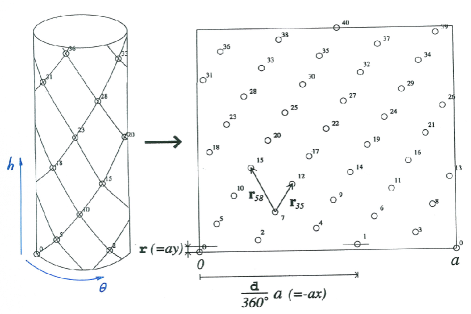
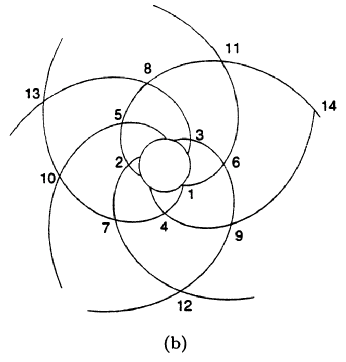
Figure 1: (a) Geometric model of a cylindrical plant, such as a pineapple or a pine cone. The lines connecting neighboring scales form two families of parastichy helices with the right and left helicity. Each family contains a Fibonacci number of helices. The figure illustrates a model of such a structure by a lattice on a cylinder of circumference $a$, and its mapping onto a periodic lattice in the plane. The two lattice vectors are shown that connect the nearest and next-nearest neighbors, and define parastichy helices, The divergence angle ${\sf d}$ and the helix rise ${\sf r}$ are defined in Eq.(1); the parameters $x=-{\sf d}/2\pi$ and $y={\sf r}/a$ are defined in Eq.(4). (b) Geometric model of a plant with a disk geometry, such as a sunflower. The lines connecting neighboring florets generate two families of parastichy spirals of the right and left helicity. The figure illustrates a model of the floret arrangement by a spiral lattice. The points on the spirals are numbered according to the distance from disk center.

The first studies of phyllotaxis probably go back to the observation made by Leonardo da Vinci (notebook, 1503) who noted that

Nature has arranged the leaves of the latest branches of many plants so that the sixth is always above the first, …

(Here $6-1=5$, a Fibonacci number.) Since then, phyllotaxis has had a long and interesting history, excellent reviews of which are given, e.g., by Adler AdlerI , Jean JeanReview , and Lyndon Lyndon . The regularity of the arrangement of leaves and other similar structures fascinated many biologists, mathematicians, crystallographers, and physicists, who were interested in this phenomenon and contributed to the development of the subject. Many renowned scientists contributed to our understanding of phyllotaxis, including Kepler, Linnaeus, Bonnet, Bravais, Airy, among others. Here, instead of reviewing the historical development of the subject, we simply summarize, in a roughly chronological order, the main logical steps of five hunder years of the research in phyllotaxis:
(a) discovering phyllotactic patterns (XV-XVI century);
(b) observing and characterizing (XVI-XVIII century);
(c) geometric modeling (since XVIII century);
(d) experimental studies (since XIX century);
(e) interpreting, explaining (since the late XIX century).

Remarkably, after five centuries of inquiry phyllotaxis continues to be an active research area. The reason for that can be seen in its multidisciplinary character. It is a problem that does not belong entirely to any particular branch of science, but has roots in the subjects as diverse as biology, mathematics, and physics. The timeline above makes it evident how these disciplines, as they progressed, have found application in phyllotaxis by prompting new questions motivated by their own logic and providing new valuable perspective on an old problem.

I.2 Why Fibonacci numbers?

In the XX century the trends and interests in this field focused on the question of the origin of phyllotaxis. Here is how the challenge was stated by a mathematical biologist:

The fascinating question: “Why does the Fibonacci sequence arise in the secondary right or left spirals seen on plants?” seems to be at the heart of problems of plant morphology. In atomic physics, Balmer’s series has opened the way to Bohr’s theory of the atom and then to quantum mechanics and to quantum electrodynamics. The great hope of bio-mathematicians is that some day they may be able to do for biology what has been done by mathematical physicists in physics. (R. V. Jean, Ref. JeanJTB , p. 641)

Indeed, despite the long history, no general agreement was reached with regard to the origin of phyllotaxis. Many explanations proposed in the past simply state that the Fibonacci packings are optimal in some sense. Already Leonardo, after noticing the regularity in the numbers of leaves, remarks that the reason they are arranged in such a way probably has something to do with a better exposure to the sun light through minimizing mutual shadowing. Later, the logic of the discussion of the origin of phyllotaxis basically followed that of Leonardo’s, by adding more optimization factors, such as air circulation in between the leaves, or the density of packing of the seeds or florets. The review of such theories can be found, for example, in the D’Arcy Thompson’s book D'ArcyThompson . The Darwinian evolutionary theory, by asserting that natural selection gives rise to the optimal structures that are better designed for a local environment, apparently endows such theories with an air of confidence.

However, such views are known to be at odds with certain experimental observations. Indeed, as emphasized in the evolutionary theory, the evolutionary pressure arises from variability within the species. Namely, if the species are optimized with respect to a certain factor by evolutionary pressure, there must also occur, however rarely, the species that are not optimal but near-optimal. If this was the case in the phyllotactic growth, a sunflower that normally exhibits 55 spirals could sometimes have 54 or 56 spirals. In other words, the most frequent kind of an exception from the Fibonacci rule would be associated with the numbers that are close but not equal to the Fibonacci numbers. And yet such numbers never occur; instead a very different kind of non-Fibonacci patterns is observed. The most common exception known to occur is described by the numbers from the so-called Lucas sequence Weyl : 1, 3, 4, 7, 11, 18, 29 … . The sequence is constructed according to the Fibonacci addition rule, however it starts with a different pair of numbers. Another aspect of phyllotaxis that seems to be hard to reconcile with the evolutionary optimization theories, is that the non-Fibonacci numbers patterns, even those of the most common Lucas type, occur extremely rarely, with the probability of few percent or lower.

The high stability of Fibonacci numbers could make one suspect that perhaps they are in some way “programmed.” However, the conjecture that these numbers are merely encoded genetically seems improbable, because individuals within the same species often exhibit different Fibonacci numbers, but hardly ever the non-Fibonacci (Lucas) numbers. Moreover, as in the case of spiral phyllotaxis, different Fibonacci numbers can occur within one plant. In addition, by simply making reference to genes one does not come closer to the understanding exactly what is special about these numbers. Thus one is led to seek an explanation elsewhere.

In this article we review a mechanical theory Levitov1 ; Levitov2 that establishes a general physical mechanism of phyllotactic growth. Namely, we consider the role of mechanical stresses in a densely packed arrangement of units in a growing plant. The stresses, which build up due to the growth anisotropy, lead to a shear strain in the structure increasing gradually and then relaxing by a sequence of abrupt structural rearrangements. As demonstrated below, this simple mechanical process gives rise, exclusively and deterministically, to Fibonacci structures.

The mechanical explanation of phyllotaxis, which links Fibonacci numbers to transitions in the system upon stress build-up in the process of growth, is completely general and robust. In particular, these transitions are insensitive to the specific form of interactions and, occurring one after another, generate the entire sequence of Fibonacci structures. Further, besides establishing the prevalent character of Fibonacci numbers in phyllotactic patterns the mechanical theory explains why the exceptions are predominantly of a Lucas type. This is achieved by allowing irregularities (e.g. due to fluctuations or noise) to trigger a single mistake at an early growth stage. All predictions of the mechanical theory are therefore in agreement with the observations.

Besides the mechanical scenario of phyllotaxis reviewed in this article, several other approaches focused on various physical growth-related effects that may lead to phyllotaxis. Those include theories of growth mediated by a diffusion of inhibitor (Mitchison Mitchison ), by a reaction-diffusion process (Meinhardt Meinhardt ), and by mechanical interactions that control the largest available space (Couder and Douady CouderDouady ). Some of these theories are discussed in other chapters of this volume.

Are the mechanisms emphasizing different physical processes mutually exclusive or complementary to one another? On a first thought it may appear that, given the clear differences between these approaches, identifying the right mechanism will invalidate other explanations. Yet, below we argue that the situation is considerably more interesting. Our analysis of mechanical stresses and their impact on growth establishes the property of robustness. The robustness basically means a wide stability of phyllotactic patterns with respect to parameter variation in the model. The stability property, by an extension, suggests that there is a degree of truth in all theories which invoke some form of repulsion/stress during growth — mechanical, chemical, or else. In other words, all theories of phyllotaxis which use lattices of objects with some kind of repulsive interactions, no matter the origin and specific geometry (e.g. cylinder, disk, or cone), are equivalent in a “coarse-grained” sense. The situation here is similar to that in the theory of pattern formation, where many different microscopic models are known to lead to identical types of patterns on a larger scale. In physicist’s language, such models, while different in details, belong to the same universality class.

At the same time, there is an open question of comparing the proposed scenarios with the underlying physiological processes in biological systems. This is a fascinating experimental problem that will have to be addressed by future work. However, whatever the outcome of these studies might be, it is worth noting that phyllotactic growth occurs in a large variety of biological systems. It is therefore possible that no unique physiological process applicable to all systems will emerge, and instead several different microscopic scenarios must be considered. At the same time, the robustness of phyllotactic growth, as established in the mechanical theory, will ensure that the resulting patterns are insensitive to the microscopic details of the growth.

This article is organized as follows. In Sec. II we summarize the mechanical theory of phyllotaxis and provide a brief review of its history. In Sec. III we introduce a geometric model that involves cylindrical lattices and families of parastichy helices, defined in terms of the shortest lattice vectors. In this section the notion of a phase space of all cylindrical lattices is defined, which will be central in our subsequent discussion. Next, in Sec. IV we introduce the energy model, and consider its symmetries. These symmetries are found to form a large family, described as an infinite group of modular transformations. Then, in Sec. V the main result of this article is derived. We use the modular symmetries to relate different growth stages and thereby show that Fibonacci numbers are universal in phyllotaxis. This result, established within the energy model, is cast in a rigorous form of a theorem. From the discussion in Sec. V the robustness property of phyllotactic growth becomes evident. In Sec. VI we discuss possible modifications of the model which can bring it closer to other growth geometries, such as those of spiral phyllotaxis, and argue that the stability of Fibonacci patterns and their universality remain unaffected.

II Mechanical theory

II.1 Growth under stress

The mechanical model discussed here involves, in its simplest form, a regular cylindrical lattice of repulsively interacting objects (see Fig. 1a). Cylindrical lattices provide a convenient representation for a wide variety of phyllotactic patterns. Crucially, in this model the lattices are taken to be deformable, with the lattice geometry not fixed rigidly but instead controlled by the balance between external forces and repulsive interactions between different lattice points. The repulsion can be chosen so that it mimics the contact rigidity of the structural units of a plant. However, rather than restricting the repulsive interaction to be a short-range type, it is beneficial to consider a generic repulsive interaction which includes both the short-range and the long-range parts.

Further, the effects of growth can be naturally incorporated in the cylindrical lattice model through an external force applied along the cylinder axis, which gradually increases as the growth progresses. The uniaxial stress due to such a force mimics the stresses arising in the growth of an elongated object in the presence of the closed-volume or confinement constraints. As we will see, under the uniaxial stress the system deforms in such a way that, starting from a simplest quasi-one-dimensional chain-like structure, it goes through the sequence of Fibonacci phyllotactic patterns in a completely deterministic way.

In the mechanical model of phyllotaxis a cylindrical lattice deforms upon a gradual increase in stress; this deformation is described in terms of a gradually developing shear that tends to minimize the total repulsion energy at each given stress value. It is crucial, however, that in such a process the structure does not track the global energy minimum. The reason is that in optimizing its energy the system can explore only the nearby states by developing small deformations in the lattice. Therefore, the Fibonacci structures, appearing upon a gradual increase of the stress, characterize the progression, or time sequence, of deformation, rather than the result of global energy minimization. The Fibonacci structures emerge in this framework as the stages of rearrangement in a deformable system, starting from a certain simple structure and appearing one by one upon an increase in the stress during the growth.

In treating the problem quantitatively, the first step is to define the mechanical energy of a lattice using a model interaction between lattice points, and use this interaction to study the system evolution under stress (see Secs. III,IV). This analysis, which is straightforward to carry out numerically Levitov1 , reveals a very robust behavior: for a variety of repulsive interactions, increasing the stress drives the system through all Fibonacci structures, exclusively and without exceptions. Further, the model has a distinct advantage in that it can be treated analytically for a large family of interactions (see Sec. V). In this case the robustness and universality of Fibonacci structures can be established rigorously Levitov2 . We subsequently argue (Sec. VI), using the robustness property, that the results obtained for cylindrical geometry can be generalized to the disk geometry.

Anisotropic mechanical stress accompanying the growth is a key ingredient of the theory of phyllotaxis advocated in this article. What can be the origin of such a stress? In that regard we note that, while the required stress cannot originate from isotropic hydrostatic pressure, any growth anisotropy can in general lead to anisotropic stresses of the form that generate phyllotaxis. The details of the relationship between the growth anisotropy and stress depend on the specifics of the system at hand and, in particular, the system geometry. However, as argued below, these details are inessential for understanding the general relation between the stress buildup during growth and the formation of phyllotactic patterns.

The relation between anisotropic growth and mechanical stresses is most clear for the growth of a cylindrical structure. Consider a cylindrical lattice, such as that pictured in Fig. 1a, which is growing while being encapsulated in a fixed volume. Such growth can describe, for instance, the early developmental stages of objects like pine tree cones, which have a growth center at the apex. At the growth center, new structural units of the would-be cone are produced at a constant rate, and as a result the cone extends forward. In free space, such a growth would yield one-dimensional chain-like structures. However, if the growth is taking place within a closed volume, the growing cone, or a similar cylindrical object, soon meets a constraint (namely, a boundary) which does not allow it to freely extend forward. As a result, as more and more units are generated at the growth center, the cone will deform in order to fit inside the enclosure. It is instructive to characterize the result of such deformation by rescaling to fixed density on the cylindrical surface (see Fig. 1a). Upon such rescaling, the growth can be described as a gradual expansion in the direction transverse to the cylinder axis accompanied by compression along the axis, such that the two-dimensional areal density remains fixed. As the our analysis below predicts, such a process leads to, exclusively, the Fibonacci structures. The actual numbers achieved will depend on the growth duration: the longer the growth continues, the higher are the Fibonacci numbers that can be accessed.

What are the implications of the behavior found in cylindrical lattices for other geometries of interest? A useful example that helps to answer this question is the growth of a circular object in a disk geometry, as illustrated in Fig. 1b. Such a growth, e.g. describing the development of a sunflower or a daisy, has its center at the center of the disk. During the growth, as more units (e.g. florets) are added at the center, they push the previously added units, forcing them to move outwards along the disk radius. One can argue that this process leads to transformations of the structure equivalent to those of a deformable cylindrical lattice.

This can be done, e.g., by focusing on the evolution of a small rectangular patch of the structure, a distance $r$ away from the center. Namely, one can choose the rectangle sides to be aligned with the cylindrical coordinates, radial and azimuthal, equal to $\delta r$ and $r\delta\theta$, respectively, and consider how they change upon growth. As the growth progresses, this patch moves radially to a new location $r^{\prime}>r$, where the new sides of the rectangle become $(r/r^{\prime})\delta r$ and $r^{\prime}\delta\theta$, since the rectangle angular dimension $\delta\theta$ and its area $r\delta r\delta\theta$ remain constant. The rectangle aspect ratio $r\delta\theta/\delta r$ increases thereupon by a factor $(r^{\prime}/r)^{2}$. As a result, the part of the lattice within the rectangle, after moving from $r$ to $r^{\prime}\gg r$, is strongly deformed. The deformation degree $(r^{\prime}/r)^{2}$ gradually increases along the radius, whereas the areal density of the florets remains roughly constant. Which implies that, since the main forces in the system are due to nearest neighbors exerting pressure on each other, locally the mechanics of the deformed spiral lattice is similar to that of a cylindrical lattice. To map one problem to the other, we can simply replace the spirals of the disk by the helices of the cylinder, which gives a one-to-one relation between the parastichy lines connecting the adjacent lattice points. One unique aspect of the disk growth geometry that distinguishes it from cylindrical geometry is that the deformation varying as a function of radius, as discussed above, gives rise to structural transitions and different phyllotactic domains occurring within the same disk (see discussion in Sec. VI). The concentric annulus-shaped phyllotactic domains have the numbers of spirals (parasticies) which are smaller for the inner domains and greater for the outer domains, increasing with radius (see Sec. VI.2). The numbers of spirals, which are Fibonacci numbers, are therefore largest near the disk edge.

Another geometry of interest corresponds to the growth of a plant at an apex of its shoot. In this case, the growth center where new units of a plant (e.g. leaves, scales, or spines) are generated is located at the center of the rounded top part of a shoot. The geometry of a curved cone describing such a growth can be viewed as intermediate between the disk and cylinder geometries discussed above. Near the growth center, the growth process can be described by the disk geometry, whereas some distance away from it, as the shape of the shoot is curved towards a cylinder, it resembles the cylindrical growth. As in the disk growth case, a thicker shoot gives rise to bigger Fibonacci numbers.

These three basic growth geometries represent different varieties of the general problem of a deformable lattice growing under stress. All three exhibit a very similar behavior. While in each case there are specifics that lead to some modifications in the description of the growth, they do not affect the stability of Fibonacci numbers. The developmental stability follows from the robustness of the sequence of structural changes induced as the mechanical deformation increases under stress (see Sec. VI). This property is central to understanding the universality of Fibonacci patterns.

II.2 Early mechanical scenarios

The first suggestion that mechanical forces play a key role in phyllotaxis seems to have been made by Hubert Airy. In his work “On Leaf-arrangements” (Ref. Airy , p.177) he wrote:

Take a number of spheres (say oak-galls) to represent leaves, and attach them in two rows in alternate order (1/2) along opposite sides of a stretched india-rubber band. Give the band a slight twist to determine the direction of the twist in the subsequent contraction, and then relax the tension. The two rows of spheres will roll up with a strong twist into a tight complex order, which, if the spheres are attached in a close contact with the axis, the order becomes condensed into (nearly) 2/5, with great precision and stability. And it appears that further contraction, with increased distance of the spheres from the axis, will necessarily produce the order (nearly) 3/8, 5/13, 8/21, etc. in succession, and that these successive orders represent successive maxima of stability in the process of change from the simple to the complex.”

This description contains the key element of the mechanical theory: a spiral structure of rigid objects that deforms under a stress. However, the way it is described does not make it clear why such a process leads exclusively to Fibonacci numbers. Moreover, Airy’s statement seems to be more of a conjecture rather than a conclusion, since the analysis verifying this suggestion has not been done at the time. To put these ideas on a firm ground a theory of the development of a spiral structure under mechanical stress is needed.

An important step in this direction was made by van Iterson Iterson . As a starting point, he considered cylindrical lattices, a geometric model that has been used to describe phyllotactic patterns since the work of Bravais Bravais , to which van Iterson added a new ingredient. As in the earlier work, a plant is represented as a cylinder with a spiral arrangement of lattice points on the surface of a cylinder. In that, the lattice points represent individual units of a plant such as leaves, scales, or spines (see Fig. 1). etc. The lattice points, if ordered according to their relative heights along the cylinder axis, $h_{m}$, $m=0,\pm 1,\pm 2...$, can be described geometrically as a set of points on a single generating helix:

$$h_{m}={\sf r}\,m,\quad\theta_{m}=\,{\sf d}\,m,$$ (1)

where ${\sf r}$ is the rise of the helix, and ${\sf d}$ is the angular step known as the divergence angle in the literature. The quantities $h$ and $\theta$, and the lattice points labeled by $m$, are illustrated in Fig. 1a; here all lattice points are assumed to have different height values $h_{m}$. The new ingredient of van Iterson’s model is identical disks centered at the lattice points, with the arrangement of the disks constrained by the dense packing requirement. Namely, the disks are packed in a lattice such that each disk is in a direct contact with at least four nearest-neighbor disks which touch but do not overlap.

The densely packed disks resemble the densely packed structural units of a plant, defining the families of right and left parastichy helices which connect the nearest-neighbor lattice points as illustrated in Fig. 1a. The numbers of the helices in the two families define the cylindrical lattice “parastichy type”. (This model, and in particular the relation of the pairs $({\sf r},{\sf d})$ to the hyperbolic plane, will be discussed in greater detail in Sec. III.) Van Iterson noticed that the dense packing requirement constrains the disk arrangements in a very special way. He demonstrated that the lattices of densely packed disks, when described in terms of the generating helix, Eq.(1), define possible pairs $({\sf r},{\sf d})$ that form a branching structure known as the Cayley tree (see Fig. 2). The Cayley tree consists of the arcs of circles in the $({\sf r},{\sf d})$ plane connected with each other at the triple branching points occurring at the ends of the arcs. The triple branching points correspond to the maximum-density disk packing — the symmetric triangular lattices in which each disk makes contact with exactly six neighbors. Further, the Cayley tree helps to understand the properties of the densely packed disk lattices encoded in their parastichy types — the numbers of the right and left helices which are uniquely determined by the values of ${\sf r}$ and ${\sf d}$.

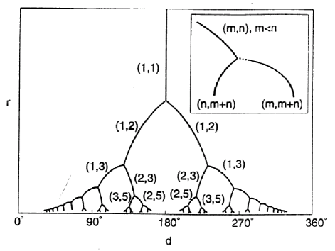
Figure 2: Van Iterson diagram of pairs $({\sf r},{\sf d})$ corresponding to dense packing of disks Iterson . The diagram has a structure of a Cayley tree with the branching number $z=3$. Parastichy pairs (the numbers of the right and left helices) are shown next to each arc.   Inset: The contact pressure theory by Adler AdlerII predicts lifting of the 3-fold symmetry at the branching points by opening gaps in some of the arcs. The dotted line represents unstable disk packings with negative contact pressure.

These numbers show an interesting behavior when placed on the corresponding branches of the Cayley tree. First, the numbers do not change within one branch. Each branch can therefore be labeled by a single pair of integers $(n_{1},n_{2})$. This is illustrated in Fig. 2 where these numbers are shown next to the corresponding Cayley tree branches. Second, as noted above, the triple branching points correspond to perfect triangular lattices of maximum density. Since in a perfect triangular lattice there are three shortest lattice vectors of equal length, and thus three distinct families of helices associated with these vectors, each branching point of the Cayley tree is naturally labeled by three integers $(n_{1},n_{2},n_{3})$. As discussed below, these integers obey the identities $n_{1}+n_{2}=n_{3}$, up to a permutation, which might suggests a link to the Fibonacci series.

Is there a relation between this construction and Fibonacci numbers? A quick inspection of Fig. 2 indicates that the numbers labeling the arcs are in general non-Fibonacci, with the Fibonacci numbers found only in a small subset of the tree. At the same time, the arcs that are labeled by the pairs of Fibonacci numbers form two continuous paths going from the Cayley tree top all the way down to the bottom. Along these paths the pairs of consecutive Fibonacci numbers are found $(1,2)$, $(2,3)$, $(3,5)...$, and $(2,1)$, $(3,2)$, $(5,3)...$; the numbers grow as the rise parameter ${\sf r}$ of the generating helix decreases. Taking the decrease in ${\sf r}$ to be associated with the plant growth (e.g., see Ref. Meicenheimer ), it is tempting to conjecture that the arcs of the Fibonacci paths are somehow linked to different stages of the growth.

These observations were first connected to the effects of mechanical stress by Adler AdlerII . He considered a force that is being applied to a cylindrical lattice along the cylinder axis and increases gradually. Under growing stress the lattice deforms so that the rise of the helix ${\sf r}$ gradually diminishes. In the disk model the effect of growing stress is accounted for by a gradual downward movement along the Cayley tree of the point $({\sf r},{\sf d})$ that represents the lattice. As ${\sf r}$ decreases, the evolution of the point $({\sf r},{\sf d})$ tracks one of the tree branches until a branching point is reached. At which point the system must choose between the two arcs going further down. If we assume that the system, represented by the point $({\sf r},{\sf d})$, would always choose, by some mechanism, to evolve from the branching point along the arc marked by a pair of Fibonacci numbers, the model would predict phyllotactic growth. However, in the original formulation of the disk model it was unclear what mechanism could guide the growth in the right direction at the branching points.

Adler proposed to replace the purely geometric condition of a dense packing of the disks by a more physical notion of an external pressure which is applied to the system of rigid disks and is balanced by the contact pressure between the disks (see also  Schwendener ). The contact pressure theory “resolves” the triple points on the Cayley tree diagram; this happens because the condition for mechanical equilibrium predicts that one of the arcs that meet at each branching point represents a system with negative contact pressure. The negative pressure regions correspond to unstable structures and must be eliminated from the diagram. This leads to gaps opening in the arcs which divide the tree into separate paths of arcs that run downward (see inset of Fig. 2). The evolution along each of these paths, owing to the absence of branching, is deterministic. Further, the two Fibonacci paths discussed above remain unaffected by the negative pressure gaps. Now, as ${\sf r}$ diminishes, the system can evolve through the sequence of Fibonacci states in a perfectly deterministic fashion. (Further details of this construction are discussed in the chapter by Adler in this volume.)

To summarize this discussion, by introducing contact pressure between the disks Adler completed and solved van Iterson’s disk model. His solution provided a proof of phyllotaxis for the contact-pressure interaction. While realistic, this interaction is not found in any biological system. Moreover, since the phenomenon of phyllotaxis is so widespread, and the form of interaction presumably varies strongly among different species, a solution for a particular interaction only partially addresses the problem, leaving the question of robustness unanswered. Proving the universality of phyllotaxis requires establishing the stability of Fibonacci growth in a sufficiently generic class of models.

This is precisely what is accomplished by the energy model Levitov1 ; Levitov2 . The energy model is essentially a generalized contact pressure model, with the contact interactions between disks replaced by a generic repulsive interaction between points of a cylindrical lattice. A big advantage of the energy model is that it cleanly delineates the physics ingredients (interactions) from the geometry ingredients (cylindrical lattices). This makes it possible to treat the problem of phillotaxis in full rigor and generality. These results will be summarized and reviewed below. Quite unexpectedly, the separation of interactions and geometry reveals that the problem possesses a hidden symmetry, namely the modular symmetry group $GL(2,Z)$. With the help of the $GL(2,Z)$ symmetry the occurrence of Fibonacci numbers in phyllotactic patterns can be established for generic repulsive interactions. This analysis demonstrates the universality of Fibonacci phyllotaxis, providing an explanation of the Fibonacci growth.

Further insight into the mechanical origin of phyllotaxis was provided by an experimental work published recently by Couder and Douady CouderDouady (see their chapter in this volume). They devised a hydrodynamic system that models spiral phyllotaxis with the help of magnetically polarized droplets of a ferrofluid on an oil surface. In this experiment CouderDouady , the ferrofluid droplets appear in a regular sequence at the middle of an oil disk, representing units of a phyllotactic pattern generated at the growth center. The droplets repel each other by the dipole $r^{-3}$ interaction; this gives rise to an effective pressure from the newer droplets on the older ones that organizes them in Fibonacci patterns similar to those seen in the spiral phyllotaxis. This work proves that, as envisioned by Airy, mechanical forces are indeed sufficient to produce phyllotactic patterns.

In addition to the non-biological realization in the oil drop experiment, it was proposed that phyllotaxis can be observed in other physical systems, such as cells of Benard convection RivierEtAl and flux lattices in superconductors Levitov1 .

III The geometric model

III.1 Cylindrical lattices and parastichy helices

In this section we review in greater detail the cylindrical lattice model of phyllotaxis. This model provides, in particular, a definition of the lattice parastichy type given by the numbers of the right and left helices. In our discussion we will focus on the dependence of these quantities on lattice geometry. Further, we will establish a relation between the phase space of cylindrical lattices and the hyperbolic plane. This relation will prove quite useful later in the analysis of the energy model. Our discussion of cylindrical lattices overlaps in part with Refs. Erickson ; Rivier ; RothenKoch .

Cylindrical lattices can be described by mapping them to lattices in a plane. For a given cylindrical lattice (1) the planar lattice is obtained by unrolling the cylinder as a wallpaper roll. Upon unrolling a two-dimensional lattice is obtained that has periodicity given by the cylinder circumference. Namely, working in Cartesian coordinates

$${\bf r}=u{\bf i}+v{\bf j},$$ (2)

we align the cylinder axis parallel to the ${\bf j}$ axis and roll it along the ${\bf i}$ axis direction. Accordingly, each point of the generating helix (1) is mapped on a one-dimensional array of points parallel to the ${\bf i}$ axis, ${\bf r}_{p}={\bf r}_{0}+pa{\bf i}$, with $a$ the cylinder circumference. In this way we obtain a two-dimensional periodic lattice:

$${\bf r}_{pm}=u_{pm}{\bf i}+v_{pm}{\bf j}=a\left((p-mx){\bf i}+my{\bf j}\right)$$

$$=\sqrt{A}\ \left(\frac{p-mx}{\sqrt{y}}{\bf i}+m\sqrt{y}{\bf j}\right),$$ (3)

where $p$ and $m$ are integers, $A=a{\sf r}$ is the unit cell area (see Fig. 1a). The first line of Eq.(3) gives the planar lattice obtained by unrolling the cylinder; in the second line new parameters are introduced that will be used throughout our discussion below. These are the relative row-to-row displacement $x$ of the generating helix, Eq.(1), and the height-to-circumference ratio $y$, related to the parameters ${\sf r},\,{\sf d}$ as

$$x=\,-{\sf d}/(2\pi),\quad y=\,{\sf r}/a.$$ (4)

The helical lattice (1) is completely specified by three parameters ${\sf d}$, ${\sf r}$, and $a$. Accordingly, the lattice (3) is characterized by the parameter values $x$, $y$, and $A$.

The representation involving the quantities $x$ and $y$, which is used in our discussion below, has a number of advantages, some obvious and some less obvious. First, this representation is scale-independent (i.e. is invariant upon rescaling), since $x$ and $y$ depend only on the angles between the basis vectors of the lattice and their relative sizes, but neither on the cylinder circumference $a$ nor the lattice unit cell area $A$.

Further, as demonstrated below in Secs. IV,V, these parameters present an intrinsic advantage from a geometric viewpoint, helping to link cylindrical lattices to hyperbolic geometry. Namely, the lattice geometry can be described by a single complex parameter

$$z=x+iy$$ (5)

that can be treated as a variable in the hyperbolic plane. The energy of the lattice will be shown to be invariant under modular transformations

$$z\to z^{\prime}=(az+b)/(cz+d).$$ (6)

This result will be crucial for our analysis of hidden symmetries of the lattice energy in Sec. V, and for establishing stability of the Fibonacci phyllotaxis.

In a lattice (3) the parastichy helices are introduced with the help of shortest lattice vectors. In a generic lattice, each point has two nearest neighbors, where “nearest” refers to the metric in the Cartesian $(u,v)$ plane (2), $\Delta=\sqrt{(u-u^{\prime})^{2}+(v-v^{\prime})^{2}}$. Alternatively, the distance can be measured on the curved cylinder surface using geodesics. This defines, up to a sign, a lattice vector ${\bf r}_{pm}$ connecting each lattice point to its nearest neighbor. Similarly, there is a pair of next-nearest neighbors that defines a vector ${\bf r}_{qn}$. Generally, $|{\bf r}_{qn}|>|{\bf r}_{pm}|$, however, for the lattices with a rhombic unit cell the lengths of two vectors are equal. The vectors ${\bf r}_{pm}$ and ${\bf r}_{qn}$ will be called the pair of shortest vectors.

Given ${\bf r}_{pm}$, for any lattice point ${\bf r}$ we can define the corresponding parastichy line by drawing a straight line through ${\bf r}$ and the nearest lattice points ${\bf r}\pm{\bf r}_{pm}$. This gives a line ${\bf r}+s{\bf r}_{pm}$ with $s$ a real-valued parameter, which contains an array of lattice points $\{{\bf r}+k{\bf r}_{pm}\}$, where $k$ is an integer. On the cylinder, this line corresponds to a helix drawn through ${\bf r}$ and connecting it to nearest neighbors. Different helices obtained in this way for different ${\bf r}$’s form a parastichy family. Likewise, the second parastichy family is defined by connecting lattice points in the next-shortest vector ${\bf r}_{qn}$ direction. The parastichy numbers $P_{1}$, $P_{2}$ which define the lattice parastichy type are defined as the numbers of the helices in these two families (see also Refs. Erickson ; Rivier ; RothenKoch ).

The definitions above are of course all but natural as the helices on a cylindrical plant picked by a human eye do connect nearest neighbors. In the remaining part of this section we review several useful properties of the shortest lattice vectors and their relation with the numbers $P_{1}$, $P_{2}$. Namely, for the shortest and next-shortest vectors ${\bf r}_{pm}$ and ${\bf r}_{qn}$ given by (3) the numbers $P_{1}$ and $P_{2}$ equal, up to permutation, $|m|$ and $|n|$.

First, we show that the vectors ${\bf r}_{pm}$ and ${\bf r}_{qn}$ are primitive vectors, i.e. they provide a basis for the lattice (3). Although this property is nearly obvious, we sketch a quick proof both for completeness and as a reminder of the fundamental property of the lattice unit cell area that will be useful below.

To prove that the shortest vectors ${\bf r}_{pm}$ and ${\bf r}_{qn}$ form a basis, it is sufficient to show that they define a parallelogram of a minimum area corresponding, in terms of the areal density, to exactly one lattice point, $A={\sf r}a$. Suppose the latter were not true, then the parallelogram spanned by ${\bf r}_{pm}$ and ${\bf r}_{qn}$, besides the lattice points at the vertices, would have contained an inner lattice point. We arrive at a contradiction by noting that the shortest distance from any inner point of a parallelogram to its vertices is smaller than one of the parallelogram sides $|{\bf r}_{pm}|$ or $|{\bf r}_{qn}|$.

As a side remark, the shortest vectors provide what may be viewed as a natural basis. Because of the shortest vector property the parallelogram spanned by ${\bf r}_{pm}$ or ${\bf r}_{qn}$ has a minimum size compared to those for other pairs of primitive vectors. As a quick reminder, the choice of a basis in a lattice is not unique, and any pair of primitive vectors can serve as a basis. For example, the lattice (3) has a basis defined by primitive vectors

$${\bf e}_{1}=a{\bf i},\quad{\bf e}_{2}=-{\sf r}x{\bf i}+{\sf r}y{\bf j}.$$

While this is a legitimate basis for this lattice, the lengths of the vectors ${\bf e}_{1,2}$ can greatly exceed the distance between the nearest lattice points in the $(u,v)$ metric. To the contrary, the basis formed by the shortest vectors ${\bf r}_{pm}$ and ${\bf r}_{qn}$ would be optimal (and thus natural) in the sense of this metric, in loose analogy with the role of the Wigner-Seitz cell in studying crystal lattices.

Next, we establish the relation between the vectors ${\bf r}_{pm}$ and ${\bf r}_{qn}$ coordinates and the parastichy numbers, given by $P_{1}=|m|$ and $P_{2}=|n|$ (up to a permutation). We first analyze the family of parastichy lines obtained with ${\bf r}_{pm}$. Consider the domain in the $(u,v)$ plane (2) defined by $0\leq u<a$ and $0\leq v<v_{pm}={\sf r}m$. This is a rectangle of area $mA$ which contains exactly $|m|$ lattice points including ${\bf 0}$. Because these points are not nearest neighbors of each other in the sense of ${\bf r}_{pm}$, any parastichy line passing through one of them does not pass through any other of these points. On the other hand, two opposite sides of the parallelogram are related by a translation by ${\bf r}_{pm}$, which means that each parastichy must pass through one of these points. Therefore, the number of parastichies generated by ${\bf r}_{pm}$ is $|m|$. By the same argument, the number of parastichies in the other family, generated by ${\bf r}_{qn}$, equals $|n|$.

Since the shortest vectors ${\bf r}_{pm}$ and ${\bf r}_{qn}$ are defined up to a sign, we can assume, without loss of generality, that both $m$ and $n$ are positive integers. With this convention, used thoughout the article, the parastichy numbers are just $P_{1}=m$ and $P_{2}=n$.

III.2 The space of cylindrical lattices

Here we consider the relation between the parastichy numbers $P_{1}$, $P_{2}$ and the parameters $A$, $x$, $y$ of cylindrical lattices. This relation, as will shortly become clear, is central to understanding the geometry of phyllotactic patterns. Our analysis will demonstrate a nontrivial relation between the quantities $P_{1,2}$ and the hyperbolic plane parameterized by the complex variable $z=x+iy$. The numbers $P_{1,2}$ will be shown to be encoded in a “hyperbolic wallpaper”, consisting of domains in the hyperbolic plane that are mapped on each other by modular transformations. This connection will provide a tool that will help us to explain Fibonacci phyllotaxis and understand its stability.

The cylindrical lattices (3) are completely defined, up to a rescaling factor $\sqrt{A}$, by specifying the parameters $-\infty<x<\infty$ and $0<y<\infty$. Hence the upper halfplane $y>0$ of the $(x,y)$ plane can serve as the phase space of all such lattices. The rescaling factor will be irrelevant for most of our discussion. Thus, unless stated otherwise, we focus on the lattices of unit density, $A=1$.

The pairs $(x,y)$ are in one-to-one correspondence with the planar lattices (3), since any such pair defines a lattice and vice versa. For the lattices on a cylinder, however, all pairs $(x+n,y)$ with integer $n$ correspond to the same lattice, because changing $x$ by an integer amounts to changing ${\sf d}$ in (1) by a multiple of $2\pi$, which obviously does not change the generating spiral. Hence $x$ can be chosen in the interval $0\leq x<1$. Furthermore, the transformation $x\to 1-x$ maps a cylindrical lattice with one helicity to an equivalent lattice with the opposite helicity, right-hand to left-hand or vice versa. Therefore, all non-equivalent lattices can be parameterized by $0.5\leq x<1$ (or, equivalently, by $0\leq x<0.5$) up to interchanging the right-hand and the left-hand helicity. Below we adopt this convention in all drawings and figures. Later, however, when discussing the energy of a lattice in Secs. IV, V, VI, it will be more convenient to consider the entire halfplane $y>0$ in the $(x,y)$ plane, because the transformations $x\to n\pm x$ are merely a subgroup of a symmetry group of the energy function.

We now proceed to discuss how the $(x,y)$ plane is organized by the parastichy pairs $P_{1}$, $P_{2}$. Given a particular parastichy pair, $P_{1}=m$ and $P_{2}=n$, what is the set of $x$ and $y$ for which it is realized? We will call this set a parastichy domain in the $(x,y)$ plane corresponding to the parastichy pair $(m,n)$. (The scale-invariant definition of the parastichies makes the rescaling factor $\sqrt{A}$ an irrelevant parameter.) To find the shape of the parastichy domains, let us assume that the pair of shortest vectors ${\bf r}_{pm}$ and ${\bf r}_{qn}$ is fixed, and study how this restricts $x$ and $y$.

One requirement for ${\bf r}_{pm}$ and ${\bf r}_{qn}$ comes from the fact that the parallelogram spanned by these vectors must have area $A$, since it is a unit cell of the lattice (see above). Therefore we must have $|{\bf r}_{pm}\times{\bf r}_{qn}|=A$. This condition is equivalent to

$$pn-qm=\,\pm 1\ ,$$ (7)

which restricts possible combinations of $p$, $m$, $q$, and $n$. First, it follows from (7) that the integers $m$ and $n$ are mutually prime. Also, if $m$ and $n$ are positive and not equal to $1$ simultaneously, the integers $p$ and $q$ are either both positive, or both negative.

Given the $m$ and $n$ values, what can be said about $p$ and $q$? Different pairs $(p,q)$ corresponding to the same $(m,n)$, satisfying condition (7), are related by the transformation $p^{\prime}=p+km$, $q^{\prime}=q+kn$, where $k$ is an integer. According to Eq.(3), the change $(p,q)\to(p^{\prime},q^{\prime})$ can also be realized by a transformation of the lattice parameter $x^{\prime}=x+k$. Combining it with the transformation $x^{\prime}=1-x$, changing helicity, we see that the pair $(m,n)$ uniquely determines $p$ and $q$ for $x$ within the interval $0.5\leq x<1$.

Now let us consider how $x$ and $y$ are constrained by the condition that ${\bf r}_{pm}$ and ${\bf r}_{qn}$ are the shortest vectors. Since each of the diagonals of the parallelogram spanned by ${\bf r}_{pm}$ and ${\bf r}_{qn}$ must in this case be longer than its sides, we can write four inequalities:

$${\rm(a)}\ |{\bf r}_{pm}\pm{\bf r}_{qn}|>|{\bf r}_{pm}|;\quad{\rm(b)}\ |{\bf r}_{pm}\pm{\bf r}_{qn}|>|{\bf r}_{qn}|.$$ (8)

To see what these conditions mean for $x$ and $y$ let us write them explicitly using the form (3) of the lattice vectors. The condition (a), taken with both the plus and minus signs, restricts the pair $(x,y)$ to be in the region

$$(n+2m)\left((x-x_{1})(x-x_{2})+y^{2}\right)>0,\quad$$

$$(n-2m)\left((x-x_{3})(x-x_{2})+y^{2}\right)>0,\quad$$ (9)

$${\rm where}\ x_{1}={q+2p\over n+2m},\ x_{2}={q\over n},\ x_{3}={q-2p\over n-2m}$$

The condition (b) takes a similar form. Taken together, (a) and (b) define a curvilinear domain in the $(x,y)$ plane, as shown in the inset of Fig. 3. The domain boundaries are arcs of semicircles with the diameters on the $x$ axis. For any $x$ and $y$ inside the domain the lattice (3) is described by the parastichy pair $P_{1}=m$, $P_{2}=n$.

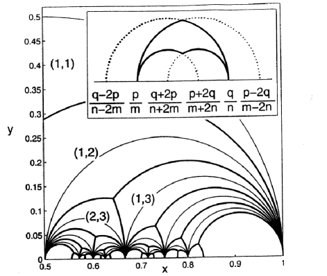
Figure 3: The $x,\,y$ plane partitioned by parastichy domains (thick lines). The domains are marked by parastichy pairs $(P_{1},P_{2})$. Only the $0.5<x<1$ region is shown, since the pattern is symmetric under $x\rightarrow x\pm 1,x\rightarrow 1-x$. Farey triangles are shown by thin lines (see Fig. 5).    Inset: A parastichy domain bounded by four semicircles (9).

Similar domains can be obtained for all combinations of $p$, $m$, $q$, and $n$, which satisfy the condition (7). These domains partition the $(x,y)$ plane as shown in Fig. 3. In this figure we display the parastichy domains only in the region $0.5<x<1$ because our partition of the plane is invariant under translations $x\to x+k$ and reflections $x\to k-x$. This invariance property accounts for the fact that the pairs $(x,y)$, $(x+1,y)$, and $(-x,y)$ represent the same lattice up to helicity change.

There is a useful relation of the plane partition by the parastichy domains $P_{1}=m$, $P_{2}=n$ and van Iterson diagram (Fig. 2). The boundaries of the parastichy domains correspond to rhombic lattices, because at the borderline where the parastichy pair changes the lattice must have next-shortest vectors of equal length. Therefore, the points where the domains join in three correspond to perfect triangular lattices (this property wil be discussed further in Sec. V.2). At the same time, these points are the triple branching points of van Iterson tree. Thus each branch of the tree resides within a single parastichy domain, connecting its opposite corners (compare Fig. 2 and Fig. 3). After associating each van Iterson branch with a parastichy domain we see that the parastichy numbers in van Iterson diagram are in fact identical to those introduced above using the plane partition. Therefore, each branch of van Iterson diagram is characterized by parastichy numbers $P_{1}$, $P_{2}$ which are constant within it and can change only at the branching of the tree.

It is interesting to understand the organization of the parastichy numbers $P_{1}$, $P_{2}$ throughout the $x,\,y$ plane in Fig. 3. Inspecting the parastichy pairs written in the adjacent domains shown Fig. 3 inset gives a simple addition rule: For a domain with $P_{1}=m$ and $P_{2}=n$, the two domains adjacent to it from below (closer to the $x$ axis) are lebeled by the pairs $P_{1}=m+n,\,P_{2}=n$ and $P_{1}=m,\,P_{2}=m+n$. As illustrated in Fig. 3, this relation between parastichy pairs of neighboring domains, so far conjectured empirically, describes organization of pairs $P_{1}$, $P_{2}$ in the entire $x,\,y$ plane. The addition rule for the numbers $P_{1}$, $P_{2}$ will be proven in Sec. IV.2.

For now taking the addition property for granted, we can infer that for any pair of mutually prime integers $m>0$ and $n>0$ a domain labeled by such a pair can be found in Fig. 3. It thus becomes evident that the pairs of consecutive Fibonacci numbers correspond to a very small sub-family of parastichy domains, while most of the domains are non-Fibonacci.

This observation helps to clarify that the cylindrical lattices realized in the natural world are a very small subset of all lattices that are mathematically possible, adding suspense to the problem of explaining the widespread occurrence of Fibonacci numbers. To help demystify it, in the next section additional ingredients will be added in the discussion: mechanical forces, energy and the development under stress.

IV The energy model

IV.1 Phyllotactic growth under stress: the sequence of deformations and adjustments

To describe interaction between different units of a phyllotactic pattern, we employ a repulsive potential $U({\bf r})$ of a generic form Levitov2 . In our model, this potential defines forces by which the points constituing the cylindrical lattice (1) repel each other. From a microscopic point of view, the interaction $U$ models the effects of rigidity of structural units and of contact pressure between them, as well as other similar effects arising at short distances (e.g. the volume constraint in dense packing of scales of a pine-tree cone). While the interactions of a short range or hard core type perhaps would be the most relevant for systems of interest, it is beneficial to allow for a generic repulsive interaction, since this helps to assess the robustness of phyllotactic growth.

Next, we introduce the interaction potential describing forces between the lattice points and define the energy functional. To that end, we will focus on the central force potential model, in which the force ${\bf F}=-\nabla U(r)$ points along the line connecting two interacting points. The potential $U(r)$ in this case is a function of the distance measured using the Euclidean metric in the plane obtained by unrolling the cylinder and the cylindrical lattice into 2D, as discussed above. To define the energy functional for a lattice we first note that the total energy obtained from all pairwise interactions, given by the expression

$$E_{\rm total}={1\over 2}\sum_{pmp^{\prime}m^{\prime}}U(|{\bf r}_{pm}-{\bf r}_{p^{\prime}m^{\prime}}|),$$ (10)

is formally divergent for an infinite lattice, either or a cylinder or in 2D. It is therefore more natural to consider the ‘energy density’ defined as energy per one lattice site. This quantity is given by

$$E(x,y)=\sum_{pm}U(r_{pm}),\quad r_{pm}=|{\bf r}_{pm}|,$$ (11)

where the sum runs over all vectors of the lattice (3). The quantity (11) is equal to the energy density per unit area times the unit cell area $A$. Hereafter we suppress the dependence on $A$, focusing mainly on the constant density case, $A=1$. We note parenthetically that the ${\bf r}=0$ term can be taken out from the sum (11) with no impact on the discussion. Indeed, this term corresponds to self-interaction, and thus eliminating it would merely change the energy by a constant which is independent of the lattice geometry and thus inessential for our analysis.

Below we will focus on the case of repulsive interactions, $dU(r)/dr<0$. In addition, for mathematical convenience, we assume that that $U(r)$ decays rapidly enough to assure convergence of the sum (11). The functional form of the interaction $U(r)$ can be taken, for example, as an expeonential $e^{-r/r_{0}}$, a gaussian $e^{-r^{2}/r_{0}^{2}}$, or a power law $r^{-\gamma}$. It will be clear from our discussion that the qualitative behavior is independent of the particular form of interaction.

One caveat associated with our definition of energy, Eq.(11), is that this quantity is defined as a sum over all lattice points (3), of which the points ${\bf r}=u{\bf i}+v{\bf j}$ with equal $v$ coordinates correspond to the same point of the spiral structure on the cylinder (1). Despite this, we treat these points as distinct in the sum over $i$ and $j$. Such a choice of the expression for the energy, Eq.(11), is deliberate: as we demonstrate below, the quantity (11) has hidden symmetries which underpin the robustness and universality of phyllotactic growth.

Further, one can argue that the approximation made in replacing the energy of a cylindrical lattice by that of a lattice in the two-dimensional plane is better than it sounds. Indeed, comparing the energy (11) to the energy of the cylindrical structure (1), with the interaction defined using the shortest distance on a cylinder, we note that the difference of the two energies corresponds to the part of the sum (11) with the $u$ component of the radius vector exceeding half of the cylinder circumference, $|u|>a/2$. However, as we will see below, the development under uniaxial stress makes the circumference $a$ increase so that already at a relatively early stage of growth it can exceed the range of interaction set by $U(r)$. As soon as this happened, the inaccuracy in the expression (11) becomes insignificant. This observation justifies using the expression (11) instead of a marginally more accurate but less symmetric expression for cylindrical lattices (1).

Next, we proceed to analyze the transformations of cylindrical lattice structures under stress. Increasing the pressure acting along the cylinder axis has two distinct effects. One is a compression of the system in the $z$-axis direction. Another is a buildup of pressure accompanied by a density change in the system. For simplicity, below we will treat these two effects as decoupled, assuming that the variation of stress does not affect pressure in the system, and hence the lattice density $\rho=A^{-1}$ is constant. This approximation is made on the grounds that the system compressibility depends mostly on the lattice average density and not as much on the details such as the angles between nearest-neighbor bonds and other geometric details LeeLevitov . We will therefore treat the distinction between the conditions of constant pressure and constant density as inessential, ignoring it in our discussion.

We implement the constant density approximation by describing the lattice defomration through changing the lattice parameter $y$ and, at the same time, maintaining constant $A$. As $y$ varies gradually from higher to smaller values, for each given $y$ value we have to adjust $x$ for the lattice energy to attain a local minimum,

$${\partial E\over\partial x}=0,\quad{\partial^{2}E\over\partial x^{2}}>0,\quad A,\,y=\text{const}$$ (12)

and then to examine the evolution of optimal $x$ as $y$ decreases from infinity to zero. The process (12) makes $x$ an implicit function of $y$. One can say that the function $x(y)$ describes the progression (or, “history”) of the deformation. That is, we assume that $y$ is controlled externally, and $x$ is a free parameter in which the system is trying to reach local equilibrium. The reason the roles of $x$ and $y$ are different becomes obvious from their geometric meaning: $y$ controls the spacing of lattice points along the cylinder axis, while $x$ corresponds to a lattice shear, or to a twist of the cylindrical structure (since $A$ is constant, neither $x$ nor $y$ affect the lattice density).

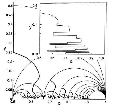
Figure 4: The dependence $x$ vs. $y$ (thick lines) for the local minima of the energy (10), describing cylindrical lattice (3) evolution under increasing uniaxial stress. The interaction $U(r)=e^{-5r}$ and unit density, $A=1$, was used in calculation. Farey triangles (Fig. 5) are shown to help exhibit the structure of the pattern (thin lines).    Inset: The trajectory of the global minimum of the energy (10) switches erratically between different branches of the local minima shown in the main panel.

The energy functional $E(x,y)$ governs the deformation and shear developing in the compressed lattice. The resulting trajectory in the lattice phase space $(x,y)$ can be linked to the behavior of the energy minima, Eq.(12). Namely, as the parameter $y$ is becoming smaller under uniaxial compression, the energy $E(x,y)$, taken at a fixed $y$ value, acquires more and more extremal points in $x$. In the phyllotaxis problem we are interested in tracing out the (local) minimum towards which the structure evolves without jumping to other minima. As we will see, it is instructive to analyse all local minima on equal footing. Such analysis will provide, in particular, an insight into the structure of the patterns resulting from the minima evolution under variation of $y$. This is exemplified in Fig. 4 where the trajectories for different energy minima obtained for the interaction $U(r)=e^{-5r}$ are shown. The resulting pattern of trajectories has a number of interesting properties:

1. For $y$ large enough there is only one energy minimum, located at $x=0.5$, which corresponds to the angle $\alpha$ in the generating spiral (1) equal to $180^{\text{o}}$. In terms of cylindrical lattices, $x=0.5$ describes the simplest imaginable structure in which all lattice points reside in one plane that cuts the cylinder vertically in two halves, the even-numbered and odd-numbered points located on the opposite sides of the cylinder in an alternating order.
   

2. At $y\approx 0.25$ this structure becomes unstable, and acquires a twist with a right-hand or left-hand helicity. The two opposite-helicity states are related by mirror symmetry, and thus have equal energies. At this $y$ value a single energy minimum transforms into a pair of adjacent minima. This is manifest in the $x=0.5$ trajectory splitting up at $y\approx 0.25$, and can be associated with a bifurcation of the evolving structure.
   

3. As $y$ is lowered further, trajectories in Fig. 4 display no other branching or bifurcation below the first bifurcation encountered at $y\approx 0.25$. This is despite the fact that many new energy minima appear as $y$ decreases, however each of these minima appears some distance away from the existing minima.
   

4. There are two principal trajectories that emerge at the bifurcation. Because of what has been said, the principal trajectories display smooth evolution below the bifurcation, displaying no secondary bifurcations. Hence, provided that the system evolution goes through the bifurcation point, at subsequent compression it will follow one of the two principal trajectories.

Of course, while the detailed behavior of the trajectories depends somewhat on the choice of the interaction $U(r)$, the general behavior of the minima appears to be robust. In particular, the properties 1,2,3,4 highlighted above are insensitive to the particular form of the interaction. This is exemplified, for instance, by the analysis in Refs. Levitov1 and  Levitov2 , which focusses on the interactions $U(r)=\exp(-r^{2})$ and $U(r)=-\ln r$, respectively.

Next we proceed to discuss what numbers of spirals, i.e. the parasticy numbers, can be realized for the structures obtained for different trajectories. This can be analyzed most easily by superimposing the trajectories with the parastichy domains constructed above in Sec.III.2 After superimposing the trajectories with the domains in Fig.3, one makes a striking observation that the principal trajectory, following the bifurcation, passes exclusively through the Fibonacci domains. This result means that, starting from the simplest structure, the system does not have any other choice but to evolve into a Fibonacci structure. The system, responding to $y$ gradually varying by maintaining local equilibrium in $x$, is driven through the Fibonacci sequence of states. This is so because in order to switch to a non-Fibonacci state it has to overcome a finite energy barrier.

We note that in our approach to modeling phyllotaxis by a requirement that the system traces local energy minima the word “local” is absolutely crucial. If instead one would have chosen to analyze the global energy minimum, for each $y$ seeking the $x$ value yielding the lowest energy state, the result would have been quite different. This is illustrated in the inset of Fig. 4 which shows the position of the global minimum which jumps in a perfectly erratic way between the principal and non-principal trajectories. Such jumping trajectory shows no regularity whatsoever, in particular it passes through many non-Fibonacci parastichy domains and generates structures of a mostly non-Fibonacci type. This obviously means that the global energy criterion, while being useful in a variety of other problems, does not provide a good guidance in the phyllotaxis problem. One might argue that this is in a sense natural since the phyllotactic systems of interest, which develop into Fibonacci structures, are macroscopic even at an early stage of growth. Indeed, even an embryo at an early developmental stage is a macroscopic object which is unlikely to transcend structural barriers due to thermal or environmental fluctuations, even if that would take it to a lower energy state. This is obviously related to the fact that for a macroscopic system the time required for reaching the lowest energy state by jumping over barriers would be very large, presumably much larger than the growth time. We therefore conclude that, while local energy minimization has a clear physical significance in describing growth, the models based on a global energy minimization, which are blind to the presence of barriers, are of limited utility.

Returning to the discussion of diffrent trajectories in Fig. 4, it is intresting to note that the next principal trajectory in Fig. 4 generates structures from the Lucas sequence 1, 3, 4, 7, 11, 18, etc. This is in good agreement with (and provides an explanation for) the well known fact that the Lucas numbers are the most common exception in phyllotaxis. To obtain these numbers through our mechanical development model one simply has to assume that the system makes one mistake at the very beginning by jumping over the energy barrier to the lattice in the $(3,1)$ domain, after which it strictly follows the rules of the game. One can crudely estimate the barrier height, and see that it increases inversely with $y$. This implies that a mistake, if happened at all, would be most likely to occur at higher $y$ values, i.e. at the beginning of the growth. In other words, the Lucas sequence is associated with the mistake in the growth which is the most likely one to occur.

We verified, by performing numerical simulations and otherwise, that the results described above show considerable robustness and are not interaction-specific. Namely, we find that all ‘reasonable’ repulsive interactions, $dU/dr<0$, fit the bill. One might argue that a particular form of the repulsive interaction would not matter as long as it renders the lattice stable. This conjecture is indeed true, as will be discussed in the next section where we show that the energy model can be treated analytically and rigorously. After describing the rigorous results, we will return to the robustness property and formulate more precisely the conditions on the potential under which the energy model leads to Fibonacci structures. The robustness property provides a lot of freedom in varying the form of interaction. Furthermore, one can generalize the results to the interactions that vary during the growth (see Sec. VI.1), which provides insight into phyllotactic growth in the geometries other than cyclindrical (see Sec. VI.2).

Finally, we make a cautionary remark that using the degree of compression $y$ as a control parameter may not be entirely physical. In a real system, the external forces producing stresses in a growing system correspond to pressure and strain, with the resulting deformation governed by the conditions of mechanical stability. However, it can be shown LeeLevitov that in our problem the stress and the deformation are in a one-to-one relation, and so, to avoid unnecessary complications, in what follows we will replace the actual external forces by the quantity $y$ defined above, which will act as a control parameter .

IV.2 Symmetries of the energy

In this section we will discuss the symmetry properties of the energy function, Eq.(11), focusing on the topography defined by $E(x,y,A)$ in the $x-y$ plane. As we will see, the behavior of $E(x,y,A)$ is rather peculiar: there are infinitely many energy minima which are all degenerate, i.e. correspond to identical energy values. Furthermore, the $E(x,y,A)$ topography is such that the minima are organized in an intricate network resembling a mountain range with a system of valleys surrounded by peaks and passes. To understand the resulting structure, we will introduce a group of modular symmetries, comprised of the transformations of the $x-y$ plane that leave the function $E(x,y,A)$ invariant. We will choose the fundamental domain of the symmetry group and define the corresponding partition of the $x-y$ plane such that it elucidates the network induced by the $E(x,y,A)$ topography. As we will see, this construction greatly facilitates the analysis and leads to a simple explanation of the pattern of the growth trajectories, such as that in Fig. 4. In subsequent sections the modular symmetry will be used to treat the problem analytically and rigorously, and to prove the stability of Fibonacci structures in a rather general way.

To make our discussion of modular symmetry more transparent, it will be convenient to introduce the complex variable $z=x+iy$ and view the $(x,y)$ plane as a complex $z$ plane. The energy function $E(x,y,A)$ will then be defined on the so-called modular space, allowing our analysis to benefit from a high symmetry revealed by such a construction. Accordingly, we will use the notation $E(z,A)$ instead of $E(x,y,A)$.

Furthermore, it is also convenient to use complex parameterization for the ‘physical space’ (the unfolded cylinder) where the lattices (3), obtained by unrolling cylindrical lattices, are defined. In passing to the complex notation we identify ${\bf i}\to 1$, ${\bf j}\to i$, after which Eq.(3) reads

$$r_{pm}(z)=u_{pm}(z)+iv_{pm}(z)=\sqrt{A\over{\rm Im}(z)}\ (p-m\overline{z})\ ,$$ (13)

where $\overline{z}=x-iy$.

General modular transformations of a complex plane are defined in a standard way as fractional linear transformations of a complex variable. These trasformations and the associated mappings of the complex plane are often encountered in the complex-variable calculus and its applications Apostol . In particular, these transformations play an important role in the hyperbolic geometry. This relation, as will become clear shortly, will be pivotal for our discussion.

Integer modular transformations of a complex variable Apostol are defined by using a unimodular $2\times 2$ matrix with integer elements,

$${\bf A}=\left(\begin{array}[]{cc}a&b\\ c&d\end{array}\right),\quad|\mbox{ det }{\bf A}|=1\ .$$ (14)

Then the corresponding modular transformations of $z$ are defined as

$$z\rightarrow z^{\prime} = (az+b)/(cz+d),\quad\mbox{if\ \ det }{\bf A}=1,$$

$$z\rightarrow z^{\prime} = (a\overline{z}+b)/(c\overline{z}+d),\quad\mbox{if\ \ det }{\bf A}=-1\ .$$ (15)

Separate definitions for the two signs of the determinant $\text{det}{\bf A}$ are required to assure that the halfplane $\mbox{ Im }z^{\prime}>0$ remains invariant under these transformations. The transformations in Eq.(IV.2) define an analytic function for $\text{det}\,{\bf A}=1$, and an anti-analytic function for $\text{det}\,{\bf A}=-1$.

It is easily verified that the transformations in Eq.(IV.2) form a group, with the group multiplication represented by matrix multiplication. Namely, the composition of two modular transformations $z\to z^{\prime}\to z^{\prime\prime}$ is a modular transformation associated with a matrix ${\bf A^{\prime}A}$, where ${\bf A}$ and ${\bf A}$ describe the transformations $z\to z^{\prime}$ and $z^{\prime}\to z^{\prime\prime}$, respectively.

In group theory, the $2\times 2$ integer matrices with a unit determinant and a group multiplication defined through matrix multiplication is known as the group $SL(2,Z)$. Here we are interested in a bigger group known as $GL(2,Z)$ comprised of integer matrices with the determinant $+1$ or $-1$ which contains the group $SL(2,Z)$ as a subgroup, $GL(2,Z)/SL(2,Z)=Z_{2}$.

The significance of these transformations is elucidated by the following

Theorem: The energy $E(z,A)$ is invariant under any modular transformation (IV.2).

Proof: As a first step, we show that under the transformations of $z$ given in Eq.(IV.2) the lattices (13) change in avery simple way. Namely, these transformations define Euclidean rotations of the lattice, when $\mbox{ det }{\bf A}$=1, and a rotation combined with a mirror reflection, when $\mbox{ det }{\bf A}=-1$.

Indeed, by a direct calculation one verifies that the lattice (13) changes under the transformations (IV.2) as follows:

$$r_{pm}(z) = e^{i\phi}r_{p^{\prime}m^{\prime}}(z^{\prime})\quad\mbox{for\quad det }{\bf A}=1,$$

$$r_{pm}(z) = e^{i\phi}\overline{r_{p^{\prime}m^{\prime}}(z^{\prime})}\quad\mbox{for\quad det }{\bf A}=-1,$$ (16)

where $p^{\prime}$, $m^{\prime}$ and the rotation angle $\phi$ are defined by

$$p^{\prime}=ap+bm,\quad m^{\prime}=cp+dm,$$

$$\exp(2i\phi)=(c\overline{z}+d)/(cz+d).$$ (17)

Eq.(16) means that the lattices (13), under the transformations (IV.2), are mapped to isometric lattices.

Next, to complete the proof, we note that the lattice energy $E(z,A)$, Eq.(11), is given in terms of an isotropic, angle-independent interaction $U(r)$. As a result, the quantity $E(z,A)$ is invariant under distance-preserving transformations of the lattice, such as the rotations and mirror-reflections in Eq.(16).
QED

Symmetry can be used to gain insight into the properties of energy $E(z,A)$ in a much the same way as, for example, periodic functions are analyzed by studying them within the fundamental period of the translation symmetry group and then using the periodicity property to extend the function to the entire space. To apply this strategy we need to identify a suitable tesselation of the complex $z$ plane induced by the $GL(2,Z)$ symmetry. This tesselation will play a role in our analysis analogous to periodic tesselations of space used for describing the structure of periodic functions.

An appropriate group-theoretic vehicle used to characterize functions invariant under some symmetry group is that of a fundamental domain. The fundamental domain is defined a geometric shape in the space of the action of the group such that its images obtained by applying all group elements cover the whole space with no gaps and no overlaps (except, possibly, over boundaries). Loosely speaking, the fundamental domain is a minimal space region that, after having been replicated by the group transformations, partitions the entire space.

For the symmetry group (IV.2), we need a domain in the $z$ plane chosen so that the mappings (IV.2) of the domain cover the $z$ plane, overlapping only along boundaries. The fundamental domain construction for the modular group, introduced by Gauss, is widely discussed in mathematical literature. (For example, see Ref. Apostol , Chap. 2, and Ref. hyperbolicgeometry , Chap. 5.) However, the standard Gaussian fundamental domain known as the “modular figure” will not be that useful, because for our purpose it is too small. Instead, we will use a 3 times larger domain, which is not a truly fundamental domain in the sense of the standard definition. We will see below that the larger domain is more natural from the point of view of the energy topography in the $z$ plane. The relation of our domain to the Gaussian domain will be discussed in Sec. V.2.

Let us begin with introducing in the halfplane ${\rm Im}\,z\geq 0$ a family of semicircles:

$$y=\sqrt{\left(x-{p\over m}\right)\left({q\over n}-x\right)}\ ,\ {p\over m}\leq x\leq{q\over n}\ ,\$$ (18)

where $p$, $m$, $q$, and $n$ are integers with $pn-mq=\pm 1$ and $m>0$, $n>0$. (In Figs. 3, 4 the semicircles are shown by thin lines.) We will denote each semicircle by its end points: $[p/m,q/n]$. It is convenient to allow formally the combinations in which either $m$ or $n$ is zero, by adding vertical straight lines $x=q$. (It follows from $pn-mq=\pm 1$ that if $m=0$, then $n=1$.) Our notation for such “generalized semicircles” that connect $x=q$ with $x=\infty$, will be $[1/0,q/1]$.

It turns out that two semicircles of this family can intersect only at the real axis, at the point where they are tangent. By virtue of this property, the semicircles divide the $x-y$ plane into curvilinear triangles with the vertices on the $x$ axis at the points $x=p/m,\ q/n,\ r/s$, where $r=p+q$, $s=m+n$. We will denote such triangles by specifying the $x$-coordinate of their vertices: $[p/m,q/n,(p+q)/(m+n)]$. These triangles are called Farey triangles, and are closely related to the so called Farey numbers. Farey triangles and Farey numbers constitute a nice subject on the borderline between arithmetic and elementary geometry, and are well accounted in mathematical literature (see, e.g., the textbooks Apostol ; hyperbolicgeometry .)

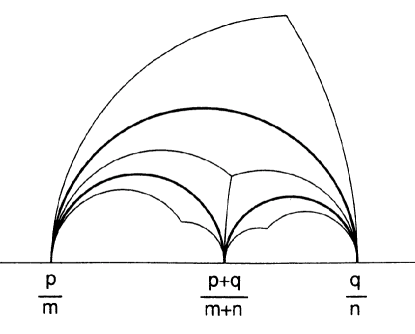
Figure 5: Relation between the Farey triangles (Fig. 3, thick lines) and parastichy domains (Figs. 3,4, thin lines), which partition the complex $z$ plane in two different ways, is illustrated. Each Farey triangle is centered at a corner of three adjacent parastichy domains. Each parastichy domain ovelaps with two adjacent Farey triangles.

In the number theory, Farey numbers is a name for a construction that organizes all rational numbers $0\leq p/m\leq 1$ in a hierarchy. Starting with $0=0/1$ and $1=1/1$, one applies the Farey sum rule, $p/m\oplus q/n=(p+q)/(m+n)$, and successively generates more and more rational numbers (see Apostol , Chap.5). The order in which the numbers are generated coincides with the hierarchy of our Farey triangles: one vertex of each triangle is Farey sum of two other vertices (see Fig. 5).

Let us comment on the relation between the Farey triangles and the parastichy domains. Both partitions of the $z$ plane are invariant under modular transformations. Comparing Eq. 18 with the parastichy domains construction of Sec. III.2, it is obvious that for a given Farey triangle $[p/m,q/n,(p+q)/(m+n)]$, the sides $[p/m,q/n]$, $[p/m,(p+q)/(m+n)]$, and $[q/n,(p+q)/(m+n)]$ belong to the parastichy domains with the parastichy pairs $(m,n)$, $(m,m+n)$, and $(n,m+n)$, respectively (see Eq. 9 and Fig. 5). Hence, each Farey triangle overlaps with three parastichy domains, one side per one domain, and conversely, each parastichy domain overlaps with two Farey triangles. The relation of the two ways of partitioning the $z$ plane will be studied in more detail in Sec. V, and then used for the discussion of the stability of Fibonacci numbers.

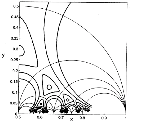
Figure 6: A contour plot (thick lines) of the lattice energy for the interaction $U(r)=\exp(-5r)$. Farey triangles (thin lines) are shown for guidance. The contours behavior in all Farey triangles is similar.

To see the role of Farey triangles, in Fig. 6 we draw a contour plot of the energy for the potential $U(r)=e^{-5r}$, together with the Farey triangles partitioning the $z$ plane. It is evident from the figure that the energy contours display similar behavior in each triangle. Qualitatively, from the topography point of view, there is a “valley” inside each Farey triangle, with a minimum at the center. For each valley there are three neighboring valleys in the adjacent triangles, “connected” with it by “passes” through the saddles located at the middle of each side of the Farey triangles. At the corners of the triangle there are peaks of infinite height.

Schematically, the valleys in Fig. 6 are connected with the neighboring valleys in a structure that can be characterized as a Cayley tree with a branching number three. This tree can be compared to the pattern of trajectories in Fig. 4 obtained by looking at the energy minima in $x$ at fixed $y$. Obviously, no matter what $y$, the minima will reside somewhere within the valleys, away from the peaks. Therefore, when $y$ varies continuously, the minima trace out the valleys and their interconnections. Comparing Fig. 4 to Fig. 6, it is evident that the pattern of the minima approximately repeats the pattern of the valleys. From a topological point of view, the branching points of the Cayley tree of valleys correspond to quasibranching of the minima trajectories that one defines by bridging different trajectories across the gaps Levitov2 . As $y$ varies, each trajectory explores a sequence of neighboring valleys, and quasibranchings manifest that there are three neighboring valleys around each valley.

However, let us emphasize that the trajectories of minima in Fig. 4 are not invariant under the modular transformations. Technically speaking, the reason is that we are looking for minima of a modular symmetric function $E(z,A)$ under a non-symmetric constraint: $y={\rm const}$. Obviously, if the pattern of minima were symmetric, all parastichy pairs would be equally likely to appear. Hence, the absence of symmetry is an ultimate cause of the appearance of Fibonacci numbers.

It is important to realize that the problem has incomplete symmetry: the lattice energy is modular-symmetric, but the deformation process is not. Thus a concept of asymmetry emerges, which implies the absence of symmetry, but nevertheless certain closeness to an exact symmetry. We will see that the asymmetry is a much more powerful notion than just total absence of symmetry. The modular symmetry transformations enable one to compare the energy minima trajectories in different Farey triangles. It is even correct to say that the problem of stability of Fibonacci numbers in phyllotaxis is now reduced to the analysis of the asymmetry of the pattern of energy minima trajectories. This idea will be the bottom line of the following discussion.

V Universality of Fibonacci numbers

V.1 Plan of the discussion

In this section we will prove a rather general statement about any energy minima trajectory. Although, strictly speaking, we are interested only in the principal trajectory (which is Fibonacci), there is a lot of advantage in considering all trajectories together.

To formulate our main result, let us recall that a generalized Fibonacci sequence is a sequence of integers $\Phi_{n}$ obeying the Fibonacci recursion relation,

$$\Phi_{n+1}=\Phi_{n}+\Phi_{n-1},$$ (19)

where the starting numbers $\Phi_{0}$, $\Phi_{1}$ can be any integers. For example, the standard Fibonacci sequence and the Lucas sequence are given by $\Phi_{0}=1,\,\Phi_{1}=1$ and $\Phi_{0}=1,\,\Phi_{1}=3$, respectively.

Main theorem: For any interaction $U(r)$ from the family defined below, a continuous trajectory of the energy minima in the $z$ plane goes through the sequence of parastichy domains with the parastichy pairs from a generalized Fibonacci sequence. The first two numbers of the sequence are determined by the beginning of the trajectory.

Once the theorem is proven, the result about having only Fibonacci numbers on the principal trajectory follows from the fact that it begins in the $(1,1)$ parastichy domain.

It is worth remarking that in the theorem the word “continuous” is crucial! Given that the deformation of the lattice is continuous, the theorem states that the deformation stages all are (generalized) Fibonacci. On the other hand, if the deformation makes the lattice unstable, and it abruptly transforms to some other structure or lattice, with a jump on the $z$ plane, the theorem is not claiming anything.

The class of potentials $U(r)$ for which the theorem holds is defined by the following two conditions.
a) The deformation is a continuous process, and does not make the lattice unstable.
b) The topography of the energy $E(z)$ is the simplest required by modular symmetry: no critical points other than the $\triangle$ and $\Box$ points (see Fig. 6 and Sec. V.2).
Condition a) is stated in the theorem, and the role and meaning of condition b) will become evident in the proof (see Sec. V.3). The conditions a) and b) define implicitly a large family of interactions, apparently including all repulsive potentials. At the moment, however, an explicit characterization of this family is lacking. (Maybe it is worthwhile to mention that we failed to find exceptions among repulsive interactions.)

The proof of the theorem relies on the modular symmetry of the energy $E(z)$ (see Sec. IV.2), which gives the topography of $E(z)$ in the entire $z$ plane from that within a single Farey triangle. Also, we will use the relation between Farey triangles and parastichy domains, already mentioned in Sec. III.2. We will discuss it again and summarize in Sec. V.2. The plan of the proof includes the following two steps. First, by making use of the modular symmetry, we replace the global statement about the trajectories behavior in the entire $z$ plane by an equivalent local statement about the behavior in a single Farey triangle (see Lemmas 1, 2, 3 in Sec. V.3). Then, by using modular symmetries, we treat a minima trajectory within a single Farey triangle, and find the relation with the parastichy domains. For that, we map the lines $y={\rm const}$ in an arbitrary Farey triangle onto a certain family of curves in a “reference” Farey triangle, and then (locally) minimize the energy on these curves. At this step, we establish a Fibonacci type relation between the parastichy domains traced by a trajectory.

Loosely speaking, the Farey triangles play an “organizing role” in the $z$ plane. They represent something like standard blocks, or units for the trajectories. In some sense, the behavior of trajectories inside all triangles is similar, and the topology of the trajectories pattern can be constructed by replicating one triangle with the modular symmetries.

V.2 Modular symmetry and Farey triangles

Here we review basic facts about Farey triangles on the hyperbolic plane, and study the relation of the Farey triangles and parastichy domains. Necessarily, our discussion be brief. (We refer interested reader to very good texts by Apostol Apostol and Iversen hyperbolicgeometry .)

The geometric role of modular transformations is that they preserve the hyperbolic metric $dl^{2}=|{\rm Im}\,z|^{-2}d\bar{z}dz$. The ${\rm Im}\,z\,\geq\,0$ halfplane supplied with this metric is called the hyperbolic plane. The transformations that preserve the hyperbolic metric (they are called isometries) form a group known as $PSL_{2}(R)$ or $SL_{2}(R)\otimes Z_{2}$, that plays a role in the hyperbolic geometry similar to that of space translations and rotations in the Euclidean geometry. All hyperbolic isometries have the form (IV.2) with arbitrary real $a$, $b$, $c$, and $d$, such that ${\rm det}{\bf A}=\pm 1$. The modular transformations (IV.2) with integer $a$, $b$, $c$, $d$, and ${\rm det}{\bf A}=\pm 1$, form an infinite discrete subgroup of the group of all isometries, as, for instance, symmetries of a crystal in the Euclidean space do. The group theory notation for the modular group is $PSL_{2}(Z)$ or $SL_{2}(Z)\otimes Z_{2}$.

The geodesics hyperbolicgeometry of the hyperbolic metric are semicircles with the diameters on the real axis:

$$y=\sqrt{\left(x-x_{0}\right)\left(x_{1}-x\right)}\ ,\ \ x_{0}<x<x_{1}\ .$$ (20)

Obviously, the isometries (IV.2) map any geodesic to a geodesic. There are two different classes of hyperbolic isometries:
a) The mappings with ${\rm det}{\bf A}=+1$ that have just two fixed points on the real axis;
b) The mappings with ${\rm det}{\bf A}=-1$ that have a whole geodesic of fixed points.
Given a geodesic (20), the mapping that leaves it fixed is given implicitly by

$${z^{\prime}-x_{0}\over z^{\prime}-x_{1}}=-{\bar{z}-x_{0}\over\bar{z}-x_{1}}\ .$$ (21)

Such a transformation is analogous to a Euclidean reflection, with the geodesic (20) corresponding to a mirror. A composition of an even number of transformations of the type b) is a transformation of the type a).

The property of Farey triangles that makes them useful is that the modular transformations (IV.2) map any Farey triangle either onto another Farey triangle, or onto itself. To see why is that, one first notes that by a transformation (IV.2) with unrestricted $a$, $b$, $c$, and $d$, we can map any three points on the real axis onto any other three points (because it is a fractional-linear function). Then one checks that, since vertices of Farey triangles are rationals, the numbers $a$, $b$, $c$, and $d$ can be chosen to be integer, with ${\rm det}{\bf A}=\pm 1$. This follows from the explicit form of the transformation (IV.2) that maps an (arbitrary) Farey triangle $[p/m,q/n,(p+q)/(m+n)]$ onto the triangle $[0/1,1/1,1/2]$:

$${\bf A}=\left(\begin{array}[]{cc}m&-p\\ m-n&-p+q\end{array}\right)\ .$$ (22)

Applied to the lattice energy $E(z)$, modular symmetries relate the values of $E$ at different points of the $z$ plane. Given $E(z)$ inside one Farey triangle, the modular transformations extend it throughout the whole plane. However, let us emphasize that the function $E(z)$ within one Farey triangle has certain symmetry properties, and hence it is not completely arbitrary. The reason is that, as it was mentioned above, the Farey triangles are larger than the actual fundamental domains of the modular group. For each triangle there are six modular transformations (including the indentity) that map it onto itself. The energy $E(z)$ is invariant under these transformations, and hence there is a usual relation between the symmetries of a triangle and the behavior of the function $E(z)$ inside it:
a) There are extremal points of $E(z)$ at all symmetry points of the triangle transformations;
b) The contours of $E(z)$ are normal to the invariant lines of the transformations.
Since the topography of the energy $E(z)$ within a Farey triangle will be crucial for our discussion, let us describe here the triangle symmetries in some detail.

There is a total of six modular transformations which map a Farey triangle onto itself. From the group theory point of view, the symmetry group of a Farey triangle is identical to that of an equilateral triangle in a Euclidean plane that includes three reflections, two rotations, and the identity. Each permutation of the triangle vertices defines a modular transformation (since it is a fractional-linear transformation). For example, the transformation of the triangle $[p/m,q/n,(p+q)/(m+n)]$ that interchanges $p/m$ with $q/n$, and preserves $(p+q)/(m+n)$, is a reflection (21) with respect to the geodesic $[(p+q)/(m+n),(p-q)/(m-n)]$. The two other reflections correspond to the geodesics $[p/m,(p+2q)/(m+2n)]$ and $[q/n,(2p+q)/(2m+n)]$. Like in the Euclidean plane, where a composition of two reflections is a rotation, for the Farey triangle the composition of two reflections is a transformation giving rise to a cyclic permutation of the vertices. The intersection of the three geodesics

$$z = {pm+qn+pn/2+mq/2\over m^{2}+mn+n^{2}}$$

$$+\ i\ {\sqrt{3}\over 2}{1\over m^{2}+mn+n^{2}}.$$

is a symmetry point of the triangle invariant under all six symmetries of the triangle.

The symmetry lines of the Farey triangle are the three geodesics listed above, and also the three sides of the triangle, $[p/m,q/n]$, $[p/m,(p+q)/(m+n)]$, and $[q/n,(p+q)/(m+n)]$, since the reflections (21) about them are modular transformations that map the triangle $[p/m,q/n,(p+q)/(m+n)]$ to the three adjacent triangles. There are three symmetry points on the sides of the triangle given by the intersections of the symmetry lines. For example, the side $[p/m,q/n]$ intersects with $[(p+q)/(m+n),(p-q)/(m-n)]$ at

$$z={pm+qn\over m^{2}+n^{2}}+i{1\over m^{2}+n^{2}}.$$ (24)

The symmetry lines and the points (V.2) and (24) have a simple meaning in terms of the geometry of the lattice (3). The Farey triangle sides correspond to the lattices with a rectangular unit cell. The geodesics $[(p+q)/(m+n),(p-q)/(m-n)]$, $[p/m,(p+2q)/(m+2n)]$, and $[q/n,(2p+q)/(2m+n)]$ correspond to the lattices with a rhombic unit cell. One verifies this immediately by checking that the conditions ${\bf r}_{pm}\cdot{\bf r}_{qn}=0$, and $|{\bf r}_{pm}|=|{\bf r}_{qn}|$ define the geodesics $[p/m,q/n]$, and $[(p-q)/(m-n),(p+q)/(m+n)]$, respectively. Consequently, the points of the form (V.2) correspond to perfect triangular lattices, and the points (24) correspond to square lattices. We will call them $\triangle$ points and $\Box$ points, respectively. Each Farey triangle contains one $\triangle$ point in its interior and three $\Box$ points, one per each side.

The parastichy domains, as we found in Sec. III.2, are defined by the lines corresponding to rhombic lattices, i.e., by the symmetry lines. The corners of the parastichy domains are the $\triangle$ points. The boundaries are the portions of the symmetry lines extending from the $\triangle$ point to the Farey triangle vertices. At each $\triangle$ point three parastichy domains are adjacent. The parastichy pairs of the three parastichy domains overlapping with a Farey triangle $[p/m,q/n,(p+q)/(m+n)]$ are $(m,n)$, $(m,m+n)$, and $(n,m+n)$.

The symmetry points (V.2) and (24) are extremal points of the energy $E(z)$. At the $\triangle$ points the energy must have local minimum, since a perfect triangular lattice is a lowest energy configuration for an isotropic repulsive interaction. The minima at the centers of the valleys inside the Farey triangles in Fig. 6 are at the $\triangle$ points. At the corners of the Farey triangles the energy is maximal, since at these points one of the lattice periods vanishes, and the energy diverges. Given that the maxima are at the corners, and the minima at the centers, the $\Box$ points have to be the saddle points. (The square lattice has higher energy than the triangular lattice, and it is unstable with respect to a deformation towards triangular lattice through a continuous sequence of rhombic lattices.) Such a configuration of extremal points, located only at the symmetry points, is a minimal combination required by symmetry. For an arbitrary interaction, in principle, one could have other extremal points of the energy, not associated with the symmetry points of the Farey triangles. However, that would make the discussion unnecessarily complicated, and moreover, for typical simple repulsive interactions (exponential, gaussian, power law, etc) there are no additional extremal points. Therefore, in the following discussion we will assume that there are no other extremal points besides those required by symmetry.

Another useful property is that, by symmetry, the contours of the energy $E(z)$ are normal to the Farey triangle sides and the symmetry lines, everywhere except the $\Box$ and $\triangle$ points. This result will be crucial in the following discussion.

V.3 Farey partition of the hyperbolic plane and the trajectories of energy minima

To prove the main theorem, we have to see why the whole infinite sequence of the parastichy domains traced by an energy minima trajectory has the parastichy pairs that obey the Fibonacci addition rule. For that we will study the relation between the Farey triangles and the minima trajectories. The theorem statement is global, since it states the trajectories behavior in the entire $z$ plane. Our first step will be to replace it by local statements which are equivalent to the theorem, but talk only about one Farey triangle. One can say that we reduce the mystery all over the $z$ plane to the mystery inside one Farey triangle. The following three Lemmas together are equivalent to the statement of the main theorem.

Lemma 1  The minima trajectories enter or leave Farey triangles only through the $\Box$ points.

Lemma 2  The trajectories enter or leave the parastichy domains only through the $\triangle$ points. Any $\triangle$ point belongs to one of the trajectories.

Lemma 3  At a $\triangle$ point, by going from one to another parastichy domain the trajectory obeys the Fibonacci rule: after exiting the domain $(m,n)$, $m<n$, it enters the domain $(n,m+n)$.

Given the starting point of a continuous trajectory of minima, the three Lemmas completely determine through which sequence of Farey triangles and parastichy domains the trajectory proceeds. The Lemmas 1, 2 state that, no matter what interaction, there are $\Box$ and $\triangle$ points on each trajectory. Although the trajectory may be sensitive to the interaction, the sequence of the $\Box$ and $\triangle$ points through which it goes is decided purely geometrically, and does not depend on the interaction.

As for the $\triangle$ points, since perfect triangular lattice has lowest energy, it is understandable that the $\triangle$ points always lie on trajectories. However, the fact that (some) $\Box$ points also lie on the trajectories comes as a surprise. We will see that both Lemma 1 and 2 follow from the modular symmetry.

Lemma 3 states that the behavior of trajectories near the $\triangle$ points determines the evolution of parastichy pairs. Each $\triangle$ is a corner of three parastichy domains (say, with the pairs $(m,n)$, $(m,m+n)$, and $(n,m+n)$). The rule that the change of the pair is always $(m,n)\rightarrow(n,m+n)$, where $m<n$, applied iteratively along the trajectory, evidently leads to a generalized Fibonacci sequence. According to Lemma 3, there is no trajectory branching: new trajectory in the parastichy domain $(m,m+n)$, $m<n$, emerges at a finite distance from the $\triangle$ point.

Note that Lemma 3 is not applicable to the triangle $[0/1,1/1,1/2]$, ($m=n=1$), where branching occurs at the bifurcation point.

Proof:     To prove the lemmas for a given Farey triangle (say $[p/m,q/n,(p+q)/(m+n)]$, $m<n$) we use modular symmetry (22), and map this triangle onto $[0/1,1/1,1/2]$. To study how the energy minima at constant $y$ transform under this mapping, we have to find out how the constraint $y={\rm const}$ transforms. Under the transformation (22), the family of lines $y=\lambda$ is mapped to a family of circles tangent to the real axis,

$$|z-(x_{0}+iy_{0})|^{2}=y_{0}^{2},$$ (25)

where $x_{0}=m/(m-n)$, and $y_{0}=1/(2(m-n)^{2}\lambda)$. The images of the minima can be found by (locally) minimizing the energy on the circles (25).

This task is greatly facilitated by the following variable change,

$$z\rightarrow w=(-i\sqrt{3}\overline{z}+\epsilon)/(i\sqrt{3}\overline{z}+\overline{\epsilon}),$$ (26)

where $\epsilon=e^{i\pi/3}=1/2+i\sqrt{3}/2$. It maps the upper $z$ plane onto a unit circle $|w|=1$. Fig. 7a shows the contours of the energy taken as a function of $w$.

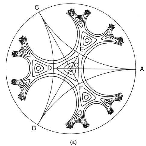
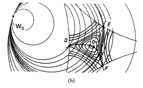
Figure 7: (a) A contour plot (thick lines) of the lattice energy for the interaction $U(r)=\exp(-5r)$, mapped to the $w$ plane by (26). The triangle $[C,B,A]$ is a mapping of the Farey triangle $[0/1,1/1,1/2]$. (b) A trajectory of energy minimum enters the triangle $[A,B,C]$ through the point $D$, and passes the point $O$ to exit through the point $F$. A new trajectory is created near the point $E$, and exits through the point $E$.

Under the variable change (26), the Farey triangle $[0/1,1/1,1/2]$ maps onto the triangle $[\epsilon^{2},\overline{\epsilon}^{2},1]=[C,B,A]$. The $\triangle$ point maps to the point $O$ and the three $\Box$ points map to the points $D$, $E$, and $F$. The parastichy boundaries map onto the lines $OA$, $OB$, and $OC$. The curved triangles $AOB$, $BOC$, $COA$ belong to parastichy domains $(n,m+n)$, $(m,n)$, and $(m,m+n)$, respectively.

The family of circles in Eq. 25 maps to a new family of circles

$$|w-w_{0}(1-r)|=r,$$

$$w_{0}=(m-(m+n)\epsilon)/(m-(m+n)\overline{\epsilon}),$$ (27)

$$r=\sqrt{3}/\left(\sqrt{3}+2\lambda\left(m^{2}+mn+n^{2}\right)\right).$$

which are tangent to the unit circle at $w_{0}$. We compute

$${\rm arg}(w_{0})=2\,\arctan\left(n+m)/(n-m)\right),$$ (28)

and find $2\pi/3<\mbox{arg}(w_{0})\leq\pi$, since $0\leq m\leq n$.

The behavior of the energy contours within the triangle $[A,B,C]$ follows from the results of Sec. V. The contours are smooth curves everywhere except the extremal points: $A$, $B$, $C$, $D$, $E$, $F$, and $O$. Also, according to the last statement of Sec. V, the contours are everywhere perpendicular to the arcs $AB$, $BC$, $CA$, and to the segments $AD$, $BE$, $CF$.

Now we are ready to study the trajectories. Geometrically, the trajectories points are those where the contours are tangent to the circles (27). It is simple to see that the circles (27) cannot be perpendicular to $AB$, $BC$, $CA$, $AD$, $BE$, $CF$, provided that $\mbox{arg}(w_{0})\neq\pi$. But $\mbox{arg}(w_{0})=\pi$ can occur only for the special case $m=1$, $n=1$, excluded by the condition $m<n$. Thus, we proved Lemma 1 and Lemma 2.

Modular symmetry implies that in the vicinity of the $\triangle$ point $O$ the contours are circles. From that, it follows that at the point $O$ the trajectory is tangent to the straight line joining $O$ and $w_{0}$ (Fig. 7(b)), and also that the trajectory branching does not happen. Since $2\pi/3<\mbox{arg}(w_{0})<\pi$, the trajectory in $BOC$ passes $O$ to enter $AOB$. Recalling that parastichy pairs in $BOC$ and $AOB$ are $(m,n)$ and $(n,m+n)$, respectively, one gets the Fibonacci rule, thus proving Lemma 3. QED

Finally, let us discuss the case $m=1$, $n=1$, in which Lemma 3 does not hold. However, if the method of the proof is applied to this case, it yields $\mbox{arg}(w_{0})=\pi$, that is a family of circles (27) perpendicular to $AD$. Then, obviously Lemma 1 is still valid, since the circles cannot be perpendicular to $AB$, $BC$, $CA$. The trajectory goes along the segment $AD$ up to some point within the segment $AO$, where the bifurcation occurs. At this point, the trajectory gives rise to a pair of symmetric principal trajectories, which reflects the $x\rightarrow 1-x$ symmetry. Thereafter, the principal trajectories are described by the lemmas, and hence correspond to Fibonacci structures.

VI Robustness of the problem

VI.1 Deformation versus anisotropic growth

So far, we studied cylindrical lattices under the fixed density condition (or, equivalently, under fixed pressure), and found a relation between phyllotaxis and the deformation caused by a uniaxial stress applied along the cylinder axis. However, in order to understand the ubiquity of phyllotaxis, as discussed in Sec. II.1, one has to apply these results to the growth in different geometries: cylinder, disk, or cone. In this section we will discuss implications of the theorem proved in Sec. IV.2 for these growth problems. We will see that, because of the robustness of the problem, phyllotaxis can be understood in each case by an appropriate modification of the deformation picture.

Let us start with the simplest case of a cylindrical structure that grows anisotropically: faster in the cylinder crossection, and slower along the axis. Intuitively, up to a dimension rescaling by a factor $\sqrt{\rho}$, where $\rho$ is the density, we return to the deformation problem at fixed density. However, since the rescaling changes the interaction $U(r)$, and this might affect the growth, let us look at the problem closer.

The anisotropic growth of a cylindrical structure (1) can be accounted for by assuming that the density and the interaction are some functions of $y$: $\rho(y)$, $U_{y}(r)$, since decreasing $y$ in this problem plays a role of the time. By density rescaling, the energy $E$ can be brought to the form in which $A=\rho^{-1}=1$, and the interaction parametrically depends on $y$:

$$E(x,y;A,U(r)) = E(x,y;1,U_{eff}(r)),$$

$$U_{eff}(r) = U_{y}(\sqrt{A}r).$$ (29)

This formula replaces the density change by an effective interaction evolution. To find out the effect of the latter on the energy minima trajectories, one has to go back to Lemma 1,  2, and 3. Obviously, as long as the effective interaction in Eq. 29 satisfy the requirements listed at the end of Sec. V.1, the lemmas hold: the minima trajectories enter and exit Farey triangles through the $\Box$ points; they enter and exit the parastichy domains through the $\triangle$ points; and at the $\triangle$ points the Fibonacci rule is obeyed. The reason is that each of the lemmas is a “local” statement with respect to $y$, as it can be verified by considering the situation at one particular $y$.

From that, we conclude that the deformation and the growth problems are equivalent. By a similar argument, one can extend the result to the case when the interaction varies during the growth in some arbitrary way, consistent with the conditions required by the theorem.

Finally, there are interactions for which the deformation and the growth problem are equivalent exactly, not just topologically, or in the sense of parastichy pairs. Any power law potential $U(r)=U_{0}r^{-\gamma}$ has such a property, which follows from its scale invariance.

VI.2 The disk and cone geometries

Plants with disk geometry exhibit spiral phyllotaxis (see Fig. 1(b)), which apparently is quite similar to the cylindrical phyllotaxis. Naively, one can say that a complex mapping $z\rightarrow\ln z$ transforms one problem to the other, as it maps punched $z$ plane to a cylinder, and transforms log–spirals in the $z$ plane to helices on the cylinder. However, there is one interesting feature that distinguishes the spiral phyllotaxis from the cylindrical one. For example, a sunflower is divided into circular concentric domains of ring shape which have different parastichy numbers. From one domain to another, the parastichy numbers change so that they grow outwards the disk, and the transition of the numbers across the domain boundary (called “parastichy transition”) follows the Fibonacci rule.

To apply the energy model, we note that sufficiently far away from the center, outside a core region, the structure locally looks like a lattice. So, one can write a lattice energy, as we did for the cylindrical problem, and study the evolution under a stress. The origin of the stresses in this case, as we discussed in Sec. II.1, is at the disk center, where during the growth new structure units are being generated. Older units are pushed by newer ones, and move outwards as the structure grows.

Let us model the structure by the points of a spiral lattice (Fig. 1(b)), and order the lattice points, given by $(\rho_{i},\theta_{i})$ in cylindrical coordinates, in the order of increasing radius $\rho_{i}$. To characterize the structure locally as a periodic lattice, in analogy with the discussion in Sec.II.2 (cf. Eq.(1), we introduce two sets of parameters:

$${\sf r}_{i}=\rho_{i+1}-\rho_{i}\,,\quad a_{i}=2\pi\rho_{i}\,,\quad{\sf d}_{i}=\theta_{i+1}-\theta_{i}\,,$$ (30)

and

$$x_{i}=-{\sf d}_{i}/2\pi,\quad y_{i}={\sf r}_{i}/a_{i},\quad A_{i}={\sf r}_{i}a_{i}.$$ (31)

We assume that outside a core region, $i>i_{\rm min}$, the parameters are slowly varying as function of $i$, so that the notion of local periodic lattice can be used. The parameters (30) and (31) have the same geometrical meaning as the corresponding parameters (1), (3) of a cylindrical lattice.

The density is approximately constant throughout the disk, outside the core region. In terms of the parameters (30) and (31), $A_{i}=A={\rm const}$ for $i>i_{\rm min}$. From that, outside the core region, $y_{i}$ decreases with the radius: $y_{i}=A/(2\pi\rho_{i})^{2}$. Then, since $A_{i}$ and $y_{i}$ are completely fixed by the growth process, $x_{i}$ is the only free parameter left, and we again have a problem of optimizing $x_{i}$ so that the lattice energy attains a local minimum.

For a short range interaction of radius $\rho_{0}$, the size of the core region $\rho_{\rm c}$ti is comparable to $\rho_{0}$. Inside this region one cannot identify periodic lattice, even approximately, and the growth has to be described in a different way. However, the study of the core region lies beyond the scope of this paper, and we refer the reader to other chapters of this volume as well as Refs. Mitchison ; Meinhardt ; CouderDouady . Below we assume that, due to the short range of interaction, the core has essentially no effect on the lattice structure far away, where parastichy transitions occur. The role of the core is merely in setting right initial conditions for the deformation process, which can be compared with the selection of initial lattice in the cylindrical problem. Similarly to that problem, as we will see, once initial structure is given, the final state of its deformation is determined anambiguously.

Now, let us discuss the growth process. Total energy of the structure is given by

$$E_{\rm tot}=\sum_{i>i_{c}}E_{i}\,,\quad E_{i}={1\over 2}\sum_{j\neq i}U(|{\bf r}_{j}-{\bf r}_{i}|),$$ (32)

where $E_{i}$ is the energy of the point $i$ interacting with other points. For a short range interaction, $E_{i}$ can be replaced by the energy $E(x_{i},y_{i};A_{i})$ of a periodic lattice whose structure is locally identical to that of the spiral lattice,

$$E_{\rm tot}=\sum_{i>i_{c}}E(x_{i},y_{i};A_{i})\,.$$ (33)

For slowly varying parameters, the summation over $i$ can be replaced by an integration over $\rho$,

$$E_{\rm tot}=\int_{\rho_{c}}\,d\rho\,2\pi\rho\,A^{-1}(\rho)\,E(x(\rho),y(\rho);A(\rho))\,,$$ (34)

where $2\pi\rho\,A^{-1}(\rho)$ is the radial density. We note that $E_{\rm tot}$ depends only on $x(\rho)$, since $y(\rho)$ and $A(\rho)$ are fixed.

To find a stable structure of a spiral lattice, one has to minimize $E_{\rm tot}$ with respect to $x(\rho)$, with a constraint that $x(\rho)$ is continuous. Evidently, this minimization problem leads to the same minima trajectories as in the cylindrical problem, since $\rho$ and $y$ are in a one-to-one relation. This equivalence fixes the solution of the disk problem $x(\rho)$, making the sequence of parastichy pairs in the two problems identical.

One can say that the time of the cylindrical problem became the radial dimension of the disk problem. The reason is that the degree of compression $y$ in the disk problem decreases as $\rho^{-2}$ at $\rho\geq\rho_{0}$. Hence, the change of a parastichy pair is represented in the disk problem by a circular boundary at which a parastichy transition occurs.

Finally, we comment on the universality of the parastichy transitions. Evidently, the particular form of $A(\rho)$ and $y(\rho)$ assumed above can be replaced basically by any other reasonable dependence, by an argument similar to that of Sec. VI.1. The parastichy transitions are therefore a universal property of spiral lattices, independent of the details of the density profile. In this way our discussion of parastichy transitions can be extended to other geometries, e.g. the cone geometry intermediate between those of a disk and cylinder, supplying a general argument for the stability of Fibonacci numbers.

VII Summary

The mechanical theory explains phyllotaxis by stipulating that the growth of a plant at a critical stage (perhaps embryonal) is anisotropic. It argues that stress buildup and relaxation in a deformable lattice induced by its growth is such that it leads to Fibonacci phyllotactic patterns, exclusively and deterministically. In the mechanical theory reviewed above this result is derived rigorously by analyzing the mechanics of deformable cylindrical lattices. This theory explains the predominance of Fibonacci numbers in phyllotaxis, as well as why the most frequent exceptions in phyllotaxis are described by Lucas numbers.

The robustness of phyllotactic growth in other geometries, such as a disk or a cone, can be understood by combining the stability if Fibonacci numbers in cylindrical lattices with the general properties of deformable lattices growing under stress. Indeed, stress buildup and relaxation in non-cylindrical lattices, if viewed locally, follow the same rules as in the cylindrical case. As a result, the outcome of the anisotropic deformation is insensitive to the specifics of the interaction energy of the phyllotactic pattern or its geometry, be it a cylinder, a disk, or a cone. This provides further insight into the ubiquity of Fibonacci numbers in natural growth.

References

- (1) D’Arcy W. Thompson, On Growth and Form (Cambridge University Press, 1942)
- (2) H. Weyl, Symmetry, (Princeton University Press, Princeton, N.J., 1952)
- (3) Parastichy (from Wikipedia, the free encyclopedia)
- (4) R. V. Jean, J. Theor. Biol., 71, 639-660 (1978)
- (5) G. H. Mitchison, Science, 196, 270 (1977)
- (6) H. Meinhardt, Ber. Deutsch. Bot. Ges., 87, 101 (1974)
- (7) R. V. Jean, Mathematical approach to patterns and form in plant growth, (Wiley and Sons, 1984); Phyllotaxis, a systematic study in plant morphogenesis, (Cambridge University Press, 1994)
- (8) R. F. Lyndon, Plant development, the cellular basis, (Unwin Hyman, 1990)
- (9) H. Airy, Proc. R. Soc., 21, 176-179 (1873); Proc. R. Soc., 22, 299-307 (1873)
- (10) L. Bravais & A. Bravais, Ann. Sci. Nat. (2), 7, 42-110, 193-221, and 291-348 (1837)
- (11) G. Van Iterson, Mathematische und Mikroskopisch-Anatomische Studien über Blattstellungen (Gustav Fischer, Jena, 1907);
- (12) S. Schwendener, Mechanische Theorie der Blattstellungen, (Leipzig, Engelman, 1878)
- (13) I. Adler, J. Theor. Biol., 45, 1 (1974)
- (14) I. Adler, J. Theor. Biol., 65, 29 (1977)
- (15) L. S. Levitov, Phys. Rev. Lett. 66, 224 (1991).
- (16) L. S. Levitov, Europhys. Lett. 14, 533 (1991); and Pis’ma Zh. Eksp. Teor. Fiz. 54, 542 (1991) [JETP Lett. 54, 546 (1991)].
- (17) S. Douady and Y. Couder, Phys. Rev. Lett., 68, 2098 (1992)
- (18) R. O. Erickson, Science, 181, 705 (1973)
- (19) N. Rivier, Mod. Phys. Lett. B, 2, 953 (1988)
- (20) F. Rothen and A. -J. Koch, J. Phys. France 50, 633-657 and 1603-1621 (1989);
- (21) P. Prusinkievics and A. Lindenmayer, The Algorithmic Beauty of Plants (Springer-Verlag, New York, 1990).
- (22) N. Rivier, R. Occelli, J. Pantaloni, and A. Lissowski, J. Phys. (Paris), 45, 49 (1984).
- (23) R. D. Meicenheimer, Am. J. Botany 66, 557 (1979).
- (24) H.-W. Lee and L. S. Levitov, unpublished
- (25) T. M. Apostol, Modular Functions and Dirichlet Series in Number Theory, Chaps. 2, 5, (Springer-Verlag, 1976)
- (26) B. Iversen, Hyperbolic geometry, London Mathematical Society Student Texts 25 (Cambridge University Press, 1992)