Automatic identification of outliers in Hubble Space Telescope galaxy images

Abstract

Rare extragalactic objects can carry substantial information about the past, present, and future universe. Given the size of astronomical databases in the information era it can be assumed that very many outlier galaxies are included in existing and future astronomical databases. However, manual search for these objects is impractical due to the required labor, and therefore the ability to detect such objects largely depends on computer algorithms. This paper describes an unsupervised machine learning algorithm for automatic detection of outlier galaxy images, and its application to several Hubble Space Telescope fields. The algorithm does not require training, and therefore is not dependent on the preparation of clean training sets. The application of the algorithm to a large collection of galaxies detected a variety of outlier galaxy images. The algorithm is not perfect in the sense that not all objects detected by the algorithm are indeed considered outliers, but it reduces the dataset by two orders of magnitude to allow practical manual identification. The catalogue contains 147 objects that would be very difficult to identify without using automation.

1 Introduction

While most galaxies can be classified into known morphological types, some galaxies do not fit in any of these common morphologies, and are considered “peculiar”. The “peculiarity” of a galaxy is normally determined by its visual appearance, and the classification of a galaxy as peculiar is not strictly defined (Nairn & Lahav, 1997). However, these galaxies can carry important information about galaxy evolution (Gillman et al., 2020), and are therefore of scientific importance (Bettoni et al., 2001; Casasola et al., 2004; Abraham & van den Bergh, 2001).

One of the first notable attempts to profile peculiar galaxies was the Atlas of Peculiar Galaxies (Arp, 1966; Arp & Madore, 1975), that was prepared manually. Other notable efforts to prepare catalogues of peculiar galaxies include the catalog of collisional ring galaxies (Madore et al., 2009). Digital sky surveys provided very large datasets of galaxies, making the identification of peculiar galaxies more efficient. For instance, Kaviraj (2010) used a set of 70 early-type peculiar systems in Sloan Digital Sky Survey (SDSS) stripe 82. Another example is the catalogue of (Nair & Abraham, 2010), providing information about the morphology of $\sim 1.4\cdot 10^{4}$ galaxies. During the preparation of the catalogue, numerous peculiar galaxies were identified. Taylor et al. (2005) compiled a collection of 142 galaxies that included spiral, irregular, and interacting galaxies by using the Vatican Advanced Technology Telescope. But because the analysis was performed manually it was limited by the number of galaxies that were analyzed (Nair & Abraham, 2010).

Because manual analysis is naturally slow, it does not allow to handle very large databases of galaxies, or requires very substantial efforts. For instance, the catalogue of (Arp, 1966) took about 14 years to complete. In attempt to increase the throughput of the detection of peculiar galaxies, crowdsourcing was used by allowing volunteers to annotate galaxies, leading to the identification of “Hanny’s Voorwerp" (Lintott et al., 2009). That approach also led to the identification of a high number of ring galaxies (Finkelman et al., 2012; Buta, 2017).

Hubble Space Telescope (HST) was able to provide deeper and more detailed images of galaxies, providing much more detailed images of objects that cannot be analyzed morphologically by Earth-based sky surveys such as SDSS and the Panoramic Survey Telescope and Rapid Response System (Pan-STARRS). Therefore, HST allows to identify peculiar galaxies in much higher redshifts compared to Earth-based surveys. Although HST surveys are smaller than Earth-based surveys such as SDSS, surveys such as the Cosmic Evolution Survey (COSMOS) still contain more than $2\cdot 10^{6}$ galaxies (Scoville et al., 2007).

While current sky surveys such as SDSS, Pan-STARRS, and the Dark Energy Survey (DES) are already far too large to allow comprehensive manual analysis, future digital sky surveys such as the Vera Rubin Observatory will acquire even more data and a far higher number of celestial objects. To allow using these data effectively, methods based on computer analysis of galaxy images have been proposed. These include model-driven methods such as GALFIT (Peng et al., 2002), GIM2D (Simard, 1999), CAS (Conselice, 2003), Gini (Abraham et al., 2003), Ganalyzer (Shamir, 2011), and SpArcFiRe (Davis & Hayes, 2014), and methods based on machine learning (Shamir, 2009; Huertas-Company et al., 2009; Banerji et al., 2010; Kuminski et al., 2014; Dieleman et al., 2015; Graham, 2019; Mittal et al., 2019; Hosny et al., 2020; Cecotti, 2020; Cheng et al., 2020). The application of these methods led to catalogues (Huertas-Company et al., 2015a, b; Shamir & Wallin, 2014; Kuminski & Shamir, 2016; Goddard & Shamir, 2020). Machine learning algorithms were also used to identify unusual galaxies, such as galaxy mergers (Margalef-Bentabol et al., 2020), showing that galaxy mergers can be identified automatically even when training a machine learning system with just regular isolated galaxies.

Model-driven approaches were used in the past to detect specific types of galaxies such as ring galaxies (Timmis & Shamir, 2017; Shamir, 2020) or gravitational lenses (Jacobs et al., 2019). Comparing these algorithms to datasets prepared manually showed that computers were not able to achieve the same level of completeness of manual detection, but can compensate for that weakness by their ability to scan much larger datasets (Shamir, 2020). The main weakness of model-driven algorithms is that they can be developed only when the morphology of interest is known, and therefore cannot detect unknown objects of types that have not been observed before.

Machine learning is often applied by training a system from the data rather than tailoring a specific algorithm. The majority of machine learning methods proposed for galaxy image analysis are based on supervised machine learning, in which a machine learning system is trained with annotated “ground truth” to classify new unseen samples. Such supervised machine learning systems might not be effective for detecting outlier galaxy images that have not been seen before, as no samples are available to train such systems. To be able to identify peculiar galaxies automatically, a machine learning system needs to be able to identify forms of galaxies that are not present in the dataset with which the system was trained. Therefore, for the identification of such outlier galaxies, unsupervised machine learning is required. Additionally, it needs to be able to filter false positives effectively, as due to the large number of objects even a small false positive rate would lead to a very high number of false positives, making such system impractical.

2 Method

Non-parametric approaches such as deep convolutional neural networks (DCNNs) have been adjusted to the task of outlier image detection. One of the common approaches to outlier image detection using deep neural networks is by using auto-encoders, such that outliers can be detected by the reconstruction loss (Amarbayasgalan et al., 2018; Chen et al., 2018), and were also applied to outlier galaxy detection (Margapuri et al., 2020). Deep neural networks have shown promising performance for the task of identifying merging systems in datasets of isolated galaxies (Margalef-Bentabol et al., 2020). Since in a universe of isolated galaxies a merging system would be considered an outlier, the performance of the algorithm is an indication of the ability to detect outlier galaxies.

While deep neural networks provide promising performance in detecting outlier galaxies, they also require large clean training sets, and their “black box” nature makes them more difficult to identify specific elements that make certain galaxies marked as outliers. The purpose of this work is to use algorithms that do not require labeling, so that galaxies of types that are not known can also be detected. To perform unsupervised machine learning of galaxy images, each galaxy image is converted into a comprehensive set of numerical image content descriptors that reflect the visual content of the image. That is, each image is represented by a vector of numbers that correspond to the visual content. The set of numerical image content descriptors (Shamir et al., 2008) has been shown efficacy in analysis of galaxy images (Shamir, 2009; Kuminski et al., 2014; Kuminski & Shamir, 2016), including certain tasks in unsupervised analysis of galaxy images (Shamir, 2012; Shamir et al., 2013; Schutter & Shamir, 2015).

In summary, the set of numerical image content descriptors include edge statistics, Radon transform (Lim, 1990), texture descriptors such Tamura textures (Tamura et al., 1978), Haralick textures (Haralick et al., 1973), and Gabor textures (Fogel & Sagi, 1989), distribution of pixel intensities multi-scale histograms (Hadjidemetriou et al., 2001), Zernike polynomials (Teague, 1980), the Gini coefficient (Abraham et al., 2003), image entropy, Chebyshev statistics, and box-counting fractals (Wu et al., 1992). These numerical image content descriptors are described in detail in (Shamir et al., 2008, 2010; Shamir et al., 2013; Schutter & Shamir, 2015; Shamir, 2016).

To obtain more information from each galaxy image, the numerical image content descriptors are extracted from the raw pixels, but also from several image transforms. These include the Fourier transform, Chebyshev transform, Wavelet (symlet 5, level 1) transform, and combinations of these transforms (Shamir et al., 2008, 2010). The source code of the method is open and publicly available (Shamir, 2017).

When using a high number of numerical content descriptors, it is expected that some of them would not reflect information relevant to the difference between regular and irregular galaxies. Since the algorithm aims at identifying also types of galaxies that have not been seen before, previously collected data cannot be used for that task. To rank and weight the content descriptors by the information they provide in identifying outlier galaxy images without using annotated samples, the entropy of each feature f is used as shown in Equation 1.

$$W_{f}=-1\cdot\Sigma_{i}P_{i}\cdot\log P_{i},$$ (1)

where $P_{i}$ is the frequency of the values in the ith bin of a 10-bin histogram of the values of that feature. $W_{f}$ is the entropy of the feature, which is used as the weight. When the entropy of the feature is low, the feature values are more consistent, and that consistency can be used as an indication that the numerical content descriptor is informative for reflecting the morphology of the galaxies in the dataset.

The dissimilarity between each pair of galaxies can be computed by using the Earth Mover’s Distance (EMD), which is an effective way of comparing vectors, and commonly using in machine learning tasks (Rubner et al., 2000; Ruzon & Tomasi, 2001). EMD can be conceptualized as an optimization problem in which the solution is the minimum work required to fill a set of holes in space with the mass of Earth, and the unit of work is the work required to move an Earth unit by a distance unit. Equation 2 shows the EMD optimization problem.

$$Work(X,Y,F)=\Sigma_{i=1}^{n}\Sigma_{j=1}^{n}f_{i,j}d_{i,j},$$ (2)

where X and Y are the weighted feature vectors ${(Wx_{1},x_{1}).....(Wx_{n},x_{n})}$ of size n, $f_{i,j}$ is the flow between $X_{i}$ and $Y_{j}$, and $W$ is the vector of weights determined for all features by Equation 1. The flow F is the solution of the following linear programming problem:

$\Sigma_{i=1}^{n}\Sigma_{j=1}^{n}f_{i,j}=\min(\Sigma_{i=1}^{n}Wx_{i},\Sigma_{j=1}^{n}Wy_{j})$

With the following constraints:

$Wx_{i}\geq\Sigma_{j=1}^{n}f_{i,j}$

$Wy_{j}\geq\Sigma_{i=1}^{n}f_{i,j}$

The earth mover’s distance between X and Y is then defined as:
$EMD(X,Y)=\frac{Work(X,Y,F)}{\Sigma_{i=1}^{n}\Sigma_{j=1}^{n}f_{i,j}}$

More details about the EMD vector comparison can be found in (Rubner et al., 2000; Ruzon & Tomasi, 2001). The EMD is used to measure the distance between the histograms of all sets of numerical image content descriptors described in (Shamir et al., 2008, 2010). The sum of all distances of all histograms determines the distance between the two galaxies. The distances measured between different pairs of galaxies can be compared to distances between other pairs of galaxies to provide an estimation of the level of similarity or difference between each pair of galaxies in a dataset.

Once the similarity between each pair of galaxy images can be measured, the outlier galaxy images can be detected. A simple way of identifying outlier galaxy images is by identifying the galaxy x such that $Max_{x}(Min_{x,y}(d(x,y)))$. That is, the galaxy image that is the most likely to be an outlier image is the galaxy that its distance to its most similar galaxy is the highest compared to all other galaxies. However, that criterion might lead to undetected outlier galaxies. When a dataset is large, it is possible that even a rare galaxy type will appear more than once in that dataset. For instance, the dataset of the Vera Rubin Observatory is expected to image $\sim 10^{10}$ extra galactic objects, and therefore even a rare one-in-a-million object is expected to be present in that dataset $\sim 10^{4}$ times. Therefore, even rare objects might have one or more objects in the datasets that is similar to them. That can lead to low maximum distance for these objects, and will lead to inability of the algorithm to identify outlier objects.

To avoid a situation in which a small number of outlier objects that are similar to each other are not detected, the distances of the objects from all other objects are sorted, and the R shortest distance is used as the minimum distance between the object and all other objects in the dataset. That means that if R-1 objects that are similar to the target object exist in the dataset, the distances between these objects and the target object will not affect the results. By using the rank R, a small number of objects that are similar to a certain object will not lead to inability to detect that object. The value of R should be determined based on the size of the dataset. The larger the dataset is, the more likely that a certain rare object will have other objects in the dataset that are similar to it. Therefore, a larger dataset will require a higher value of R to be able to detect outlier galaxies.

The R parameter is used by the algorithm to control the rank of the neighbor by which the distance of the sample from the dataset is measured. The value of R allows to reduce the impact of galaxies with elements that are less common in the dataset. Outlier detection algorithms might be dependent on the distribution of the samples in the dataset. For instance, if most galaxies in the dataset are small, larger galaxies might be identified as outliers. However, due to the R parameter, the distance between a sample and the rest of the dataset is determined by the distance between the sample and its Rth closest neighbor. Therefore, in the case of uneven distribution of the size of the objects such that large objects are rare, the presence of more than R large objects in the dataset should theoretically prevent from large objects be identified as outlier due to their size alone. That it, if more than R large galaxies are present in the dataset, the Rth neighbor of a large galaxy is expected to be a large galaxy, and therefore the distance that determines whether the sample is an outlier should not be large because the Rth neighbor is small. Due to noise and the imperfectness of the distances it is expected that exactly R large galaxies might not be sufficient to avoid large objects identified as outliers, but in large datasets the number of large objects is expected to be much higher than the value of R, and therefore the Rth nearest neighbor itself is expected to be a large object. That should ensure that even if large objects are the minority of the objects in the dataset, that should not lead to large objects being identified as outliers.

3 Data

The data is taken from several HST fields that make the Cosmic Assembly Near-infrared Deep Extragalactic Legacy Survey (CANDELS). CANDELS (Grogin et al., 2011; Koekemoer et al., 2011) covers five fields, which are GOODS-N, GOODS-S, EGS, UDS, and COSMOS (Grogin et al., 2011). Sources were detected by applying SExtractor (Bertin & Arnouts, 1996) on the F814W band and selecting sources with 4$\sigma$ or higher magnitude compared to the background. The sources were then separated by using the Subimage tool of Montage (Berriman et al., 2004). The images were FITS images of dimensionality of 122$\times$122 pixels, and these images were converted to TIFF format for the image processing. The total number of objects was 176,808. The redshift and g magnitude distribution of these objects is shown in Figure 1.

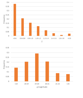
Figure 1: The redshift and g magnitude distribution of the objects.

4 Results

The method described in Section 2 was applied to the data described in Section 3. The method assigns each galaxy that it analyzes with a score of “peculiarity”, and therefore allows to find the galaxies that are the most likely to be indeed peculiar. The 1,100 galaxy images with the highest likelihood to be peculiar according to the method were examined manually, making a selection of $\sim$0.5% of the number of galaxies, but a sufficiently small number of galaxies to allow manual analysis.

Figure 2 shows the top 10 galaxies identified as outlier galaxy images by the algorithm. As can be seen in the image, many of these galaxies are not considered peculiar, but are detected by the algorithm as galaxies that do not have a high number of similar images in the dataset. Due to the presence of a large number of objects that are not outlier galaxies, manual analysis is required for sorting the objects detected by the algorithm. That step of manual analysis removed $\sim$86% of the galaxies that were detected by the algorithm. Figure 3 shows examples of objects that were detected by the algorithm as peculiar, but are not peculiar objects by manual inspection. As the figure shows, these objects include objects that are not rare and can be considered false positives, as well as objects that their peculiarity is not clear of is not of astronomical origin. Because the “peculiarity” of a galaxy is not strictly defined, it is possible that some objects of interest were rejected, but the prevalence of such objects is expected to be low.

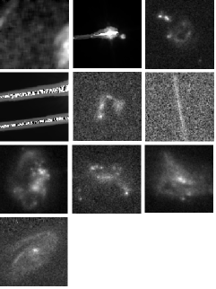
Figure 2: The top 10 outlier galaxy images as ranked by the algorithm.

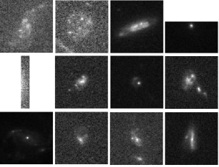
Figure 3: Objects identified by the algorithm as outliers that are not indeed outlier galaxy images.

The algorithm reduces the data by selecting a subset in which the frequency of outlier galaxy images is far higher than in the entire dataset, making the manual analysis practical also for larger datasets. Figure 4 shows the number of objects detected manually among the objects detected automatically, ranked by their distance as described in Section 2. Naturally, the number of detected objects increases when the number of objects being inspected manually gets larger. But the graph also shows that the frequency of detected objects is higher among the galaxies with lower rank, therefore making it practical to perform manual analysis of the results.

Figure 4: The frequency of the number of objects detected manually among the objects detected by the algorithm.

Tables 1 through 9 show the galaxies identified by the algorithm after removing manually $\sim$86% of the objects that are not peculiar galaxies. Figures 5 through 14 show the corresponding images of the objects in the tables. The objects are separated into different types such as gravitational lenses, ring galaxies, objects with embedded point sources, interacting systems, objects with linear features, one-arm galaxies, galaxies with detached segments, tidally distorted interacting galaxies, and other galaxies.

Figure 8 shows edge-on galaxies with dust lanes. These systems are not considered necessarily peculiar, but according to the results these forms are relatively rare in the HST sample. Figure 5 shows detected galaxies with embedded object. Giants clumps of stars embedded in galaxies are not rare in $0.5<z<3$ (Guo et al., 2015). However, while many galaxies can have clumps of stars with no apparent unusual morphology as shown in Figure 6, many of the galaxies in Figure 5 also have an unusual morphology that is different from the morphology of most galaxies with embedded bright clumps of stars. It is therefore possible that the morphology of these galaxies is the reason they are detected, rather than the clumps of stars embedded in them.

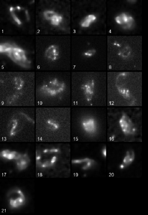
Figure 5: Images of the detected objects listed in Table 1.

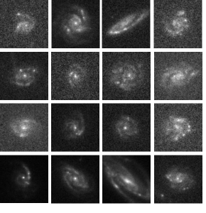
Figure 6: Galaxies with clumps of stars that are not of apparent unusual morphology. These galaxies are very common in the HST sample, and were not detected by the algorithm.

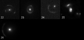
Figure 7: Images of the objects suspected as gravitational lenses listed in Table 2.

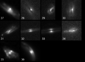
Figure 8: Images of the detected edge-on galaxies with dust lanes listed in Table 3.

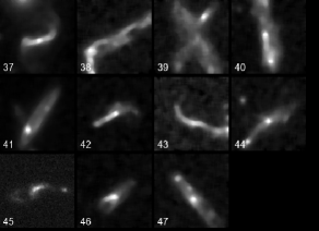
Figure 9: Images of the detected objects with linear features listed in Table 4.

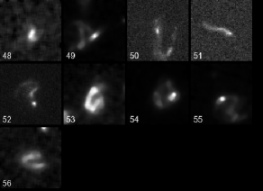
Figure 10: Images of the detected objects listed in Table 5.

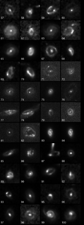
Figure 11: Images of detected galaxies with ring features listed in Table 6.

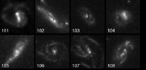
Figure 12: Images of the detected spiral galaxies with detached segments listed in Table 7.

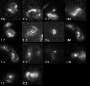
Figure 13: Images of the tidally distorted object candidates listed in Table 8.

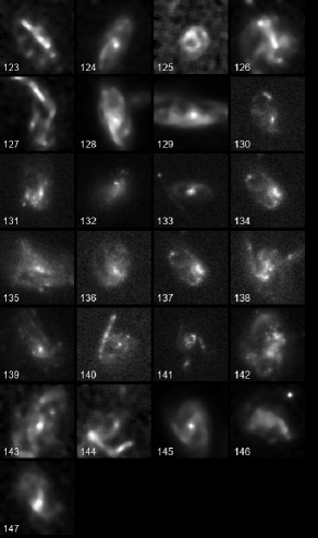
Figure 14: Images of the other detected objects listed in Table 9.

HST can provide details that cannot be obtained by Earth-based sky surveys, and therefore in many cases galaxies that seem visually peculiar in HST do not seem unusual when observed using Earth-based instruments. Figure 15 shows several object in HST, SDSS and Pan-STARRS. As the comparison shows, SDSS and Pan-STARRS do not give sufficient details to identify the morphological features of these galaxies.

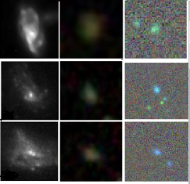
Figure 15: Comparison of objects 128, 139 and 135 images in HST (left), SDSS (middle), and Pan-STARRS (right). As expected, the comparison shows that the Earth-based sky surveys do not provide sufficient details to identify the morphology of these galaxies.

Table 2 shows objects suspected as gravitational lenses. None of these suspected gravitational lenses are included in the CASTLES survey of gravitational lenses (Kochanek et al., 1999), the catalogue of gravitational lens candidates in SDSS (Inada et al., 2012), or a survey powered by a group finding algorithm (Wilson et al., 2016). Two of the objects, 23 and 24, are included in the gravitational lens catalogue of (Faure et al., 2008).

ID	RA	Dec		ID	RA	Dec		ID	RA	Dec
1	189.1622	62.1883		2	215.1411	52.9442		3	189.1906	62.2452
4	188.9980	62.1668		5	53.15489	-27.857		6	150.3146	1.68395
7	150.1713	1.62978		8	150.2772	1.91924		9	150.0289	1.88902
10	149.9010	1.85073		11	150.0291	2.03546		12	149.9216	2.20603
13	150.0966	2.50137		14	150.0506	2.47750		15	150.7432	2.66317
16	53.05503	-27.699		17	189.0773	62.2508		18	53.06687	-27.883
19	189.1166	62.2854		20	53.07838	-27.878		21	189.1230	62.1130

Table 1: The coordinates of detected objects with embedded point sources.

ID	RA	Dec		ID	RA	Dec		ID	RA	Dec
22	149.8789	2.57436		23	150.1594	2.69273		24	150.0772	2.64584
25	53.00104	-27.770		26	34.40478	-5.2248

Table 2: Right ascension and declination (in degrees) of the galaxies suspected as gravitational lenses detected in the dataset.

ID	RA	Dec		ID	RA	Dec		ID	RA	Dec
27	215.3761	53.1241		28	149.8313	1.59189		29	150.0589	1.74697
30	150.0610	1.64515		31	150.3063	1.81053		32	149.8813	1.88521
33	149.8668	2.05173		34	150.2041	2.80623		35	189.0973	62.2924
36	53.07250	-27.822

Table 3: Celestial coordinates of objects that are possible edge-on galaxies with dust lanes.

ID	RA	Dec		ID	RA	Dec		ID	RA	Dec
37	215.2375	53.0477		38	215.2534	53.0987		39	215.1405	53.0041
40	189.1852	62.1949		41	189.2101	62.3432		42	53.12404	-27.878
43	189.2438	62.1366		44	189.2722	62.1792		45	150.6507	1.64533
46	189.0420	62.2196		47	188.9525	62.1982

Table 4: Coordinates of detected objects with linear features.

ID	RA	Dec		ID	RA	Dec		ID	RA	Dec
48	214.8828	52.8360		49	189.2587	62.3045		50	150.6613	1.64342
51	150.2551	1.88673		52	150.1958	1.88558		53	189.3390	62.1921
54	189.0522	62.2440		55	189.1127	62.2995		56	34.31388	-5.2024

Table 5: Coordinates of objects that are possible one-arm galaxies.

ID	RA	Dec		ID	RA	Dec		ID	RA	Dec
57	214.9668	52.8542		58	189.1523	62.2768		59	214.6585	52.7311
60	214.6977	52.6933		61	214.6236	52.7394		62	214.6959	52.7275
63	215.0946	52.9053		64	214.9997	52.9886		65	215.0564	53.0715
66	215.3878	53.1364		67	215.1373	53.0894		68	53.12042	-27.757
69	189.2676	62.2110		70	189.2785	62.1685		71	150.1785	1.62206
72	150.4450	1.72180		73	150.3991	1.62907		74	150.1361	1.67666
75	149.7003	1.67250		76	150.1600	1.92169		77	150.1017	2.05326
78	149.9335	2.04432		79	149.8189	2.07964		80	150.6226	2.24475
81	149.6272	2.19739		82	150.4789	2.40455		83	150.2822	2.46019
84	150.2822	2.46019		85	149.8462	2.85215		86	149.7706	2.80442
87	189.3322	62.1755		88	53.19657	-27.863		89	189.3906	62.2292
90	53.22027	-27.854		91	53.05081	-27.679		92	189.1096	62.1963
93	189.1269	62.2739		94	189.1349	62.1262		95	189.1359	62.1229
96	53.01292	-27.718		97	34.32599	-5.2154		98	34.39667	-5.2660
99	34.26670	-5.1327		100	34.32900	-5.1332

Table 6: Galaxies with ring features.

ID	RA	Dec		ID	RA	Dec		ID	RA	Dec
101	215.2793	53.1822		102	149.9231	1.72376		103	149.7927	1.62935
104	149.6892	1.64355		105	150.6343	1.81815		106	150.4635	1.88330
107	150.4138	1.84758		108	150.5652	2.16613

Table 7: Spiral galaxies with detached segments.

ID	RA	Dec		ID	RA	Dec		ID	RA	Dec
109	53.10084	-27.831		110	215.2063	53.1576		111	53.02481	-27.751
112	189.0039	62.2173		113	189.2672	62.3234		114	150.3090	1.91672
115	150.6876	1.97088		116	149.8947	2.20815		117	149.8947	2.20815
118	150.6845	2.54897		119	149.9031	2.82170		120	189.0672	62.2663
121	189.1247	62.2343		122	34.44746	-5.2467

Table 8: Tidally distorted interacting pairs.

ID	RA	Dec		ID	RA	Dec		ID	RA	Dec
123	215.0012	52.9636		124	189.1776	62.3058		125	215.0720	52.9071
126	214.9257	52.9287		127	215.2056	52.9864		128	215.2513	53.1415
129	53.11494	-27.767		130	150.7439	1.61616		131	150.1504	1.59564
132	149.8757	1.61034		133	150.7142	1.75447		134	149.8485	1.79248
135	149.7127	1.77889		136	149.9777	1.83432		137	149.8485	1.79248
138	150.4372	1.99945		139	150.5846	2.19190		140	149.7653	2.26561
141	150.3849	2.40657		142	150.2759	2.45195		143	189.4095	62.2583
144	189.4532	62.2233		145	189.0520	62.1946		146	34.36355	-5.2133
147	34.31276	-5.1375

Table 9: Other galaxies.

4.1 Differences between regular and outlier galaxy images

Because the analysis is based on numerical image content descriptors, it allows to identify descriptors that can discriminate between regular galaxy images and the outlier images. To identify these descriptors, the image content descriptors of the 147 outlier images were compared to the descriptors of 745 random regular images. The comparison was dine using the Linear Discriminant Analysis (LDA) scores, which can identify the features that can discriminate between the two classes. Table 10 shows some of the numerical image content descriptors with the highest LDA scores, and the means and standard deviation of the regular and outlier galaxy images. The description of the specific descriptors is provided in (Shamir et al., 2008, 2010; Shamir et al., 2013; Schutter & Shamir, 2015; Shamir, 2016).

Descriptor	Regular	Outlier
	mean	mean
Edge area	2796$\pm$171	14578$\pm$ 65
Tamura coarseness	9.59$\pm$0.08	2.43$\pm$0.11
Fractal bin 15	4004$\pm$98	16.79$\pm$0.45
Fractal bin 14	3895$\pm$96	16.13$\pm$0.43
Fractal bin 11	3445$\pm$89	13.32$\pm$0.33
Fractal bin 13	3783$\pm$94	15.46$\pm$0.41
Fractal bin 18	4288$\pm$105	18.57$\pm$0.53
Fractal bin 12	3569$\pm$91	14.06$\pm$0.36

Table 10: The image content descriptors with the highest LDA separation between regular and outlier images.

As the table shows, descriptors such as edge area and Tamura texture coarseness exhibit significant differences between regular and outlier galaxy images. An interesting observation is the fractality, computed by using box counting as described in (Lynch et al., 1991; Shamir et al., 2009). The fractality is much lower among outlier galaxy images compared to the regular images. That indicates that regular galaxies have higher fractality, which drops in the case of outlier images.

4.2 Impact of the value of R

As discussed in Section 2, the value of R is used to avoid the impact of rare objects that have similar objects in the dataset. When analyzing large datasets, even a rare object is expected to appear more than once in the dataset. Therefore, if two rare objects that are very different from all other objects are present in the dataset, it could be that each one of them will be a similar neighbor to the other object. When using the distance from the closest neighbor, the similarity between the two objects will assign each of the objects with a relatively short distance, and therefore these objects might not be detected as peculiar.

To show the impact of the value of R, a simple experiment was done such that the 44 galaxies shown in Figure 11 were combined with galaxies 40 through 44 shown in Figure 9. In that dataset, the ring galaxies are the regular images. When running the algorithm when R is set to 1 and observing the top 10 outliers returned by the algorithm, only objects 40 and 43 are detected among the top five outliers. That does not change when setting the value of R to 2 or 3. But when the value of R is set to 4, all objects 40 through 44 are detected among the top 10 outliers.

4.3 Sensitivity to redshift

The ability of an algorithm to detect outlier galaxy is clearly a function of the redshift. Closer objects are generally brighter and can be observed with better details compared to distant object. It is expected that many objects with rare morphology at high redshift would not be identified as outliers by an algorithm or even by manual observation due to the small size and faint magnitude. Figure 16 shows the number of objects selected by the algorithm in each redshift range divided by the total number of objects detected by the algorithm. If also shows the number of objects determined as outlier candidates after manual inspection in each redshift range, divided by the total number of outlier candidates.

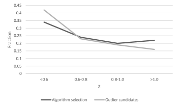
Figure 16: The fraction of objects detected by the algorithm in different redshift ranges compared to the total number of objects detected by the algorithm, and the fraction of outlier candidates in each redshift range compared to the total number of outlier candidates determined after manual inspection. In the lower redshifts the fraction of outlier candidates is higher, while it is getting lower in the higher redshifts.

As the figure shows, the fraction of the objects selected after manual inspection is higher in the lower redshift ranges compared to the general population of objects selected by the algorithm, and lower in the higher redshift ranges of $z>1$. That distribution shows that a higher number of objects in the higher redshifts are detected by the algorithm but rejected after manual inspection, which indicates that in the higher redshifts the algorithm is less effective in identifying outlier galaxy candidates compared to the lower redshifts. That pattern can be expected given that galaxies at higher redshifts tend to be more difficult to inspect visually.

5 Conclusions

Sky surveys can acquire substantial amounts of information that includes a very large number of galaxies. While it can be assumed that these databases contain rare objects of scientific interest, it is difficult to identify these objects among a large number of objects. Here an automatic method is applied to HST data, and identified several unusual extra-galactic objects. While the last step is manual, the algorithm reduces the data by two orders of magnitude, making the manual analysis practical. The objects identified by the algorithm can be used as target in future studies.

The catalogue is clearly incomplete, as the algorithm is not able to identify all rare objects of interest. For instance, just two gravitational lenses detected from the 67 detected gravitational lenses included in the catalogue of (Faure et al., 2008). However, since it is based on automation, it does not require substantial labor, and can therefore be applied in cases where the databases are far too large to allow manual analysis.

With the increasing importance of large-field surveys such as the ground-based Vera Rubin Observatory and the space-based Euclid, it is clear that manual analysis will not be sufficient to fully utilize the extreme imaging power of these instruments. While the efficacy of computer analysis cannot yet meet the accuracy level of manual analysis of an expert, computer analysis is required to approach these extremely large databases, and the ability to use the data acquired by current and future sky surveys is largely dependent on the availability and advancement of algorithm that can practically analyze these data.

Data availability

The data underlying this article are available in the article. The research is based on observations made with the NASA/ESA Hubble Space Telescope, and obtained from the Hubble Legacy Archive, which is a collaboration between the Space Telescope Science Institute (STScI/NASA), the Space Telescope European Coordinating Facility (ST-ECF/ESA) and the Canadian Astronomy Data Centre (CADC/NRC/CSA).

References

- Abraham & van den Bergh (2001) Abraham R. G., van den Bergh S., 2001, Science, 293, 1273
- Abraham et al. (2003) Abraham R. G., Van Den Bergh S., Nair P., 2003, Astrophysical Journal, 588, 218
- Amarbayasgalan et al. (2018) Amarbayasgalan T., Jargalsaikhan B., Ryu K. H., 2018, Applied Sciences, 8, 1468
- Arp (1966) Arp H., 1966, Astrophysical Journal Supplement Series, 14, 1
- Arp & Madore (1975) Arp H. C., Madore B. F., 1975, The Observatory, 95, 212
- Banerji et al. (2010) Banerji M., et al., 2010, Monthly Notices of the Royal Astronomical Society, 406, 342
- Berriman et al. (2004) Berriman G., et al., 2004, in Astronomical Data Analysis Software and Systems. p. 593
- Bertin & Arnouts (1996) Bertin E., Arnouts S., 1996, Astronomy and Astrophysics, 117, 393
- Bettoni et al. (2001) Bettoni D., Galletta G., García-Burillo S., Rodríguez-Franco A., 2001, Astronomy & Astrophysics, 374, 421
- Buta (2017) Buta R. J., 2017, Monthly Notices of the Royal Astronomical Society, 471, 4027
- Casasola et al. (2004) Casasola V., Bettoni D., Galletta G., 2004, Astronomy & Astrophysics, 422, 941
- Cecotti (2020) Cecotti H., 2020, International Journal of Machine Learning and Cybernetics, pp 1–15
- Chen et al. (2018) Chen Z., Yeo C. K., Lee B. S., Lau C. T., Jin Y., 2018, Neurocomputing, 309, 192
- Cheng et al. (2020) Cheng T.-Y., et al., 2020, Monthly Notices of the Royal Astronomical Society, 493, 4209
- Conselice (2003) Conselice C. J., 2003, Astrophysical Journal Supplement Series, 147, 1
- Davis & Hayes (2014) Davis D. R., Hayes W. B., 2014, Astrophysical Journal, 790, 87
- Dieleman et al. (2015) Dieleman S., Willett K. W., Dambre J., 2015, Monthly Notices of the Royal Astronomical Society, 450, 1441
- Faure et al. (2008) Faure C., et al., 2008, Astrophysical Journal Supplement Series, 176, 19
- Finkelman et al. (2012) Finkelman I., Funes SJ J. G., Brosch N., 2012, Monthly Notices of the Royal Astronomical Society, 422, 2386
- Fogel & Sagi (1989) Fogel I., Sagi D., 1989, Biological Cybernetics, 61, 103
- Gillman et al. (2020) Gillman S., et al., 2020, Monthly Notices of the Royal Astronomical Society, 492, 1492
- Goddard & Shamir (2020) Goddard H., Shamir L., 2020, Astrophysical Journal Supplement Series, 251, 28
- Graham (2019) Graham A. W., 2019, Monthly Notices of the Royal Astronomical Society, 487, 4995
- Grogin et al. (2011) Grogin N. A., et al., 2011, Astrophysical Journal Supplement Series, 197, 35
- Guo et al. (2015) Guo Y., et al., 2015, Astrophysical Journal, 800, 39
- Hadjidemetriou et al. (2001) Hadjidemetriou E., Grossberg M. D., Nayar S. K., 2001, in Proceedings of the IEEE Computer Society Conference on Computer Vision and Pattern Recognition. pp I–I
- Haralick et al. (1973) Haralick R. M., Shanmugam K., Dinstein I. H., 1973, IEEE Transactions on Systems, Man, and Cybernetics, pp 610–621
- Hosny et al. (2020) Hosny K., Elaziz M., Selim I., Darwish M., 2020, Astronomy and Computing, p. 100383
- Huertas-Company et al. (2009) Huertas-Company M., et al., 2009, Astronomy and Astrophysics, 497, 743
- Huertas-Company et al. (2015a) Huertas-Company M., et al., 2015a, arXiv preprint arXiv:1509.05429
- Huertas-Company et al. (2015b) Huertas-Company M., et al., 2015b, arXiv preprint arXiv:1506.03084
- Inada et al. (2012) Inada N., et al., 2012, Astronomical Journal, 143, 119
- Jacobs et al. (2019) Jacobs C., et al., 2019, Monthly Notices of the Royal Astronomical Society, 484, 5330
- Kaviraj (2010) Kaviraj S., 2010, Monthly Notices of the Royal Astronomical Society, 406, 382
- Kochanek et al. (1999) Kochanek C., Falco E., Impey C., Lehár J., McLeod B., Rix H.-W., 1999, in AIP Conference Proceedings. pp 163–175
- Koekemoer et al. (2011) Koekemoer A. M., et al., 2011, Astrophysical Journal Supplement Series, 197, 36
- Kuminski & Shamir (2016) Kuminski E., Shamir L., 2016, Astrophysical Journal Supplement Series, 223, 20
- Kuminski et al. (2014) Kuminski E., George J., Wallin J., Shamir L., 2014, Publications of the Astronomical Society of the Pacific, 126, 959
- Lim (1990) Lim J. S., 1990, New Haven: Prentice Hall
- Lintott et al. (2009) Lintott C. J., et al., 2009, Monthly Notices of the Royal Astronomical Society, 399, 129
- Lynch et al. (1991) Lynch J., Hawkes D., Buckland-Wright J., 1991, Physics in Medicine & Biology, 36, 709
- Madore et al. (2009) Madore B. F., Nelson E., Petrillo K., 2009, Astrophysical Journal Supplement Series, 181, 572
- Margalef-Bentabol et al. (2020) Margalef-Bentabol B., Huertas-Company M., Charnock T., Margalef-Bentabol C., Bernardi M., Dubois Y., Storey-Fisher K., Zanis L., 2020, arXiv:2003.08263
- Margapuri et al. (2020) Margapuri V. S. K., Shamir L., Thapa B., 2020, in 29th International Conference on Software Engineering and Data Engineering.
- Mittal et al. (2019) Mittal A., Soorya A., Nagrath P., Hemanth D. J., 2019, Earth Science Informatics, pp 1–17
- Nair & Abraham (2010) Nair P. B., Abraham R. G., 2010, Astrophysical Journal Supplement Series, 186, 427
- Nairn & Lahav (1997) Nairn A., Lahav O., 1997, Monthly Notices of the Royal Astronomical Society, 286, 969
- Peng et al. (2002) Peng C. Y., Ho L. C., Impey C. D., Rix H.-W., 2002, Astronomical Journal, 124, 266
- Rubner et al. (2000) Rubner Y., Tomasi C., Guibas L. J., 2000, International Journal of Computer Vision, 40, 99
- Ruzon & Tomasi (2001) Ruzon M. A., Tomasi C., 2001, IEEE Transactions on Pattern Analysis and Machine Intelligence, 23, 1281
- Schutter & Shamir (2015) Schutter A., Shamir L., 2015, Astronomy and Computing, 12, 60
- Scoville et al. (2007) Scoville N., et al., 2007, Astrophysical Journal Supplement Series, 172, 1
- Shamir (2009) Shamir L., 2009, Monthly Notices of the Royal Astronomical Society, 399, 1367
- Shamir (2011) Shamir L., 2011, Astrophysical Journal, 736, 141
- Shamir (2012) Shamir L., 2012, Journal of Computational Science, 3, 181
- Shamir (2016) Shamir L., 2016, Publications of the Astronomical Society of the Pacific, 129, 024003
- Shamir (2017) Shamir L., 2017, Astrophysics Source Code Library, p. ascl:1704.002
- Shamir (2020) Shamir L., 2020, Monthly Notices of the Royal Astronomical Society, 491, 3767
- Shamir & Wallin (2014) Shamir L., Wallin J., 2014, Monthly Notices of the Royal Astronomical Society, 443, 3528
- Shamir et al. (2008) Shamir L., Orlov N., Eckley D. M., Macura T., Johnston J., Goldberg I. G., 2008, Source Code for Biology and Medicine, 3, 13
- Shamir et al. (2009) Shamir L., Ling S. M., Scott W., Hochberg M., Ferrucci L., Goldberg I. G., 2009, Osteoarthritis and Cartilage, 17, 1307
- Shamir et al. (2010) Shamir L., Macura T., Orlov N., Eckley D. M., Goldberg I. G., 2010, ACM Transactions on Applied Perception, 7, 1
- Shamir et al. (2013) Shamir L., Holincheck A., Wallin J., 2013, Astronomy and Computing, 2, 67
- Simard (1999) Simard L., 1999, in Photometric Redshifts and the Detection of High Redshift Galaxies. p. 325
- Tamura et al. (1978) Tamura H., Mori S., Yamawaki T., 1978, IEEE Transactions on Systems, Man, and Cybernetics, 8, 460
- Taylor et al. (2005) Taylor V. A., Jansen R. A., Windhorst R. A., Odewahn S. C., Hibbard J. E., 2005, Astrophysical Journal, 630, 784
- Teague (1980) Teague M. R., 1980, Journal of the Optical Society of America, 70, 920
- Timmis & Shamir (2017) Timmis I., Shamir L., 2017, Astrophysical Journal Supplement Series, 231, 2
- Wilson et al. (2016) Wilson M. L., Zabludoff A. I., Ammons S. M., Momcheva I. G., Williams K. A., Keeton C. R., 2016, Astrophysical Journal, 833, 194
- Wu et al. (1992) Wu C.-M., Chen Y.-C., Hsieh K.-S., 1992, IEEE Transactions on Medical Imaging, 11, 141