Meson and glueball spectroscopy within the graviton soft wall model

Abstract

The graviton soft wall model (GSW) provides a unified description of the scalar glueball and meson spectra with a unique energy scale. This success has led us to extend the analysis to the description of the spectra of other hadrons. We use this model to calculate masses of the odd and even ground states of glueballs for various spins, and show that the GSW model is able to reproduce the Regge trajectory of these systems. In addition, the spectra of the $\rho$, $a_{1}$ and the $\eta$ mesons will be addressed. Results are in excellent agreement with current experimental data. Furthermore such an achievement is obtained without any additional parameters. Indeed, the only two parameters appearing in these spectra are those that were previously fixed by the light scalar meson and glueball spectra. Finally, in order to describe the $\pi$ meson spectrum, a suitable modification of the dilaton profile function has been included in the analysis to properly take into account the Goldstone realization of chiral symmetry. The present investigation confirms that the GSW model provides an excellent description of the spectra of mesons and glueballs with only a small number of parameters unveiling a relevant predicting power.

I Introduction

In the last few years, hadronic models, inspired by the holographic conjecture Maldacena (1999); Witten (1998), have been vastly used and developed in order to investigate non-perturbative features of glueballs and mesons, thus trying to grasp fundamental features of QCD Fritzsch et al. (1973); Fritzsch and Minkowski (1975). Recently we have used the so called AdS/QCD models to study the scalar glueball spectrum Vento (2017); Rinaldi and Vento (2018). The holographic principle relies in a correspondence between a five dimensional classical theory with an AdS metric and a supersymmetric conformal quantum field theory with $N_{C}\rightarrow\infty$. This theory, different from QCD, is taken as a starting point to construct a 5 dimensional holographic dual of it. This is the so called bottom-up approach Polchinski and Strassler (2000); Brodsky and de Téramond (2004); Da Rold and Pomarol (2005); Karch et al. (2006). In this scenario, models are constructed by modifying the five dimensional classical AdS theory with the aim of resembling QCD as much as possible. The main differences characterizing these models are related to the strategy used to break conformal invariance. Moreover, it must be noted that the relation which these models establish with QCD is at the level of the leading order in the number of colours expansion, and thus the mesonic and glueball spectrum and their decay properties are ideal observables to be studied by these models.

Being the mesons and glueball masses $\mathcal{O}(N_{C}^{0})$, the AdS/QCD models reproduce the essential features of the meson and glueball spectrum Erlich et al. (2005); Colangelo et al. (2008); de Teramond and Brodsky (2005); Rinaldi and Vento (2018); Colangelo et al. (2007); Folco Capossoli and Boschi-Filho (2016). For mesons and baryons, these approaches have been also successfully used to describe form factors and various types of parton distribution functions de Teramond and Brodsky (2005); Rinaldi (2017); Bacchetta et al. (2017); de Teramond et al. (2018). Besides these developments, which are in line with the present investigation, other models have been recently introduced by using the bottom-up holography. For example, an interesting development is the no-wall model Afonin and Pusenkov (2013), which has been successful in explaining the heavy meson spectra.

The present investigation has as its starting point the holographic Soft-Wall (SW) model scheme, were a dilaton field is introduced to softly break conformal invariance. This procedure allows to properly reproduce the Regge trajectories of the meson spectra. Within this scheme we have recently introduced the graviton soft-wall model (GSW) Rinaldi and Vento (2018, 2020a, 2020b) which has been able to reproduce, not only the scalar meson spectrum, but also the lattice QCD scalar glueball masses Morningstar and Peardon (1999); Chen et al. (2006); Lucini et al. (2004), that was not described by the traditional SW models. Moreover, a formalism to study the glueball-meson mixing conditions has been developed and some predictions, regarding the observably of pure glueball states, has been provided  Rinaldi and Vento (2020a, b). The success of the model in reproducing the scalar QCD spectra, has motivated us to extend, in the present investigation, the GSW model to describe the $\rho$ vector meson, the $a_{1}$ axial vector meson, the pseudo-scalar meson spectra and to calculate the Regge trajectories of high spin glueballs. To develop a unified approach where the QCD dynamics of glueballs is encoded in the modified metric, a specific dilaton, providing the correct confining mechanism for a given hadron, is constructed. To this aim, a differential equation for the dilaton field has been obtained, which leads to an effective phenomenological potential that produces a good description of several meson spectra.

In the next section, the modification of the SW model, to obtain the GSW one, is discussed. In particular, in Sect. II we summarise the essence of the GSW model  Rinaldi and Vento (2018, 2020a, 2020b). In Sect. III the GSW model has been applied to estimate the scalar glueball and spin dependent glueball spectra. In the last case the Regge trajectories have been obtained and they compare successfully with lattice data. In Sects. IV-V the scalar spectrum is investigated. To this aim, a procedure to establish a dilaton which provides the correct confining mechanism has been developed. In Sect. VI the $\rho$ spectrum is described and in Sect. VII that of the $a_{1}$ meson will be shown together with a comparison with data. In Sect. VIII the pseudo-scalar meson spectra will be analysed and the GSW results presented. In Sect. IX we discuss and summarise the results of our analysis. Finally, we have included 3 Appendices where the determination of the dilaton equation is described in detail.

II The GSW model

Let us review in this section the essence of the GSW model. The development of this approach has been motivated by the impossibility of the conventional SW models to describe the glueball and meson spectra with the same energy scale Rinaldi and Vento (2018, 2020a, 2020b). The essential feature, which distinguishes the GSW model from the traditional SW, is a deformation of the $AdS$ metric in 5 dimensions.

$$ds^{2}=\frac{R^{2}}{z^{2}}e^{\alpha\phi_{0}(z)}(dz^{2}+\eta_{\mu\nu}dx^{\mu}dx^{\nu})=e^{2A(z)}(dz^{2}+\eta_{\mu\nu}dx^{\mu}dx^{\nu})=e^{\alpha{\phi_{0}(z)}}g_{MN}dx^{M}dx^{N}=\bar{g}_{MN}dx^{M}dx^{N}.$$ (1)

where $A(z)=\log{{R}/{z}}+{\alpha\phi_{0}(z)}/{2}$.

The quantities evaluated in the GSW model will be displayed with overline. The function $\phi_{0}(z)$ will be specified later. This kind of modification has been adopted in many studies of the properties of mesons and glueballs within AdS/QCD  Colangelo et al. (2007); Folco Capossoli and Boschi-Filho (2016); Vega and Cabrera (2016); Akutagawa et al. (2020); Gutsche et al. (2019); Klebanov and Maldacena (2004); Martin Contreras and Vega (2020); Folco Capossoli et al. (2020); Bernardini et al. (2017); Li and Huang (2013). The relation between the standard $AdS_{5}$ metric and $\bar{g}_{MN}$ is

$$\bar{g}^{MN} = e^{-\alpha\phi_{0}(z)}g^{MN},$$ (2)

$$\sqrt{-\bar{g}} = e^{\frac{5}{2}\alpha\phi_{0}(z)}\sqrt{-g}.$$ (3)

Once the gravitational background has been defined by the model, the same strategy used in the SW case is considered to obtain the equations of motion for the different fields dual to given hadronic states. The action, in terms of the standard AdS metric of the SW model, is given by

$$\bar{S}={\int d^{4}xdz~{}e^{-\phi_{0}(z)\beta}\sqrt{-\bar{g}}\mathcal{L}(x_{\mu},z)}=\int d^{4}xdz~{}e^{\phi_{0}(z)\left(\frac{5}{2}\alpha-\beta+1\right)}\sqrt{-g}e^{-\phi_{0}(z)}\mathcal{L}(x_{\mu},z)~{},$$ (4)

where here the prefactor $exp\left[{\phi_{0}(z)\left(\frac{5}{2}\alpha+\beta+1\right)}\right]$ is due to the modification of the metric. The parameters $\alpha$ and $\beta$ parametrise the internal dynamics of the hadrons of QCD in AdS, its holographic dual. In the AdS dynamics, $\alpha$ characterises the modification of the metric, while $\beta$ characterises the SW model dilaton, namely the breaking of conformal invariance. If one considers, as a starting point, the GSW model as a modification of the SW model, one is forced to fix $\beta$ to have the same kinematics Rinaldi and Vento (2018, 2020a, 2020b) which leads, in the case of scalar fields, to $\beta=\beta_{s}=1+\frac{3}{2}\alpha$ and in the case of the vector fields to $\beta=\beta_{\rho}=1+\frac{1}{2}\alpha$. The function $\mathcal{L}(x_{\mu},z)$ is the Lagrangian density representing the hadronic system. In Refs. Erlich et al. (2005); Colangelo et al. (2008); de Teramond and Brodsky (2005); Rinaldi and Vento (2018); Colangelo et al. (2007); Folco Capossoli and Boschi-Filho (2016), the chosen dilaton profile function has been $\phi_{0}(z)=k^{2}z^{2}$ . We start with the same dilaton, however in order to include the chiral symmetry behaviour of the pion, this functional form of the dilaton has to be modified. Details will be discussed in Sect. VI. Moreover, as it will become clear in the next section, in order to properly describe confinement and thus the spectra, a further free parameter addition to the dilaton has been introduced.

We proceed in the next section to describe the spectra of glueballs, and their relative Regge trajectories, and we compare the results of our calculations with lattice data.

III GLUEBALLS IN THE GSW MODEL

This section is dedicated to the successful application of the GSW model to the study of the glueball spectra and its comparison with lattice data.

III.1 Scalar glueballs as gravitons

A peculiarity of the GSW model, which is the reason for the name, is that the scalar glueball arises from the scalar component of the graviton and is not introduced as an independent field. Thus in our scheme the metric characterises the scalar graviton. Therefore the Einstein equation for the metric Eq. (1) is the glueball mode equation. In the 5th-variable $z$ once the $x$ dependence has been factorised as $\Phi(z)e^{ix_{\mu}q^{\mu}}$, where $q^{2}=-M^{2}$ and $M$ represents the mass of the glueball modes becomes,

$$\frac{d^{2}\Phi(z)}{dz^{2}}-\left(\alpha k^{2}z+\frac{3}{z}\right)\frac{d\Phi(z)}{dz}+\left(\frac{8}{z^{2}}-6\alpha k^{2}-4\alpha^{2}k^{4}z^{2}+M^{2}\right)\Phi(z)-\frac{8}{z^{2}}e^{\alpha k^{2}z^{2}}\Phi(z)=0~{}.$$ (5)

By performing the change of function

$$\Phi(z)=e^{\alpha k^{2}z^{2}/4}\left(\frac{z}{\alpha k}\right)^{\frac{3}{2}}\phi(z)$$ (6)

we get a Schrödinger type equation

$$-\frac{d^{2}\phi(z)}{dz^{2}}+\left(\frac{8}{z^{2}}e^{\alpha k^{2}z^{2}}-\frac{15}{4}\alpha^{2}k^{4}z^{2}+7\alpha k^{2}-\frac{17}{4z^{2}}\right)\phi(z)=M^{2}\phi(z).$$ (7)

In this equation it is apparent that $M^{2}$ represents the mode mass squared which will arise from the eigenvalues of a Hamiltonian operator scheme. It is convenient to move to the adimensional variable $t=\sqrt{\alpha k^{2}/2}\;z$ and to define the mode by $\Lambda^{2}=(2/\alpha k^{2})\;M^{2}$. The the equation becomes

$$-\frac{d^{2}\phi(t)}{dt^{2}}+\left(\frac{8}{t^{2}}e^{2t^{2}}-15t^{2}+14-\frac{17}{4t^{2}}\right)\phi(t)=\Lambda^{2}\phi(t).$$ (8)

This is a typical Schrödinger equation with no free parameters except for an energy scale in the mass determined by $\alpha k^{2}$. The potential term is uniquely determined by the metric and only the scale factor is unknown and will be determined from lattice QCD. This equation has no exact solutions but numerical ones have been found Rinaldi and Vento (2018). The above expression can be approximated by expanding the exponential up to second term to get a Kummer type equation. However, such a procedure does not lead to good results and the spectrum turns out to be too flat, see details on Refs. Rinaldi and Vento (2020b). As one can see in the left panel of Fig. 3, for the value $\alpha k^{2}\sim(0.37$ GeV)² the scalar linear glueball spectrum is well reproduced, see also Tab. 4. Let us mention the recent study SDTK Sarantsev et al. (2021); Klempt (2021) where the mass of the ground state of the scalar glueball has been extracted from a phenomenological analysis of the BESIII data of the $J/\Psi$ decays. The result obtained is very close to that predicted by the GSW model Rinaldi and Vento (2020a).

$J^{PC}$	$0^{++}$	$2^{++}$	$0^{++}$	$2^{++}$	$0^{++}$	$0^{++}$
MP	$1730\pm 94$	$2400\pm 122$	$2670\pm 222$
YC	$1719\pm 94$	$2390\pm 124$
LTW	$1475\pm 72$	$2150\pm 104$	$2755\pm 124$	$2880\pm 164$	$3370\pm 180$	$3990\pm 277$
SDTK	$1865\pm 25^{+10}_{-30}$
GSW	$1920$	$2371$	$2830$	$2830$	$3289$	$3740$

Table 1: Scalar glueball masses [MeV] from lattice calculations by MP  Morningstar and Peardon (1999), YC Chen et al. (2006) and LTW  Lucini et al. (2004) and the recent analysis SDTK Sarantsev et al. (2021); Klempt (2021) together with the result of our calculation for $\sqrt{\alpha}k=370$ MeV, obtained by the GSW model Rinaldi and Vento (2020a).

III.2 High Spin Glueballs

In order to describe even and odd high spin glueballs we follow the approach described in Refs. Folco Capossoli and Boschi-Filho (2016); Boschi-Filho et al. (2006); Folco Capossoli et al. (2020). In this case the action, written in terms of pure $AdS_{5}$ five, is the same as that of the scalar case Rinaldi and Vento (2020b):

$$\bar{S}=\int d^{5}x~{}\sqrt{-g}e^{-k^{2}z^{2}}\Big{[}g^{MN}\partial_{M}G(x)\partial_{N}G(x)+e^{\alpha k^{2}z^{2}}M_{5}^{2}R^{2}G(x)\Big{]}~{},$$ (9)

and therefore the equation of motion is obtained from:

$$\partial_{M}(\sqrt{-g}e^{-\phi_{0}(z)}g^{MN}\partial_{N}G(x))=\sqrt{-g}e^{-\phi_{0}(z)(1-\alpha)}M^{2}_{5}R^{2}G(x).$$ (10)

In order to describe a spin $J$ glueballs, one can add $J$ covariant derivatives in the gravity dual operator  de Teramond and Brodsky (2005); Folco Capossoli and Boschi-Filho (2016); Boschi-Filho et al. (2006); Folco Capossoli et al. (2020). Therefore, for an even spin glueball, the operator has the form,

$$\mathcal{O}_{4+j}=FD_{\{\mu 1....}D_{\mu J\}}F,$$ (11)

which is a $p=0$ form whose conformal dimension is $\Delta=4+J$. For the odd spin case, one considers the symmetrized operator,

$$\mathcal{O}_{6+j}=SymTr\Big{(}\tilde{F}_{\mu\nu}FD_{\{\mu 1....}D_{\mu J\}}F\Big{)}~{},$$ (12)

which is also a $p=0$ form whose conformal dimension $\Delta=6+J$. By using, the relation between the conformal dimension and the mass in five dimensions Eq.(24), since the glueballs are p-forms of index $p=0$, one gets that for even spin glueballs,

$$M_{5}^{2}R^{2} =J(J+4)\;\mbox{for even}~{}J~{};$$ (13)

and for the odd spin glueballs

$$M_{5}^{2}R^{2} =(J+2)(J+6)\;\mbox{for odd}~{}J.$$ (14)

In this framework, the EoM for the glueballs can be rearranged in a Schrödinger type equation:

$$-\psi^{\prime\prime}(z)+\left[\dfrac{B^{\prime}(z)^{2}}{4}-\dfrac{B^{\prime\prime}(z)}{2}+\dfrac{M_{5}^{2}R^{2}}{z^{2}}e^{\alpha k^{2}z^{2}}\right]\psi(z)=M^{2}\psi(z)~{}.$$ (15)

where, $A(z)=\log(R/z)+{\alpha\phi_{0}}/{2}$ and $B(z)=-\phi(z)-3A(z)$, being again $\phi(z)=\beta_{s}k^{2}z^{2}$. The above equation leads to

$$-\psi^{\prime\prime}(z)+\left[\left(\beta_{s}+\frac{3\alpha}{2}\right)^{2}k^{4}z^{2}-2\left(\beta_{s}+\frac{3\alpha}{2}\right)k^{2}+\dfrac{15}{4z^{2}}+\dfrac{M_{5}^{2}R^{2}}{z^{2}}e^{\alpha k^{2}z^{2}}\right]\psi(z)=M^{2}\psi(z)~{}.$$ (16)

In this case, since $M_{5}^{2}R^{2}\geq 0$, see Eqs. (13, 14), the exponential term is positive and therefore the potential is binding. The exact equation can be numerically solved for bound states. Results of the calculations for the odd and even glueballs are shown in Table 2 and 3, respectively, and will be discussed later. Let us recall that in our formalism for the scalars $\beta_{s}=1+\frac{3}{2}\alpha$.

III.3 Odd glueballs

Despite the lack of the data related to glueballs with $J\geq 1$ spin, several QCD lattice and model calculation are at our disposal  Morningstar and Peardon (1999); Chen et al. (2006); Meyer (2004); Gregory et al. (2012); Llanes-Estrada et al. (2006); Mathieu et al. (2008a); Szanyi et al. (2020); Szczepaniak and Swanson (2003); Mathieu et al. (2008b); Landshoff (2001); Meyer and Teper (2005). In order to evaluate this spectrum within the GSW model, Eq. (16) should be solved to find the lowest mode corresponding to $n=0$ and for $M_{5}^{2}R^{2}=(J+2)(J+6)$. In Table 2 we compare the results of our calculations for the ground states with a series of lattice results and model calculations and we see that we obtain a quite good agreement with them. Also in this case let us remark that this is a parameter free calculation. Indeed, $\alpha$ and $k$, the only parameters of the model, have been fixed by the spectra of the scalar glueballs and light scalar mesons Rinaldi and Vento (2020b). The latter remark will be discussed in the next section. It is important to stress that the present calculation is not a fit to the data but a direct evaluation of the spectrum without any free parameters. From our results, shown in Tab. 2, one can derive the Regge trajectories:

$$J\sim 0.18\pm 0.01M^{2}-0.75\pm 0.28\;$$ (17)

where $M$ here is in GeV, result to be compared with that of Ref. Llanes-Estrada et al. (2006),

$$J\sim 0.18M^{2}+0.25~{}.$$ (18)

$J^{PC}$	M&P	Ky	My	Ll	Mta	Sz	This work	Ref. Bernardini et al. (2017)	Ref. Folco Capossoli et al. (2020)
$1^{--}$	$3850\pm 140$	$3830\pm 130$	$3240\pm 480$	$3950$	$3990$	3001	$3308\pm 15$	2400	2630
$3^{--}$	$4130\pm 290$	$4200\pm 245$	$4330\pm 460$	$4150$	$4160$	$4416$	$4451\pm 12$	3030	3700
$5^{--}$				$5050$	$5260$	$5498$	$5752\pm 10$	5010	4740
$7^{--}$				$5900$			$6972\pm\;8$	7000	5780

Table 2: Comparison of the masses of the ground states for the odd spin glueballs (in MeV) from the following sources, M&P Morningstar and Peardon (1999), Ky Chen et al. (2006), My Meyer (2004), Ll Llanes-Estrada et al. (2006), Mta Mathieu et al. (2008a), Sz Szanyi et al. (2020), with the results of the GSW model We also show results obtained by the models of Refs. Folco Capossoli et al. (2020); Bernardini et al. (2017).

III.4 Even glueballs

We calculate here the spectrum for even spin glueballs by means of Eqs. (16) and (13) In this case, $M_{5}^{2}R^{2}=J(J+4)$. Let us remind that for this sector lattice data of both the ground and excited states for the $0^{++}$ and $2^{++}$ are available together with that of the ground states of $4^{++}$ and $6^{++}$ states. The interpretation of the spectrum of the $0^{++}$ was the motivation behind the formulation of the GSW model  Rinaldi and Vento (2018, 2020a, 2020b) and has been thoroughly studied, thus here we discuss the behaviour of the ground state of the $2^{++},4^{++},6^{++}$ glueballs. As one can see in Tab. 3, the ground states are well reproduced. From the results shown in Tab. 3, one can derive the Regge trajectories,

$J^{PC}$	M&P	Ky	My	Gy	Sk	Mtb	This work	Ref. Folco Capossoli et al. (2020)
$2^{++}$	$2400\pm 145$	$2390\pm 150$	$2150\pm 130$	$2620\pm 50$	$2420$	$2590$	$2695\pm 21$	2080
$4^{++}$			$3640\pm 150$		$3990$	$3770$	$3920\pm 14$	3170
$6^{++}$			$4360\pm 460$			$4600$	$5141\pm 12$	4220

Table 3: Comparison of the masses of the ground states for the even spin glueballs (in MeV) from the following sources, M&P Morningstar and Peardon (1999), Ky Chen et al. (2006), My Meyer (2004), GyGregory et al. (2012), Sk Szczepaniak and Swanson (2003), Mtb Mathieu et al. (2008b), with the results of the GSW model and that of the approach of Ref. Folco Capossoli et al. (2020).

$$J\sim(0.21\pm 0.01)M^{2}+0.58\pm 0.34,$$ (19)

where $M$ is here in GeV. The slope is in reasonable agreement with Refs. Landshoff (2001); Meyer and Teper (2005), i.e., $0.25$.

In Table 4 we show the lattice data the graviton solution (GSW) , the J = 0 solution GSW0 and the J = 2 solution for the same values of the parameters as before (GSW2). The graviton solution describes the data well, while the J = 0 and the J=2 solutions do not. One cannot try to justify the discrepancy in terms of the chosen energy scale since the J=0 solution would require a higher energy scale while the J=2 solution a lower. Somehow the graviton with its degeneracy between scalar and tensor seems to contain the appropriate physics.

$J^{PC}$	$0^{++}$	$2^{++}$	$0^{++}$	$2^{++}$	$0^{++}$	$0^{++}$
MP	$1730\pm 94$	$2400\pm 122$	$2670\pm 222$
YC	$1719\pm 94$	$2390\pm 124$
LTW	$1475\pm 72$	$2150\pm 104$	$2755\pm 124$	$2880\pm 164$	$3370\pm 180$	$3990\pm 277$
SDTK	$1865\pm 25^{+10}_{-30}$
GSW	$1920$	$2371$	$2830$	$2830$	$3289$	$3740$
GSW0	$1411\pm 52$		$1728\pm 67$		$1995\pm 79$	$2231\pm 86$
GSW2		$2695\pm 21$		$3179\pm 20$

Table 4: Glueball masses [MeV] from lattice calculations by MP  Morningstar and Peardon (1999), YC Chen et al. (2006), LTW  Lucini et al. (2004) and the recent analysis SDTK Sarantsev et al. (2021); Klempt (2021) compared with the graviton (GSW) and field (GSW0 and GSW2) correspondences .

IV THE SCALAR MESON SPECTRUM

In this section we present the results of the calculations of the light and heavy scalar meson spectra within the GSW model. In the light sector we get the following Equation of Motion (EoM) Rinaldi and Vento (2020b)),

$$\partial_{M}(\sqrt{-g}e^{-\phi_{0}(z)}g^{MN}\partial_{N}S(x,z))=\sqrt{-g}e^{-\phi_{0}(z)(1-\alpha)}M^{2}_{5}R^{2}S(x,z).$$ (20)

Once we separate the $x$ dependence by factorising $S(x,z)=\Sigma(z)e^{-iq_{\mu}x^{\mu}}$ with $q^{2}=-M^{2}$, where $M$ is the mass of the meson modes, we get

$$-\frac{d^{2}\Sigma(z)}{dz^{2}}+\left(\frac{3}{z}+2k^{2}z\right)\frac{d\Sigma(z)}{dz}-\frac{M_{5}^{2}R^{2}}{z^{2}}e^{\alpha\phi_{0}(z)}\Sigma(z)=M^{2}\Sigma(z)~{}.$$ (21)

By recalling that $\phi_{0}(z)=k^{2}z^{2}$ and performing the change of function

$$\Sigma(z)=\left(\frac{z}{k}\right)^{\frac{3}{2}}e^{k^{2}z^{2}/2}\sigma(z),$$ (22)

a Schrödinger type equation can be obtained,

$$-\frac{d^{2}\sigma(z)}{dz^{2}}+V_{s}(z)\sigma(z)=-\frac{d^{2}\sigma(z)}{dz^{2}}+\left(k^{4}z^{2}+2k^{2}+\frac{15}{4z^{2}}-\frac{3}{z^{2}}e^{\alpha k^{2}z^{2}}\right)\sigma(z)=M^{2}\sigma(z).$$ (23)

For the scalar meson, the AdS mass is

$$M_{5}^{2}R^{2}=(\Delta-p)(\Delta+p-4)$$ (24)

where $\Delta$ is the conformal dimension and $p$ the p-form index. For the scalar field $M_{5}^{2}R^{2}=-3$ since the $\Delta=3$ and $p=0$ Martin Contreras et al. (2020).

The potential of the above equation, obtained with the same procedure used for the glueballs, is in this case not binding, as shown by the full line of Fig. 1. Indeed, since for scalar mesons the conformal mass is negative, the exponential term in Eq. (23) prevents the system to bind. However, in Ref. Rinaldi and Vento (2020b), it has been shown that if the above potential is Taylor expanded for small values of $\alpha$, up to the first three terms, a binding potential related to the glueball dynamics of QCD described by the metric Eq. (1), can be obtained. In the next section a formal procedure to motivate such a truncation will be presented together with its physical interpretation.

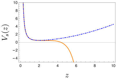
Figure 1: The full potential in Eq. (23) is shown by the solid line and the dot-dashed line shows the potential arising from the series expansion of the potential around small values of $\alpha$ keeping the first three terms. The figures shown have been obtained for $\alpha=0.55$.

V New dilaton and a phenomenological potential for mesons

In this section we present a new procedure to coherently describe the glueball and the meson spectra within the GSW model, i.e. the same metric. In fact, as previously discussed, at the variance with the spin dependent glueball, where the conformal mass is positive and thus the metric (1) leads to a confining potential, in the meson sector, the relative potential is not binding due to negative the conformal mass. However, it has been shown that if this potential is truncated after a Taylor expansion for small values of $\alpha$, the potential confines and the spectrum is very well reproduced Rinaldi and Vento (2020b). Therefore, in this section we show how the approximated potential can be obtained. Let us remark that the latter quantity is very appealing because, as discussed in Ref. Rinaldi and Vento (2020b), it leads to a very good description of the light and heavy meson spectra with only one free parameter, $\alpha$, since the scale parameter $\alpha k^{2}$ was fixed by the spectrum of the scalar glueball Rinaldi and Vento (2018). In this framework, we point out that the procedure here introduced will not make use of any additional free parameter and the only restriction consists in obtaining the convenient effective potential for the scalar meson EoM. Let us anticipate that, as it will be shown in the next sections, this type of potential allows to reproduce the spectra of various meson families without introducing any ad-hoc parameters. To this aim, we consider a modification of the dilaton in the meson sector. In the following we consider the scalar case, however, as shown in Appendices A-C, the results can be generalised to the vector sector and to the pion, which will require a specific prescription to describe chiral-symmetry breaking.

Let us consider an extension of Eq. 4 for the scalar meson,

$$\bar{S}=\int d^{5}x~{}\sqrt{-g}e^{-\phi_{0}(z)-\phi_{n}(z)}\Big{[}g^{MN}\partial_{M}S(x)\partial_{N}S(x)+e^{\alpha\phi_{0}(z)}M_{5}^{2}R^{2}S^{2}(x)\Big{]}~{},$$ (25)

where we recall that $\phi_{0}=\ k^{2}z^{2}$. Furthermore, we denote by $\phi_{n}$ an addition to the dilaton $\phi_{0}$ with the purpose of generating the effective potential. The relative EoM is now,

$$\partial_{M}\Big{[}\sqrt{-g}e^{-\phi_{0}(z)-\phi_{n}(z)}g^{MN}\partial_{N}S(x)\Big{]}-\sqrt{-g}M_{5}^{2}R^{2}e^{\alpha\phi_{0}(z)-\phi_{n}(z)}S(x)=0~{}.$$ (26)

Then potential in the corresponding Schrödinger equation reads,

$$V_{s}(z)=\frac{15}{4z^{2}}+M_{5}^{2}R^{2}\frac{e^{\alpha k^{2}z^{2}}}{z^{2}}+2k^{2}+k^{4}z^{2}+\phi_{n}^{{}^{\prime}}(z)\left(\frac{3}{2z}+k^{2}z\right)+\frac{\phi_{n}^{{}^{\prime}}(z)^{2}}{4}-\frac{\phi_{n}^{{}^{\prime\prime}}(z)}{2}~{}.$$ (27)

Now we compare the above potential with the one obtained by considering the dilaton $\phi_{0}$ and the truncated exponential,

$$V_{s}^{A}(z)=\frac{15}{4z^{2}}+M_{5}^{2}R^{2}\frac{1+\alpha k^{2}z^{2}+\frac{1}{2}\alpha^{2}k^{4}z^{4}}{z^{2}}+2k^{2}+k^{4}z^{2}~{}.$$ (28)

Out of this comparison we conclude that the addition to the old dilaton, $\phi_{n}$, is determined by solving the following second order differential equation,

$$-\frac{\phi_{n}^{{}^{\prime\prime}}(z)}{2}+\phi_{n}^{{}^{\prime}}(z)\left(\frac{3}{2z}+k^{2}z\right)+\frac{\phi_{n}^{{}^{\prime}}(z)^{2}}{4}+\frac{M_{5}^{2}R^{2}}{z^{2}}\left[e^{\alpha k^{2}z^{2}}-1-\alpha k^{2}z^{2}-\frac{1}{2}\alpha^{2}k^{4}z^{4}\right]=0~{}.$$ (29)

As one can see, the differential equation is highly non linear. However, a numerical solution can be found. In Fig. 2 we show the evaluation of the dilaton together with a fit obtained by considering known profile functions. Further details are discussed in Appendix A where, a differential equation, valid for a scalar system, is shown without specifying the initial dilaton so that it can be applied to more general frameworks. Moreover, in Appendix B we have shown the equivalent expression for vector fields and, finally in Appendix C a general expression for the differential equation for the dilaton correction is found for both the scalar and the vector fields addressing the general behaviour for this addition.

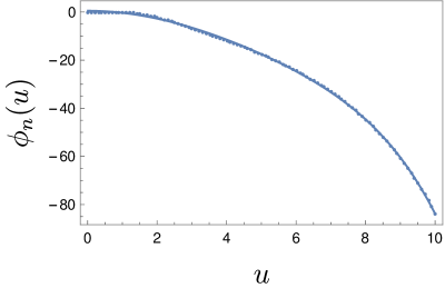
Figure 2: The dotted line shows the dilaton addition obtained by solving numerically Eq. (29). The full line represents a fit to the dilaton addition obtained by the following function: $\phi_{n}(u)\sim a+b~{}u^{3/2}+c~{}u^{2}+d~{}u^{4}+e~{}u^{6}$ whose coefficients are shown in the Appendix A. Here $u=\alpha k^{2}z^{2}$.

Once a solution has been shown to be exist, the equation of motion for the scalar meson is that obtained in Ref. Rinaldi and Vento (2020b) and with the potential shown in Eq. (28) which corresponds to the described truncation of the metric. Let us point out that for the moment being since we are mainly interested in the spectra, the explicit expression of $\phi_{n}$ is not needed once its existence is verified. In closing this section we remark that the philosophy beyond the procedure is to reproduce a phenomenological potential which leads to an excellent description of the spectra despite its simplicity, as will be presented in the next sections. Furthermore, the procedure does not require any new free parameters making as clear as possible the physical interpretation. In fact, the dilaton is the mechanism used in the SW model to describe confinement. On the other hand, the deformation of the metric has been introduced to describe what in the dual QCD sector is an additional interaction of gluons beyond confinement leading to the correct glueball spectra. We recall that we are dealing with $1/N_{c}$ physics. Therefore, if this additional contribution destroys confinement in the meson sector, it cannot be correctly interpreted as a realistic contribution to the SW model providing the correct binding energy for those systems. Therefore, an appealing solution is to modify the dilaton, in the meson sector, to dynamically compensate the metric effects which prevent the binding. The consequent truncation of the exponential up to the third term provides confinement. Thus, such a procedure can be physically interpreted as an attempt to estimate additional gluon effects beyond confinement in the standard SW description of the mesons. As it will be deeply shown later on, the good results, in describing all the spectra, by using only two parameters, suggest that this procedure is appealing and realistic. In closing, let us stress again that despite the dependence of dilaton on the considered systems, as shown in Appendix C, the differential equation for the addition $\phi_{n}$ has the same form for scalar and vector fields. The differences arise due to their AdS mass $M_{5}^{2}R^{2}$ and two calculated coefficients related to their kinematics (see Appendix C for details). Therefore we remark that our procedure does not introduce any new freedom in the model. We conclude that in the GSW model, confinement is determined by the interplay of the glueball dynamics of QCD described by the metric Eq. (1), and confinement described by a well defined dilaton which leads to a phenomenological binding potential.

V.1 The scalar meson with the new dilaton

Motivated by the properties of the new dilaton, $\phi_{0}+\phi_{n}$, we recall here the main outcome of Ref. Rinaldi and Vento (2020b), i.e. the light and heavy meson spectra within the GSW model. As already discussed, the main effect of the correction $\phi_{n}$ is to produce a potential similar to that of Eq. (23) but with the exponential truncated to the third term. The final Schrödinger equation Eq. (23) is shown in terms of the adimensional variable $u=\sqrt{k^{2}/2}\;z$,

$$-\frac{d^{2}\sigma(u)}{du^{2}}+\left(4u^{2}+4+\frac{15}{4u^{2}}-\frac{3}{u^{2}}e^{2\alpha u^{2}}\right)\sigma(u)=\Omega^{2}\sigma(u),$$ (30)

where $\Omega^{2}=(2/k^{2})M^{2}$.

Expanding the exponential up to third order in Eq.(30) we get

$$-\frac{d^{2}\sigma(u)}{du^{2}}+\left((4-6\alpha^{\color[rgb]{0,0,0}2})u^{2}+(4-6\alpha)+\frac{3}{4u^{2}}\right)\sigma(u)=\Omega^{2}\sigma(u).$$ (31)

This equation can be transformed into a Kummer type equation by the change of variables $v=(4-6\alpha^{2})^{1/4}u$

$$-\frac{d^{2}\sigma(v)}{dv^{2}}+\left(v^{2}+\frac{4-6\alpha}{\sqrt{4-6\alpha^{2}}}+\frac{3}{4v^{2}}\right)\sigma(v)=\frac{\Omega^{2}}{\sqrt{4-6\alpha^{2}}}{\color[rgb]{0,0,0}\sigma(v)},$$ (32)

which has an exact spectrum given by

$$\Omega_{n}^{2}=4(n+1)\sqrt{4-6\alpha^{2}}+4-6\alpha,\;n=0,1,2,\ldots.$$ (33)

and the mode functions are

$$\sigma(v)=\mathcal{N}e^{-v^{2}/2}v^{3/2}{{}_{1}F_{1}}(-n,2,v^{2})$$ (34)

where $\mathcal{N}$ is a normalisation factor and ${}_{1}F_{1}$ is a well known hypergeometric function and recall that $v=(4-6\alpha^{2})^{(1/4)}\;u$ where $u=(\sqrt{k^{2}/2}\;z)$. Note that the approximate solution only has bound states for $|\alpha|<\sqrt{2/3}$. The meson modes are functions of $\alpha$. As one can see in the left panel of Fig. 3 a good fit is found for $0.51\leq\alpha\leq 0.59$.

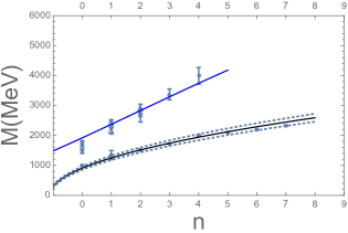
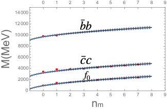
Figure 3: Left panel: GSW fit to the scalar lattice glueball spectrum Morningstar and Peardon (1999); Chen et al. (2006); Lucini et al. (2004) and to the experimental scalar meson spectrum Tanabashi et al. (2018); Zyla et al. (2020) .The larger slope of the glueball spectrum is noticeable. The corresponds to $\alpha k^{2}=(0.37$GeV)² and the values of $\alpha$: $0.55$ (solid) and $0.55\pm 0.04$ (dotted). Right panel: The scalar meson spectrum GSW fit to the data shown for all quark sectors. The light dots represent the scalar meson spectrum experimental data  Tanabashi et al. (2018); Zyla et al. (2020). The curves correspond to Eq. (35) with $C_{c}=2400$ MeV for the $c\bar{c}$ mesons and $C_{b}=8700$ MeV for the $b\bar{b}$ mesons and the values of $\alpha$: $0.55$ (solid) and $0.55\pm 0.04$ (dotted) for all mesons.

V.2 Heavy mesons

In addition in Ref. Rinaldi and Vento (2020b) it has been shown that the GSW can also reproduce the heavy meson spectra by following the procedures developed in Refs. Branz et al. (2010); Kim et al. (2007); Afonin and Pusenkov (2013), i.e. by including in the dynamics the mass of the heavy quarks. Among the different possibilities, we have used the following ansatz:

$$M_{n}=\sqrt{A(\alpha)n+B(\alpha)}+C,$$ (35)

where $C$ is the contribution of the quark masses, thus there will be a $C_{c}$ for the $c\bar{c}$ states and a different one $C_{b}$ for the $b\bar{b}$ states. The comparison between data  Tanabashi et al. (2018); Zyla et al. (2020) and predictions are shown in the right panel of Fig. 3. In order to perform the calculation, the value of $\alpha$ has been kept fixed from that obtained in the analysis of light mesons, i.e. $\alpha=0.55$ (solid) and $\alpha=0.55\pm 0.04$ (dotted). Moreover, $C=0$ for the light quark sector, $C_{c}=2400$ MeV, for the $c\bar{c}$ mesons, and for the $b\bar{b}$ mesons $C_{b}=8700$ MeV. As one can see in the right panel of Fig. 3, the model reproduces the data extremely well. Moreover, one should notice that the additional parameters $C_{c}$ and $C_{b}$ are extremely close to the value of $2m_{c}$ and $2m_{b}$, respectively, as expected. Let us stress that the heavy quark sector has not been considered to estimate the value of $\alpha$. From the present calculations one can conclude that all mesons satisfy approximately the same mass trajectories apart from an overall scale associated with the quark masses and that all the elements in Refs.  Tanabashi et al. (2018); Zyla et al. (2020) suspected of being scalar mesons seem to be scalar mesons, except for some possible mixing with the low lying scalar glueballs, which is not contemplated in this scheme Rinaldi and Vento (2020b). The model has proven to be tremendously predictive. Details on the comparison with data are displayed in Tab. 5. We summarise this section by stating that the GSW model describes well the scalar lattice glueball and the phenomenological scalar meson spectra of QCD with only two parameters, i.e. $\alpha$ and energy scale $\sqrt{\alpha}\,k$ Rinaldi and Vento (2018, 2020b).

light	$f_{0}(500)$	$f_{0}(980)$	$f_{0}(1370)$	$f_{0}(1500)$	$f_{0}(1710)$	$f_{0}(2020)$	$f_{0}(2100)$	$f_{0}(2200)$
$I^{G}(J^{PC})$	$0^{+}(0^{++})$	$0^{+}(0^{++})$	$0^{+}(0^{++})$	$0^{+}(0^{++})$	$0^{+}(0^{++})$	$0^{+}(0^{++})$	$0^{+}(0^{++})$	$0^{+}(0^{++})$
PDG	$475\pm 75$	$990\pm 20$	$1350\pm 150$	$1504\pm 6$	$1723\pm 6$	$1992\pm 16$	$2101\pm 7$	$2189\pm 13$
GSW model Rinaldi and Vento (2020b)		$907\pm 73$	$1248\pm 93$	$1514\pm 109$	$1740\pm 123$	$1941\pm 136$	$2121\pm 147$	$2288\pm 157$
$c\bar{c}$	$\chi_{c0}(1P)$	$\chi_{c0}(3860)$	$X(3915)$	$X(3940)$	$X(4160)$	$X(4350)$	$\chi_{c0}(4500)$	$\chi_{c0}(4700)$
$I^{G}(J^{PC})$	$0^{+}(0^{++})$	$0^{+}(0^{++})$	$0^{+}(0/2^{++})$	$?^{?}(?^{??})$	$?^{?}(?^{??})$	$0^{+}(?^{??})$	$0^{+}(0^{++})$	$0^{+}(0^{++})$
PDG	$3414\pm 0.30$	$3862^{+66}_{-45}$	$3918\pm 1.9$	$3942^{+13}_{-12}$	$4156^{+40}_{-35}$	$4350^{+5.3}_{-5.1}$	$4506^{+42}_{-41}$	$4704^{+24}_{-34}$
GSW model Rinaldi and Vento (2020b)	$3307\pm 73$	$3648\pm 93$	$3914\pm 109$	$4141\pm 123$	$4340\pm 136$	$4521\pm 147$	$4688\pm 157$	$4844\pm 168$
$b\bar{b}$	$\chi_{b0}(1P)$	$\chi_{b0}(1P)$
$I^{G}(J^{PC})$	$0^{+}(0^{++})$	$0^{+}(0^{++})$
PDG	$9859\pm 0.73$	$9912.21\pm 0.57$
GSW model Rinaldi and Vento (2020b)	$9707\pm 73$	$10048\pm 92$

Table 5: Scalar meson spectrum [MeV] from the PDG listings  Tanabashi et al. (2018); Zyla et al. (2020) together with our results for $\alpha=0.55\pm 0.04$ and the energy scale $\sqrt{\alpha}\,k=370$ MeV, see Ref. Rinaldi and Vento (2020b) for details. Notice that in the PDG listings some of the particles are only suspected to be scalars and others need confirmation.

VI The $\rho$ vector meson spectrum

Let us apply the GSW model to the calculation of the spectrum of the vector meson family of the $\rho$. We consider a vector field in the modified $AdS$ space. The respective action Folco Capossoli et al. (2020), modified with the GSW metric, reads,

$$\bar{S}=-\dfrac{1}{2}\int d^{5}x~{}\sqrt{-\bar{g}}~{}e^{\beta_{\rho}k^{2}z^{2}}\left[\dfrac{1}{2}\bar{g}^{MP}\bar{g}^{QN}F_{MN}F_{PQ}+M_{5}^{2}R^{2}\bar{g}^{PM}A_{P}A_{M}\right]~{},$$ (36)

where for the rho meson the AdS mass given by Eq.(24) leads to $M_{5}^{2}R^{2}=0$ since the conformal dimension is $\Delta=3$ and the p-form index $p=1$ Martin Contreras et al. (2020). Since $M_{5}^{2}R^{2}=0$, there is no need to add a correction to the initial dilaton $\phi(z)=\beta_{\rho}k^{2}z^{2}$, in fact, the simplest solution to the relative differential equation, see Appendix B, is $\phi_{n}(z)=0$. Therefore, as previously discussed, if one moves to the standard AdS metric, the action can be rearranged as,

$$\bar{S}=-\dfrac{1}{2}\int d^{5}x~{}\sqrt{-g}~{}e^{k^{2}z^{2}(\beta_{\rho}+\alpha/2)}\left[\dfrac{1}{2}g^{MP}g^{QN}F_{MN}F_{PQ}\right]~{}.$$ (37)

Let us remark that in this case the GSW model is formally equivalent to the SW one because the deformed metric does not affect the EoM since $M_{5}^{2}R^{2}=0$. Nevertheless, we anticipate that the energy scale $k$ will not be considered as a free parameter but instead we will use the value fixed in the scalar sector. As discussed in the previous section, we fix $\beta_{\rho}$ by imposing that the kinematic term in the action is the same as that in the usual SW $AdS$ action, thus $\beta_{\rho}=1+\frac{1}{2}\alpha$. After this choice the action becomes,

$$\bar{S}=-\dfrac{1}{2}\int d^{5}x~{}\sqrt{-g}~{}e^{-k^{2}z^{2}}\left[\dfrac{1}{2}g^{MP}g^{QN}F_{MN}F_{PQ}\right]~{},$$ (38)

which is the same expression used in Ref. Folco Capossoli et al. (2020). Also in this case, an EoM in the Schrödinger form can be found:

$$-\psi^{\prime\prime}(z)+\left[\dfrac{B^{\prime}(z)^{2}}{4}-\dfrac{B^{\prime\prime}(z)}{2}\right]\psi(z)=M^{2}\psi(z)~{}.$$ (39)

By setting $B(z)=k^{2}z^{2}+\log{z}$, the above expression becomes:

$$-\psi^{\prime\prime}(z)+\left(\frac{3}{4z^{2}}+k^{4}z^{2}\right)\psi(z)=M^{2}\psi(z)~{},$$ (40)

This equation can be exactly solved and the spectrum is given by

$$M_{\rho}=2\sqrt{1+n}~{}k~{}.$$ (41)

Due to the fact that the five dimensional mass is zero, this formula coincides with that given in Ref. Karch et al. (2006) however now we have no freedom to fix the parameter $k$ which is given by $k=370/\sqrt{\alpha}$ MeV with $\alpha$ determined from the scalar glueball and meson spectra to be $0.51\leq\alpha\leq 0.59$. One should notice that we can mathematically recover the results of Ref. Folco Capossoli et al. (2020) by setting $\beta_{\rho}=0$ and $\alpha=1$.

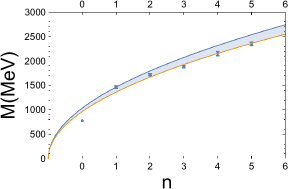
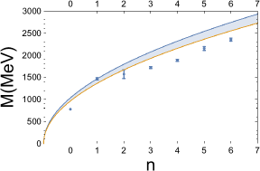
Figure 4: Left: The $\rho$ mass plot as a function of mode number according to the GSW model compared with the data where the experimental $\rho(1570)$ has been excluded following the discussion of the PDG particle listings  Tanabashi et al. (2018); Zyla et al. (2020). Right: the same plot with the $\rho(1570)$ included. The result is not a fit since the parameters have been determined from the scalar mesons and the scalar glueballs.

	$\rho(770)$	$\rho(1450)$	$\rho(1570)$	$\rho(1700)$	$\rho(1900)$	$\rho(2150)$	$\rho(2350)$
PDG	$775.26\pm 0.25$	$1465\pm 25$	$1570\pm 36\pm 62$	$1720\pm 20$	$1885\pm 22$	$2151\pm 42$	$2330\pm 35$
This work	$997\pm 38$	$1411\pm 54$		$1728\pm 66$	$1995\pm 76$	$2231\pm 85$	$2444\pm 94$
Work of Ref. Folco Capossoli et al. (2020)	$868.3$	$1228$	$1504$	$1736.7$	$1941.6$	2127

Table 6: We show the experimental result for the $\rho$ masses in MeV together with the results of our calculation for $\alpha=0.55\pm 0.04$ and $k=370/\sqrt{\alpha}$ MeV. The experimental values were taken from the PDG particle listings  Tanabashi et al. (2018); Zyla et al. (2020). We also report the results obtained by the model of Ref. Folco Capossoli et al. (2020).

The phenomenological $\rho$ spectrum requires some comments before we show our results. The $\rho$ mesons are characterized by $J^{P\,C}=1^{-\,-}$. However, looking deeper into the phenomenological analysis  Tanabashi et al. (2018); Zyla et al. (2020) the $\rho(1570)$ is supposed to be OZI forbidden decay of the $\rho(1700)$ and therefore is not a pure $\rho$ state. As one can see in the left plot of Fig. 4 and Table 6 we get an overall good result for the spectrum. We must stress that our result is not a fit since we have taken the parameters from the scalar sector. In the right panel of of Fig. 4 we include the $\rho(1570)$ as the $n=3$ mode to show that this incorporation distorts completely the agreement. Thus the GSW model predicts that the $\rho=1700$ is the $n=3$ mode and not the $\rho=1570$. Some authors take out the so called D-rho mesons from the S-rho mesons in the mass fit Folco Capossoli et al. (2020). Since the GSW model is well defined in the large $N$ limit, the present approach can not distinguish the above states. Our mode number $n$ acts as a good quantum number and incorporates S and D states. Our result shown in Fig. 4 and Table 6 reproduces all the masses of the rho meson states with the precision required from a large $N$ approximation. The main discrepancy, i.e. the $\rho(770)$, has to do with the observation that the low lying strongly bound states are not so well reproduced in large $N$ QCD.

If one represents $M^{2}$ as a function of $n$ one gets straight lines whose slope is $4k^{2}=4\times 0.37^{2}/\alpha$ which is in the range $1.002\pm 0.072$, included in the universal range $1.25\pm 0.25$ Anisovich et al. (2000). The difference comes again from the discrepancy in the mass of the $\rho(770)$.

VII The $a_{1}$ axial meson spectrum

	$a_{1}(1260)$	$a_{1}(1420)$	$a_{1}(1640)$	$a_{1}(1930)$	$a_{1}(2095)$	$a_{1}(2270)$
PDG & Av	$1230\pm 40$	$1411^{+15}_{-13}$	$1655\pm 16$	$1930^{+19}_{-70}$	$2096^{+17}_{-121}$	$2270^{+55}_{-40}$
This work	833 $\pm 53$	$1235\pm 72$	$1535\pm 87$	$1785\pm 100$	$2005\pm 111$	$2202\pm 122$
Work of Ref. Martin Contreras et al. (2020)	808.1	$1114.7$	$1351.3$	$1558.7$	$1744.3$	$1913.4$

Table 7: We show the experimental result for the $a_{1}$ masses in MeV together with the results of our calculation for $\alpha=0.55\pm 0.04$ and $k=370/\sqrt{\alpha}$ MeV. The three lower masses were taken from the PDG particle listings  Tanabashi et al. (2018); Zyla et al. (2020) and the three higher masses from Ref. Anisovich et al. (2001). A comparison with the results obtained by the model of Ref. Martin Contreras et al. (2020) is also shown.

In the present approach, the only difference between vector mesons and axial-vector mesons due to chiral symmetry breaking is that the latter have $M_{5}^{2}R^{2}\neq 0$, see Ref. He et al. (2010) for details. A mechanism for chiral symmetry breaking can change the mass equation by introducing an anomalous conformal dimension $\Delta_{p}$ Martin Contreras et al. (2020)

$$M_{5}^{2}R^{2}=(\Delta+\Delta_{p}-p)(\Delta+\Delta_{p}+p-4).$$ (42)

$\Delta_{p}=0$ for scalar mesons and vector mesons and turns out to be $\Delta_{p}=-1$ for pseudoscalar mesons and axial vector mesons. Thus $M_{5}^{2}R^{2}=-4$ for pseudoscalars and $M_{5}^{2}R^{2}=-1$ for axial vector mesons. Therefore the EoM for the $a_{1}$ becomes

$$-\psi^{\prime\prime}(z)+\left(\frac{3}{4z^{2}}+k^{4}z^{2}-\frac{e^{\alpha k^{2}z^{2}}}{z^{2}}\right)\psi(z)=M^{2}\psi(z)~{}.$$ (43)

As already discussed several times, such a potential is not binding. Therefore also in this case a modification of the dilaton, $\phi_{n}$, is included so that the effective potential is obtained by expanding the term $e^{\alpha k^{2}z^{2}}$ in the above expression up to the second order. The differential equation for $\phi_{n}$ is explicitly shown in the Appendix B . The corresponding spectrum equation reads:

$$M^{2}=\big{[}4(n+1)\sqrt{1-\alpha^{2}}-\alpha\big{]}k^{2},$$ (44)

which naturally for $\alpha=0$ coincides with the vector meson mass. Using our fixed value $k=370/\sqrt{\alpha}$ MeV and $\alpha=0.55\pm 0.04$ we get the spectrum shown in Fig.5 and Table 7, which is close to the experimental results. Our calculation favors that the $a_{1}(1930),a_{1}(2095)$ and $a_{1}(2270)$, not appearing in the PDG  Tanabashi et al. (2018); Zyla et al. (2020) but shown in Ref. Anisovich et al. (2001), are axial resonances, thus favoring more experimental research in those energy regions. Moreover, in the right panel of Fig. 5, the same data are shown shifted by one unit in $n$. As one can see the agreement of the calculation with data increases. Therefore, in this very first application of the GSW model to the axial vector spectrum, one could propose that the model predicts the existence of a missing ground state with a mass lower then the quoted 1230 MeV.

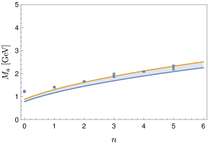
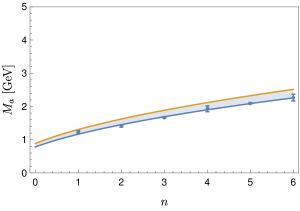
Figure 5: The $a_{1}$ mass plot as a function of mode number according to the GSW model compared with the data. The three lighter $a_{1}$ experimental masses are from Ref. Tanabashi et al. (2018); Zyla et al. (2020), while the three heavier ones have been taken from Ref.Anisovich et al. (2001). The result is not a fit since the parameters have been determined from the scalar mesons and the scalar glueballs. Left panel: calculation vs data. Right panel: same of the left one but data shifted in the $n$ axis by one unity.

VIII Pseudo-scalar mesons

Lastly we will discuss the spectrum of the pseudo-scalar mesons. The EoM is governed by the conformal dimension related to dual field operator of the considered hadron. For a pseudo-scalar meson the study of the conformal dimensions leads to an AdS mass $M_{5}^{2}R^{2}=-4$ Martin Contreras et al. (2020). Thus we are going to consider the spectrum of particles characterized by $J^{PC}=0^{-+}$, which correspond in the spectroscopic notation, previously used, to $J=0$ and $L$=0. In this case the EoM becomes

$$-\frac{d^{2}\psi(z)}{dz^{2}}+\left(k^{4}z^{2}+2k^{2}+\frac{15}{4z^{2}}-\frac{4}{z^{2}}e^{\alpha k^{2}z^{2}}\right)\psi(z)=M^{2}\psi(z).$$ (45)

Since in this approach the pseudo-scalar and scalar mesons are described within the same formalism, the only different is $M_{5}^{2}R^{2}$ and therefore one can add the correction of the dilaton which satisfies Eq. (29). Thus, the truncated potential is recovered. From the phenomenological point of view there are two families of pseudoscalar particles: the $\pi$’s and the $\eta$’s. Let us first study the $\eta$’s.

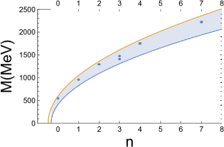
Figure 6: The spectrum of the $\eta$ meson. The upper curve corresponds to $\alpha=0.51$ and the lower curve to $\alpha=0.59$. We have given $\eta(1405)$ and $\eta(1475)$ the same mode number, $n=3$, (see discussion in the text), and we have skipped modes $n=5,6$ since the mass gap between the $\eta(1760)$ and the $\eta(2225)$ is double that of the lower mass $\eta$’s.

VIII.1 The $\eta$ pseudoscalar meson

	$\eta$	$\eta^{\prime}$	$\eta(1295)$	$\eta(1405)$ - $\eta(1475)$	$\eta(1760)$	$\eta(????)$	$\eta(????)$	$\eta(2225)$
PDG	$547.862\pm 0.017$	$957.78\pm 0.06$	$1295\pm 4$	$1408.8\pm 2.0$	$1751\pm 15$			$2221\pm 12$
				$1475\pm 4$
This work	$513\pm 92$	$943\pm 111$	$1231\pm 133$	$1463\pm 151$	$1663\pm 168$	$1842\pm 183$	$2005\pm 198$	$2155\pm 210$

Table 8: We show the experimental results for the $\eta$ masses, in MeV, given by the PDG reviews  Tanabashi et al. (2018); Zyla et al. (2020) together with the results of our calculation. The gaps are introduced in order to respect the mass gaps of the GSW model calculation.

In Fig. 6 we show our calculation where the band characterizes $\alpha=0.55\pm 0.04$. In Table 8 we show the PDG values of the $\eta$ masses  Tanabashi et al. (2018); Zyla et al. (2020) compared with the results of our calculation. It is discussed in PDG review that the $\eta(1405)$ and the $\eta(1475)$ might be the same particle, which is what seems to indicate our calculation. Moreover in the upper mass sector the experimental mass gap becomes larger, which according to the GSW model might indicate that some eta resonances are experimentally missing. In the Table 8 and in Fig. 6 we have left those mode numbers empty between the $\eta(1760)$ and the $\eta(2225)$. If one trusts the results of the calculation, the GSW model predicts the existence of two resonances between the $\eta(1760)$ and the $\eta(2225)$ and that the $\eta(1405)$ and $\eta(1470)$ seem to be the same resonance. From the flavour content it is know that the $\eta$’s have hidden strangeness and therefore corrections associated to the quark mass should be added. Since the strange quark is not too heavy the corrections will be smaller than our theoretical errors. We must stress, once more, that this calculation is not a fit since our parameters were fixed by the scalar spectrum.

VIII.2 The $\pi$ pseudoscalar spectrum

The main difference between the $\eta$ and the $\pi$ is the isospin, however since our model does not take into account Coulomb corrections, the charge-less pions behave very much like the $\eta$ from the point of view of quantum numbers and therefore the spectrum should be the same in our model but it is not so in nature. In fact, there is one main difference, indeed the pion is the Goldstone boson of SU(2) x SU(2) chiral symmetry and this fact is instrumental in giving the lightest pion its low mass. We should therefore implement the spontaneous broken realization of chiral symmetry in the GSW holographic model to reproduce the low mass of the ground state pion. The physics of confinement and chiral symmetry breaking is described by the dilaton  Erlich et al. (2005); Gherghetta et al. (2009); Vega and Cabrera (2016). Therefore, to the present aim, a modification of the dilaton profile function is here proposed to implement the realization of chiral symmetry in a phenomenological way. The dilaton besides the conventional behaviour $\phi_{0}(z)\sim\beta_{s}k^{2}z^{2}$ at large $z$, which determines Regge behaviour, requires a different behaviour at low $z$ to implement chiral symmetry, namely $\varphi(z)\sim\beta^{\prime}k^{2}z^{2}+\mathcal{O}(z^{4})$ , with $\beta^{\prime}<\beta$ Gherghetta et al. (2009). To the present aim, an efficient choice for the dilaton profile function is to promote $\beta$ to be a function of $z$

$$\beta(z)=\beta_{\infty}\tanh{(\gamma z^{4}+\delta)}~{}.$$ (46)

This kind of ansatz has been considered several times in different analyses to implement the chiral symmetry breaking in holographic models, see Refs. Erlich et al. (2005); Gherghetta et al. (2009); Vega and Cabrera (2016). This ansatz leads, as required by chiral symmetry, to,

$$\lim_{z\rightarrow\infty}\beta(z)=\beta_{\infty}~{},$$ (47)

and

$$\lim_{z\rightarrow 0}\beta(z)=\beta_{0}=\beta_{\infty}\tanh{(\delta)}+\mathcal{O}(z^{4})<\beta_{\infty}.$$ (48)

The term $\tanh{(\delta)}$ is therefore related to the realization of chiral symmetry. With this phenomenological input, the dilaton function becomes

$$\phi_{0}(z)=\beta_{\infty}\tanh{(\gamma z^{4}+\delta)}k^{2}z^{2}$$ (49)

with $\beta_{\infty}=\beta_{s}=1+\frac{3}{2}\alpha$ to satisfy the correct large $z$ behaviour once we take into account the effect of the GSW metric. Thus, the large $z$ behaviour, which dominates the spectrum of the higher modes, leads to the Regge behaviour. In the low $z$ region, which is related to the transition region, $\delta$ and $\gamma$, characterise the spontaneous chiral symmetry breaking beyond $\Delta_{p}$, i.e., the effect associated with the bulk 5D mass discussed previously. With this new dilaton, the equations of motion can be generated by using the same strategy previously discussed but by introducing the new dilaton in the functions $B(z)$. As one might expect, the relative potential is more complicated w.r.t. the $\eta$ and other mesons. We again perform an expansion of the exponential to keep the largest binding potential and dismiss the terms which make it not confining. From a phenomenological point of view, one should expect that the value of $\gamma$ depends on the hadron under scrutiny. In particular, in the case of the low mass pion, $\gamma$ must be relatively low so that the transition to the large $z$ limit occurs at higher values. Let us try to fit the low mass pion with the new dilaton. In Fig.7 we show the wave function of a $135$ MeV pion for $\delta=1.5325$ and $\gamma=0.0055$ GeV^-4. The value of $\delta$ has been chosen to have a $n=0$ mode in the approximate well behaved solution. We have kept this value fixed in the non linear full equation and have varied only the $\gamma$ to get a solution as close as possible to the approximate one. The other parameters $\alpha$ and $k$ have been fixed as above.

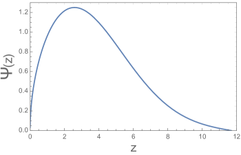
Figure 7: We show the wave function for a $135$ MeV pion with the new dilaton. We have used $\delta=1.5235$ and $\gamma=0.0055$GeV^-4, $\alpha=0.55$ and $k=0.37/\sqrt{\alpha}$ GeV .

In order to calculate the full pion spectrum, one should notice that the excited states, namely $n\geq 1$, are not Goldstone bosons, therefore it is reasonable to assume that the relative EoM should be that described by Eq. (45). In other words, within this prescription, the underline dynamics generating resonances of the pion should be similar to that of the $\eta$ meson. The full pion spectrum is displayed in the Table 9 compared with the PDG data Tanabashi et al. (2018); Zyla et al. (2020). As one might notice, the GSW model, incorporating the chiral symmetry breaking effect in the dilaton profile function, predicts a number of pion states bigger than those experimentally observed. Such a feature is shared with other models Martin Contreras et al. (2020); Gherghetta et al. (2009). However, let us remark that the present experimental results are somehow not conclusive. Indeed, the $\pi(1300)$ has a not well defined mass and a large width (over $200$ MeV), thus it might hide two resonances within its huge width. Moreover, the $\pi(1800)$ has experimental results ranging from $1770$ to $1870$ and also a large width and a complicated two pic structure. In this scenario, the large $N$ approximation, encoded in approach here proposed, is predicting states that could be observed once the experimental region is cleared up.

Finally one may wonder if the new dilaton will change the $\eta$ spectrum, previously described. Let us show that this is not the case. In Fig. 8, the wave functions of the first two $\eta$ modes, for the masses determined above $512$ and $943$ MeV with the new dilaton (solid) and the old dilaton (dashed), are shown. One sees that keeping fixed $\delta=1.5235$, which should be the same for all particles, and letting $\gamma$ grow up to $\gamma\sim 1.0$, to displace the transition region to lower $z$ values, one obtains exactly the same spectrum and almost exactly the same wave functions. For larger values of $\gamma$ the resemblance of the wave functions is even greater, but then we are mathematically approximating the old dilaton mode. For higher modes, the required value of $\gamma$, for almost equality, can be even lower since the $z^{4}$ term dominates the $\beta(z)$ function. For values as low as $\gamma=0.2$, the wave functions are not so close but still very similar. Furthermore, as a cross check of the procedure to provide a binding potential, in Fig. 9 it has been numerically shown that the correction to the dilaton applied to the $\eta$ case is very close to that needed for the $\pi$ case. Such a feature reflects that also in the GSW model, the $\chi$sb can be described by a new dilaton $\phi_{0}$ (49), while the truncation of the metric effect in the potential can still be obtained by means of corrections that for the pseudo-scalar systems are very similar.

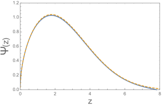
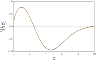
Figure 8: The wave functions of the $\eta$ (left) and $\eta^{\prime}$ (right) with the new dilaton (solid), old dilaton (dashed). The new dilaton has been calculated with $\alpha=0.55$, $\delta=1.5235$,$\gamma=1.0$ and $k=0.37/\sqrt{\alpha}$ GeV. The masses of the etas for the two dilaton calculations are identical $m_{\eta}=512$ MeV and $m_{\eta^{\prime}}=943$ MeV.

	$\pi^{0}$		$\pi(1300)$			$\pi(1800)$
PDG	$134.9768\pm 0.0005$		$1300\pm 100$			$1819\pm 10$
This work	$135$	$943\pm 111$	$1231\pm 133$	$1463\pm 151$	$1663\pm 168$	$1842\pm 183$

Table 9: We show the experimental result for the $\pi$ masses given by the PDG particle listings Tanabashi et al. (2018); Zyla et al. (2020) together with the results of our calculation. We have used the $\pi^{0}$ mass to fix the value of $\delta=1.5235$. Our errors are again associated with the error in $\alpha=0.55\pm 0.04$. The masses are as always in MeV.

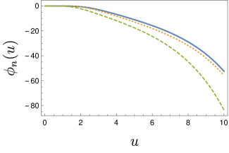
Figure 9: The dilaton addition $\phi_{n}$ for the pseudo-scalar systems, see Appendix A. Full fine: the calculation for the pion with the initial dilaton $\phi_{0}$ of Eq. (49). Dotted line: results obtained for the $\eta$ meson with the initial dilaton $\phi_{0}=\beta_{s}k^{2}z^{2}$. Dashed line: the same for the scalar meson. Here $u=\alpha k^{2}z^{2}$.

IX Conclusions

In the present investigation, a phenomenological analysis of the glueball and meson spectra within the GSW model is provided. This approach is based on the assumption that the lowest scalar glueball is associated to a graviton propagating in a deformed $AdS_{5}$ space. We saw in the past that the metric is fundamental in providing a good representation of the experimental data with only one parameter, and in so doing we determined the energy scale $k$ of the model. No approximation to the metric leads to a reasonable result, the graviton requires of the full power of the metric to produce the adequate experimental slope and, in turn, to describe the correspondence to the confinement mechanism. The next step was to fit the scalar mesons within the same model. In this case the $AdS_{5}$ mass is negative and therefore the corresponding mode potential does not bind. In order to make the potential confining we had to truncate the exponential at third term. After doing so we obtain an excellent fit to the light meson spectrum with only one additional parameter associated with the strength of the metric $\alpha$. With these two parameters fixed we have proceeded to describe the whole glueball and light meson spectrum. In all fits of glueballs, use has been made of the full metric since the corresponding $AdS_{5}$ masses are positive. On the other hand, for all mesons, except for the $\rho$, whose $AdS_{5}$ mass is zero, we had to truncate the exponential metric at the third term to get a binding potential. With this procedure we have reproduced quite well the mass spectra of the $\rho$, the $a_{1}$, the $\eta$ and the pion. While for the ground state pion a modification of the dilaton profile function is required to implement the chiral symmetry breaking, for all the other hadrons, the masses have been calculated without any fit of the model parameters, which are only two, $k$ and $\alpha$, which were fixed by the scalar glueball and light scalar meson spectra. Such feature underlines the predictive power of the proposed model in describing the hadron masses. We recall that the model is also able to fit well the heavy scalar meson spectra. We can conclude after this phenomenological analysis that the GSW model provides a good description of the spectra of the axial and vector mesons, high spin glueballs and pseudo-scalar mesons and even heavy mesons with very few parameters. Moreover, the model also predicts the existence of further states not yet observed probably due to the present experimental accuracy.

The success of this phenomenological meson potential has led us to investigate how the exponential metric is related to it. We have proven that a modification in the dilaton field is able to generate the phenomenological potential from the full metric. The proof is based on the construction of a differential equation for the dilaton field which relates the initial full potential with the phenomenological potential. We have shown that in our case, for all the mesons studied, the differential equation is solvable and moreover the new dilaton introduces no new parameters since it is defined exclusively by the metric parameters and the corresponding AdS mass. This new dilaton represents additional QCD interactions modifying, in the case of the mesons, the confining mechanism of glueballs.

We have compared the graviton solution for the glueballs, which described the scalar and tensor glueball spectrum with the $J=0$ and $J=2$ glueball field solutions. We have seen that the degeneracy between scalars and glueballs of the former is instrumental in describing the spectra with only one energy scale. The field solutions require different energy scales for the $J=0$ and $J=2$ solutions since the one that fits the scalars leads to extremely heavy tensors, and the one that fits the tensor to extremely light scalars. The graviton seems to be a necessary ingredient of AdS/QCD and the implications of this fact on QCD have to be understood. For the higher $J$ glueballs the field approximation is adequate and it has allowed us to calculate successfully the Regge trajectories of the even and odd high spin glueballs. The scalar glueball and the pion escape this scheme. The former requires a graviton propagating in a deformed $AdS$ space and the latter a sophisticated dilaton. Clearly this might be associated in QCD with the fact that the ground state scalar glueball is associated with the $\sigma$ particle in some schemes and the pion with the Goldstone boson of spontaneously broken chiral symmetry.

One should notice that the GSW model, like other phenomenological approaches based on the the AdS/CFT correspondence, is realized in the large $N$ approximation. Therefore, one might expect higher order corrections to be required for precision calculations, which are beyond the aim of the present investigation. Finally let us conclude by remarking the surprising capability of the model in reproducing basic features of many different hadronic systems without invoking a large number of parameters and therefore unveiling a relevant predicting power that could be used in future analyses.

X Acknowledgements

This work was supported, in part by the STRONG-2020 project of the European Unions Horizon 2020 research and innovation programme under grant agreement No 824093. This work was also supported in part by MICINN, AEI and UE FEDER under contract PID2019-105439-GB-C21.

Appendix A The dilaton differential equation for the scalar and pseudo-scalar fields

In this appendix details on the differential equation (29) will be provided. In particular, since for the pion the initial dilaton ($\phi$) must be properly chosen in order to introduce $\chi$sb into the model, here we provide the general differential equation that the dilaton addition ($\phi_{n}$) must satisfy to generate a binding potential where the metric effects are encoded in the truncated expansion of $e^{\alpha k^{2}z^{2}}$. Let us start again with the full general action for a scalar field:

$$\bar{S}=\int d^{5}x~{}\sqrt{-g}e^{-\phi(z)+\frac{3}{2}\alpha k^{2}z^{2}-\phi_{n}(z)}\Big{[}g^{MN}\partial_{M}S(x)\partial_{N}S(x)+e^{\alpha k^{2}z^{2}}M_{5}^{2}R^{2}S^{2}(x)\Big{]}~{},$$ (50)

where we recall that for $\phi(z)=k^{2}z^{2}\beta_{s}$ and $\beta_{s}=1+\frac{3}{2}\alpha$ we get the usual result Eq. (25) and of Ref. Rinaldi and Vento (2020b). From the Euler-Lagrange equation and by properly choosing a functional form the field $S(x)$, a Schrödinger equation can be obtained,

$$-\psi^{\prime\prime}(z)+V_{s}(z)\psi(z)=M^{2}\psi(z)~{},$$ (51)

where the potential $V_{s}(z)=\tilde{V}_{s}(z)/(4z^{2})$ and,

$$\tilde{V}_{s}(z) =4e^{\alpha k^{2}z^{2}}M_{5}^{2}+3\Big{[}5+\alpha k^{2}z^{2}\ (-4+3\alpha k^{2}z^{2})\Big{]}+$$ (52)

$$+z\Big{\{}z\phi^{\prime}(z)^{2}+(6-6\alpha k^{2}z^{2})\ \phi_{n}^{\prime}(z)+z\phi_{n}^{\prime}(z)^{2}+\phi^{\prime}(z)\big{[}6-6\alpha k^{2}z^{2}+2z\phi_{n}^{\prime}(z)\big{]}-2z\big{[}\phi^{\prime\prime}(z)+\phi_{n}^{\prime\prime}(z)\big{]}\Big{\}}~{}.$$

The equivalent quantity obtained for $\phi_{n}=0$ and $\phi=k^{2}z^{2}(1+\frac{3}{2}\alpha)$ becomes  Rinaldi and Vento (2020b),

$$\tilde{V}_{s}^{o}(z)=15+4M_{5}^{2}R^{2}e^{\alpha k^{2}z^{2}}+8k^{2}z^{2}+4k^{4}z^{4}~{},$$ (53)

Moreover, the binding potential, needed to reproduce the scalar and pseudo-scalar spectra previously discussed, must be obtained by setting $\phi_{n}=0$ and by expanding the exponential term $e^{\alpha k^{2}z^{2}}$ up to the third term:

$$\tilde{V}_{s}^{a}(z) =4(1+\alpha k^{2}z^{2}+\frac{1}{2}\alpha^{2}k^{4}z^{4})M_{5}^{2}+3\Big{[}5+\alpha k^{2}z^{2}\ (-4+3\alpha k^{2}z^{2})\Big{]}+$$ (54)

$$+z\Big{\{}\phi^{\prime}(z)\big{[}6-6\alpha k^{2}z^{2}+2z\big{]}-2z\phi^{\prime\prime}(z)\Big{\}}~{}.$$

Therefore, the differential equation, that the correction dilaton $\phi_{n}$ must satisfy to move from the general potential Eq. (52) to the expression Eq. (54) is,

$$\tilde{V}_{s}(z)-\tilde{V}_{s}^{a}(z)=4M_{5}^{2}R^{2}\Big{[}e^{\alpha k^{2}z^{2}}-1-\alpha k^{2}z^{2}-\frac{1}{2}\alpha^{2}k^{4}z^{4}\Big{]}+z\Big{[}\phi_{n}^{\prime}(z)\big{(}6-6\alpha k^{2}z^{2}+2z\phi^{\prime}(z)+z\phi_{n}^{\prime}(z)\Big{)}-2z\phi_{n}^{\prime\prime}(z)\Big{]}=0~{}.$$ (55)

The above equation can be simplified to:

$$-\frac{\phi^{\prime\prime}_{n}(z)}{2}+\frac{\phi^{\prime}_{n}(z)^{2}}{4}+\phi^{\prime}_{n}(z)\left(\frac{3}{2z}-\frac{3}{2}\alpha k^{2}z+\frac{1}{2}\phi^{\prime}_{n}(z)\right)+\frac{M_{5}^{2}R^{2}}{z^{2}}\left(e^{\alpha k^{2}z^{2}}-1-\alpha k^{2}z^{2}-\frac{1}{2}\alpha^{2}k^{4}z^{4}\right)=0~{}.$$ (56)

As one can see this equation directly depend on the old initial dilaton $\phi$, therefore such a procedure can be applied in the scalar and pseudo-scalar ($\eta$ and $\pi$) mesons. In the case of scalar meson and $\eta$, $\phi(z)=k^{2}z^{2}(1+\frac{3}{2}\alpha)$ one gets:

$$-\frac{\phi^{\prime\prime}_{n}(z)}{2}+\frac{\phi^{\prime}_{n}(z)^{2}}{4}+\phi^{\prime}_{n}(z)\left(\frac{3}{2z}+k^{2}z\right)+\frac{M_{5}^{2}R^{2}}{z^{2}}\left(e^{\alpha k^{2}z^{2}}-1-\alpha k^{2}z^{2}-\frac{1}{2}\alpha^{2}k^{4}z^{4}\right)=0~{}.$$ (57)

The numerical solution has been used to fit $\phi_{n}$ as a polynomial function of $u=\alpha k^{2}z^{2}$:

$$\phi_{n}(u)\sim 0.507286-0.035493u^{1.5}-0.800325u^{2}+0.0052429u^{4}-0.0000556475u^{6}~{}.$$ (58)

Appendix B The dilaton differential equation for the vector field

The same procedure can be extended to vector fields. In this case dilatons describing chiral symmetry breaking are not considered in the analysis. We show the differential equation for $\phi_{n}$ given $\phi_{0}=\beta_{\rho}k^{2}z^{2}$ where $\beta_{\rho}=1+\frac{1}{2}\alpha$.

In this case,

$$\bar{S}_{V}=-\frac{1}{2}\int d^{5}x\sqrt{-g}e^{-k^{2}z^{2}-\phi_{n}}\left[\frac{1}{2}g^{MP}g^{QN}F_{MN}F^{PQ}+M_{5}^{2}R^{2}g^{PM}A_{P}A_{M}e^{\alpha k^{2}z^{2}}\right]~{}.$$ (59)

From the EoM one can derive the potential:

$$V_{v}(z) =\left[\frac{B^{\prime}(z)^{2}}{4}-\frac{B^{\prime\prime}(z)}{2}+\frac{M_{5}^{2}R^{2}}{z^{2}}e^{\alpha k^{2}z^{2}}\right]$$ (60)

$$=-\frac{\phi_{n}^{\prime\prime}(z)}{2}+\frac{\phi_{n}^{\prime}(z)^{2}}{4}+\phi_{n}^{\prime}(z)\left(\frac{1}{2z}-k^{2}z\right)+k^{4}z^{2}+\frac{3}{4z^{2}}+\frac{M_{5}^{2}R^{2}}{z^{2}}e^{\alpha k^{2}z^{2}}~{},$$

where here $B(z)=\log(z)+\phi_{n}(z)-k^{2}z^{2}$. Also in this case, the approximated potential $V_{v}^{a}$ is obtained for $\phi_{n}=0$ and by expanding $e^{\alpha k^{2}z^{2}}$ up to the third term. The phenomenological potential is,

$$V_{v}^{a}(z)=k^{4}z^{2}+\frac{3}{4z^{2}}+\frac{M_{5}^{2}R^{2}}{z^{2}}(1+\alpha k^{2}z^{2}+\frac{1}{2}\alpha^{2}k^{4}z^{4})~{},$$ (61)

therefore the differential equation reads,

$$V_{v}(z)-V_{v}^{a}(z)=-\frac{\phi_{n}^{\prime\prime}(z)}{2}+\frac{\phi_{n}^{\prime}(z)^{2}}{4}+\phi_{n}^{\prime}(z)\left(\frac{1}{2z}-k^{2}z\right)+\frac{M_{5}^{2}R^{2}}{z^{2}}\left(e^{\alpha k^{2}z^{2}}-1-\alpha k^{2}z^{2}-\frac{1}{2}\alpha^{2}k^{4}z^{4}\right)=0.$$ (62)

Appendix C The general dilaton differential equation for $\phi(z)=\beta k^{2}z^{2}$

Due to the similarities between Eqs. (57, 62), we show here that the although the dilaton expression would explicitly depend on the kind of meson (scalar or vector), no free parameter are involved and the differential equation can be written through a general expression:

$$-\frac{\phi_{n,I}^{{}^{\prime\prime}}(z)}{2}+\frac{\phi_{n,I}^{\prime}(z)^{2}}{4}+\phi_{n,I}^{\prime}(z)\left(\frac{A_{I}}{2z}+B_{I}k^{2}z\right)+\frac{M_{5}^{2}R^{2}}{z^{2}}\left(e^{\alpha k^{2}z^{2}}-1-\alpha k^{2}z^{2}-\frac{1}{2}\alpha^{2}k^{4}z^{4}\right)=0~{},$$ (63)

where for the scalar we have $I=s,~{}A_{s}=3,~{}B_{s}=1$ and for the vector $I=v,~{}A_{v}=1,~{}B_{v}=-1$.

*

References

- Maldacena (1999) J. M. Maldacena, Int. J. Theor. Phys. 38, 1113 (1999), [Adv. Theor. Math. Phys.2,231(1998)], arXiv:hep-th/9711200 [hep-th] .
- Witten (1998) E. Witten, Adv. Theor. Math. Phys. 2, 505 (1998), arXiv:hep-th/9803131 [hep-th] .
- Fritzsch et al. (1973) H. Fritzsch, M. Gell-Mann, and H. Leutwyler, Phys. Lett. 47B, 365 (1973).
- Fritzsch and Minkowski (1975) H. Fritzsch and P. Minkowski, Phys. Lett. 56B, 69 (1975).
- Vento (2017) V. Vento, Eur. Phys. J. A53, 185 (2017), arXiv:1706.06811 [hep-ph] .
- Rinaldi and Vento (2018) M. Rinaldi and V. Vento, Eur. Phys. J. A54, 151 (2018), arXiv:1710.09225 [hep-ph] .
- Polchinski and Strassler (2000) J. Polchinski and M. J. Strassler, (2000), arXiv:hep-th/0003136 [hep-th] .
- Brodsky and de Téramond (2004) S. J. Brodsky and G. F. de Téramond, Phys. Lett. B582, 211 (2004), arXiv:hep-th/0310227 [hep-th] .
- Da Rold and Pomarol (2005) L. Da Rold and A. Pomarol, Nucl. Phys. B721, 79 (2005), arXiv:hep-ph/0501218 [hep-ph] .
- Karch et al. (2006) A. Karch, E. Katz, D. T. Son, and M. A. Stephanov, Phys. Rev. D74, 015005 (2006), arXiv:hep-ph/0602229 [hep-ph] .
- Erlich et al. (2005) J. Erlich, E. Katz, D. T. Son, and M. A. Stephanov, Phys. Rev. Lett. 95, 261602 (2005), arXiv:hep-ph/0501128 [hep-ph] .
- Colangelo et al. (2008) P. Colangelo, F. De Fazio, F. Giannuzzi, F. Jugeau, and S. Nicotri, Phys. Rev. D78, 055009 (2008), arXiv:0807.1054 [hep-ph] .
- de Teramond and Brodsky (2005) G. F. de Teramond and S. J. Brodsky, Phys. Rev. Lett. 94, 201601 (2005), arXiv:hep-th/0501022 [hep-th] .
- Colangelo et al. (2007) P. Colangelo, F. De Fazio, F. Jugeau, and S. Nicotri, Phys. Lett. B652, 73 (2007), arXiv:hep-ph/0703316 [hep-ph] .
- Folco Capossoli and Boschi-Filho (2016) E. Folco Capossoli and H. Boschi-Filho, Phys. Lett. B753, 419 (2016), arXiv:1510.03372 [hep-ph] .
- Rinaldi (2017) M. Rinaldi, Phys. Lett. B771, 563 (2017), arXiv:1703.00348 [hep-ph] .
- Bacchetta et al. (2017) A. Bacchetta, S. Cotogno, and B. Pasquini, Phys. Lett. B771, 546 (2017), arXiv:1703.07669 [hep-ph] .
- de Teramond et al. (2018) G. F. de Teramond, T. Liu, R. S. Sufian, H. G. Dosch, S. J. Brodsky, and A. Deur (HLFHS), Phys. Rev. Lett. 120, 182001 (2018), arXiv:1801.09154 [hep-ph] .
- Afonin and Pusenkov (2013) S. S. Afonin and I. V. Pusenkov, Phys. Lett. B726, 283 (2013), arXiv:1306.3948 [hep-ph] .
- Rinaldi and Vento (2020a) M. Rinaldi and V. Vento, J. Phys. G47, 055104 (2020a), arXiv:1803.05738 [hep-ph] .
- Rinaldi and Vento (2020b) M. Rinaldi and V. Vento, J. Phys. G47, 125003 (2020b), arXiv:2002.11720 [hep-ph] .
- Morningstar and Peardon (1999) C. J. Morningstar and M. J. Peardon, Phys. Rev. D60, 034509 (1999), arXiv:hep-lat/9901004 [hep-lat] .
- Chen et al. (2006) Y. Chen et al., Phys. Rev. D73, 014516 (2006), arXiv:hep-lat/0510074 [hep-lat] .
- Lucini et al. (2004) B. Lucini, M. Teper, and U. Wenger, JHEP 06, 012 (2004), arXiv:hep-lat/0404008 [hep-lat] .
- Vega and Cabrera (2016) A. Vega and P. Cabrera, Phys. Rev. D93, 114026 (2016), arXiv:1601.05999 [hep-ph] .
- Akutagawa et al. (2020) T. Akutagawa, K. Hashimoto, and T. Sumimoto, Phys. Rev. D102, 026020 (2020), arXiv:2005.02636 [hep-th] .
- Gutsche et al. (2019) T. Gutsche, V. E. Lyubovitskij, I. Schmidt, and A. Y. Trifonov, Phys. Rev. D99, 054030 (2019), arXiv:1902.01312 [hep-ph] .
- Klebanov and Maldacena (2004) I. R. Klebanov and J. M. Maldacena, Int. J. Mod. Phys. A19, 5003 (2004), arXiv:hep-th/0409133 [hep-th] .
- Martin Contreras and Vega (2020) M. A. Martin Contreras and A. Vega, Phys. Rev. D101, 046009 (2020), arXiv:1910.10922 [hep-th] .
- Folco Capossoli et al. (2020) E. Folco Capossoli, M. A. Martín Contreras, D. Li, A. Vega, and H. Boschi-Filho, Chin. Phys. C44, 064104 (2020), arXiv:1903.06269 [hep-ph] .
- Bernardini et al. (2017) A. E. Bernardini, N. R. F. Braga, and R. da Rocha, Phys. Lett. B765, 81 (2017), arXiv:1609.01258 [hep-th] .
- Li and Huang (2013) D. Li and M. Huang, JHEP 11, 088 (2013), arXiv:1303.6929 [hep-ph] .
- Sarantsev et al. (2021) A. V. Sarantsev, I. Denisenko, U. Thoma, and E. Klempt, Phys. Lett. B 816, 136227 (2021), arXiv:2103.09680 [hep-ph] .
- Klempt (2021) E. Klempt, (2021), arXiv:2104.09922 [hep-ph] .
- Boschi-Filho et al. (2006) H. Boschi-Filho, N. R. F. Braga, and H. L. Carrion, Phys. Rev. D73, 047901 (2006), arXiv:hep-th/0507063 [hep-th] .
- Meyer (2004) H. B. Meyer, Glueball regge trajectories, Ph.D. thesis, Oxford U. (2004), arXiv:hep-lat/0508002 [hep-lat] .
- Gregory et al. (2012) E. Gregory, A. Irving, B. Lucini, C. McNeile, A. Rago, C. Richards, and E. Rinaldi, JHEP 10, 170 (2012), arXiv:1208.1858 [hep-lat] .
- Llanes-Estrada et al. (2006) F. J. Llanes-Estrada, P. Bicudo, and S. R. Cotanch, Phys. Rev. Lett. 96, 081601 (2006), arXiv:hep-ph/0507205 [hep-ph] .
- Mathieu et al. (2008a) V. Mathieu, C. Semay, and B. Silvestre-Brac, Phys. Rev. D77, 094009 (2008a), arXiv:0803.0815 [hep-ph] .
- Szanyi et al. (2020) I. Szanyi, L. Jenkovszky, R. Schicker, and V. Svintozelskyi, Nucl. Phys. A998, 121728 (2020), arXiv:1910.02494 [hep-ph] .
- Szczepaniak and Swanson (2003) A. P. Szczepaniak and E. S. Swanson, Phys. Lett. B577, 61 (2003), arXiv:hep-ph/0308268 [hep-ph] .
- Mathieu et al. (2008b) V. Mathieu, F. Buisseret, and C. Semay, Phys. Rev. D77, 114022 (2008b), arXiv:0802.0088 [hep-ph] .
- Landshoff (2001) P. V. Landshoff, in Elastic and diffractive scattering. Proceedings, 9th Blois Workshop, Pruhonice, Czech Republic, June 9-15, 2001 (2001) pp. 161–171, arXiv:hep-ph/0108156 [hep-ph] .
- Meyer and Teper (2005) H. B. Meyer and M. J. Teper, Phys. Lett. B605, 344 (2005), arXiv:hep-ph/0409183 [hep-ph] .
- Martin Contreras et al. (2020) M. A. Martin Contreras, A. Vega, and S. Cortes, Chin. J. Phys. 66, 715 (2020), arXiv:1811.10731 [hep-ph] .
- Tanabashi et al. (2018) M. Tanabashi et al. (Particle Data Group), Phys. Rev. D98, 030001 (2018).
- Zyla et al. (2020) P. A. Zyla et al. (Particle Data Group), PTEP 2020, 083C01 (2020).
- Branz et al. (2010) T. Branz, T. Gutsche, V. E. Lyubovitskij, I. Schmidt, and A. Vega, Phys. Rev. D82, 074022 (2010), arXiv:1008.0268 [hep-ph] .
- Kim et al. (2007) Y. Kim, J.-P. Lee, and S. H. Lee, Phys. Rev. D75, 114008 (2007), arXiv:hep-ph/0703172 [HEP-PH] .
- Anisovich et al. (2000) A. V. Anisovich, V. V. Anisovich, and A. V. Sarantsev, Phys. Rev. D62, 051502 (2000), arXiv:hep-ph/0003113 [hep-ph] .
- Anisovich et al. (2001) A. V. Anisovich, C. A. Baker, C. J. Batty, D. V. Bugg, V. A. Nikonov, A. V. Sarantsev, V. V. Sarantsev, and B. S. Zou, Phys. Lett. B517, 261 (2001), arXiv:1110.0278 [hep-ex] .
- He et al. (2010) S. He, M. Huang, Q.-S. Yan, and Y. Yang, Eur. Phys. J. C66, 187 (2010), arXiv:0710.0988 [hep-ph] .
- Gherghetta et al. (2009) T. Gherghetta, J. I. Kapusta, and T. M. Kelley, Phys. Rev. D79, 076003 (2009), arXiv:0902.1998 [hep-ph] .
*