A New Approach to Probe Non-Standard Interactions in Atmospheric Neutrino Experiments

Abstract

We propose a new approach to explore the neutral-current non-standard neutrino interactions (NSI) in atmospheric neutrino experiments using oscillation dips and valleys in reconstructed muon observables, at a detector like ICAL that can identify the muon charge. We focus on the flavor-changing NSI parameter $\varepsilon_{\mu\tau}$, which has the maximum impact on the muon survival probability in these experiments. We show that non-zero $\varepsilon_{\mu\tau}$ shifts the oscillation dip locations in $L/E$ distributions of the up/down event ratios of reconstructed $\mu^{-}$ and $\mu^{+}$ in opposite directions. We introduce a new variable $\Delta d$ representing the difference of dip locations in $\mu^{-}$ and $\mu^{+}$, which is sensitive to the magnitude as well as the sign of $\varepsilon_{\mu\tau}$, and is independent of the value of $\Delta m^{2}_{32}$. We further note that the oscillation valley in the ($E$, $\cos\theta$) plane of the reconstructed muon observables bends in the presence of NSI, its curvature having opposite signs for $\mu^{-}$ and $\mu^{+}$. We demonstrate the identification of NSI with this curvature, which is feasible for detectors like ICAL having excellent muon energy and direction resolutions. We illustrate how the measurement of contrast in the curvatures of valleys in $\mu^{-}$ and $\mu^{+}$ can be used to estimate $\varepsilon_{\mu\tau}$. Using these proposed oscillation dip and valley measurements, the achievable precision on $|\varepsilon_{\mu\tau}|$ at 90% C.L. is about 2% with 500 kt$\cdot$yr exposure. The effects of statistical fluctuations, systematic errors, and uncertainties in oscillation parameters have been incorporated using multiple sets of simulated data. Our method would provide a direct and robust measurement of $\varepsilon_{\mu\tau}$ in the multi-GeV energy range.

1 Introduction and Motivation

The phenomenon of neutrino oscillations has now been well-established, from measurements at the solar, atmospheric, reactor as well as accelerator experiments with short and long baselines Zyla:2020zbs . Neutrino oscillations are the consequences of mixing among different neutrino flavors and non-degenerate values of neutrino masses, with at least two neutrino masses nonzero. However, neutrinos are massless in the Standard Model (SM) of particle physics, and therefore, physics beyond the SM (BSM) is needed to accommodate nonzero neutrino masses and mixing. Many models of BSM physics suggest new non-standard interactions (NSI) of neutrinos Wolfenstein:1977ue , which may affect neutrino production, propagation, and detection in a given experiment. The possible impact of these NSI at neutrino oscillation experiments have been studied extensively, for example see Refs. Valle:1987gv ; Guzzo:1991hi ; Guzzo:2000kx ; Huber:2001zw ; Gago:2001si ; Escrihuela:2011cf ; GonzalezGarcia:2011my ; Ohlsson:2012kf ; Gonzalez-Garcia:2013usa ; Farzan:2017xzy ; Miranda:2015dra ; Dev:2019anc . In this paper, we propose a new method for identifying NSI at atmospheric neutrino experiments which can reconstruct the energy, direction, as well as charge of the muons produced in the detector due to charged-current interactions of $\nu_{\mu}$ and $\bar{\nu}_{\mu}$.

We shall focus on the neutral-current NSI, which may be described at low energies via effective four-fermion dimension-six operators as Wolfenstein:1977ue

$${\mathcal{L}}_{\rm{NC-NSI}}=-2\sqrt{2}\,G_{F}\,\varepsilon^{f}_{\alpha\beta,C}\,(\bar{\nu}_{\alpha}\gamma^{\rho}P_{L}\nu_{\beta})\,(\bar{f}\gamma_{\rho}P_{C}f)\,,$$ (1)

where $G_{F}$ is the Fermi constant. The dimensionless parameters $\varepsilon^{f}_{\alpha\beta,C}$ describe the strength of NSI, where the superscript $f\in\{e,u,d\}$ denotes the matter fermions ($e$: electron, $u$: up-quark, $d$: down-quark), and the indices $\alpha,\beta\in\{e,\mu,\tau\}$ refer to the neutrino flavors. The subscript $C\in\{L,R\}$ represents the chiral projection operator $P_{L}=(1-\gamma_{5})/2$ or $P_{R}=(1+\gamma_{5})/2$. The hermiticity of the interactions demands $\varepsilon^{f}_{\beta\alpha,C}=(\varepsilon^{f}_{\alpha\beta,C})^{*}$.

The effective NSI parameter relevant for the neutrino propagation through matter is

$$\varepsilon_{\alpha\beta}\equiv\sum_{f=e,u,d}\left(\varepsilon_{\alpha\beta}^{fL}+\varepsilon_{\alpha\beta}^{fR}\right)\,\,\frac{N_{f}}{N_{e}}\equiv\sum_{f=e,u,d}\varepsilon_{\alpha\beta}^{f}\,\,\frac{N_{f}}{N_{e}}\,,$$ (2)

where $N_{f}$ is the number density of fermion $f$. In the approximation of a neutral and isoscalar Earth, the number densities of electrons, protons, and neutrons are identical, which implies $N_{u}\approx N_{d}\approx 3N_{e}$. Thus,

$$\varepsilon_{\alpha\beta}\approx\varepsilon^{e}_{\alpha\beta}+3\,\varepsilon^{u}_{\alpha\beta}+3\,\varepsilon^{d}_{\alpha\beta}\,.$$ (3)

In the presence of NSI, the modified effective Hamiltonian for neutrino propagation through matter is

$$H_{\rm eff}=\frac{1}{2E}\,U\left(\begin{array}[]{ccc}0&0&0\\ 0&\Delta m^{2}_{21}&0\\ 0&0&\Delta m^{2}_{31}\end{array}\right)U^{\dagger}+V_{\rm CC}\left(\begin{array}[]{ccc}1+\varepsilon_{ee}&\varepsilon_{e\mu}&\varepsilon_{e\tau}\\ \varepsilon_{e\mu}^{*}&\varepsilon_{\mu\mu}&\varepsilon_{\mu\tau}\\ \varepsilon_{e\tau}^{*}&\varepsilon_{\mu\tau}^{*}&\varepsilon_{\tau\tau}\end{array}\right)\,,$$ (4)

where $U$ is the Pontecorvo-Maki-Nakagawa-Sakata (PMNS) matrix that parametrizes neutrino mixing, and $\Delta m^{2}_{ij}\equiv m_{i}^{2}-m_{j}^{2}$ are the mass-squared differences. The quantity $V_{\rm CC}\equiv\sqrt{2}G_{F}N_{e}$ is the effective matter potential due to the coherent elastic forward scattering of neutrinos with electrons inside the medium via the SM gauge boson $W$. Thus, the effective potential due to NSI would be ${(V_{\rm NSI})}_{\alpha\beta}=\sqrt{2}G_{F}N_{e}\,\varepsilon_{\alpha\beta}$. For antineutrinos, $V_{\rm CC}\rightarrow-V_{\rm CC}$, $U\rightarrow U^{*}$, and $\varepsilon_{\alpha\beta}\to\varepsilon_{\alpha\beta}^{*}$.

In the present study, we suggest a novel approach to unravel the presence of flavor-changing neutral-current NSI parameter $\varepsilon_{\mu\tau}$, via its effect on the propagation of multi-GeV atmospheric neutrinos and antineutrinos through Earth matter. We choose $\varepsilon_{\mu\tau}$ as the NSI parameter to focus on, since it can significantly affect the evolution of the mixing angle $\theta_{23}$ and the mass-squared difference $\Delta m^{2}_{32}$ in matter KumarAgarwalla:2021twp , which in turn would alter the survival probabilities of atmospheric muon neutrinos and antineutrinos substantially GonzalezGarcia:2004wg ; Mocioiu:2014gua . In general, $\varepsilon_{\mu\tau}$ can be complex, i.e. $\varepsilon_{\mu\tau}\equiv|\varepsilon_{\mu\tau}|e^{i\phi_{\mu\tau}}$. However, in the disappearance channels $\nu_{\mu}\to\nu_{\mu}$ and $\bar{\nu}_{\mu}\to\bar{\nu}_{\mu}$ that dominate in our analysis, $\varepsilon_{\mu\tau}$ appears only as $|\varepsilon_{\mu\tau}|\cos\phi_{\mu\tau}$ at the leading order Kopp:2007ne . Thus, a complex phase only changes the effective value of $\varepsilon_{\mu\tau}$ to a real number between $-|\varepsilon_{\mu\tau}|$ and $+|\varepsilon_{\mu\tau}|$ at the leading order. We take advantage of this observation, and restrict ourselves to real values of $\varepsilon_{\mu\tau}$ in the range $-0.1\leq\varepsilon_{\mu\tau}\leq 0.1$. From the arguments given above, this covers the whole range of complex values of $\varepsilon_{\mu\tau}$ with $|\varepsilon_{\mu\tau}|\leq 0.1$.

Based on the global neutrino data analysis in Esteban:2018ppq , where the possible contributions to NSI from only up and down quark have been included, the bound on $|\varepsilon_{\mu\tau}|$ turns out to be $|\varepsilon_{\mu\tau}|<$ 0.07 at 2$\sigma$ confidence level. A phenomenological study to constrain $\varepsilon_{\mu\tau}$ using preliminary IceCube and DeepCore data has been performed in Esmaili:2013fva . The existing bounds on $\varepsilon_{\mu\tau}$ from various neutrino oscillation experiments are listed in Table 1. An important point to note is the energies of neutrinos involved in these measurements: the IceCube results are obtained using high energy events ($>300$ GeV) Salvado:2016uqu , the energy threshold of DeepCore is around 10 GeV Aartsen:2017xtt , while the Super-K experiment is more efficient in the sub-GeV energy range Mitsuka:2011ty .

Experiment	$90\%$ C.L. bounds
	Convention in Salvado:2016uqu ; Aartsen:2017xtt ; Mitsuka:2011ty	Our convention Ohlsson:2012kf ; Gonzalez-Garcia:2013usa ; Choubey:2015xha ; Farzan:2017xzy ; Khatun:2019tad
IceCube Salvado:2016uqu	$-0.006<\tilde{\varepsilon}_{\mu\tau}<0.0054$	$-0.018<\varepsilon_{\mu\tau}<0.0162$
DeepCore Aartsen:2017xtt	$-0.0067<\tilde{\varepsilon}_{\mu\tau}<0.0081$	$-0.0201<\varepsilon_{\mu\tau}<0.0243$
Super-K Mitsuka:2011ty	$|\tilde{\varepsilon}_{\mu\tau}|<0.011$	$|\varepsilon_{\mu\tau}|<0.033$

Table 1: Existing bounds on $\varepsilon_{\mu\tau}$ at $90\%$ confidence level. Note that the bounds presented in Salvado:2016uqu ; Aartsen:2017xtt ; Mitsuka:2011ty are on $\tilde{\varepsilon}_{\mu\tau}$ that is defined according to the convention $V_{\rm NSI}=\sqrt{2}G_{F}N_{d}\,\tilde{\varepsilon}_{\mu\tau}$, while we use the convention $V_{\rm NSI}=\sqrt{2}G_{F}N_{e}\,\varepsilon_{\mu\tau}$ ($\varepsilon_{\mu\tau}$ is defined in Eq. 2). Since $N_{d}\approx 3N_{e}$ in Earth, the bounds in Salvado:2016uqu ; Aartsen:2017xtt ; Mitsuka:2011ty on $\tilde{\varepsilon}_{\mu\tau}$ have been converted to the bounds on $\varepsilon_{\mu\tau}$, using $\varepsilon_{\mu\tau}=3\,\tilde{\varepsilon}_{\mu\tau}$, as shown in the third column.

The proposed 50 kt magnetized Iron Calorimeter (ICAL) detector at the India-based Neutrino Observatory (INO) Kumar:2017sdq ; INO would be sensitive to multi-GeV neutrinos, since it can efficiently detect muons in the energy range 1–25 GeV. Note that the MSW resonance Mikheev:1986wj ; Mikheev:1986gs ; Wolfenstein:1977ue due to Earth matter takes place for neutrino energies around 4–10 GeV, so ICAL would also be in a unique position to detect any interplay between the matter effects and NSI. Another important feature is that ICAL can explore physics in neutrinos and antineutrinos separately, unlike Super-K and IceCube/DeepCore. The studies of physics potential of ICAL for detecting NSI have shown that, using the reconstructed muon momentum, it would be possible to obtain a bound of $|\varepsilon_{\mu\tau}|<0.015$ at 90$\%$ C.L. Choubey:2015xha with 500 kt$\cdot$yr exposure. When information on the reconstructed hadron energy in each event is also included, the expected 90$\%$ C.L. bound improves to $|\varepsilon_{\mu\tau}|<0.010$ Khatun:2019tad . The results in Choubey:2015xha ; Khatun:2019tad are obtained using a $\chi^{2}$ analysis with the pull method Huber:2002mx ; Fogli:2002au ; GonzalezGarcia:2004wg .

The wide range of neutrino energies and baselines available in atmospheric neutrino experiments offer an opportunity to study the features of “oscillation dip” and “oscillation valley” in the reconstructed $\mu^{-}$ and $\mu^{+}$ observables, as demonstrated in Kumar:2020wgz . These features can be clearly identified in the ratios of upward-going and downward-going muon events at ICAL. If the muon neutrino disappearance is solely due to non-degenerate masses and non-zero mixing of neutrinos, then the valley in both $\mu^{-}$ and $\mu^{+}$ is approximately a straight line. The location of the dip, and the alignment of the valley, can be used to determine $\Delta m^{2}_{32}$ Kumar:2020wgz . These features may undergo major changes in the presence of NSI, and can act as smoking gun signals for NSI.

The novel approach, which we propose in this paper, is to probe the NSI parameter $\varepsilon_{\mu\tau}$ based on the elegant features associated with the oscillation dip and valley, both of which arise from the same physics phenomenon, viz. the first oscillation minimum in the muon neutrino survival probability. For the oscillation dip feature, we note that non-zero $\varepsilon_{\mu\tau}$ shifts the oscillation dip location in opposite directions for $\mu^{-}$ and $\mu^{+}$. We demonstrate that this opposite shift in dip location due to NSI can be clearly seen in the $\mu^{-}$ and $\mu^{+}$ data by reconstructing $L_{\mu}^{\rm rec}/E_{\mu}^{\rm rec}$ distributions, thanks to the excellent energy and direction resolutions for muons at ICAL. We develop a whole new analysis methodology to extract the information on $\varepsilon_{\mu\tau}$ using the dip locations. For this, we define a new variable exploiting the contrast between the shifts in reconstructed dip locations, which eliminates the dependence of our results on the actual value of $\Delta m^{2}_{32}$. For the oscillation valley feature, we notice that the valley becomes curved in the presence of non-zero $\varepsilon_{\mu\tau}$, and the direction of this bending is opposite for neutrino and antineutrino. We then demonstrate that this opposite bending can indeed be observed in expected $\mu^{-}$ and $\mu^{+}$ events. We propose a methodology to extract the information on the bending of the valley in terms of reconstructed muon variables, and use it for identifying NSI.

In Sec. 2, we discuss the oscillation probabilities of neutrino and antineutrino in the presence of non-zero $\varepsilon_{\mu\tau}$, and discuss the shifts in the dip locations as well as the bending of the oscillation valleys in the survival probabilities of $\nu_{\mu}$ and $\bar{\nu}_{\mu}$. In Sec. 3, we investigate the survival of these two striking features in the reconstructed $L_{\mu}^{\rm rec}/E_{\mu}^{\rm rec}$ distributions and in the ($E_{\mu}^{\rm rec},\,\cos\theta_{\mu}^{\rm rec}$) distributions of $\mu^{-}$ and $\mu^{+}$ events separately at ICAL. In Sec. 4, we propose a novel variable for identifying the NSI, which is based on the contrast in the shifts of dip locations in $\mu^{-}$ and $\mu^{+}$. This variable leads to the calibration of $\varepsilon_{\mu\tau}$, and is used to find the expected bound on $\varepsilon_{\mu\tau}$ from a 500 kt$\cdot$yr exposure of ICAL. In Sec. 5, we come up with a new procedure for determining the alignment of the oscillation valley and estimating the value of $\Delta m^{2}_{32}$ in the absence of NSI, which we extend to the NSI analysis in Sec. 6. Here, we measure the contrast in the curvatures of the oscillation valleys in $\mu^{-}$ and $\mu^{+}$ in the presence of NSI, and use it for determining the expected bound on $\varepsilon_{\mu\tau}$ from the valley analysis at ICAL. Finally, in Sec. 7, we summarize our findings and offer concluding remarks.

2 Oscillation Dip and Valley in the Presence of NSI

In the limit of $\theta_{13}\to 0$, and the approximation of one mass scale dominance scenario [$\Delta m^{2}_{21}L/(4E)\ll\Delta m^{2}_{32}L/(4E)$] and constant matter density, the survival probability of $\nu_{\mu}$ when traveling a distance $L_{\nu}$ is given by GonzalezGarcia:2004wg

$$P_{\nu_{\mu}\rightarrow\nu_{\mu}}=1-\sin^{2}2\theta_{\rm eff}\,\sin^{2}\left[\xi\,\frac{\Delta m^{2}_{32}L_{\nu}}{4E_{\nu}}\right]\,,$$ (5)

where

$$\sin^{2}2\theta_{\rm eff}=\frac{|\sin 2\theta_{23}+2\beta\,\eta_{\mu\tau}|^{2}}{\xi^{2}}\,,$$ (6)

$$\xi=\sqrt{|\sin 2\theta_{23}+2\beta\,\eta_{\mu\tau}|^{2}+\cos^{2}2\theta_{23}}\,,$$ (7)

and

$$\eta_{\mu\tau}=\frac{2E_{\nu}\,V_{\rm CC}\,\varepsilon_{\mu\tau}}{|\Delta m^{2}_{32}|}\,,$$ (8)

where $\beta\equiv{\rm sgn}(\Delta m^{2}_{32})$. That is, $\beta=+1$ for normal mass ordering (NO), and $\beta=-1$ for inverted mass ordering (IO).

In the limit of maximal mixing ($\theta_{23}=45^{\circ}$), Eq. 5 reduces to the following simple expression Mocioiu:2014gua :

$$P_{\nu_{\mu}\rightarrow\nu_{\mu}}=\cos^{2}\left[L_{\nu}\left(\frac{\Delta m^{2}_{32}}{4E_{\nu}}+\varepsilon_{\mu\tau}V_{\rm CC}\right)\right]\,.$$ (9)

We further find that the correction due to the deviation of $\theta_{23}$ from maximality, $\chi\equiv\theta_{23}-\pi/4$, is second order in the small parameter $\chi$, and hence can be neglected. Here, one notes that the NSI parameter $\varepsilon_{\mu\tau}$ primarily modifies the wavelength of neutrino oscillations. It also comes multiplied with $V_{\rm CC}$, which increases at higher baselines inside the Earth’s matter. Thus, the modification in $\nu_{\mu}$ survival probabilities due to NSI varies with the baseline $L_{\nu}$ (or neutrino zenith angle $\cos\theta_{\nu}$).

2.1 Effect of $\varepsilon_{\mu\tau}$ on the oscillation dip in the $L_{\nu}/E_{\nu}$

In Fig. 1, we present the survival probabilities of $\nu_{\mu}$ and $\bar{\nu}_{\mu}$ as functions of $L_{\nu}/E_{\nu}$, for two fixed values of $\cos\theta_{\nu}$ (i.e. $\cos\theta_{\nu}=-0.4,-0.8$), and for three values of the NSI parameter $\varepsilon_{\mu\tau}$ (i.e. $\varepsilon_{\mu\tau}=+0.1,0.0,-0.1$). The other benchmark values of the oscillation parameters are given in Table 2.

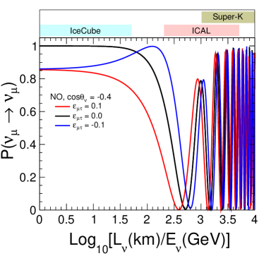
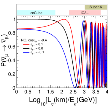
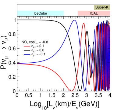
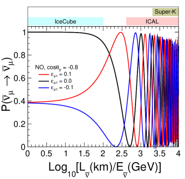
Figure 1: The survival probabilities of $\nu_{\mu}$ and $\bar{\nu}_{\mu}$ as functions of $\log_{10}(L_{\nu}/E_{\nu})$ in left and right panels, respectively. The black lines correspond to $\varepsilon_{\mu\tau}=0$ (standard interactions: SI), whereas red and blue lines are with $\varepsilon_{\mu\tau}=0.1$, and $-0.1$, respectively. The neutrino direction taken in upper (lower) panels is $\cos\theta_{\nu}=-0.4$ ($-0.8$). The horizontal bands shown here are the indicative $L_{\nu}/E_{\nu}$ ranges that these detectors are well-suited for. We consider normal mass ordering, and the benchmark oscillation parameters given in Table 2.

$\sin^{2}2\theta_{12}$	$\sin^{2}\theta_{23}$	$\sin^{2}2\theta_{13}$	$|\Delta m^{2}_{32}|$ (eV2)	$\Delta m^{2}_{21}$ (eV2)	$\delta_{\rm CP}$	Mass Ordering
0.855	0.5	0.0875	$2.46\times 10^{-3}$	$7.4\times 10^{-5}$	0	Normal (NO)

Table 2: The benchmark values of oscillation parameters that we use in the analysis. Normal mass ordering corresponds to $m_{1}<m_{2}<m_{3}$.

Figure 1 also indicates the sensitivity ranges for the atmospheric neutrino experiments Super-K, ICAL, and IceCube. Note that these ranges are different for $\cos\theta_{\nu}=-0.4$ and $-0.8$, which correspond to $L_{\nu}$ around 5100 km and 10200 km, respectively. While calculating these $L_{\nu}/E_{\nu}$ ranges, the energy ranges chosen are those for which the detectors perform very well: we use the $E_{\nu}$ range of 100 MeV – 5 GeV for Super-K Ashie:2005ik , 1–25 GeV for ICAL Kumar:2017sdq , and 100 GeV – 10 PeV for IceCube Aartsen:2013vja . Note that these ranges are only indicative. The following observations may be made from the figure.

• For $\log_{10}[L_{\nu}/E_{\nu}]$ in the range of [0 – 1.5], the survival probabilities of both $\nu_{\mu}$ and $\bar{\nu}_{\mu}$ are observed to be suppressed in the presence of non-zero $\varepsilon_{\mu\tau}$. This is because, although the oscillations due to neutrino mass-squared difference do not develop for such small value of $L_{\nu}/E_{\nu}$, i.e. $\Delta m^{2}_{32}L_{\nu}/E_{\nu}\ll 1$, the disappearance of $\nu_{\mu}$ is possible due to the $L_{\nu}\varepsilon_{\mu\tau}V_{\rm CC}$ term, which can be high for large baselines (for core passing neutrinos, $V_{\rm CC}$ is large). For example, log${}_{10}[L_{\nu}/E_{\nu}]=1$ may correspond to $L_{\nu}=5000$ km and $E_{\nu}=500$ GeV, so that $\Delta m^{2}_{32}L_{\nu}/E_{\nu}\approx 0.025$. However, for this baseline, the average density of the Earth is $\rho\approx 3.9$ g/cc, and hence for $\varepsilon_{\mu\tau}=0.1$, we have $L_{\nu}\varepsilon_{\mu\tau}V_{\rm CC}\approx 0.93$, which takes the oscillation probability away from unity. The effect of NSI at such small $L_{\nu}/E_{\nu}$ is energy-independent, and can be seen at detectors like IceCube Salvado:2016uqu due to its better performance at high energy. Note, however, that in the high energy limit, the $\nu_{\mu}$ survival probability depends only on the magnitude of $\varepsilon_{\mu\tau}$ (Eq. 9). As a result, it may be difficult for IceCube to determine sgn($\varepsilon_{\mu\tau}$), if indeed $|\varepsilon_{\mu\tau}|$ turns out to be nonzero.

• As we go to higher value of log${}_{10}[L_{\nu}/E_{\nu}]$ ($>2$), the term containing neutrino mass splitting becomes comparable to the $L\varepsilon_{\mu\tau}V_{\rm CC}$ term in Eq. 9, and the competition between these two terms leads to an energy dependence. When the oscillations due to the mass splitting are the dominating contribution, the change in oscillation wavelength due to non-zero $\varepsilon_{\mu\tau}$ results in a shift of the oscillation minima towards left or right side (lower or higher values of $L_{\nu}/E_{\nu}$, respectively), depending on the amplitude of $\varepsilon_{\mu\tau}$ and its sign. The direction of shift in the dip location depends on whether it is neutrino or antineutrino (since the sign of $V_{\rm CC}$ for them are opposite), and on the neutrino mass ordering. This effect on the shift in the dip location is discussed in next paragraph in detail. This region is relevant for Super-K, INO, and most of the long-baseline experiments.

We now discuss the modification of the oscillation dip due to non-zero $\varepsilon_{\mu\tau}$. First, using the approximate expression of $\nu_{\mu}$ survival probability from Eq. 9, we obtain the value of $L_{\nu}/E_{\nu}$ at the first oscillation minimum (or the dip):

$$\left.\frac{L_{\nu}}{E_{\nu}}\right|_{\rm dip}=\frac{2\pi}{|\Delta m^{2}_{32}+4\varepsilon_{\mu\tau}V_{\rm CC}E_{\nu}|}\,.$$ (10)

The above expression may be written by expressing $V_{\rm CC}$ in terms of the line-averaged matter density $\rho$ and taking care of units,

$$\left.\frac{L_{\nu}[{\rm km]}}{E_{\nu}[\rm GeV]}\right|_{\rm dip}=\frac{\pi}{\left|2.54\cdot\Delta m^{2}_{32}[{\rm eV^{2}}]\pm 7.7\times 10^{-4}\cdot\rho[{\rm g/cm^{3}}]\cdot Y_{e}\cdot\varepsilon_{\mu\tau}\cdot E_{\nu}[{\rm GeV}]\right|}\,.$$ (12)

Here, a positive sign in the denominator corresponds to neutrinos, whereas a negative sign is for antineutrinos. This approximation is useful for understanding the shift of dip position with non-zero $\varepsilon_{\mu\tau}$. Let us take the case of neutrino with normal ordering. With positive $\varepsilon_{\mu\tau}$, the denominator of Eq. 10 increases, thus the oscillation minimum appears at a lower value of $L_{\nu}/E_{\nu}$ than that for the SI. On the other hand, with negative $\varepsilon_{\mu\tau}$, the oscillation dip would occur at a higher value of $L_{\nu}/E_{\nu}$. These two features can be seen clearly in the left panels of Fig. 1. For antineutrinos and the same mass ordering, since the matter potential has the opposite sign, the shift of oscillation dip is in the opposite direction as compared to that for neutrinos, given the same $\varepsilon_{\mu\tau}$.

Expanding Eq. 12 to first order in $\varepsilon_{\mu\tau}$, one can write

$$\left.\frac{L_{\nu}[{\rm km}]}{E_{\nu}[{\rm GeV}]}\right|_{\rm dip}=\frac{\pi}{\left|2.54\times\Delta m^{2}_{32}[{\rm eV}^{2}]\right|}\mp\frac{\pi\times 1.19\times 10^{-4}\cdot\rho[{\rm g/cm^{3}}]\cdot Y_{e}\cdot E_{\nu}[{\rm GeV}]}{\beta\,(\Delta m^{2}_{32})^{2}[{\rm eV}^{4}]}\cdot\varepsilon_{\mu\tau}\,,$$ (13)

where $\beta\equiv{\rm sgn}(\Delta m^{2}_{32})$, as defined earlier. Here, the negative sign corresponds to neutrinos, whereas the positive sign is for antineutrino. This indicates that, for small values of $\varepsilon_{\mu\tau}$, the shift in the dip location will be linear in $\varepsilon_{\mu\tau}$, and will have opposite sign for neutrinos and antineutrinos, as well as for the two mass orderings. We have checked that for $E_{\nu}<25$ GeV and typical line-averaged density of the Earth, indeed $\varepsilon_{\mu\tau}<0.1$ is small enough for the above approximation to hold.

2.2 Effect of $\varepsilon_{\mu\tau}$ on the oscillation valley in the ($E_{\nu}$, $\cos\theta_{\nu}$) plane

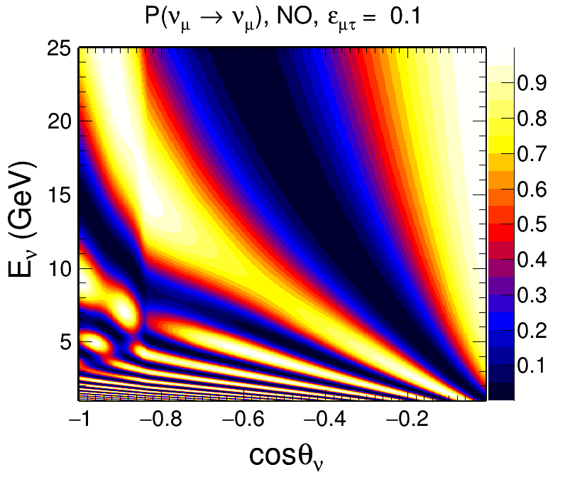
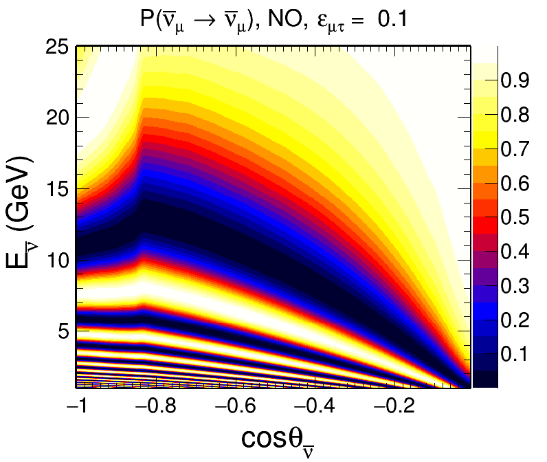
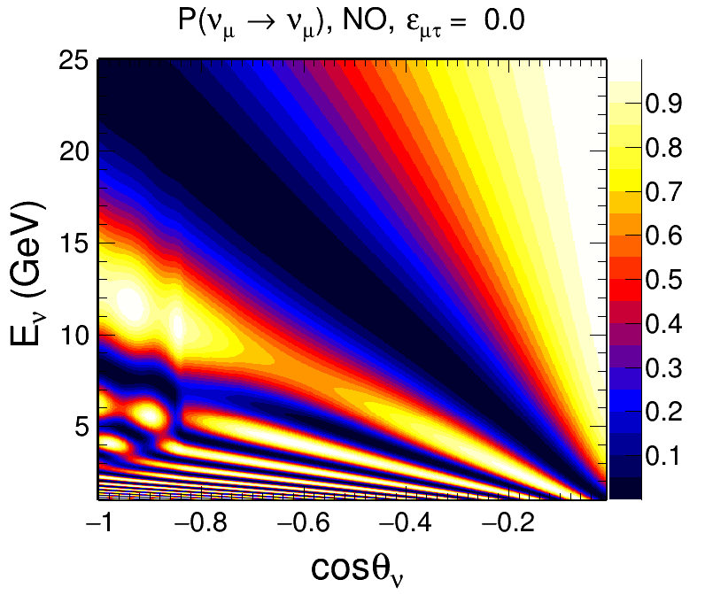
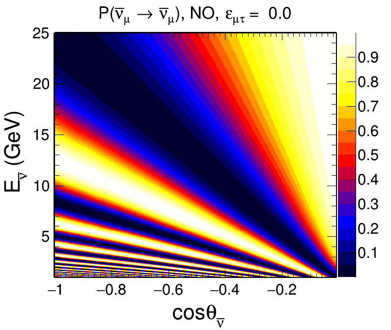
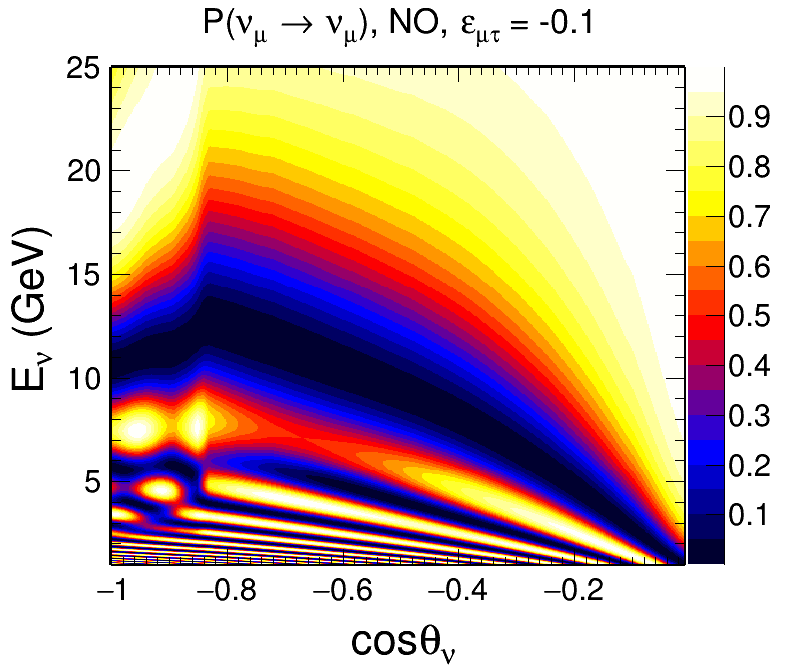
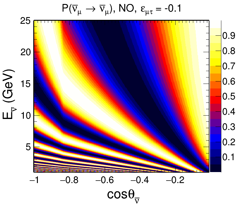
Figure 2: The oscillogram for the survival probabilities in ($E_{\nu},\cos\theta_{\nu}$) plane for neutrino and antineutrino in left and right panels, respectively, with normal mass ordering and the benchmark oscillation parameters from Table 2. The value of $\varepsilon_{\mu\tau}$ is taken as +0.1, 0 (SI), and -0.1 in top, middle and bottom panels, respectively.

In Fig. 2, we show the oscillograms of survival probabilities for $\nu_{\mu}$ and $\bar{\nu}_{\mu}$, in the plane of neutrino energy and cosine of neutrino zenith angle ($\cos\theta_{\nu}$), with NO as the neutrino mass ordering. We show only upward-going neutrinos ($\cos\theta_{\nu}<0$), since for downward-going neutrinos ($\cos\theta_{\nu}>0$), the baseline $L_{\nu}$ is very small and neutrino oscillations do not develop, making $P_{\mu\mu}\approx 1.0$. The differences observed among the upper, middle, and lower panels are due to different values of $\varepsilon_{\mu\tau}$. A major impact of NSI is observed on the feature corresponding to the first oscillation minima, seen in the figure as a broad blue/black diagonal band. We refer to this broad band as the oscillation valley Kumar:2020wgz . In the SI case, the oscillation valley appears like a triangle with straight edges, while in the presence of NSI, its edges seem to acquire a curvature. The sign of this curvature is opposite for neutrinos and antineutrinos, as can be seen by comparing the left and right plots of upper and lower panels of Fig. 2.

The modification in the oscillation valley due to NSI may be explained from the following relation between $E_{\nu}$ and $\cos\theta_{\nu}$ at the first oscillation minima. We rewrite Eq. 10 with $L_{\nu}\approx 2R|\cos\theta_{\nu}|$:

$$E_{\nu}|_{\rm valley}\approx\frac{|\Delta m^{2}_{32}|}{(\pi/|R\cos\theta_{\nu}|)\;-4\beta\,\varepsilon_{\mu\tau}V_{\rm CC}}\,.$$ (15)

Taking care of units and expressing $V_{\rm CC}$ in terms of line-averaged constant matter density $\rho$, the above expression may be written as

$$E_{\nu}[{\rm GeV}]|_{\rm valley}=\frac{|\Delta m^{2}_{32}[{\rm eV}^{2}]|}{(\pi/|5.08\cdot R[{\rm km}]\cdot\cos\theta_{\nu}|)\;\mp 3.02\times 10^{-4}\cdot\beta\cdot\varepsilon_{\mu\tau}\cdot Y_{e}\cdot\rho[{\rm g/cm^{3}}]}\,.$$ (16)

Here, the negative sign in the denominator corresponds to neutrinos, whereas the positive sign is for antineutrinos. Putting $\varepsilon_{\mu\tau}=0$ in Eq. 16 gives the condition of the first oscillation minima to be $E_{\nu}=|(5.08/\pi)\cdot\Delta m^{2}_{32}\cdot R[\rm km]\cdot\cos\theta_{\nu}|$, and this relation clearly shows that in the SI case, the minimum of the oscillation valley is a straight line in the ($E_{\nu}\,,\cos\theta_{\nu}$) plane.

Now in the normal mass ordering scenario, if $\varepsilon_{\mu\tau}>0$ in Eq. 16, then for neutrinos, $E_{\nu}$ increases for a given $\cos\theta_{\nu}$ as compared to the SI case. As a result, the oscillation valley (the broad blue/black band) bends towards higher values of energies in top left panel. On the other hand, for antineutrino, the oscillation valley tilts towards lower energies for $\varepsilon_{\mu\tau}>0$, as can be seen in the top right panel. For negative values of $\varepsilon_{\mu\tau}$, the oscillation valley bends in the opposite direction, for both neutrinos and antineutrinos, as shown in the bottom panels of Fig. 2. In the inverse mass ordering scenario, the bending of the oscillation valley will be in the direction opposite to that in the normal mass ordering scenario.

From Eqs. 13 and 16, the shift in the oscillation minima and the bending in the oscillation valley are in opposite directions for normal and inverted mass ordering. The effect of $\varepsilon_{\mu\tau}$, therefore, depends crucially on the mass ordering. In this paper, we present our analysis in the scenario where the mass ordering is known to be NO. The analysis for IO may be performed in an exactly analogous manner. Our results are presented with the exposure corresponding to 10 years of ICAL data-taking. It is expected that the mass ordering will be determined from the neutrino experiments (including ICAL) by this time.

3 Impact of NSI on the Event Distribution at ICAL

While the effect of NSI on the neutrino and antineutrino survival probabilities was discussed in the last section, it is important to confirm whether the features present at the probability level can survive in the observables at a detector, and if they can be reconstructed. Here is where the response of the detector plays a crucial role. Neutrinos cannot be directly detected in an experiment, however the charged leptons produced from their charged-current interactions in the detector contains information about their energy, direction, and flavor, which can be recovered depending on the nature of the detector.

The upcoming ICAL detector at the India-based Neutrino Observatory (INO) will be composed of 151 layers of magnetized iron plates; the 50 kt iron acting as the target, and around 30,000 glass resistive plate chambers as detection elements. The magnetic field of strength 1.5 Tesla and the time resolution of less than 1 ns Dash:2014ifa ; Bhatt:2016rek ; Gaur:2017uaf will enable ICAL to distinguish $\mu^{-}$ from $\mu^{+}$ events in the multi-GeV energy range. In this study, we generate the charged-current interactions of $\nu_{\mu}$ and $\bar{\nu}_{\mu}$, similar to Ref. Kumar:2020wgz , using neutrino and antineutrino fluxes calculated at the Theni site by Honda et.al. Athar:2012it ; PhysRevD.92.023004 and the neutrino event generator NUANCE Casper:2002sd . The reconstructed energy ($E_{\mu}^{\rm rec}$) and zenith angle ($\theta_{\mu}^{\rm rec}$) of muons produced in neutrino and antineutrino interactions will be used in the analysis. The detector properties of ICAL for muons as obtained in Ref.Chatterjee:2014vta using the ICAL-GEANT4 simulation package, are incorporated. With around 1 km rock coverage (3800 meter water equivalent), the downward-going cosmic muon background would get reduced by $\sim 10^{6}$ Dash:2015blu , most of which will be further vetoed by employing the fiducial volume cut. We do not consider the muon events induced by tau decay in the detector since the number of such events is small ($\sim 2\%$ of total upward-going muons from $\nu_{\mu}$ interactions in the energy range of interest Pal:2014tre ), and these are mostly at lower energies and below the energy threshold of ICAL which is 1 GeV.

The quantity $L_{\mu}^{\rm rec}$ associated with the reconstructed muon direction $\cos\theta_{\mu}^{\rm rec}$ is defined (similar to Eq. 14) as

$$L_{\mu}^{\rm rec}\equiv\sqrt{(R+h)^{2}-(R-d)^{2}\sin^{2}\theta_{\mu}^{\rm rec}}\,-\,(R-d)\cos\theta_{\mu}^{\rm rec}\,.$$ (17)

Note that $L_{\mu}^{\rm rec}$ is simply a proxy observable, and there is no need to associate it directly with the distance traveled by the incoming neutrino.

3.1 The $L_{\mu}^{\text{rec}}/E_{\mu}^{\text{rec}}$ distributions

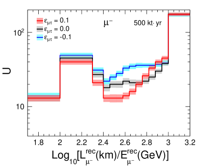
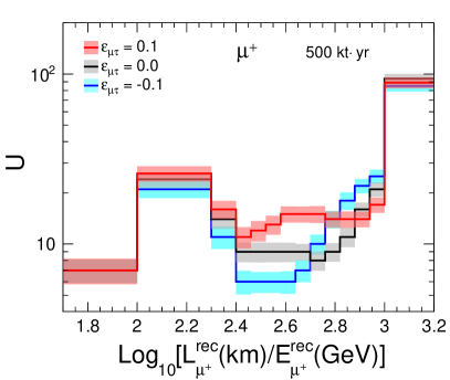
Figure 3: The $\log_{10}[L_{\mu}^{\text{rec}}/E_{\mu}^{\text{rec}}]$ distributions of $\mu^{-}$ and $\mu^{+}$ events in left and right panels, respectively, expected in 10 years at ICAL. The black lines correspond to SI ($\varepsilon_{\mu\tau}=0$), whereas red and blue lines are for $\varepsilon_{\mu\tau}=0.1$ and -0.1, respectively. The statistical uncertainties shown by shaded boxes are the root-mean square (rms) fluctuations of 100 independent 10-year data sets. The solid lines show the mean of these 100 distributions. We consider normal mass ordering, and the benchmark oscillation parameters given in Table 2.

Observable	Range	Bin width	Number of bins
$\log_{10}\left[\frac{L_{\mu}^{\rm rec}(\text{km})}{E_{\mu}^{\rm rec}(\text{GeV})}\right]$	[0, 1]	0.2	5	}77mm[34]
	[1, 1.6]	0.06	10
	[1.6, 1.7]	0.1	1
	[1.7, 2.3]	0.3	2
	[2.3, 2.4]	0.1	1
	[2.4, 3.0]	0.06	10
	[3, 4]	0.2	5

Table 3: The binning scheme of $\log_{10}[L_{\mu}^{\rm rec}/E_{\mu}^{\rm rec}]$ for $\mu^{-}$ and $\mu^{+}$ events.

Fig. 3 presents the $\log_{10}[L_{\mu}^{\text{rec}}/E_{\mu}^{\text{rec}}]$ distribution of the upward-going $\mu^{-}$ and $\mu^{+}$ events (U, $\cos\theta_{\mu}^{\rm rec}<0$) with SI ($\varepsilon_{\mu\tau}=0$) and with SI + NSI ($\varepsilon_{\mu\tau}=\pm 0.1$) expected with 10-year exposure at ICAL. We include the statistical fluctuation in the number of events by simulating 100 independent data sets, and calculating the mean and root-mean-square deviation for each bin. For $\log_{10}[L_{\mu}^{\text{rec}}/E_{\mu}^{\text{rec}}]$, we use the same binning scheme as used in Ref. Kumar:2020wgz , which is shown in Table 3. We have a total of 34 non-uniform bins of $\log_{10}[L_{\mu}^{\text{rec}}/E_{\mu}^{\text{rec}}]$ in the range 0–4. The downward-going events (D, $\cos\theta_{\mu}^{\text{rec}}>0$) are not affected significantly by oscillations or by additional NSI interactions. The $\log_{10}[L_{\mu}^{\text{rec}}/E_{\mu}^{\text{rec}}]$ distribution of downward-going $\mu^{-}$ and $\mu^{+}$ events is identical to the one shown in the upper panel of Fig. [4] in Ref. Kumar:2020wgz , and we do not repeat it here.

Fig. 3 clearly shows that the $\log_{10}[L_{\mu}^{\text{rec}}/E_{\mu}^{\text{rec}}]$ range of 2.4–3.0 would be important for NSI studies, since non-zero $\varepsilon_{\mu\tau}$ has the largest effect in this range. With positive $\varepsilon_{\mu\tau}$, the number of $\mu^{-}$ events is lower as compared to that of SI case, whereas the number of $\mu^{+}$ events is higher. If $\varepsilon_{\mu\tau}$ is negative, then the modifications of the number of $\mu^{-}$ and $\mu^{+}$ events are the other way around. As a consequence, if a detector is not able to distinguish between the $\mu^{-}$ and $\mu^{+}$ events, the difference between SI and NSI would get diluted substantially. The charge identification capability of the magnetized ICAL detector would be crucial in exploiting this observation.

3.2 Distributions in the ($E_{\mu}^{\rm rec}$, $\cos\theta_{\mu}^{\rm rec}$) plane

In order to study the effect of NSI on the distribution of events in the ($E_{\mu}^{\rm rec}$, $\cos\theta_{\mu}^{\rm rec}$) plane, we bin the data in reconstructed observables, $E_{\mu}^{\rm rec}$ and $\cos\theta_{\mu}^{\rm rec}$. We have a total of 16 non-uniform $E_{\mu}^{\rm rec}$ bins in the range 1 – 25 GeV, and the whole range of $-1\leq\cos\theta_{\mu}^{\rm rec}\leq 1$ is divided into 20 uniform bins. The reconstructed $E_{\mu}^{\rm rec}$ and $\cos\theta_{\mu}^{\rm rec}$ are binned with the same binning scheme as used in Kumar:2020wgz , and is shown in Table 4. For demonstrating event distributions, we scale the 1000-year MC sample to an exposure of 10 years, and the difference in the number of events with SI + NSI ($|\varepsilon_{\mu\tau}|=0.1$) and the number of events with SI, for $\mu^{-}$ and $\mu^{+}$ events are shown in Fig. 4.

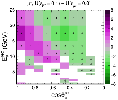
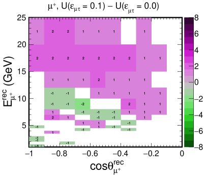
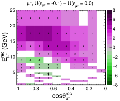
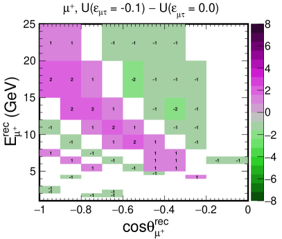
Figure 4: The $(E_{\mu}^{\text{rec}},\,\cos\theta_{\mu}^{\text{rec}})$ distributions of difference of events between including non-zero NSI and only SI ($\varepsilon_{\mu\tau}=0$) expected with 500 kt$\cdot$yr of ICAL. Left and right panels are for $\mu^{-}$ and $\mu^{+}$ events, respectively, whereas upper and lower panels correspond to $\varepsilon_{\mu\tau}=0.1$ and $-0.1$, respectively. We consider normal mass ordering, and the benchmark oscillation parameters given in Table 2.

Observable	Range	Bin width	Number of bins
$E_{\mu}^{\rm rec}$	[1, 5]	0.5	8	}57mm[16]
	[5, 8]	1	3
(GeV)	[8, 12]	2	2
	[12, 15]	3	1
	[15, 25]	5	2
$\cos\theta_{\mu}^{\rm rec}$	[-1.0, 1.0]	0.1	20

Table 4: The binning scheme adopted for $E_{\mu}^{\rm rec}$ and $\cos\theta_{\mu}^{\rm rec}$ of $\mu^{-}$ and $\mu^{+}$ events.

From this figure, we can make the following observations.

• The events in the bins with $E_{\mu}^{\text{rec}}>5$ GeV and $\cos\theta_{\mu}^{\text{rec}}<-0.2$ are particularly useful for NSI searches at ICAL. This is true for both $\mu^{-}$ and $\mu^{+}$ events.

• There is almost no difference in the number of events between SI+NSI and SI at $E_{\mu}^{\text{rec}}<5$ GeV. The events with reconstructed muon energy less than 5 GeV do not seem to be sensitive to NSI due to small NSI-induced matter effects: $L_{\nu}\varepsilon_{\mu\tau}V_{\rm CC}\lesssim\Delta m^{2}/(2E_{\nu})$ at small energies.

• As we go to higher energies, the mass-squared difference-induced neutrino oscillations die down, while the NSI-induced matter effect term $L_{\nu}\varepsilon_{\mu\tau}V_{\rm CC}$ increases. Therefore, large effects of NSI are observed at high energies.

• The effect of NSI is also larger at higher baselines, since in this case, neutrinos pass through inner and outer cores that have very high matter densities (around 13 g/cm³ and 11 g/cm³, respectively), and hence higher values of $L_{\nu}\varepsilon_{\mu\tau}V_{\rm CC}$.

• In many of the $(E_{\mu}^{\text{rec}},\,\cos\theta_{\mu}^{\text{rec}})$ bins, NSI gives rise to an excess in $\mu^{-}$ events and a deficit in $\mu^{+}$ events, or vice versa. If $\mu^{-}$ and $\mu^{+}$ events are not separated, this would lead to a dilution of information. Therefore, muon charge information is a crucial ingredient in the search for NSI. We have also seen this feature in the $\log_{10}[L_{\mu}^{\text{rec}}/E_{\mu}^{\text{rec}}]$ distributions of $\mu^{-}$ and $\mu^{+}$ events in Sec. 3.1.

4 Identifying NSI through the Shift in Oscillation Dip Location

To study the effect of NSI in oscillation dip, we focus on the ratio of upward-going (U) and downward-going (D) muon events as the observable to be studied. The up/down event ratio U/D is defined for $\cos\theta_{\mu}^{\rm rec}<0$, as Kumar:2020wgz

$${\text{U/D}}(E_{\mu}^{\rm rec},\,\cos\theta_{\mu}^{\rm rec})\equiv\frac{N(E_{\mu}^{\rm rec},\,-|\cos\theta_{\mu}^{\rm rec}|)}{N(E_{\mu}^{\rm rec},\,|\cos\theta_{\mu}^{\rm rec}|)}\,,$$ (18)

where the numerator corresponds to the number of upward-going events and the denominator is the number of downward-going events, with energy $E_{\mu}^{\rm rec}$ and direction $|\cos\theta_{\mu}^{\rm rec}|$. We associate the U/D ratio with $\cos\theta_{\mu}^{\rm rec}<0$ as well as the corresponding $L_{\mu}^{\rm rec}$ of upward-going events. This ratio is expected to serve as the proxy for the survival probabilities of $\nu_{\mu}$ and $\bar{\nu}_{\mu}$ at ICAL, since around 98$\%$ muon events at ICAL arise from the $\nu_{\mu}\rightarrow\nu_{\mu}$ oscillation channel Kumar:2020wgz .

One advantage of the use of the U/D ratio would be to nullify the effects of systematic uncertainties like flux normalization, cross sections, overall detection efficiency, and energy dependent tilt error, as can be seen later. Note that the up-down symmetry of the detector geometry and detector response play an important role in this.

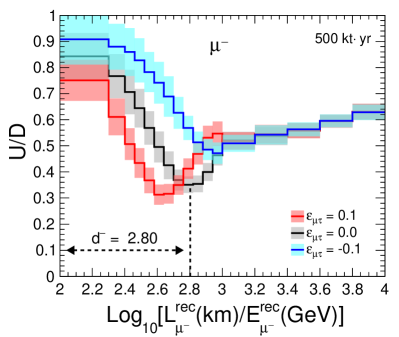
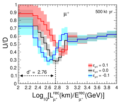
Figure 5: The $\log_{10}(L_{\mu}^{\text{rec}}/E_{\mu}^{\text{rec}})$ distributions of ratio of upward-going and downward-going $\mu^{-}$ (left panel) and $\mu^{+}$ (right panel) events using 10-year data of ICAL. The black lines correspond to SI ($\varepsilon_{\mu\tau}=0$), whereas red and blue lines are for $\varepsilon_{\mu\tau}=0.1$ and -0.1, respectively. The statistical fluctuations shown by shaded boxes are the root-mean-square deviation of 100 independent distributions of U/D ratio, each for 10 years, whereas the mean of these distributions are shown by solid lines. We consider normal mass ordering, and the benchmark oscillation parameters given in Table 2.

Fig. 5 presents the $L_{\mu}^{\text{rec}}/E_{\mu}^{\text{rec}}$ distributions of U/D with $\varepsilon_{\mu\tau}=0$ (SI) and $\pm 0.1$, for an exposure of 10 years at ICAL. The mass ordering is taken as NO. The statistical fluctuations shown in the figure are the root-mean-square deviation obtained from the simulations of 100 independent sets of 10 years data. Around $\log_{10}[L_{\mu}^{\text{rec}}/E_{\mu}^{\text{rec}}]\sim 2.4-2.6$, we see a significant modification in the U/D ratio due to the presence of non-zero $\varepsilon_{\mu\tau}$ ($\pm 0.1$), particularly in the location of the oscillation dip. The dip shifts towards left or right (i.e. to lower or higher values of $L_{\mu}^{\rm rec}/E_{\mu}^{\rm rec}$, respectively) from that of the SI case with non-zero $\varepsilon_{\mu\tau}$. This shift for $\mu^{-}$ and $\mu^{+}$ events is observed to be in opposite directions, as is expected from the discussions in Sec. 2.1. For example, for $\varepsilon_{\mu\tau}>0$, the location of oscillation dip in $\mu^{-}$ events gets shifted towards smaller $L_{\mu}^{\text{rec}}/E_{\mu}^{\text{rec}}$ values. On other hand, in $\mu^{+}$ events, the oscillation dip shifts to higher values of $L_{\mu}^{\text{rec}}/E_{\mu}^{\text{rec}}$. For $\varepsilon_{\mu\tau}<0$, this shift is in the opposite directions. Moreover, as the oscillation dip shifts towards the higher value of $L_{\mu}^{\text{rec}}/E_{\mu}^{\text{rec}}$, the dip becomes shallower due to the effect of rapid oscillation at high $L_{\nu}/E_{\nu}$. This effect is visible in both, $\mu^{-}$ and $\mu^{+}$. It can be easily argued that the modification in oscillation dips of $\mu^{-}$ and $\mu^{+}$ due to non-zero $\varepsilon_{\mu\tau}$ is the reflection of how the survival probabilities of neutrino and antineutrino change in the presence of non-zero $\varepsilon_{\mu\tau}$, as expected from Eq. 10 in Sec. 2.1.

Note that for a neutrino detector that is blind to the charge of muons, the dip itself would get diluted since different average inelasticities of neutrino and antineutrino events at these energies would lead to slightly different dip locations in $\mu^{-}$ and $\mu^{+}$ distributions. Moreover, the shift of oscillation dip towards opposite directions in $\mu^{-}$ and $\mu^{+}$ events due to non-zero $\varepsilon_{\mu\tau}$ would further contribute to the dilution of NSI effects on the dip location. On the other hand, a detector like ICAL that has the charge identification capability, not only provides independent undiluted measurements of dip locations in $\mu^{-}$ and $\mu^{+}$ events, but also provides a unique novel observable that can cleanly calibrate against the value of $\varepsilon_{\mu\tau}$, as we shall see in the next section.

4.1 A novel variable $\Delta d$ for determining $\varepsilon_{\mu\tau}$

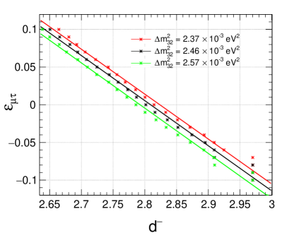
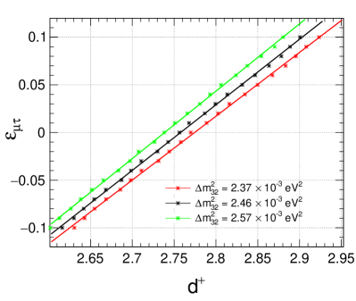
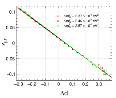
Figure 6: Upper panels: The calibration of $\varepsilon_{\mu\tau}$ with the dip location in U/D ratio of $\mu^{-}$ (left panel) and $\mu^{+}$ (right panel) events separately. Lower panel: The calibration of $\varepsilon_{\mu\tau}$ with difference in dip location of $\mu^{-}$ and $\mu^{+}$. Note that for $-0.1<\varepsilon_{\mu\tau}<-0.07$, the dip location is simply the center of the $\log_{10}[L_{\mu}^{\text{rec}}/E_{\mu}^{\text{rec}}]$ bin with minimum U/D ratio since the fitting is not stable for these values. We consider normal mass ordering, and the benchmark oscillation parameters given in Table 2.

Since the oscillation dip locations in the U/D distributions of both, $\mu^{-}$ and $\mu^{+}$ events, shift to lower / higher values of $L_{\mu}^{\text{rec}}/E_{\mu}^{\text{rec}}$ depending on the value of $\varepsilon_{\mu\tau}$, the dip location in either of these distributions may be used to estimate $\varepsilon_{\mu\tau}$, independently. We have already developed a dip-identification algorithm Kumar:2020wgz , where the dip location is not simply the lowest value of U/D ratio, but takes into account information from the surrounding bins that have a U/D ratio below a threshold value. The algorithm essentially identifies the cluster of contiguous bins that have a U/D ratio lower than any surrounding bins, and fits these bins with a quadratic function whose minimum corresponds to the dip. The value of $\log_{10}[L_{\mu}^{\text{rec}}/E_{\mu}^{\text{rec}}]$ corresponding to this minimum is termed as the dip location. We denote the dip location for $\mu^{-}$ and $\mu^{+}$ events as $d^{-}$ and $d^{+}$, respectively.

We obtain the calibration of $\varepsilon_{\mu\tau}$ with the dip locations for $\mu^{-}$ and $\mu^{+}$ events separately, using 1000-year MC data. In the top panels of Fig. 6, we present the calibration curves of $\varepsilon_{\mu\tau}$ with $d^{-}$ (left panel) and $d^{+}$ (right panel), for three different values of $\Delta m^{2}_{32}$. The straight line nature of the calibration curves can be understood qualitatively using Eq. 10. For a majority of events ($E_{\mu}^{\text{rec}}<25$ GeV), the $\varepsilon_{\mu\tau}V_{\rm CC}E_{\nu}$ term is much smaller than $\Delta m^{2}_{32}$ term, and therefore the linear expansion as shown in Eq. 13 is valid.

In Eq. 13, the dominating $\Delta m^{2}_{32}$ dependence of the dip location is through the first term. We can get rid of this dependence by introducing a new variable

$$\Delta d=d^{-}-d^{+}\,,$$ (19)

which is expected to be proportional to $\varepsilon_{\mu\tau}$, and can be used to calibrate for $\varepsilon_{\mu\tau}$. As may be seen in the bottom panel of Fig. 6, this indeed removes the dominant $\Delta m^{2}_{32}$-dependence in the calibration of $\varepsilon_{\mu\tau}$. Note that some $\Delta m^{2}_{32}$-dependence still survives, which may be seen in the slightly different slopes of the calibration curves for different $\Delta m^{2}_{32}$ values. However, this dependence is clearly negligible, as it appears in Eq. 13 as a multiplicative correction to $\varepsilon_{\mu\tau}$. We have thus obtained a calibration for $\varepsilon_{\mu\tau}$ that is almost independent of $\Delta m^{2}_{32}$.

Note that $\varepsilon_{\mu\tau}=0$ does not imply $\Delta d=0$, since different matter effects and different inelasticities in neutrino and antineutrino channels cause the dips to arise at slightly different $\log_{10}[L_{\mu}^{\text{rec}}/E_{\mu}^{\text{rec}}]$ values in these two channels even in the absence of NSI.

4.2 Constraints on $\varepsilon_{\mu\tau}$ from the measurement of $\Delta d$

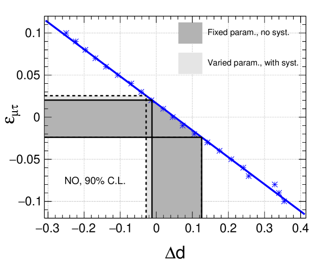
Figure 7: The blue stars and the blue solid line indicate the calibration curve of $\varepsilon_{\mu\tau}$ against $\Delta d$, obtained using 1000-year MC data with normal mass ordering. The gray bands show the expected 90% C.L. limits on $\Delta d$ (vertical bands), and hence on $\varepsilon_{\mu\tau}$ (horizontal bands), with 500 kt$\cdot$yr of ICAL exposure, when the actual value of $\varepsilon_{\mu\tau}=0$. The light (dark) gray bands show the limits when the errors on oscillation parameters, and the impact of systematic uncertainties are included (excluded), as discussed in Sec. 4.2. For fixed-parameter case, we use the benchmark oscillation parameters given in Table 2.

We saw in the last section that one can infer the value of $\varepsilon_{\mu\tau}$ in the observed data from the calibration curve between $\Delta d$ and $\varepsilon_{\mu\tau}$, independent of the actual value of $\Delta m^{2}_{32}$. We obtain the calibration curve using the 1000-year MC-simulated sample, and show it with the solid blue line in Fig. 7.

For estimating the expected constraints on $\varepsilon_{\mu\tau}$, we simulate 100 independent sets of data, each for 10-year exposure of ICAL with the benchmark oscillation parameters as given in Table 2, and $\varepsilon_{\mu\tau}=0$. In Fig. 7, the range indicated along the x-axis by dark gray band is the expected 90% C.L. range of the measured value of $\Delta d$, while the range indicated along the y-axis by the dark gray band is the expected 90% C.L. limit on $\varepsilon_{\mu\tau}$. From the figure, we find that one can expect to constrain $\varepsilon_{\mu\tau}$ to $-0.024<\varepsilon_{\mu\tau}<0.020$ at 90% C.L. with 10 years of data.

Since the calibration was found to be almost independent of the actual value of $\Delta m^{2}_{32}$, we expect that even if the actual value of $\Delta m^{2}_{32}$ were not exactly known, the results will not change. We have confirmed this by generating 100 independent sets of 10-year exposure, where the $\Delta m^{2}_{32}$ values used as inputs follow a Gaussian distribution $\Delta m^{2}_{32}=(2.46\pm 0.03)\times 10^{-3}$ eV², in accordance to the range allowed by the global fit deSalas:2020pgw ; Esteban:2020cvm ; Capozzi:2017ipn of available neutrino data.

We also checked the impact of uncertainties in the values of the other oscillation parameters. We first simulated 100 statistically independent unoscillated data sets. Then for each of these data sets, we take 20 random choices of oscillation parameters, according to the Gaussian distributions

$$\Delta m^{2}_{21}=(7.4\pm 0.2)\times 10^{-5}\mbox{ eV}^{2}~{},\Delta m^{2}_{32}=(2.46\pm 0.03)\times 10^{-5}\mbox{ eV}^{2}~{},$$ (20)

$$\sin^{2}2\theta_{12}=0.855\pm 0.020~{},~{}\sin^{2}2\theta_{13}=0.0875\pm 0.0026~{},~{}\sin^{2}\theta_{23}=0.50\pm 0.03~{},$$ (21)

guided by the present global fit NUFIT . We keep $\delta_{\rm CP}=0$, since its effect on $\nu_{\mu}$ survival probability is known to be highly suppressed in the multi-GeV energy range Kopp:2007ne . This procedure effectively enables us to consider the variation of our results over 2000 different combinations of oscillation parameters, to take into account the effect of their uncertainties.

We do not observe any significant dilution of results due to the variation over oscillation parameters. This is expected, since (i) solar oscillation parameters $\Delta m^{2}_{21}$ and $\theta_{12}$ do not contribute significantly to the $\nu_{\mu}$ survival probability in the multi-GeV range, (ii) the reactor mixing angle $\theta_{13}$ is already measured to a high precision, (iii) the mixing angle $\theta_{23}$ does not affect the location of the oscillation minimum at the probability level, and (iv) our procedure of using $\Delta d$ (see Eq. 19) to determine $\varepsilon_{\mu\tau}$ minimizes the impact of $\Delta m^{2}_{32}$ uncertainty, as shown in Sec. 4.1.

In addition, we take into account the five major systematic uncertainties in the neutrino fluxes and cross sections that are used in the standard ICAL analyses Kumar:2017sdq . These five uncertainties are (i) 20% in overall flux normalization, (ii) 10% in cross sections, (iii) 5% in the energy dependence, (iv) 5% in the zenith angle dependence, and (v) 5% in overall systematics. For each of the 2000 simulated data sets, we modify the number of events in each $(E_{\mu}^{\rm rec},\cos\theta_{\mu}^{\rm rec})$ bin as

$$N=N^{(0)}(1+\delta_{1})(1+\delta_{2})(E_{\mu}^{\rm rec}/E_{0})^{\delta_{3}}(1+\delta_{4}\cos\theta_{\mu}^{\rm rec})(1+\delta_{5})~{},$$ (22)

where $N^{(0)}$ is the theoretically predicted number of events, and $E_{0}=2$ GeV. Here, $(\delta_{1},\delta_{2},\delta_{3},\delta_{4},\delta_{5})$ is an ordered set of random numbers, generated separately for each simulated data set, with the Gaussian distributions centered around zero and the $1\sigma$ widths given by $(20\%,10\%,5\%,5\%,5\%)$. The normalization uncertainties and energy tilt uncertainty are expected to be canceled in the U/D ratio, while the zenith angle distribution uncertainty affects the upward-going and downward-going events differently, and hence would be expected to affect the U/D ratio. We explicitly check this and indeed find this to be true.

When the oscillation parameter uncertainties and all the five systematic uncertainties mentioned above are included, it is found that the method based on the shift in the dip locations may constrain $\varepsilon_{\mu\tau}$ to $-0.025<\varepsilon_{\mu\tau}<0.024$ at 90% C.L.. The results denoting the effects of these uncertainties have been shown in Fig. 7.

5 A New Method for Determining $\Delta m^{2}_{32}$ in the Absence of NSI

The reconstruction of the oscillation valley using the distributions of the upward-going and downward-going muons in $(E^{\rm rec}_{\mu},\,\cos\theta_{\mu}^{\rm rec})$ plane is discussed in detail in Ref. Kumar:2020wgz . It has been shown that the alignment of the valley can provide a measurement of $\Delta m^{2}_{32}$. In this paper, we use an alternative procedure for getting the alignment of the oscillation valley, which is more robust and more well-motivated as compared to what was used in Ref. Kumar:2020wgz , and determine the expected precision that the ICAL detector can achieve on the atmospheric oscillation parameter $\Delta m^{2}_{32}$, using this method.

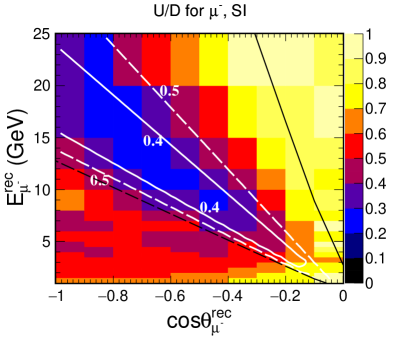
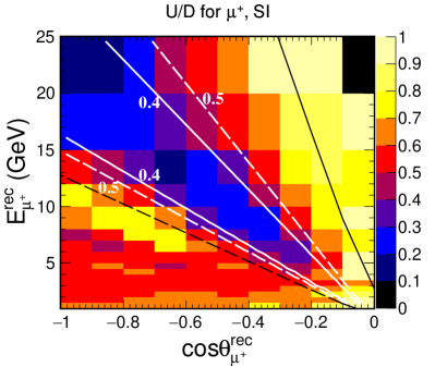
Figure 8: The distributions of U/D ratios in ($E_{\mu}^{\rm rec}$, $\cos\theta_{\mu}^{\rm rec}$) plane, for $\mu^{-}$ and $\mu^{+}$ events, in left and right panels, respectively. This is the average of 100 independent simulated data sets, each for 10-year exposure at ICAL, with $\varepsilon_{\mu\tau}=0$. The white solid and dashed lines correspond to the contours with fitted U/D ratio equal to 0.4 and 0.5, respectively, obtained after the fitting of oscillation valley with the function $F_{0}$ as given in Eq. 23. The black solid and dashed lines correspond to $\log_{10}[L_{\mu}^{\text{rec}}/E_{\mu}^{\text{rec}}]=$ 2.2 and 3.0, respectively. We consider normal mass ordering, and the benchmark oscillation parameters given in Table 2.

Fig. 8 shows the distributions of the ratio of upward-going and downward going events at ICAL in the $(E_{\mu}^{\rm rec}$, $\cos\theta_{\mu}^{\rm rec})$ plane for 10 years of ICAL data. The left and right panels show the U/D ratios for $\mu^{-}$ and $\mu^{+}$ events, respectively. For the sake of demonstration (in order to reduce the statistical fluctuations in the figure and emphasize the physics), we show the binwise average of 100 independent data sets, each with 10-year exposure of ICAL. The blue bands in Fig. 8 correspond to the reconstructed oscillation valley. Note that a good reconstruction of the oscillation valley would be an evidence for the fidelity of the ICAL detector.

To get the alignment of the oscillation valley, we fit the U/D distribution for $\mu^{-}$ or $\mu^{+}$ independently with a functional form

$$F_{0}(E_{\mu}^{\rm rec},\cos\theta_{\mu}^{\rm rec})=Z_{0}+N_{0}\cos^{2}\left(m_{0}\frac{\cos\theta_{\mu}^{\rm rec}}{E_{\mu}^{\rm rec}}\right),$$ (23)

where $Z_{0}$, $N_{0}$, and $m_{0}$ are the independent parameters to be determined from the fitting of U/D distributions. The parameter $Z_{0}$ quantifies the minimum depth of the fitted U/D ratio, $N_{0}$ is the normalization constant, whereas $m_{0}$ is the slope of the oscillation valley. Since more than $95\%$ of the events at ICAL are contributed from the $\nu_{\mu}\to\nu_{\mu}$ and $\bar{\nu}_{\mu}\to\bar{\nu}_{\mu}$ survival probabilities, we expect that the function $F_{0}$, that resembles Eq. 9, would be suitable for fitting the oscillation valley in the $(E_{\mu}^{\rm rec}$, $\cos\theta_{\mu}^{\rm rec})$ plane. Here, the slope $m_{0}$ can be used directly to calibrate $\Delta m^{2}_{32}$. The parameters $N_{0}$ and $Z_{0}$ also contain information about the atmospheric mixing parameters, however, they cannot be connected easily to the determinations of these parameters.

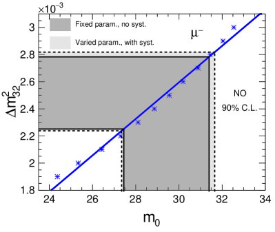
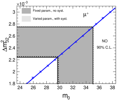
Figure 9: The blue stars and the blue lines indicate the calibration curves of $\Delta m^{2}_{32}$ against $m_{0}$, obtained using 1000-year MC data with normal mass ordering. The gray bands represent the 90% C.L. allowed ranges of $m_{0}$ (vertical bands), and hence of $\Delta m^{2}_{32}$ (horizontal bands), with a given input value of $\Delta m^{2}_{32}$ = 2.46$\times 10^{-3}$ eV², for an exposure of 10 years at ICAL. The results for $\mu^{-}$ and $\mu^{+}$ events are shown separately, in the left and right panels, respectively. The light (dark) gray bands show the ranges when the errors on other oscillation parameters and the impact of systematic uncertainties are included (excluded), as discussed in Sec. 4.2. For fixed-parameter case, we use the benchmark oscillation parameters given in Table 2.

Figure 8 also shows the contour lines for the fitted U/D ratio of 0.4 and 0.5. The contour lines for $\mu^{+}$ are seen to reproduce the data better than those for $\mu^{-}$. The reason behind this is the matter effects, which appear in $\mu^{-}$ data since the mass ordering is assumed to be NO here. Note that the fitting function $F_{0}$ is designed for only the vacuum oscillation, and we focus only on the region where vacuum oscillation is expected to dominate. In order to be safe from matter effects, we remove the events with $\log_{10}[L_{\mu}^{\text{rec}}/E_{\mu}^{\text{rec}}]>3.0$, where the matter effects are significant. We also discard the events with $\log_{10}[L_{\mu}^{\text{rec}}/E_{\mu}^{\text{rec}}]<2.2$, since these would have barely oscillated. The latter cut also gets rid of most of the events near horizon, where the distance traveled by the neutrinos has large errors. In order to minimize the data from the bins with clearly large fluctuations, we use another cut on the maximum value of the U/D ratio. This cut is taken to be U/D $<0.9$ for both $\mu^{-}$ and $\mu^{+}$ events.

We calibrate for $\Delta m^{2}_{32}$ by fitting the U/D ratio of 1000-year MC data with input $\Delta m^{2}_{32}$ values in the range $(1.9-3.0)\times 10^{-3}$ eV², and obtaining the corresponding value of $m_{0}$. The statistical fluctuations are estimated by simulating 100 independent data sets of 10 years for a given input value of $\Delta m^{2}_{32}$ $=2.46\times 10^{-3}$ eV², and fitting for the U/D ratio independently with Eq. 23. The 100 values of $m_{0}$ thus obtained provide the expected uncertainties on $\Delta m^{2}_{32}$. In Fig. 9, the gray bands show the $90\%$ C.L. ranges expected to be inferred by this method in 10 years. The figure also shows the (small) deterioration in the $90\%$ C.L. range of $\Delta m^{2}_{32}$ due to the incorporation of the present uncertainties in the oscillation parameters, and all the five systematic errors, as discussed in Sec. 4.2. With systematic uncertainties and error in other oscillation parameters, we get the expected $90\%$ C.L. allowed range for $\Delta m^{2}_{32}$ from $\mu^{-}$ events as (2.24 – 2.82)$\times 10^{-3}$ eV² and from $\mu^{+}$ events as (2.25 – 2.75)$\times 10^{-3}$ eV².

An advantage of the method proposed in this section over the original proposal in Kumar:2020wgz is that this is a one-step fitting procedure as opposed to the two-step fitting procedure therein. Note that the results obtained by this method are also slightly better than the ones obtained in Kumar:2020wgz , as the shape of the valley is explicitly fitted to. Moreover, we can extend this method to measure other characteristics of the oscillation valley, such as identifying the signature of NSI, which we shall discuss in the next section.

6 Identifying NSI through Oscillation Valley

So far, we have discussed the characteristics of the oscillation valley in the absence of NSI ($\varepsilon_{\mu\tau}=0$), and the measurement of $\Delta m^{2}_{32}$ in this scenario. In this section, we explore the features of the oscillation valley in the presence of NSI (non-zero $\varepsilon_{\mu\tau}$). We have already observed in Sec. 2.2 that in the presence of non-zero $\varepsilon_{\mu\tau}$, the oscillation valley in the oscillogram has a curved shape that depends on the extent of $\varepsilon_{\mu\tau}$, its sign, and whether one is observing the $\mu^{-}$ or $\mu^{+}$ events. Therefore, the curvature of oscillation valley is expected to be a useful parameter for the determination of $\varepsilon_{\mu\tau}$.

6.1 Curvature of oscillation valley as a signature of NSI

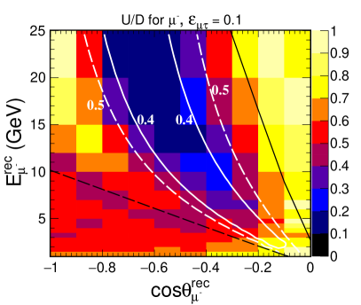
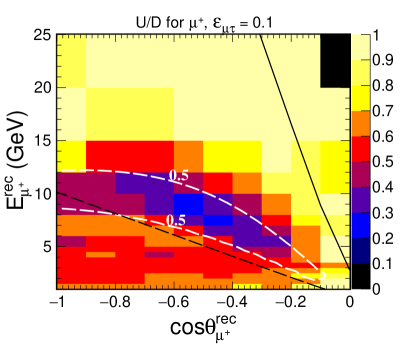
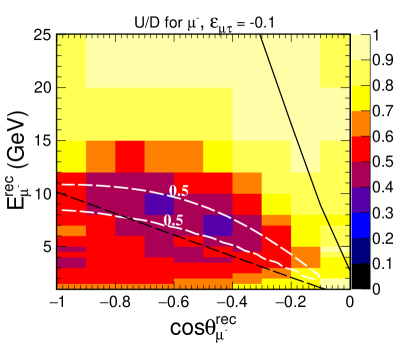
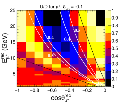
Figure 10: The distributions of U/D ratio in ($E_{\mu}^{\rm rec}$, $\cos\theta_{\mu}^{\rm rec}$) plane with non-zero $|\varepsilon_{\mu\tau}|$ (+0.1 in upper panels and -0.1 in lower panels) as expected at ICAL in 10 years. Left and right panels are for $\mu^{-}$ and $\mu^{+}$ events respectively. The white solid and dashed lines correspond to contours with fitted U/D ratio equal to 0.4 and 0.5, respectively, obtained after fitting of the oscillation valley with function $F_{\alpha}$ (see Eq. 24). The black solid and dashed lines correspond to $\log_{10}[L_{\mu}^{\text{rec}}/E_{\mu}^{\text{rec}}]=$ 2.2 and 3.1, respectively. We consider normal mass ordering, and the benchmark oscillation parameters given in Table 2.

Fig. 10 presents the distributions of U/D ratios of $\mu^{-}$ and $\mu^{+}$ events separately in the $(E_{\mu}^{\rm rec}\,,\cos\theta_{\mu}^{\rm rec})$ plane, for two non-zero $\varepsilon_{\mu\tau}$ values (i.e. $\pm 0.1$). For the sake of demonstration (in order to reduce the statistical fluctuations in the figure and emphasize the physics), we show the binwise average of 100 independent data sets, each with 10-year exposure of ICAL. In contrast to the linear nature of oscillation valley with SI ($\varepsilon_{\mu\tau}=0$), the valley is curved in the presence of NSI. The direction of bending of the oscillation valley is decided by sign of $\varepsilon_{\mu\tau}$ as well as whether it is $\mu^{-}$ or $\mu^{+}$. An important point to note is that the nature of curvature of the oscillation valley, that we observed in the ($E_{\nu},\cos\theta_{\nu}$) plane with neutrino variables (see Fig. 2) with NSI, is preserved in the reconstructed oscillation valley in the plane of reconstructed muon observables ($E_{\mu}^{\rm rec},\cos\theta_{\mu}^{\rm rec}$). This is due to the excellent energy and angular resolutions of the ICAL detector for muons in the multi-GeV energy range.

We retrieve the information on the bending of the oscillation valley by fitting with an appropriate function, which is a generalization of Eq. 23. We introduce an additional free parameter $\alpha$ that characterizes the curvature of the oscillation valley. The function we propose for fitting the oscillation valley in the presence of $\varepsilon_{\mu\tau}$ is

$$F_{\alpha}(E_{\mu}^{\rm rec},\cos\theta_{\mu}^{\rm rec})=Z_{\alpha}+N_{\alpha}\cos^{2}\left(m_{\alpha}\frac{\cos\theta_{\mu}^{\rm rec}}{E_{\mu}^{\rm rec}}+\alpha\,\cos^{2}\theta_{\mu}^{\rm rec}\right),$$ (24)

where $Z_{\alpha}$, $N_{\alpha}$, $m_{\alpha}$, and $\alpha$ are the free parameters to be determined from the fitting of the U/D ratio in the ($E_{\mu}^{\rm rec},\,\cos\theta_{\mu}^{\rm rec}$) plane. Equation 24 is inspired by the survival probability as given in Eq. 9. In Eq. 24, the parameter $\alpha$ enters multiplied with $\cos^{2}\theta_{\mu}^{\rm rec}$, where one factor of $\cos\theta_{\mu}^{\rm rec}$ includes the $L$ dependence of oscillation. The other factor of $\cos\theta_{\mu}^{\rm rec}$ is to take into account the baseline dependence of the matter potential. While this is a rather crude approximation, it is sufficient to provide us a way of calibrating $\varepsilon_{\mu\tau}$, as will be seen later in the section. In Eq. 24, the parameters $Z_{\alpha}$ and $N_{\alpha}$ fix the depth of valley, while $m_{\alpha}$ and $\alpha$ determine the orientation and curvature of oscillation valley, respectively. Therefore, $m_{\alpha}$ and $\alpha$ together account for the combined effect of the mass-squared difference $\Delta m^{2}_{32}$ and the NSI parameter $\varepsilon_{\mu\tau}$ in oscillations.

As in the analysis in Sec. 5, we restrict the range of $\log_{10}[L_{\mu}^{\text{rec}}/E_{\mu}^{\text{rec}}]$ to 2.2 – 3.1, to remove the unoscillated part ($<2.2$) as well as the region with significant matter effects ($>3.1$). The cut on the U/D value is applied at 0.9. In Fig. 10, the contours of the fitted U/D ratio of 0.4 and 0.5, shown with white solid and dashed lines, respectively, clearly indicate that the function $F_{\alpha}$ works well to reproduce the curved nature of the oscillation valley with non-zero $\varepsilon_{\mu\tau}$. We see that the oscillation valley for $\mu^{-}$ with positive (negative) $\varepsilon_{\mu\tau}$ closely resembles that for $\mu^{+}$ with negative (positive) $\varepsilon_{\mu\tau}$. This happens due to the degeneracy in the sign of $\varepsilon_{\mu\tau}$ and the sign of matter potential $V_{\rm CC}$ – these appear in the combination $\varepsilon_{\mu\tau}V_{\rm CC}$ in the survival probability expression in Eq. 9. One can see that for $\mu^{+}$ ($\mu^{-}$) with $\varepsilon_{\mu\tau}=0.1$ ($-0.1$), the contour with the fitted U/D ratio of 0.4 is absent. This is because the valley is shallower in these cases. This feature corresponds to a similar one observed in Fig. 5, where the oscillation dip is shallower for $\mu^{+}$ ($\mu^{-}$) with $\varepsilon_{\mu\tau}=0.1$ ($-0.1$).

6.2 Constraints on $\varepsilon_{\mu\tau}$ from oscillation valley

We saw in the previous section that the shape of the oscillation valley in the muon observables is well-approximated by the function in Eq. 24, with the two parameters $\alpha$ and $m_{\alpha}$. Therefore, we propose to use these two parameters for retrieving $\varepsilon_{\mu\tau}$. At ICAL, since the data on $\mu^{-}$ and $\mu^{+}$ events are available separately, we can have two independent fits for the U/D ratios in $\mu^{-}$ and $\mu^{+}$ events. This would give us independent determinations of the parameter pairs $(\alpha^{-},m_{\alpha}^{-})$ and $(\alpha^{+},m_{\alpha}^{+})$, for $\mu^{-}$ and $\mu^{+}$ events, respectively. One can then get the calibration of $\varepsilon_{\mu\tau}$ in the plane of $\alpha$ and $m_{\alpha}$, for $\mu^{-}$ and $\mu^{+}$ events, separately. For other experiments that do not have charge identification capability, there would be a single calibration curve of $\varepsilon_{\mu\tau}$ with $\alpha$ and $m_{\alpha}$, based on the U/D ratio of muon events without charge information.

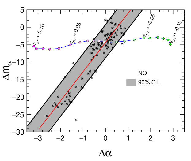
Figure 11: The blue curve with colored circles shows the calibration of $\varepsilon_{\mu\tau}$ in the $(\Delta\alpha,\Delta m_{\alpha})$ plane, obtained from 1000-year MC. The black stars are the values of $(\Delta\alpha,\Delta m_{\alpha}$) obtained from 100 independent data sets, each for 10 years data of ICAL, when $\varepsilon_{\mu\tau}=0$. The gray band represents the expected 90% C.L. region in this plane for a 10-year exposure at ICAL, when $\varepsilon_{\mu\tau}=0$. The part of the blue calibration line covered by the gray band gives the expected 90% C.L. bounds on $\varepsilon_{\mu\tau}$. We consider normal mass ordering, and the benchmark oscillation parameters given in Table 2.

Building up on our experience in the analysis of the oscillation dip in the presence of NSI (see Sec. 4.1), in this analysis of oscillation valley, we use the following observables that quantify the $\mu^{-}$ vs. $\mu^{+}$ contrast in the values of the parameters $\alpha$ and $m_{\alpha}$:

$$\Delta\alpha=\alpha^{-}-\alpha^{+}\,,\hskip 28.45274pt\Delta m_{\alpha}=m_{\alpha^{-}}-m_{\alpha^{+}}\,.$$ (25)

The blue line with colored circles in Fig. 11 shows the calibration of $\varepsilon_{\mu\tau}$ in ($\Delta\alpha,\,\Delta m_{\alpha}$) plane, obtained by using the 1000-year MC sample. It may be observed that the calibration of $\varepsilon_{\mu\tau}$ is almost independent of $\Delta m_{\alpha}$, and $\varepsilon_{\mu\tau}$ is almost linearly proportional to $\Delta\alpha$.

In order to estimate the extent to which $\varepsilon_{\mu\tau}$ may be constrained at ICAL with an exposure of 10 years, we simulate the statistical fluctuations by generating 100 independent data sets, each corresponding to 10-year exposure and $\varepsilon_{\mu\tau}=0$. The black dots in Fig. 11 are the values of $\Delta\alpha$ and $\Delta m_{\alpha}$ determined from each of these data sets. The figure shows the results, with the benchmark oscillation parameters in Table 2.

It is observed that with a 10-year data, the statistical fluctuations lead to a strong correlation between the values of $\Delta\alpha$ and $\Delta m_{\alpha}$, and we have to employ a two-dimensional fitting procedure. We fit the scattered points in $(\Delta\alpha$, $\Delta m_{\alpha}$) plane with a straight line. The best fitted straight line is shown by the red color in Fig. 11, which corresponds to the average of these points, and indeed passes through the calibration point obtained from 1000-year MC events for $\varepsilon_{\mu\tau}=0$. The 90$\%$ C.L. limit on $\varepsilon_{\mu\tau}$ is then obtained based on the measure of the perpendicular distance of every point from the red line. The region with the gray band in Fig. 11 contains 90% of the points that are closest to the red line. The expected 90% C.L. bounds on $\varepsilon_{\mu\tau}$ can then be determined from the part of the blue calibration line covered by the gray band. Any value of the pair $(\Delta\alpha,\Delta m_{\alpha})$ that lies outside the gray band would be a smoking gun signature for nonzero $\varepsilon_{\mu\tau}$ at 90$\%$ C.L. Figure  11 indicates that if $\varepsilon_{\mu\tau}$ is indeed zero, our method, as applied at the ICAL detector, would be able to constrain it to the range $-0.022<\varepsilon_{\mu\tau}<0.021$ at 90% C.L., with an exposure of 500 kt$\cdot$yr.

We explore the possible dilution of our results due to the uncertainties in oscillation parameters and the five systematic errors, following the same procedure described in Sec. 4.2. This yields the expected 90% C.L. bounds as $-0.024<\varepsilon_{\mu\tau}<0.020$, thus keeping them almost unchanged.

7 Summary and Concluding Remarks

Atmospheric neutrino experiments are suitable for exploring the non-standard interactions of neutrinos due to the accessibility to high energies ($E_{\nu}$) and long baselines ($L_{\nu}$) through the Earth, for which the effect of NSI-induced matter potential is large. The NSI matter potential produced in the interactions of neutrino and matter fermions may change the oscillation pattern. The multi-GeV neutrinos, in particular, offer the advantage to access the interplay of NSI and Earth matter effects. In this paper, we have explored the impact of the NSI parameter $\varepsilon_{\mu\tau}$ on the dip and valley patterns in neutrino oscillation probabilities, and proposed a new method for extracting information on $\varepsilon_{\mu\tau}$ from the atmospheric neutrino data.

Detectors like ICAL, that have good reconstruction capability for the energy, direction, and charge of muons, can reproduce the neutrino oscillation dip and valley patterns in their reconstructed muon data, from $\mu^{-}$ and $\mu^{+}$ events separately. The observables chosen to reproduce these patterns are the ratios of upward-going (U) and downward-going (D) events, which minimize the effects of systematic uncertainties. We analyze the U/D ratio in bins of reconstructed muon observables $L_{\mu}^{\rm rec}/E_{\mu}^{\rm rec}$, and in the two-dimensional plane $(E_{\mu}^{\rm rec},\cos\theta_{\mu}^{\rm rec})$. We show that nonzero $\varepsilon_{\mu\tau}$ shifts the locations of oscillation dips in the reconstructed $\mu^{-}$ and $\mu^{+}$ data in opposite directions in the $L_{\mu}^{\rm rec}/E_{\mu}^{\rm rec}$ distributions. At the same time, nonzero $\varepsilon_{\mu\tau}$ manifests itself in the curvatures of the oscillation valleys in the $(E_{\mu}^{\rm rec},\cos\theta_{\mu}^{\rm rec})$ plane, this bending being in opposite directions for $\mu^{-}$ and $\mu^{+}$ events. The direction of shift in the dip location and the direction of the bending of the valley also depend on the sign of $\varepsilon_{\mu\tau}$, as well as on the mass ordering. ICAL, therefore, will be sensitive to sgn($\varepsilon_{\mu\tau}$), once we know the neutrino mass ordering. We present our results in the normal mass ordering scenario, the analysis for the inverted mass ordering scenario will be exactly analogous.

In the oscillation dip analysis, we introduce a new observable $\Delta d$, corresponding to the difference in the locations of dips in $\mu^{-}$ and $\mu^{+}$ event distribution. We show the calibration of $\varepsilon_{\mu\tau}$ against $\Delta d$ using 1000-year MC sample at ICAL, and demonstrate that it is almost independent of the actual value of $\Delta m^{2}_{32}$. We incorporate the effects of statistical fluctuations corresponding to 10-year simulated data, uncertainties in the neutrino oscillation parameters, and major systematic errors, by simulating multiple data sets. Including all these features, it is possible to constrain the NSI parameter in the range $-0.025<\varepsilon_{\mu\tau}<0.024$ at 90% C.L. with 500 kt$\cdot$yr exposure.

In the oscillation valley analysis, we propose a function $F_{\alpha}$ that quantifies the curvature ($\alpha$) and orientation ($m_{\alpha}$) of the oscillation valley in the ($E_{\mu}^{\rm rec}$, $\cos_{\mu}^{\rm rec}$) plane. This analysis may be performed for the $\mu^{-}$ and $\mu^{+}$ events separately, leading to independent measurements of $\varepsilon_{\mu\tau}$. However, we further find that the differences in these parameters for the $\mu^{-}$ and $\mu^{+}$ events are quantities that are sensitive to $\varepsilon_{\mu\tau}$, and show the calibration for $\varepsilon_{\mu\tau}$ in the $(\Delta\alpha,\Delta m_{\alpha})$ plane using 1000-year MC sample at ICAL. Incorporating the effects of statistical fluctuations, uncertainties in the neutrino oscillation parameters, and major systematic errors, the NSI parameter can be constrained in the range $-0.022<\varepsilon_{\mu\tau}<0.021$ at 90% C.L. with 500 kt$\cdot$yr exposure.

A special case of the function $F_{\alpha}$, with $\alpha=0$, corresponds to a valley without any curvature. It is found that the method of fitting for this function $F_{0}$ to the U/D ratio in the ($E_{\mu}^{\rm rec}$, $\cos_{\mu}^{\rm rec}$) plane leads to a more robust and precise measurement of the value of $\Delta m^{2}_{32}$ than the method proposed earlier Kumar:2020wgz .

Our analysis procedure is quite straightforward and transparent, and is able to capture the physics of the NSI effects on muon observables quite efficiently. It builds upon the major features of the impact of $\varepsilon_{\mu\tau}$ on the oscillation dip, and identifies the contrast in the shift in dip locations of $\mu^{-}$ and $\mu^{+}$ as the key observable that would be sensitive to NSI. It exploits the major pattern in the complexity of the two-dimensional event distributions in the ($E_{\mu}^{\rm rec}$, $\cos_{\mu}^{\rm rec}$) plane by fitting to a function approximately describing the curvature of the valley. The two complementary methods of using the oscillation dips and valleys provide a check of the robustness of the results. The shift of the dip location and the bending of the oscillation valley, and survival of these effects in the reconstructed muon data, are deep physical insights obtained through the analysis in this paper.

Note that, though the dip and the valley both arise from the first oscillation minimum, the information content in the valley analysis is more than that in the dip analysis. For example, (a) the features of the valley (like curvature) in Fig. 10 cannot be predicted from the shift in the dip as seen in Fig. 5, and (b) the shift in the dip may have many possible sources, but the specific nature of bending of the valley would act as the confirming evidence for NSI. Therefore, physics unravelled from the valley analysis is much richer than that from the dip.

Note that muon charge identification plays a major role in our analysis. In a detector like ICAL, the measurement of $\varepsilon_{\mu\tau}$ is possible independently in both the $\mu^{-}$ and $\mu^{+}$ channels. The oscillation dips and valleys in $\mu^{-}$ and $\mu^{+}$ event samples have different locations and shapes. As a result, the information available in the dip and valley would be severely diluted in the absence of muon charge identification. But more importantly, the quantities sensitive to $\varepsilon_{\mu\tau}$ in a robust way turn out to be the ones that reflect the differences in the properties of oscillation dips and valleys in $\mu^{-}$ and $\mu^{+}$ events. For example, $\Delta d$ is the observable identified by us, whose calibration against $\varepsilon_{\mu\tau}$ is almost independent of the actual value of $\Delta m^{2}_{32}$. For $\Delta d$ to be measured at a detector, the muon charge identification capability is necessary. The data from ICAL will thus provide the measurement of a crucial observable that is not possible at other large atmospheric neutrino experiments like Super-K or DeepCore/ IceCube. At future long-baseline experiment like DUNE, that will have access to 1 – 10 GeV neutrino energy and separate data sets for neutrino and antineutrino, our methodology to probe NSI using oscillation-dip location can also be adopted, by replacing the U/D ratio with the ratio of observed number of events and the predicted number of events without oscillations.

We expect that further exploration of the features of the oscillation dips and valleys, observable at ICAL-like experiments, would enable us to probe neutrino properties in novel ways.

Acknowledgments

This work is performed by the members of the INO-ICAL collaboration to suggest a new approach to probe Non-Standard Interactions (NSI) using atmospheric neutrino experiments which can distinguish between neutrino and antineutrino events. We thank S. Uma Sankar, Srubabati Goswami, and D. Indumathi for their useful and constructive comments on our work. We thank P. Denton, S. Petcov, G. Rajasekaran. and J. Salvado for useful communications. A. Kumar would like to thank the organizers of the virtual Mini-Workshop on Neutrino Theory at Fermilab, Chicago, USA during 21st to 23rd September, 2020 for giving an opportunity to present the main results of this work. A.K. would also like to thank the organizers of the XXIV DAE-BRNS High Energy Physics Online Symposium at NISER, Bhubaneswar, India during 14th to 18th December, 2020 for providing him an opportunity to give a talk based on this work. We acknowledge support of the Department of Atomic Energy (DAE), Government of India, under Project Identification No. RTI4002. S.K.A. is supported by the DST/INSPIRE Research Grant [IFA-PH-12] from the Department of Science and Technology (DST), India and the Young Scientist Project [INSA/SP/YSP/144/2017/1578] from the Indian National Science Academy (INSA). S.K.A. acknowledges the financial support from the Swarnajayanti Fellowship Research Grant (No. DST/SJF/PSA-05/2019-20) provided by the DST, Govt. of India and the Research Grant (File no. SB/SJF/2020-21/21) provided by the Science and Engineering Research Board (SERB) under the Swarnajayanti Fellowship by the DST, Govt. of India.

References

- (1) Particle Data Group Collaboration, P. Zyla et al., Review of Particle Physics, PTEP 2020 (2020), no. 8 083C01.
- (2) L. Wolfenstein, Neutrino Oscillations in Matter, Phys.Rev. D17 (1978) 2369–2374.
- (3) J. Valle, Resonant Oscillations of Massless Neutrinos in Matter, Phys. Lett. B 199 (1987) 432–436.
- (4) M. Guzzo, A. Masiero, and S. Petcov, On the MSW effect with massless neutrinos and no mixing in the vacuum, Phys. Lett. B 260 (1991) 154–160.
- (5) M. M. Guzzo, H. Nunokawa, P. C. de Holanda, and O. L. G. Peres, On the massless ’just-so’ solution to the solar neutrino problem, Phys. Rev. D64 (2001) 097301, [hep-ph/0012089].
- (6) P. Huber and J. W. F. Valle, Nonstandard interactions: Atmospheric versus neutrino factory experiments, Phys. Lett. B523 (2001) 151–160, [hep-ph/0108193].
- (7) A. M. Gago, M. M. Guzzo, P. C. de Holanda, H. Nunokawa, O. L. G. Peres, V. Pleitez, and R. Zukanovich Funchal, Global analysis of the postSNO solar neutrino data for standard and nonstandard oscillation mechanisms, Phys. Rev. D65 (2002) 073012, [hep-ph/0112060].
- (8) F. J. Escrihuela, M. Tortola, J. W. F. Valle, and O. G. Miranda, Global constraints on muon-neutrino non-standard interactions, Phys. Rev. D83 (2011) 093002, [arXiv:1103.1366].
- (9) M. Gonzalez-Garcia, M. Maltoni, and J. Salvado, Testing matter effects in propagation of atmospheric and long-baseline neutrinos, JHEP 1105 (2011) 075, [arXiv:1103.4365].
- (10) T. Ohlsson, Status of non-standard neutrino interactions, Rept. Prog. Phys. 76 (2013) 044201, [arXiv:1209.2710].
- (11) M. C. Gonzalez-Garcia and M. Maltoni, Determination of matter potential from global analysis of neutrino oscillation data, JHEP 09 (2013) 152, [arXiv:1307.3092].
- (12) Y. Farzan and M. Tortola, Neutrino oscillations and Non-Standard Interactions, Front.in Phys. 6 (2018) 10, [arXiv:1710.09360].
- (13) O. G. Miranda and H. Nunokawa, Non standard neutrino interactions: current status and future prospects, New J. Phys. 17 (2015), no. 9 095002, [arXiv:1505.06254].
- (14) P. S. Bhupal Dev et al., Neutrino Non-Standard Interactions: A Status Report, in NTN Workshop on Neutrino Non-Standard Interactions St Louis, MO, USA, May 29-31, 2019, 2019. arXiv:1907.00991.
- (15) S. K. Agarwalla, S. Das, M. Masud, and P. Swain, Evolution of Neutrino Mass-Mixing Parameters in Matter with Non-Standard Interactions, arXiv:2103.13431.
- (16) M. C. Gonzalez-Garcia and M. Maltoni, Atmospheric neutrino oscillations and new physics, Phys. Rev. D70 (2004) 033010, [hep-ph/0404085].
- (17) I. Mocioiu and W. Wright, Non-standard neutrino interactions in the mu–tau sector, Nucl.Phys. B893 (2015) 376–390, [arXiv:1410.6193].
- (18) J. Kopp, M. Lindner, T. Ota, and J. Sato, Non-standard neutrino interactions in reactor and superbeam experiments, Phys. Rev. D77 (2008) 013007, [arXiv:0708.0152].
- (19) I. Esteban, M. Gonzalez-Garcia, M. Maltoni, I. Martinez-Soler, and J. Salvado, Updated Constraints on Non-Standard Interactions from Global Analysis of Oscillation Data, JHEP 08 (2018) 180, [arXiv:1805.04530].
- (20) A. Esmaili and A. Y. Smirnov, Probing Non-Standard Interaction of Neutrinos with IceCube and DeepCore, JHEP 06 (2013) 026, [arXiv:1304.1042].
- (21) J. Salvado, O. Mena, S. Palomares-Ruiz, and N. Rius, Non-standard interactions with high-energy atmospheric neutrinos at IceCube, JHEP 01 (2017) 141, [arXiv:1609.03450].
- (22) IceCube Collaboration, M. Aartsen et al., Search for Nonstandard Neutrino Interactions with IceCube DeepCore, Phys. Rev. D97 (2018), no. 7 072009, [arXiv:1709.07079].
- (23) Super-Kamiokande Collaboration, G. Mitsuka et al., Study of Non-Standard Neutrino Interactions with Atmospheric Neutrino Data in Super-Kamiokande I and II, Phys.Rev. D84 (2011) 113008, [arXiv:1109.1889].
- (24) S. Choubey, A. Ghosh, T. Ohlsson, and D. Tiwari, Neutrino Physics with Non-Standard Interactions at INO, JHEP 12 (2015) 126, [arXiv:1507.02211].
- (25) A. Khatun, S. S. Chatterjee, T. Thakore, and S. Kumar Agarwalla, Enhancing sensitivity to non-standard neutrino interactions at INO combining muon and hadron information, Eur. Phys. J. C 80 (2020), no. 6 533, [arXiv:1907.02027].
- (26) ICAL Collaboration, S. Ahmed et al., Physics Potential of the ICAL detector at the India-based Neutrino Observatory (INO), Pramana 88 (2017), no. 5 79, [arXiv:1505.07380].
- (27) India-based Neutrino Observatory (INO), http://www.ino.tifr.res.in/ino/.
- (28) S. Mikheev and A. Y. Smirnov, Resonant amplification of neutrino oscillations in matter and solar neutrino spectroscopy, Nuovo Cim. C9 (1986) 17–26.
- (29) S. Mikheev and A. Y. Smirnov, Resonance Amplification of Oscillations in Matter and Spectroscopy of Solar Neutrinos, Sov.J.Nucl.Phys. 42 (1985) 913–917.
- (30) P. Huber, M. Lindner, and W. Winter, Superbeams versus neutrino factories, Nucl.Phys. B645 (2002) 3–48, [hep-ph/0204352].
- (31) G. L. Fogli, E. Lisi, A. Marrone, D. Montanino, A. Palazzo, and A. M. Rotunno, Solar neutrino oscillation parameters after first KamLAND results, Phys. Rev. D67 (2003) 073002, [hep-ph/0212127].
- (32) A. Kumar, A. Khatun, S. K. Agarwalla, and A. Dighe, From oscillation dip to oscillation valley in atmospheric neutrino experiments, Eur. Phys. J. C 81 (2021), no. 2 190, [arXiv:2006.14529].
- (33) Super-Kamiokande Collaboration, Y. Ashie et al., A Measurement of atmospheric neutrino oscillation parameters by Super-Kamiokande I, Phys.Rev. D71 (2005) 112005, [hep-ex/0501064].
- (34) IceCube Collaboration, M. Aartsen et al., Energy Reconstruction Methods in the IceCube Neutrino Telescope, JINST 9 (2014) P03009, [arXiv:1311.4767].
- (35) N. Dash, V. M. Datar, and G. Majumder, A Study on the time resolution of Glass RPC, arXiv:1410.5532.
- (36) A. D. Bhatt, V. M. Datar, G. Majumder, N. K. Mondal, Pathaleswar, and B. Satyanarayana, Improvement of time measurement with the INO-ICAL resistive plate chambers, JINST 11 (2016), no. 11 C11001.
- (37) A. Gaur, A. Kumar, and M. Naimuddin, Study of timing response and charge spectra of glass based Resistive Plate Chamber detectors for INO-ICAL experiment, JINST 12 (2017), no. 03 C03081.
- (38) M. Sajjad Athar, M. Honda, T. Kajita, K. Kasahara, and S. Midorikawa, Atmospheric neutrino flux at INO, South Pole and Pyhásalmi, Phys.Lett. B718 (2013) 1375–1380, [arXiv:1210.5154].
- (39) M. Honda, M. S. Athar, T. Kajita, K. Kasahara, and S. Midorikawa, Atmospheric neutrino flux calculation using the nrlmsise-00 atmospheric model, Phys. Rev. D 92 (Jul, 2015) 023004.
- (40) D. Casper, The Nuance neutrino physics simulation, and the future, Nucl.Phys.Proc.Suppl. 112 (2002) 161–170, [hep-ph/0208030].
- (41) A. Chatterjee, K. Meghna, K. Rawat, T. Thakore, V. Bhatnagar, et al., A Simulations Study of the Muon Response of the Iron Calorimeter Detector at the India-based Neutrino Observatory, JINST 9 (2014) P07001, [arXiv:1405.7243].
- (42) N. Dash, Feasibility studies for the detection of exotic particles using ICAL at INO. PhD thesis, HBNI, Mumbai, 2015.
- (43) S. Pal, Development of the INO-ICAL detector and its physics potential. PhD thesis, HBNI, Mumbai, 2014.
- (44) P. de Salas, D. Forero, S. Gariazzo, P. Martínez-Miravé, O. Mena, C. Ternes, M. Tórtola, and J. Valle, 2020 Global reassessment of the neutrino oscillation picture, arXiv:2006.11237.
- (45) I. Esteban, M. Gonzalez-Garcia, M. Maltoni, T. Schwetz, and A. Zhou, The fate of hints: updated global analysis of three-flavor neutrino oscillations, JHEP 09 (2020) 178, [arXiv:2007.14792].
- (46) F. Capozzi, E. Di Valentino, E. Lisi, A. Marrone, A. Melchiorri, and A. Palazzo, Global constraints on absolute neutrino masses and their ordering, Phys. Rev. D 95 (2017), no. 9 096014, [arXiv:2003.08511]. [Addendum: Phys.Rev.D 101, 116013 (2020)].
- (47) NuFIT webpage, http://www.nu-fit.org/.