Uncertainties in Galaxy Rotation Curves

Abstract

Assessing the likelihood that the rotation curve of a galaxy matches predictions from galaxy formation simulations requires that the uncertainties in the circular speed as a function of radius derived from the observational data be statistically robust. Few uncertainties presented in the literature meet this requirement. In this paper we present a new standalone tool, makemap, that estimates the fitted velocity at each pixel from Gauss-Hermite fits to a 3D spectral data cube, together with its uncertainty obtained from a modified bootstrap procedure. We apply this new tool to neutral hydrogen spectra for 18 galaxies from the THINGS sample, and present new velocity maps with uncertainties. We propagate the estimated uncertainties in the velocity map into our previously-described model fitting tool DiskFit to derive new rotation curves. The uncertainties we obtain from these fits take into account not only the observational errors, but also uncertainties in the fitted systemic velocity, position of the rotation centre, inclination of the galaxy to the line of sight, and forced non-circular motion. They are therefore much better-defined than values that have previously been available. Our estimated uncertainties on the circular speeds differ from previous estimates by factors ranging up to of five, being smaller in some cases and larger in others. We conclude that kinematic models of well-resolved HI datasets vary widely in their precision and reliability, and therefore potentially in their value for comparisons with predictions from cosmological galaxy formation simulations.

1 Introduction

Galaxy formation simulations (see Somerville & Davé, 2015, for a recent review) are making increasingly detailed predictions for the properties of galaxies to be confronted with data. Much of the recent emphasis has been on chemical evolution and the distribution of metals among the stars and both the cool and hot gas, and plenty of data is coming from surveys such as APOGEE (Majewski et al., 2017) and GALAH (de Silva et al., 2015). However, the structure and mass distribution of disc galaxies remain key predictions of the models (e.g. Buck et al., 2020; Vogelsberger et al., 2020; Wellons et al., 2020) that can be confronted by spectral line observations of galaxies in the local universe. The 21cm line of atomic hydrogen (HI) is particularly useful because the HI disc is typically more extended than the optical galaxy and thus traces the kinematics into the region dominated by dark matter. As a result, there is now a long history of detailed comparisons between the observed rotation curves of nearby galaxies derived from interferometric HI maps and theoretical predictions from galaxy formation models (see de Blok, 2010; Lelli, McGaugh & Schombert, 2016, for reviews).

Much recent discussion has focused on whether or not baryonic effects, such as feedback from star formation, can explain discrepancies between the predicted mass distributions of collisionless cold dark matter halos and the observed rotation curves of nearby galaxies. The slope and scatter of scaling relations built from rotation curve compilations are powerful tools in this regard (Dutton et al., 2007; Lelli, McGaugh & Schombert, 2016; Posti et al., 2019), and it remains unclear whether rotation curve models of individual galaxies are, or are not, consistent with cosmological galaxy formation predictions (e.g. Oh et al., 2011; Oman et al., 2015; Katz et al., 2017; Haghi et al., 2018; Marasco et al., 2020). Some issues raised may be somewhat less affected by baryonic feedback, which is frequently invoked to explain away the cusp/core controversy and other small-scale problems (reviewed by Weinberg et al., 2015).

Properly evaluated uncertainties in the measured circular speeds are required in order to assess the likelihood that a set of observed rotation curves from galaxies is consistent with the predictions of the models. However, such uncertainties have not as yet been derived in a statistically correct manner.

The traditional procedure for deriving a rotation curve from a well-resolved HI data cube of a nearby, intermediate inclination galaxy has been first to create a 2D velocity map and then to fit a tilted ring model to the velocity map (Rogstad, Lockhart & Wright, 1974). The standard tilted ring software, rotcur (Begeman, 1989), assumes the gas to flow on circular orbits. Franx, van Gorkom & de Zeeuw (1994) and Schoenmakers et al. (1997) generalized rotcur to mildly non-circular flows, but their tool, reswri, assumes that the response to potential distortions can be modelled by forced epicycles, and can therefore fit only mildly elliptical streamlines.

The underlying assumption of such models is that the gas is flowing in a thin, possibly warped, layer in centrifugal balance in a nearly axisymmetric potential, and therefore has a well-defined circular speed at every radius in the galaxy disc. Even accepting that these assumptions are true, the fitted circular speed at each radius is affected by the choices for the systemic velocity, the location of the rotation centre, and both the inclination and position angle of the disc plane to the line of sight. Uncertainties in these quantities, as well as beam smearing, turbulence, forced non-axisymmetric flows, and noise in the data, should all contribute to the uncertainty in the estimated circular speed at each radius.

As the resolution and S/N of the observations have improved, the formal statistical uncertainties in both the estimated velocity in each pixel of the 2D map and the fitted circular speed at each radius have become absurdly small, for the reason we give below in §2.2. Because of this, many workers (e.g. Chemin, Carignan & Foster, 2009) present ad hoc error bars on the circular speed estimates at each radius in the galaxy that are based upon the difference between the separately-fitted circular speeds on the approaching and receding sides of the galaxy, while holding the kinematic centre, systemic velocity, and projection angles at their best fit values for the whole map. de Blok et al. (2008) adopt this approach but add in quadrature the dispersion of velocities within the model ring. Although these “error bars” have little statistical validity, they are claimed to be realistic merely because the values are a significant fraction of the fitted circular speed and are generally larger where the model is a poorer fit.

Several algorithms are now publicly-available that analyze the 3D spectral cube directly rather than 2D velocity fields (Kamphuis et al., 2015; Di Teodoro & Fraternali, 2015; Davis et al., 2013, 2020), building on earlier development by Jòzsa et al. (2007). This approach is particularly useful for comparing complex models to deep, very well-resolved HI data (Jòzsa et al., 2009; Kamphuis et al., 2013; Marasco et al., 2019) or for lower resolution data in which beam smearing in 2D maps can be severe (Di Teodoro & Fraternali, 2015; Kamphuis et al., 2015). In principle, 3D models constrain HI spectral data more directly than their 2D counterparts and avoid the need to first derive a 2D velocity field. But in practice most apply the same iterative approach of the classic 2D rotcur/reswri algorithm (Sicking, 1997; Schoenmakers et al., 1997) as has long been done in 2D, and suffer from the same shortcomings as described above. Uncertainties returned by frequentist codes generally stem from ad hoc variations of model parameters (e.g. Kamphuis et al., 2015; Di Teodoro & Fraternali, 2015), and there is a need to explore whether the posterior distributions of Bayesian methods (e.g. Bouché et al., 2015; Davis et al., 2017) better reflect uncertainties in the fit. In addition, performance tests on well-resolved datasets have revealed that 3D codes converge much more slowly to the same fitting parameters as are found from 2D velocity maps. 3D methods are therefore impractical in this regime and there remains a need for statistically robust techniques to derive and analyze 2D velocity maps from 3D HI spectral cubes.

As already noted, fitting an idealized circular flow pattern to a 2D kinematic map neglects the possible existence of coherent turbulence or noncircular motions forced by spiral arms and the like (Oman et al., 2019). Thus the residuals after subtracting a circular flow model contain correlations that cannot be accounted for in the formal statistical errors of the model parameters. The advantages of the DiskFit software (Sellwood & Spekkens, 2015) over rotcur are two fold: (1) it can fit for bar-like flows and (2) it also estimates uncertainties in all fitted parameters and the fitted velocities at each radius. The modified bootstrap procedures described by Spekkens & Sellwood (2007) and Sellwood & Zánmar Sánchez (2010) to estimate all uncertainties not only take account of the large-scale correlations in the pattern of residuals after subtracting a fitted smooth model from the velocity map but also factor in uncertainties in the global parameters. It should be noted that the uncertainties yielded by their procedures seemed reasonable, but these authors did not attempt to prove that they were large enough or statistically meaningful.

However, uncertainties in the fitted velocity at each pixel of the velocity map are generally unavailable for neutral hydrogen data, and therefore cannot be propagated into the uncertainties in the rotation curve. When this is the case, DiskFit adopts a fixed uncertainty, $\Delta_{\rm ISM}$, whose value is chosen by the user. Values in the range $8\la\Delta_{\rm ISM}\la 12\;$km s^-1 would be consistent with the observed turbulent motions of gas in the ISM of a large star forming disc galaxy (Gunn, Knapp & Tremaine, 1979; Kamphuis, 1993). This choice is motivated by the reasoning that the velocity fitted to the spectrum may be dominated by emission from material whose velocity may differ from the circular speed by this much. However, an assumption of a uniform uncertainty in the fitted velocity of each pixel is clearly inadequate, since it gives equal weight in the fitted model to pixels at which the velocity is well-determined and to those where the fitted velocity is poorly constrained.

While bootstrap iterations in DiskFit yield uncertainties in the fitted parameters and velocities, it would be better to begin with a velocity map that also has an associated uncertainty for the line-of-sight velocity at each pixel. Once velocity errors in each pixel of the map are in hand, they can be propagated all through the fitting process to yield more statistically meaningful uncertainties in the derived projection parameters and circular speed at each radius, as we describe in §3.3.

In §2, we describe a new standalone program, makemap, that derives a 2D velocity map from a 3D data cube. It uses a modified bootstrap method to estimate the uncertainties in the velocity at each pixel. We distribute it as an addition to the DiskFit package (Sellwood & Spekkens, 2015). There seems no reason, in principle, why the modification to the bootstrap method we develop here could not be employed in other packages that attempt to extract the rotation curve directly from the data cube.

We apply makemap to 18 publicly available data cubes of HI emission from galaxies in the THINGS survey (Walter et al., 2008). From each data cube, we extract a 2D velocity map together with a map of the uncertainty in the estimated velocity at each pixel, and input the derived maps to DiskFit to obtain new rotation curves having uncertainties that are better-determined.

2 Making a map

This section introduces program makemap, which fits a smooth Gauss-Hermite function to the line profile in each velocity column of the data cube that appears to contain significant spectral line emission. We use a modified bootstrap approach to estimate uncertainties for the fitted line parameters. In this section we illustrate our procedure using the THINGS data cube for NGC 2841; we apply makemap to 18 THINGS galaxies in §4.

A number of different methods have been employed to derive a 2D velocity map from a 3D data cube, which also differ between optical and radio data. On the one hand, the spectral resolution of HI emission line data is high enough that individual velocity channels are statistically independent, something that is not usually true for optical data from a Fabry-Pérot system or a fibre bundle, say. On the other hand, the spatial resolution of optical data is generally high enough that adjacent pixels are independent, or nearly so, while the beam size in radio data generally extends over a number of pixels. Here we focus on HI data from interferometers, and leave applications of the ideas we develop to CO data or to optical data to later papers.

The intensity-weighted mean velocity, also known as the first moment, is one possible estimate of the gas velocity, and the THINGS team (Walter et al., 2008) have posted moment 1 maps of all the galaxies in that sample on their website. Some workers (e.g. Gentile et al., 2006) trace the envelope of the line profile to find the velocity of peak emission. Others (e.g. Ponomareva et al., 2016) fit a single Gaussian to the line profile, adopting the peak of the fitted function as the derived velocity. Oh et al. (2008, 2019) fit multiple Gaussians to try to separate side peaks, which they attribute to random motions, from the “bulk” velocity. de Blok et al. (2008, hereafter dB08) fitted a generalized Gaussian (Gerhard, 1993; van der Marel & Franx, 1993), which has the advantage that it takes account of the possible skewness of the line profile that can be significant, especially for large beam sizes and when the galaxy is not far from edge-on. dB08 presented two examples to illustrate the differences between the velocity estimated by their new method and those obtained by the other procedures. Since the formal statistical uncertainty in the fitted velocity at each pixel in the map is always much smaller than the likely turbulent dispersion, many authors neglect velocity uncertainties altogether.

2.1 Line fitting

Following dB08, we fit a Gauss-Hermite function to the measured intensity as a function of velocity for each pixel in the data cube. Assuming only $h_{3}$ and $h_{4}$ are non-zero, van der Marel & Franx (1993, their eq. (9)) write the “line profile” as

$${\cal L}(v)={\cal L}_{0}+\left[{A\alpha(w)\over\sigma}\right]\left\{1+h_{3}H_{3}(w)+h_{4}H_{4}(w)\right\},$$ (1)

where $w=(v-\bar{V})/\sigma$, $H_{3}(w)=w(2w^{2}-3)/\sqrt{3}$, $H_{4}(w)=(4w^{4}-12w^{2}+3)/\sqrt{24}$, and $\alpha(w)=\exp(-w^{2}/2)/\sqrt{2\pi}$. The set of paramaters, $\{p(m)\}$, to be determined is: $p(1)={\cal L}_{0}$ the estimated continuum, $p(2)=A$ the normalization of the line amplitude, $p(3)=\bar{V}$ the central velocity of the fitted profile, $p(4)=\sigma$ an estimate of the line width, and, optionally, $p(5)=h_{3}$ and $p(6)=h_{4}$ the coefficients that quantify departures of the line profile from a simple Gaussian. A skew line profile would be better fitted with a non-zero value of $h_{3}$, while $h_{4}$ would be positive if the profile has heavy tails and negative for a line that is more peaked than a Gaussian; these parameters therefore describe the profile in an analagous, but distinct, manner to the familiar skew and kurtosis parameters (e.g. Press et al., 1992).

It is important to realize that the velocity $V_{m}$ for which expression (1) is maximum is generally not the value of $\bar{V}$ when $h_{3}\neq 0$. We find that $|V_{m}-\bar{V}|\la\sigma/2$ when $|h_{3}|\sim 0.5$. We adopt $V_{m}$ as “the best fit velocity”. Obviously, $V_{m}\equiv\bar{V}$ for a Gaussian function.

Program makemap attempts to fit expression (1) to the set of intensities $\{I(v_{k})\}$ in each spectral column of a data cube, where $\{v_{k}\}$ are the channel velocities that are separated by a fixed $\delta v$, aka the channel width. We generally recommend that the fit includes the $h_{3}$ term only, but the user can choose to fit for both $h_{3}$ and $h_{4}$, or neither (i.e. a simple Gaussian) if desired.

The first step is to estimate the noise level, ${\cal N}$, in the raw data cube, which we assume to be constant. Program makemap uses the bi-weight estimator (Beers, Flynn & Gebhardt, 1990) to compute the mean and dispersion of the intensity values in the outermost 2 layers of all 6 faces of the data cube, and adopts ${\cal N}$ for the entire cube to be this estimated dispersion. The bi-weight is superior to the rms value since it ignores outliers and heavy tails in the distribution of values; see Beers, Flynn & Gebhardt (1990) for a discussion of different distribution width estimators.

Then working over the image plane, program makemap attempts to fit a line profile to $\{I(v_{k})\}$ only when the maximum value of $I(v_{k})>I_{n,\rm min}\times\,{\cal N}$, with $I_{n,\rm min}$ being a constant set by the user.

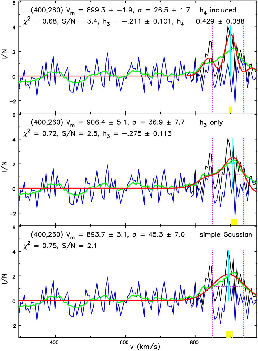
Figure 1: An example of a low S/N line from NGC 2841 to illustrate the behaviour of the fitting program. The bottom panel fits a simple Gaussian ($h_{3}=h_{4}=0$) to the data; that in the middle includes $h_{3}$ only, while the top panel shows the result of fitting for both $h_{3}$ and $h_{4}$. In all three panels, the black jagged line shows the input data $\{I(v_{k})/{\cal N}\}$ in units of the noise, the blue jagged line, which obscures the black line for much of the range, indicates the residuals after subtracting the fitted function, shown by the smooth red curve. The green line is the 10-point running average of $\{\bar{I}_{n}(v_{k})\}$ and the vertical parts of the dotted magenta H illustrate the first guesses at $\bar{V}\pm\sigma$. Finally, the vertical cyan line is the fitted $V_{m}$ and the horizontal error bar shows its estimated uncertainty, while the yellow marks indicate fitted maximum velocity from each of the 20 bootstraps.

Program makemap uses the fitting tool sumsl (from the software collection made public by Burkardt, 2017), which is a quasi-Newton method requiring first derivatives, to find the set of parameters $\{p(m)\}$ that mimimize

$$\chi_{\rm line}^{2}=\sum_{k}\left[I_{n}(v_{k})-{\cal L}(v_{k})\right]^{2},$$ (2)

where now $I_{n}(v_{k})=I(v_{k})/{\cal N}$; because the input data values have been normalized by the noise, this is the usual definition of $\chi^{2}$. This form is appropriate only when the noise level is constant throughout the data cube, as it is for most HI data cubes. To use makemap for cubes having a position and/or channel dependent noise level, one would need to rewrite eq. (2) in standard form.

Starting the minimization from a good first guess helps to prevent the minimizer from finding a local minimum far from the global minimum. In order to choose this guess, makemap first creates a smoothed set of intensities $\bar{I}_{n}(v_{k})$ from a running average of ten $I_{n}(v_{k})$ values and sets the first guesses of $A$ and $\bar{V}$ respectively from the maximum of $\bar{I}_{n}(v_{k})$ and its velocity. The initial guess for $\sigma$ is half the velocity-width of $\bar{I}_{n}(v_{k})$ at half its maximum intensity. The initial guesses for ${\cal L}_{0}$, $h_{3}$, and $h_{4}$ are all zero. Although this procedure would have difficulty in fitting an extremely broad, low S/N line, the sources of such lines are unlikely to be found in galaxy discs. For other applications, we would recommend combining velocity channels before fitting such lines in order to improve S/N.

Figure 1 illustrates the fit for one pixel having low S/N emission in the THINGS data cube for NGC 2841. The bottom panel fits a simple Gaussian ($h_{3}=h_{4}=0$) to the data; that in the middle includes $h_{3}$ only, while the top panel shows the result of fitting for both $h_{3}$ and $h_{4}$. The caption describes the various coloured lines. The fitted parameter values and their uncertainties are recorded in each panel; note that the negative uncertainty in the fitted velocity in the top panel flags the bimodal nature of the fitted function (see §2.3).

Notice that the best fit value of $V_{m}$ differs by almost 13 km/s between the Gaussian fit and that which includes $h_{3}$, which is just about consistent with the combined estimated uncertainties of the two fits. We determine uncertainties as described in §2.2.

The user must choose values for a few parameters to determine whether a line is rejected. They are: $I_{n,\rm min}$, the minimum normalized intensity in the spectrum before a fit is attempted, $A_{\rm min}$, the minimum acceptable line amplitude, $w_{\rm max}$, the maximum allowed line width, and $h_{\rm max}$, the max acceptable absolute value of the Gauss-Hermite coefficients. Tallies of rejected fits are tabulated according to the following fail criteria:

1. The maximum value of $I_{n}(v_{k})<I_{n,\rm min}$,

2. The line fitting routine fails (very rare),

3. The line intensity, in units of ${\cal N}$, $A/(\sqrt{2\pi}\sigma)<A_{\rm min}$,

4. The fitted $\bar{V}$ is outside the range of velocities in the channel maps,

5. The line width $\sigma>w_{\rm max}\,\delta v$. The fit is also rejected when $\sigma<2I_{n,\rm min}\,\delta v/I_{n,\rm max}$, where $I_{n,\rm max}$ is the greatest value of $\{I_{n}(v_{k})\}$. This is to reject low S/N lines, that could be little more than a noise spike in one channel, while retaining high S/N lines that have a narrow width.

6. Either $|h_{3}|>h_{\rm max}$ or $|h_{4}|>h_{\rm max}$,

7. When bootstraps are included (see §2.2 below), one or more iterations has returned nonsensical fitted parameters. To wit, either $A<0$, $\sigma<0$, or $\bar{V}$ is outside the range of velocities in the channel maps. This usually happens only when the S/N is low.

Program makemap reports these tallies, as well as the number of line profiles that were successfully fitted. For every fit that fails, it assigns the default values of zero for all parameters.

We determine the best fit velocity, $V_{m}$, from among the roots of $\partial{\cal L}/\partial v=0$. Rejected fits are assigned the default value $V_{m}=-9999\;$km/s.

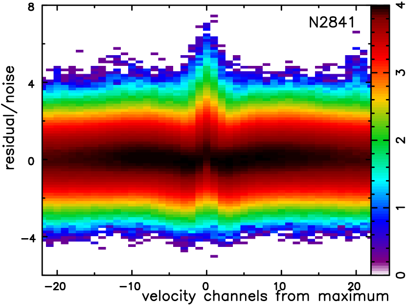
Figure 2: The distributions of residuals from all fitted pixels in the data cube from NGC 2841, in units of the noise, after subtracting the best fit function (1) that included only the $h_{3}$ term. The distribution of residuals in the velocity channels at each pixel is shifted so that the channel with the greatest fitted intensity is at 0. The colour represents the logarithm of the number of pixels having the given value. The distributions of residuals are consistent with noise except for a few channels near the line centre.

2.2 Parameter uncertainties

Program makemap estimates the uncertainty in each fitted parameter by a modified bootstrap method. The user must supply a value for $n_{\rm boot}$, the number of desired bootstrap iterations to be used for each pixel of the map for which the fit was accepted. A value of $n_{\rm boot}\leq 0$ will prevent uncertainties from being estimated.

As noted in §1, the principal obstacle to a satisfactory accounting for errors is that the formal statistical errors in both the fitted velocity at each pixel and the circular speed at each radius are absurdly small. It is instructive to consider why this should be the case.

When fitting a parameterized model to data by mimimizing $\chi^{2}$, MCMC, or any other method, the standard estimators of the parameter uncertainties assume that the data contain no additional information other than the model plus noise or, in other words, $\chi^{2}$ per degree of freedom should be close to unity. When this ideal assumption holds, errors estimated by formal techniques should be meaningful. The assumption that the data are perfectly described by the adopted model plus uncorrelated noise rarely holds in the real world, however, where the model is generally an idealized approximation to the data.

In the case of intensities as a function of velocity in each pixel spectrum of a data cube, the line profile is indeed noisy because of imperfections in the observations, but the net emission from a clumpy, turbulent ISM is most unlikely to have the kind of intrinsically smooth profile that is fitted, and emission from individual clouds must add to the ragged appearance of the data, especially at the velocities close to the line peak. Subtracting a smooth line profile from the data and considering the residuals to be exclusively noise, neglects the intrinsic substructure in the line profile, as was already recognized by Oh et al. (2008, 2019); the true uncertainty in the fitted velocity is increased when substructure is accounted for.

The standard bootstrap strategy to estimate uncertainties is to subtract the fitted function, eq. (1), from the data to create a set of residuals $\{\delta(v_{k})\equiv I_{n}(v_{k})-{\cal L}(v_{k})\}$ at each $v_{k}$, and then make new fits to $n_{\rm boot}$ sets of pseudo data $P(v_{j})$, where $P(v_{j})={\cal L}(v_{j})+\delta^{\prime}(v_{j})$ to find $n_{\rm boot}$ sets of parameters $\{p^{\prime}(m)\}$ and $V_{m}^{\prime}$. At each iteration $\delta^{\prime}(v_{j})$ is a random draw from the pool of $\{\delta(v_{k})\}$. The uncertainty estimate of each parameter is then $ep(m)=\langle[p(m)-p^{\prime}(m)]^{2}\rangle^{1/2}$ and similarly for $eV_{m}$.

This procedure yields the correct uncertainty when the observed line is perfectly described by the adopted function (eq. 1), and the residuals are simply uncorrelated noise. However, the pattern of residuals around the line peak contains some signal that is more than just random noise, as is illustrated in Figure 2. This figure is based upon all 163,676 pixels for which $h_{3}$ only fits to the THINGS data cube from NGC 2841 were accepted. For each pixel, the distribution of residuals, divided by the noise, is shifted in velocity so that the peak of the fitted line is at zero. It is clear that the residuals are somewhat larger on average a few velocity channels from the line centre, consistent with the example in Figure 1.

We therefore adopt a different strategy. We create sets of pseudo data by shifting the pattern of residuals about the peak of the best fit curve while preserving their sequence and values. For $n_{\rm boot}=20$, say, we shift the residual pattern by one channel at a time from $-10$ channels to $+10$ (skipping 0, of course) in a deterministic manner at each iteration and refit. Were the residual pattern simply uncorrelated noise, this strategy would return similar uncertainties in the fitted parameters as for random draws from the pool of residuals, but preserving the intrinsic substructure of the true emission line in this way yields a larger and more realistic uncertainty in the fitted velocity.

Obviously, the value of $n_{\rm boot}$ cannot be larger than the number of channels and should usually be less. We have experimented with different numbers for NGC 2841, and show in Figure 3 that distribution of uncertainties changes very little for $n_{\rm boot}\ga 20$. We have found similar distributions for two other galaxies. However, the median value of $eV_{m}\simeq 2.8\;$km s^-1 in NGC 2841 is small compared with the likely turbulent velocity spread in the gas of any star-forming galaxy.

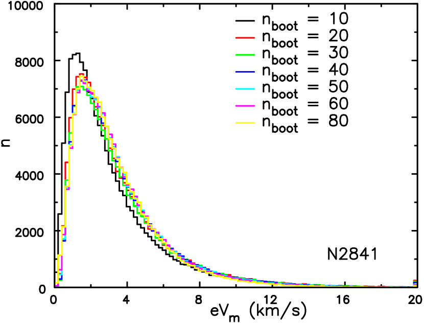
Figure 3: The distributions of $eV_{m}$ from various numbers of bootstraps of fits to the data of NGC 2841 that included only the $h_{3}$ term. The differences for $n_{\rm boot}>10$ are minor.

2.3 Bimodal line profiles

The Gauss-Hermite function (eq. 1) can have two distinct maxima near the line centre when $h_{3}$ and/or $h_{4}$ are non-zero. Two or more peaks in the fitted line profile can arise because of noise or it could imply streams of gas along the line of sight having distinct velocities, which would violate one of the key assumptions implicit when fitting a flow pattern to the data.

Program makemap therefore flags fitted line profiles that are significantly bimodal. It determines whether the smooth function ${\cal L}(v)$ (eq. 1) has multiple maxima and, if so, whether any of the fitted secondary maxima are significant enough for the line to qualify as bimodal. It finds all the roots of $\partial{\cal L}(v)/\partial v=0$ and checks the sign of the second derivative at the position of each root to locate the maxima in the best fit line profile. It discards any secondary maxima that are less than 20% of the greatest, the weaker of two maxima when two are closely spaced, i.e. when $\delta v<\sigma/2$, and cases where the 2nd maximum is scarcely more than inflexion in ${\cal L}(v)$. To identify this last case, the minimum between the two maxima must be deeper than either 80% of the lesser peak or 50% of the average of the two adjacent maxima.

When the number of surviving maxima is greater than one, a line is flagged as bimodal by changing the sign of the uncertainty $eV_{m}$ if $n_{\rm boot}>0$, or by changing the sign of the S/N otherwise. Both these quantities are intrinsically positive, so the flag is unambiguous. For example, the fitted profile in the middle panel of Figure 1 is not bimodal, but the negative value of $eV_{m}$ for the fit in the top panel flags the bimodality.

Oh et al. (2008, 2019) also try to identify bimodal line profiles, but fit a second Gaussian to a side peak, describing the main peak as the “bulk velocity”. This is similar to our definition of the “best fit velocity” $V_{m}$, which is that of the absolute maximum of the smooth line profile (eq. 1). However, these authors adopt the peak they judge to be the bulk velocity as the fitted velocity, whereas we simply record the greatest peak and generally discount lines that are flagged as bimodal.

2.4 Omit $h_{4}$

We caution that when fitting the six-parameter function (eq. 1) to low S/N data, the extra freedom in the fitted function relative to a simple Gaussian could be used to fit a spurious noise peak in addition to the true peak. Figure 1 provides a good illustration of the dangers of giving the fitting program more and more freedom to fit the data. In this case, it is clear that the line fitting program is confused by the spike near 820 km/s which could be real or a $3\sigma$ fluctuation in the noise, and it reports a much smaller uncertainty $eV_{m}$, which is negative to flag the line as bimodal for this fit.

This is one example to illustrate the undesirable consequences of giving the fitting function too much freedom, and we recommend no more than a five-parameter fit, with $h_{4}$ forced to be zero.

3 Application to THINGS

The data available on the THINGS website include moment 0, moment 1 and moment 2 maps, that are blanked outside the mask that the THINGS team defined. The unmasked “standard” cube, in the terminology of Walter et al. (2008), is also available, but their posted moment maps are not created from the standard cube. We work with the “natural weights” data, which have slightly higher sensitivity and lower angular resolution than do the “robust weights” data.

The standard cubes contain the intensities in the 21 cm line after an almost complete data reduction, that includes cleaning of all sources down to a level of 2.5 times the noise. Two steps remain to be performed in order to correct to the actual line fluxes: a rescaling to make an approximate correction for the uncleaned sources caused by the difference between the solid angle of the dirty and clean beams (Jörsäter & van Moorsel, 1995), and a correction for primary beam attentuation. Walter et al. (2008) created the moment maps from the rescaled data cube, in order that the flux in the moment 0 map be the best possible estimate.

However, correcting for both these effects will alter the noise, as well as the signal, in every value in the cube, and a non-uniform level of noise would complicate the fitting of line profiles. The THINGS team provide their “standard” cube, rather than the “rescaled” cube, at least in part because the noise is constant throughout the cube (Walter et al., 2008). In fact, since primary beam attenuation across a narrow frequency range is simply position dependent, correcting for it has no effect on the shape of the line profile in any pixel, and therefore does not change the fitted velocity, as Walter et al. (2008) point out. However, rescaling to correct for the dirty beam of uncleaned sources still present could, in principle, mildly affect the shapes of the line profiles, although the extent to which it could affect the fitted velocity is unclear. With this caveat, both dB08 and ourselves fit line profiles to the standard cube. The estimated noise in every pixel and velocity channel is that given in Table 3 of Walter et al. (2008), and their values are in very good agreement with our bi-weight esimates of the noise from the outer layers of the cube (see §2.1).

Many of the data cubes used in our analysis were also re-analyzed by Ponomareva et al. (2016). They smoothed the THINGS cubes to a common spatial resolution of all their galaxies, rederived velocity maps from Gaussian fits, discarding pixels having strongly skew line profiles, and extracted rotation curves also using rotcur, without estimating uncertainties.

3.1 Masking

It is, of course, possible to attempt to fit a line to every pixel in the cube, and to retain only those fits that are judged to have fitted a real emission line. We tried this at first, defining specific criteria to discard a fit such as low signal/noise, fitted velocity outside the range spanned by the channels, etc. However, some pixels in the region far from the galaxy generally were accepted by our adopted criteria, unless we made them so stringent that genuine emission was also discarded. The resulting map included a sparse “haze” of pixels having fitted “lines” that were perhaps emission from gas clouds in the halo, or noise, which threw off the rotation curve fitted to the outer parts of the map. Thus it is best to devise some other reason to discard isolated pixels.

This experience made it clear why it is common practice (e.g. Rots et al., 1990; Tilanus & Allen, 1991; Walter et al., 2008) to blank out parts of the data cube before attempting to fit the real emission (see Dame, 2011, for a helpful explanation). Many authors blank all values in the cube that do not stand out from the noise, including velocity channels away from the line emission. However, we blank entire velocity columns at pixels judged to have no emission from the target galaxy at any velocity, but retain the full velocity spectrum in all remaining pixels. The full spectrum is needed for two reasons: fitting a line profile requires a well-defined baseline, as was recognized by dB08, and bootstrapping involves rearranging the residuals after fitting the line profile. Our mask is simply a binary toggle for each $(x,y)$ pixel, therefore.

We provide a very brief account of our procedure, which lacks the sophistication of other packages. For example, the SoFiA package (Serra et al., 2015) seeks out coherent volumes within the 3D data cube that are judged to contain real emission – i.e. the criteria include coherence in velocity space, which we neglect.

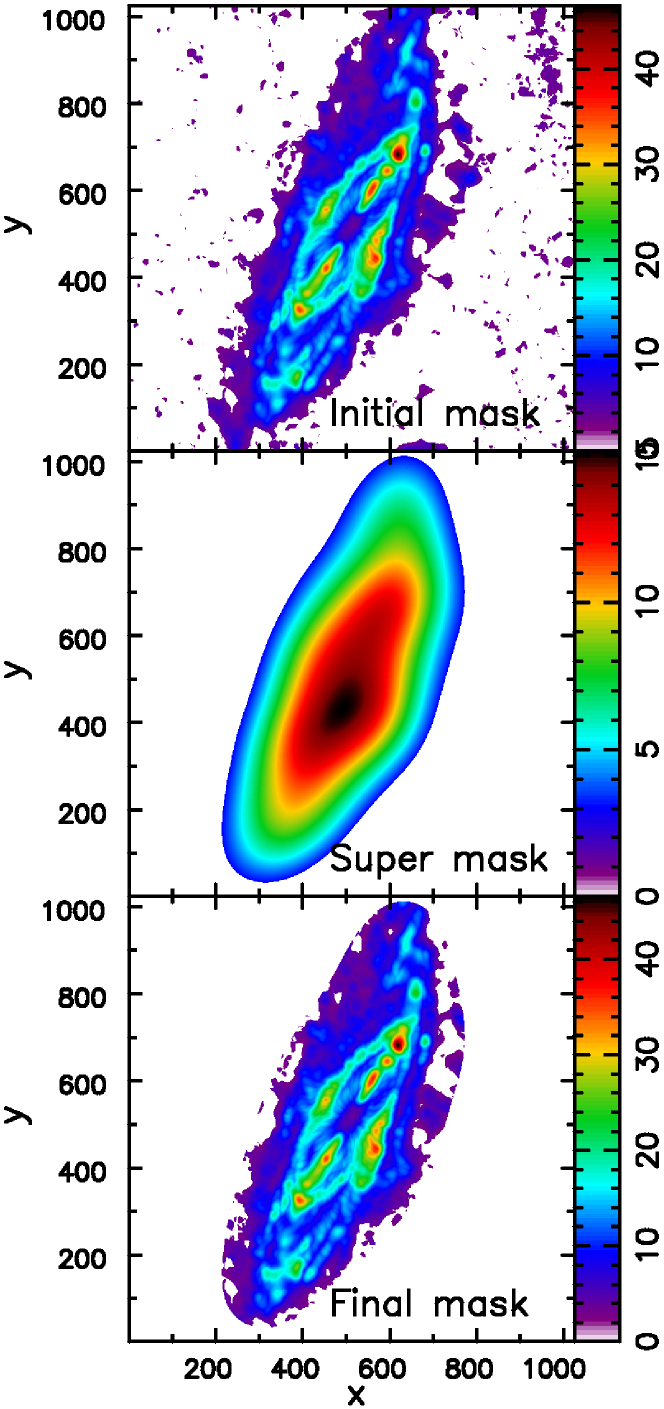
Figure 4: Illustration of our procedure to make the mask using the natural weights THINGS data cube for NGC 2841. The colored pixels in the top panel indicate the peak intensity, in units of ${\cal N}_{s}$, in the data cube smoothed by $30\arcsec$, while the white pixels are those below the threshold described in the text. The middle panel is the result of heavily smoothing the image in the top panel and clipping away values below $3{\cal N}_{s}$, which we describe as the super mask. The final map in bottom panel is the result of masking the top panel with the non-zero values in the super mask. The final mask we employ selects only those pixels that have non-zero values in this last map.

Following Walter et al. (2008), we begin by smoothing the emission in each channel map by convolving with a Gaussian of FWHM 30″. (Since the beam size in THINGS observations is already typically 10″, the resulting resolution of the smoothed data is $\sim 32$″.) We then calculate the global level of noise in the smoothed map, ${\cal N}_{s}$, again as the bi-weight estimate of a Gaussian spread of the intensity in the outermost two planes of all six faces of the smoothed data cube. Then working over all $(x,y)$ pixels in turn, we consider the pixel to have real emission if the smoothed intensity in three consecutive velocity channels is greater than $2{\cal N}_{s}$, as recommended by Walter et al. (2008). The color scale in the top panel of Figure 4 shows the peak intensity, in units of ${\cal N}_{s}$, in every pixel of the smoothed cube that is accepted by this criterion. The area containing the emission from the galaxy stands out, but we need to do more to discard the many pixels away from the galaxy that are also above the threshold. The final masks created by Walter et al. (2008) also resulted from additional steps, that were not described in their paper (de Blok 2020, private communication).

We therefore smooth the map in the top panel using a much broader kernel of FWHM $\sim 71$ pixels, or $106\arcsec$ for this image, obtaining the “super mask” map shown in the middle panel of Figure 4. Here we have clipped away all pixels for which this heavily smoothed intensity is $<3{\cal N}_{s}$ in all velocity channels. We could use the non-blanked channels of this super mask as our mask, but we prefer to mask out any pixels within this area that were previously masked in the top map, but have been resurrected by smoothing. This procedure leads to the final map shown in the bottom panel. Our mask becomes a binary acceptance of any pixel that is colored in this map. It excludes all pixels that are well outside the galaxy, while generously including the entire area containing emission from the galaxy.

Note that we discard the smoothed data cube after the mask is determined, and follow standard practice to fit emission lines to the data in the original unsmoothed cube.

3.2 Extracting velocity and uncertainty maps

We have remade velocity maps by the method described in §2 from the standard data cubes of 18 of the 19 galaxies in the subsample of THINGS galaxies selected for rotation curve analysis by dB08. The one exception is M81 (NGC 3031), which had been observed in two separate VLA pointings and for which the available data cube is not in the standard form.

For each fitted galaxy, the Appendix presents the resulting velocity maps and maps of the velocity uncertainties for each case. Our standard set of parameters for makemap is: $I_{n,\rm min}=0.5$, $A_{\rm min}=2$, $h_{3}$ included but $h_{4}$ excluded, $w_{\rm max}=50\delta v$, $h_{\rm max}=5$, and $n_{\rm boot}=20$.

3.3 Extracting rotation curves

The DiskFit package differs fundamentally from rotcur in that it tries to fit a single idealized global model for the galaxy to the entire observed velocity map. In its simplest form, the model is a flat, inclined disc in which the gas flows on circular orbits at speeds that are tabulated at finite set of radii. Such a model has five global parameters, the systemic velocity of the galaxy, $V_{\rm sys}$, the position of the centre of rotation $(x_{\rm cen},y_{\rm cen})$, the inclination, $i$, of the disc to the line of sight, and the position angle, PA, of the major axis of the projected disc to due north. DiskFit can also allow that the flow in part of the disc is intrinsically non-circular in a bar-like or oval distortion in the same plane as the overall disc, or that the disc is intrinsically warped in a simple parameterized manner.

DiskFit proceeds by adjusting the parameters of the global fit to find those that minimimize

$$\chi^{2}=\sum_{\rm pixels}\left[{V_{\rm line}-V_{\rm model}\over\sigma}\right]^{2},$$ (3)

where $V_{\rm line}$ is the estimated velocity from the Doppler shift of the line at each pixel and $\sigma$ is the adopted uncertainty in $V_{\rm line}$. The predicted velocity at each pixel, $V_{\rm model}$, is computed by interpolation between a set of ellipses at which the circular speed, and any non-circular streaming motions, are tabulated. For each set of global parameters, the optimal choices for these velocities is first determined by matrix inversion (see Spekkens & Sellwood, 2007, for details).

Our line fitting procedure (makemap, §2) returns an estimate of the uncertainty, $\sigma_{\rm line}$, in the fitted velocity at each pixel that, if used as the denominator in eq. (3), would have the desirable effect of giving high relative weight to pixels with small velocity uncertainties. Since the median uncertainty in the fitted velocity is typically $<3\;$km s^-1, and some are a small fraction of this, the pixels having the smallest values of $\sigma_{\rm line}$ would dominate the global fit to an excessive extent, however. We think it unlikely that the line-of-sight velocity at a particular location can be determined with a precision that is a small fraction of the level of turbulence in the ISM within a galaxy. We therefore choose a non-zero value for $\Delta_{\rm ISM}$, which is a global constant that we add in quadrature to the values of $\sigma_{\rm line}$ at each pixel and set $\sigma=(\sigma_{\rm line}^{2}+\Delta_{\rm ISM}^{2})^{1/2}$ in eq. (3). The larger the value of $\Delta_{\rm ISM}$ the less strongly the pixels are weighted towards those where the velocity is well determined.

It is important to note that not only have we propagated the uncertainty in the fitted velocity in each pixel into the global minimization, but DiskFit returns uncertainties in all the fitted global parameters and estimated orbit speeds at each radius that are determined by a modified bootstrap method proposed by Sellwood & Zánmar Sánchez (2010). Their method assumes that we see the galaxy as a disc in projection and attempts to preserve coherent line-of-sight velocity residuals arising from spiral-arm streaming. The algorithm deprojects the residual pattern to face on, rotates it through a random angle, and rescales it in radius before reprojecting, and then adds the resulting new residual pattern to the best fit model to create a pseudo data set for a new fit. For fits that include a bar flow, or oval distortion, we adopt the same procedure separately for the regions within the bar and outside it. This approach allows the user to estimate uncertainties in all the global parameters and the circular speed at each radius that not only take account of statistical errors from the observations, but also allows for spiral arm streaming, turbulence and other possible departures of the galaxy from the simple model adopted. Furthermore, we examine the spreads in the values of global parameters for possible covariances that may indicate inadequacies in our model.

These capabilities contrast strongly with the tilted-ring approach used in rotcur, which is widely employed and was adopted by dB08, in particular. To wit: DiskFit assumes a generally flat disc, with a fixed $V_{\rm sys}$, centre, PA, and $i$ for the whole galaxy, whereas all these quantities can optionally be allowed to vary from ring to ring in rotcur. Furthermore, uncertainties in the circular speed generally quoted by users of rotcur are estimated separately for each ring and take no account of uncertainties in the systemic velocity, projection geometry, or global inadequacies of the tilted-ring model.

In the present application to the THINGS data, we discard pixels for which the fitted line is flagged as bimodal, and estimate uncertainties from 200 bootstrap iterations. We have adopted values in the range $1\leq\Delta_{\rm ISM}\leq 8\;$km s^-1, choosing smaller values generally for dwarf galaxies. Small changes to $\Delta_{\rm ISM}$ have little effect on the fit, but we found it was sometimes necessary to employ larger values when $\chi^{2}$ became excessive. Although we do not attach any meaning to this statistic, and therefore do not quote it, values of $\chi^{2}\ga 5$ per degree of freedom were a warning that the fit was being driven by the pixels having small $\sigma$ in equation (3). Raising the value of $\Delta_{\rm ISM}$ in these cases naturally reduced $\chi^{2}$ and improved the behaviour of DiskFit.

As noted above, DiskFit tabulates the rotation curve at a set of radii, or more precisely ellipse semi-major axes, and the model predictions are interpolated between the tabulated ellipses for each pixel in equation (3). Thus the sampling of the rotation curve can be much coarser, typically 1 - 4 beam widths, in contrast to every half-beam width that is preferred in rotcur. The beam sizes in the individual THINGS galaxies are given in Table 3 of Walter et al. (2008), and the FWHM are in the range 5″to 15″.

Galaxy	$\Delta_{\rm ISM}$	$V_{\rm sys}$	$i$	PA	centre RA	centre $\delta$	bar PA in
name	km s-1	km s-1	deg	deg	pixels	pixels	disc plane: deg
NGC 925	5	$548.7\pm 3.0$	$61.5\pm 2.8$	$-75.7\pm 1.0$	$518.5\pm 5.2$	$516.9\pm 4.2$
NGC 2403	8	$132.8\pm 1.1$	$61.8\pm 1.7$	$124.1\pm 0.5$	$1020.8\pm 4.0$	$1008.9\pm 2.9$
NGC 2841	5	$631.0\pm 1.9$	$73.7\pm 1.3$	$148.6\pm 1.5$	$508.1\pm 1.0$	$513.2\pm 1.5$
NGC 2903	8	$552.9\pm 1.1$	$64.4\pm 0.9$	$203.1\pm 0.8$	$510.7\pm 0.6$	$513.8\pm 1.4$	$230.6\pm 11.4$
NGC 2976	5	$3.2\pm 0.8$	$58.4\pm 0.8$	$-36.5\pm 0.3$	$514.5\pm 1.2$	$515.8\pm 1.1$	$155.6\pm 4.9$
IC 2574	5	$45.4\pm 4.3$	$47.7\pm 9.9$	$57.2\pm 1.7$	$544.2\pm 26.6$	$524.1\pm 17.4$
NGC 3198	5	$683.9\pm 0.7$	$71.1\pm 0.8$	$215.6\pm 0.5$	$511.4\pm 0.8$	$512.9\pm 1.0$
NGC 3521	8	$789.4\pm 4.2$	$70.9\pm 1.2$	$-20.0\pm 0.7$	$506.2\pm 1.8$	$513.8\pm 2.8$
NGC 3621	8	$727.4\pm 1.2$	$64.7\pm 0.9$	$-15.9\pm 0.4$	$507.8\pm 1.5$	$511.2\pm 1.8$
NGC 3627	8	$710.7\pm 2.8$	$56.7\pm 2.4$	$172.9\pm 2.1$	$508.9\pm 1.7$	$513.8\pm 1.9$	$60.2\pm 14.9$
NGC 4736	8	$310.1\pm 0.5$	$31.7\pm 5.1$	$-55.1\pm 1.1$	$512.6\pm 0.5$	$513.4\pm 0.4$	$241.9\pm 7.7$
DDO 154	1	$375.1\pm 0.4$	$64.1\pm 1.3$	$225.6\pm 0.5$	$503.2\pm 1.5$	$510.5\pm 1.7$
NGC 4826	8	$411.1\pm 1.7$	$64.3\pm 2.0$	$122.1\pm 2.0$	$514.5\pm 0.8$	$517.1\pm 0.9$
NGC 5055	5	$502.0\pm 1.4$	$65.8\pm 0.6$	$100.2\pm 0.6$	$516.1\pm 1.0$	$513.2\pm 0.4$
NGC 6946	6	$51.0\pm 2.1$	$36.4\pm 3.8$	$243.0\pm 1.0$	$513.6\pm 5.3$	$517.9\pm 5.5$
NGC 7331	8	$816.4\pm 4.0$	$76.0\pm 0.8$	$169.9\pm 0.5$	$511.8\pm 0.6$	$513.7\pm 1.9$
NGC 7793	4	$228.4\pm 0.3$	$43.9\pm 4.3$	$-65.0\pm 0.9$	$506.1\pm 0.7$	$516.6\pm 1.2$	$50.8\pm 5.3$

Table 1: The 17 galaxies in our sample and parameters of the best fit models in each case obtained by applying DiskFit to our re-derived velocity map. The values of $V_{\rm sys}$, $i$, and PA may be compared with average values given in Table 2 of de Blok et al. (2008), who employed rotcur to fit tilted ring models to their own velocity maps derived from the same data cubes.

4 Results

Of the 18 THINGS galaxies for which we made new velocity maps, we fitted rotation curves using DiskFit to 17; fits to the remaining galaxy, NGC 2366, were not believable (see §4.3.3). The rotation curves from DiskFit are also presented in the Appendix, together with maps of residuals after subtracting the best fit model, and notes on the individual galaxies. Table 1 gives the global parameters of the fitted models, and their uncertainties, as well as the adopted value of $\Delta_{\rm ISM}$ in each case.

Our fitted rotation curves are generally, with 2 or 3 exceptions, in good agreement with those already published by dB08 who derived their velocity maps independently and employed rotcur to estimate the circular speed at each radius. However, our estimates of the uncertainty in the circular speed generally differ from theirs. The rotation curves reported in the later study by Ponomareva et al. (2016) that included many of the same galaxies were also generally similar, but these authors did not present uncertainties in the orbit speeds at each radius. Sellwood & Zánmar Sánchez (2010) had previously used an earlier version DiskFit to extract rotation curves for five THINGS galaxies. Since we here rederive velocity maps using a different algorithm, we include these five galaxies in the present study.

We have employed a flat disc model in every case except NGC 2841, for which we fitted a mild, parametric warp, and NGC 5055. It is well known that warps are common in the outer discs of many galaxies; see Sellwood (2013) for a review of both the observational evidence and theory. The first of the three summary rules for warps deduced from observational data by Briggs (1990) is that the warp generally starts at $R_{25}$, the radius at which disc surface brightness in the blue band falls below 25 mag per square arcsec. This finding is in agreement with theory (e.g. Shen & Sellwood, 2006), which also predicts that the disc within $\sim 4$ disc scale lengths is expected to be rigid enough to stay flat.

However, an axisymmetric flat disc model was not a good fit to the part of the flow well within $R_{25}$ for five galaxies: NGC 2903, NGC 2976, NGC 3627, NGC 4376, and NGC 7793, which we therefore fitted with a bar or oval distortion. In these same cases, rotcur finds that the PA and/or inclination of the “disc” varies strongly in the region of the bar or oval flow, which is a natural consequence of insisting that an intrinsically elliptical flow pattern be modelled as motion in a circle. We are confident that such apparently pathological twists in the inner disc are an artifact of rotcur, and argue that the inner disc does in fact have a fixed projection geometry and instead gas is streaming in an elliptical flow pattern in a non-axisymmetric potential over part of the radial range.

Our fits to most galaxies do in fact extend well beyond $R_{25}$, yet we continue to find acceptable fits with a flat disc model, with little evidence in the velocity residuals for a warp, with the exceptions of NGC 2841 and NGC 5055 that we discuss below. The absence of a large warp in the outer disc is consistent with the findings of dB08 for which their fitted values of PA and/or $i$ generally vary by $\la 10^{\circ}$ from those in the inner disc. This statement remains true for the cases with bars when the region where we fit a bar is discounted, but does not hold for NGC 2841 and NGC 5055. Aside from these last two cases, we find that forcing a flat disc model does not lead to systematic discrepancies in the fitted circular speeds returned by DiskFit and rotcur.

Our fits to the velocity map of NGC 2841 were improved by allowing a mild parameterized warp model, as discussed in §4.3.2. The paramterization of the warp adopted in DiskFit was unsatisfactory for NGC 5055, however, and instead we found that an acceptable fit could be made by allowing separate fixed-projection geometries of the inner and outer parts of the disc, with the boundary at a semi-major axis of 375″, which is very close to the value $R_{25}=378$″ given in the RC3 (de Vaucouleurs et al., 1991). In fact, this can be achieved in a single fit without dividing the data by allowing for non-circular flows in the inner disc with the projected geometry set by the outer disc, as we report in the Appendix. Fitting the two parts of the flow with such a “bar model” is nothing more than a device to capture two flat, intrinsically circular flow patterns that are misaligned in the different parts of the galaxy. The values for the global parameters of NGC 5055 given in Table 1 are for the fit to the inner disc only, while the fitted values for the outer disc are $i=59.3\pm 1.1$ and PA$=92.7\pm 0.6$, with the centre held fixed at the same position as fitted for the inner disc.

4.1 Uncertainties in the fitted parameters

Uncertainites in the global parameters, as well as the circular speed at each radius, were estimated from 200 bootstrap iterations in DiskFit using in all cases the procedure recommended by Sellwood & Zánmar Sánchez (2010), as described above (§3.3).

We have not computed the covariance matrix, and instead present figures in the Appendix showing distributions of values of the fitted paramaters for each bootstrap iteration, with the best fit parameters marked in red. Our uncertainties in the parameters quoted in table 1 are computed from the spreads of these values in the coordinate directions. These figures are generally reassuring because the best fit model usually lies near the centres of these distributions and there are few pronounced correlations between the parameters. The most obvious exception is that the systemic velocity of some galaxies correlates with the fitted position of the centre along the major axis, especially for dwarf galaxies for which the rotation curve rises slowly. This is to be expected, since it is well-known that the velocity map of a hypothetical galaxy having an exactly linearly rising rotation curve cannot constrain either the position of the centre along the major axis, and consequently the systemic velocity, or the galaxy inclination (Bosma, 1978). All the THINGS galaxies rotate differentially to some degree, which breaks these exact degeneracies, but a vestige of them lingers in the parameter correlations from the bootstrap iterations, and is particularly pronounced for IC 2574 (Figure 12).

It should be noted that one of the reasons that we rejected all our attempts to fit a model to the data for NGC 2366 was that the “best fit” models were outliers in all the parameter covariance plots. Rearranging the large velocity residuals in this case seemed always to lead to fits for which the global parameters differed from the best fit values in a lop-sided sense. We interpreted this as a red flag to indicate that the best fit should not be accepted, as we note below in the discussion of this galaxy in §4.3.3. The ability to provide this kind of warning diagnostic to flag doubtful fits is unique to our analysis methods.

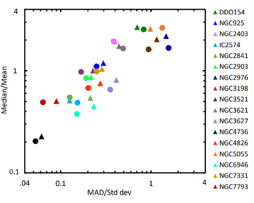
Figure 5: Comparison of velocity uncertainties from rotcur and DiskFit as described in the text. For each galaxy, we compute the ratio of the uncertainties from rotcur to those from DiskFit, and characterize the distribution of values in four ways. The circles mark the median as a function of median absolute deviation (MAD), while the triangles give the mean as a function of standard deviation. The data from the figures in de Blok et al. (2008) were kindly provided in digital form by Erwin de Blok.

4.2 Circular speed uncertainties

The figures in the Appendix present estimated circular speeds, as well as their uncertainties, as functions of radius both from our work (points with error bars) and those from dB08 (red lines with grey shading). Figure 5 summarizes how the two sets of uncertainty estimates compare. To make this Figure, we computed the ratio of the error estimates reported by dB08 divided by those given by DiskFit. Since dB08 sample the rotation curve more densely, we interpolate their error estimates to the radius of the DiskFit point, omitting values where the two RCs do not overlap and where we included a bar/oval. We then derive four measures of the distribution of ratios for each galaxy: the mean, standard deviation, median, and median absolute deviation (MAD), as shown in the Figure.

In some galaxies (e.g. IC 2574, NGC 4736, NGC 6946 and NGC 7793) our uncertainties are substantially larger than those reported by dB08, which is usually attributable to a significant uncertainty in the inclination of the disc to the line-of-sight, a source of uncertainty that rotcur ignores. In other cases (e.g. DDO 154 and NGC 5055), our uncertainties are substantially smaller than theirs. In the remaining cases there is approximate agreement, although in NGC 2841 and in NGC 3521 we disagree over just part of the radial range. Our substantially smaller uncertainties in the outer part of the rotation curve for NGC 3521 probably stem from our elimination of pixels for which the line profile was flagged as bimodal, as the data cube appears to include emission from a, possibly infalling, gas stream having a line-of-sight velocity below that of the circular speed in the disc mid-plane.

4.3 Three examples

Here we highlight our findings for three galaxies that illustrate the power of our methods.

4.3.1 DDO 154

This dwarf galaxy is extremely well fitted by our flat, axisymmetric disc model, since the velocity residuals, Figure 18, are generally small. The covariance plots in the bottom panel of the same figure reveal that each global parameter of the best fit model, red symbols, is near the centre of the distribution of values from the 200 bootstrap iterations, and the projection geometry is tightly constrained. Strong degeneracies between the location of the centre, the inclination, and systemic velocity can arise when fitting velocity maps of dwarf galaxies, but in this case they are mild, with just weak correlations in the expected sense between $V_{\rm sys}$ and the $(x,y)$ position of the centre. dB08 allow $i$ and PA to vary with radius, but remark that they ignore the variation near the centre and in the outer parts because both regions suffer from sparse data, and extrapolate from the almost constant and better constrained values at intermediate radii. Their table 2 gives $V_{\rm sys}=375.9\;$km s^-1, and average values of $i=66.0^{\circ}$ and PA$=229.7^{\circ}$, in good agreement with our values in Table 1. Our rotation curve agrees well with that of dB08, but our estimated uncertainties in the circular speed are substantially smaller than theirs.

In summary, our work strengthens the evidence from previous studies that this galaxy has a particularly well-determined rotation curve with very little wiggle room for comparisons with predictions.

4.3.2 NGC 2841

As fits to the velocity map of this galaxy were unsatisfactory when DiskFit assumed a flat disc, we allowed for a gradual mild warp. The parameterized warp fitted by DiskFit allows for a change of both inclination and position angle with radius that varies in a quadratic fashion from zero change at the inner radius $R_{\rm warp}$ to a maximum at the edge. Thus there are three additional global parameters to be fitted: the radius at which the warp starts, $R_{\rm warp}$, and the maximum changes in ellipticity $w_{\epsilon,\rm max}$ and PA $w_{\phi,\rm max}$.

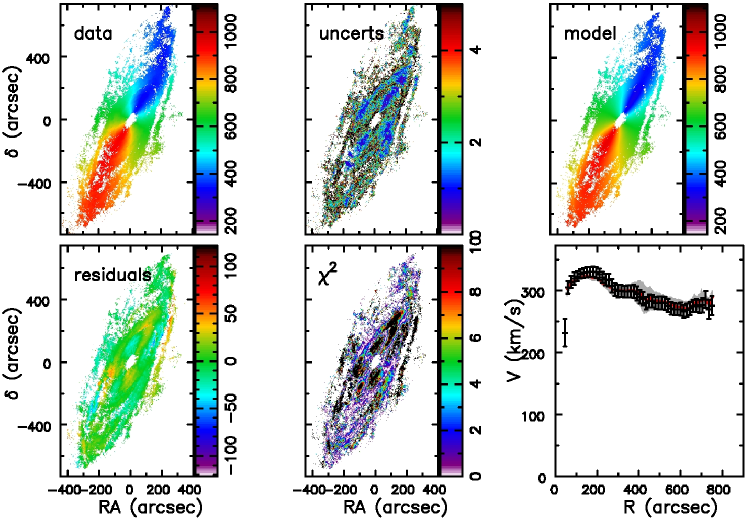
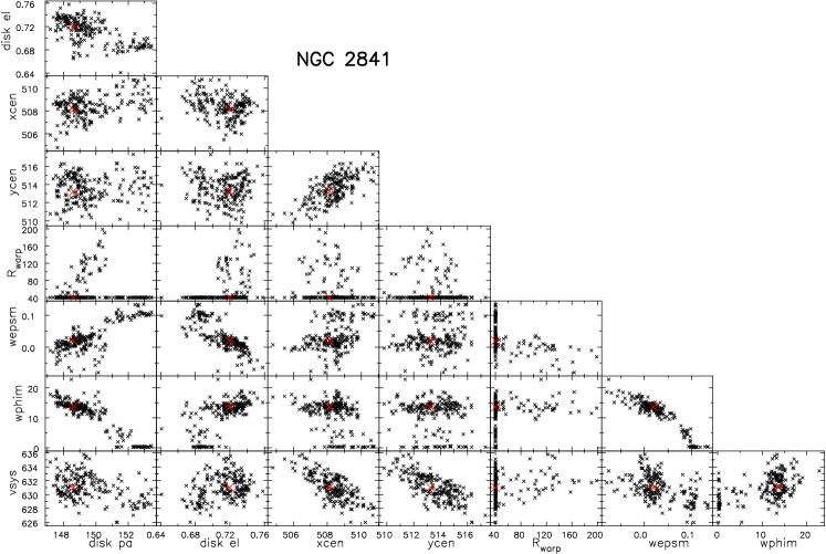
Figure 9: As in Figure 7, but for NGC 2841.

The results are displayed in Figure 9. The covariance plots are generally well behaved, but many values of $R_{\rm warp}$ are clustered at the low end of the range, because we created a wall in the $\chi^{2}$ function to prevent $R_{\rm warp}$ from straying below the radius of the second fitting ellipse. The other parameters of the mild warp are: $w_{\epsilon,\rm max}=0.02\pm 0.04$, which corresponds to an increase in inclination of $\sim 3^{\circ}$ from the centre to the edge, while the PA of the major axis increases from the centre to the edge by $w_{\phi,\rm max}=13.6^{\circ}\pm 2.4^{\circ}$.

Table 2 of dB08 gives $V_{\rm sys}=633.7\;$km s^-1, and average values of $i=73.7^{\circ}$ and PA$=152.6^{\circ}$. The angles in our Table 1 apply to the inner disc. The change in PA that we fit is about the same as that reported by dB08, but those authors report an increase in $i$ of some 8^∘, which is larger than we find.

Our rotation curve is in excellent agreement with the fit reported by dB08 and our uncertainties are similar to their estimates in the outer disc and a little larger than theirs in the inner disc.

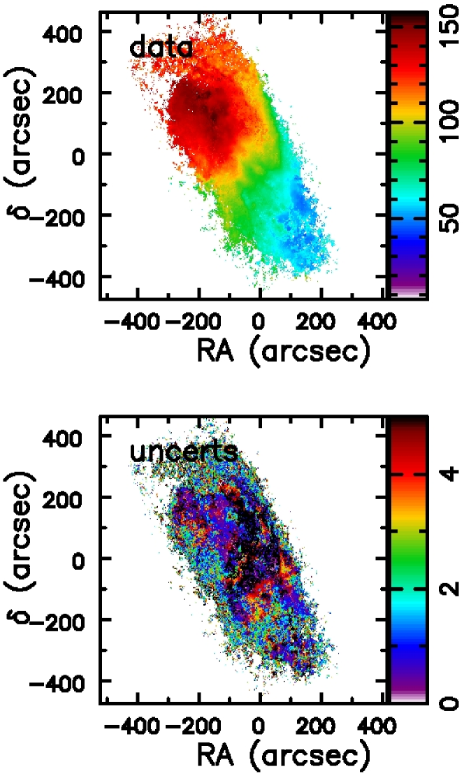
Figure 6: Our velocity map (above) with uncertainties (below) for NGC 2366.

4.3.3 NGC 2366

We were unable to find a credible model that fitted the velocity map of the dwarf galaxy NGC 2366. The upper panel of Figure 6 manifests a clear velocity gradient roughly aligned with the major axis of the HI emission, but the iso-velocity contours do not appear to have the characteristic pattern of flow in flat, axisymmetric disc. Note also in the lower panel that many pixels near the centre of our velocity map have uncertainties $>5\;$km s^-1.

The rotation curve reported by dB08 rises to nearly 60 km s^-1 around 250″, but then drops below 40 km s^-1 by 420″, which is a steeper than Keplerian fall off. Similar shapes were also reported in previous studies (Swaters, 1999; Hunter et al., 2001). Oh et al. (2008), on the other hand, obtained a quite different fit to the same data cube, which is also reported in dB08. They suggested the circular speed continues to rise for $R>300\arcsec$, finding an essentially flat, axisymmetric disc in the outer parts. They obtained this result by applying rotcur to a map of the “bulk velocity” in the line profiles as described in their paper.

Our attempts to use DiskFit to fit a flat, axisymmetric model to our full map yielded a bizarre rotation curve, which was scarcely improved by allowing an oval distortion. A strongly warped disc model yielded a better fit with a more reasonable rotation curve, but with large and coherent residuals. However, the rotation centre was far from the centre of the map, and the deprojected data filled only slightly more than a semi-circle. This circumstance precluded the use of the bootstrap method proposed by Sellwood & Zánmar Sánchez (2010), which assumes a round disc seen in projection in which spiral streaming motions are the main failing of the model. We were therefore forced to use the earlier bootstrap method proposed by Spekkens & Sellwood (2007) that attempted to preserve the patchwise coherence of the velocity residuals. This method left the “best fit” model as an outlier from the cluster of values in the covariance plots in most parameters, which is another red flag, and we therefore doubted this fit also.

Furthermore, discarding some of the data in the outer parts of the map caused substantial changes to the fitted position of the centre, the overall inclination, the magnitude of the warp, and the estimated rotation curve. We were unable to find a significant subset of the data that would yield consistent values for any of these parameters.

We therefore conclude that the gas in this dwarf galaxy does not follow a simple flow pattern in even a twisted disc and do not present a fitted model for this galaxy.

5 Discussion and conclusions

Any meaningful comparison between a model prediction and observations requires that the data with which the model is compared have well-defined uncertainties so that the likelihood that the model matches the data can be assessed. In the case of rotation curves derived from high resolution 21cm line observations of nearby galaxies, the uncertainties in the fitted circular speed have not, as yet, been derived in a statistically meaningful manner, and therefore the success of galaxy formation models in predicting the observed data cannot be quantified.

As a further step towards the goal of a meaningful comparison, we have presented a new standalone tool, makemap, to extract 2D velocity maps from 3D data cubes of spectral line data. Unlike previous approaches to extract velocity maps from high resolution spectral data cubes, our method estimates the uncertainty in the fitted velocity in each pixel that takes into account the clumpy and turbulent nature of the ISM in the observed galaxy. The estimated velocity uncertainties can then be propagated into the procedure to fit a model to the velocity map. The modern methods we reviewed in the introduction that attempt to fit a model directly to the 3D data cube, without the intermediate step of making a velocity map, are inefficient when applied to high spatial resolution data, and also have not, thus far, attempted to estimate uncertainties in a well-founded manner.

From previous work (Spekkens & Sellwood, 2007; Sellwood & Zánmar Sánchez, 2010), we have made public a model fitting program, DiskFit, that is an improvement over the usual tilted-ring fitting procedure to extract rotation curves because it estimates uncertainties in the fitted circular speed that take account of large-scale turbulence, spiral arm streaming motions, as well as global uncertainties in the position of the centre, the systemic velocity, and the inclination and position angle of the galaxy to the line of sight. In the absence of uncertainties in the observed velocities to be fitted by the model, this code simply assumed a constant uncertainty in the fitted velocity in each pixel in the map. But our new map making tool provides uncertainties in the fitted velocity at each pixel that can now be propagated into the model fitting.

Here we have applied both the new tool, makemap, together with DiskFit to the publicly available data cubes of 17 galaxies from the THINGS survey (Walter et al., 2008). Our re-analysis these data has generally confirmed the rotation curves derived by de Blok et al. (2008), although we find a few differences. We have adopted flat disc models for most of the galaxies, allowing a bar-like or oval distortion in the inner parts of five galaxies, whereas the tilted ring analysis by dB08 generally fitted the same data with strong twists to the disc plane. Our model for NGC 2841 included a mild warp, consistent with the findings of dB08. The velocity map of NGC 5055 is also consistent with an abrupt warp that begins near $R_{25}$, and we have fitted this galaxy with separate inner and outer flat discs having different projection geometries.

More importantly, we believe our analysis provides better-founded uncertainty estimates that reflect both the uncertainties in the data and in the projection parameters as well as non-circular streaming motions. In this sense, we have taken a step towards the ultimate goal of statistically valid uncertainties. We do claim that our quoted uncertainties in model parameters and rotation curves are more reasonable than those in previous work, but do not claim to have evaluated them with full statistical rigour. Our uncertainties are sometimes a few times greater than those given by dB08, and sometimes just a fraction of their values.

We highlight two example galaxies from our study to illustrate which nearby galaxies provide useful comparisons with model predictions, and which do not. We find that the data on DDO 154 are extremely well fitted by a simple, flat axisymmetric flow pattern having tightly constrained projection parameters and that dB08 in fact overestimated the uncertainties in the fitted circular speed. On the other hand, we could not find a credible fit to the data from NGC 2366. Therefore we would argue that DDO 154 provides an excellent test case for comparison with galaxy formation models, but that nothing useful could be learned from including NGC 2366 in such a study.

dB08 fitted mass models to their rotation curves, weighting each data point by the inverse square of their estimate of its error. A similar fitting procedure to our very similar derived rotation curves would, to be sure, be differently affected by our different uncertainties, perhaps leading to slightly different best fit models. However, our key point is that having more realistic uncertainties would enable us to assess the likelihood that the data matches any fitted model, something that no previous study that we are aware of has attempted to quantify. We therefore defer this major task to a separate paper.

Data availability

The tools makemap and setmask will be added to the DiskFit package website: https://www.physics.queensu.ca/Astro/people/KristineaSpekkens/diskfit/. The raw data cubes are avaliable on the THINGS website (https://www2.mpia-hd.mpg.de/THINGS/Data.html). Our maps, models, rotation curves and uncertainties are available on request.

Appendix A Fits to individual galaxies

Here we present new velocity maps, with uncertainties, created by makemap for 17 THINGS galaxies, together with model and residual maps and rotation curves fitted to the new velocity maps using DiskFit. The best fit global parameters are given in Table 1, and the uncertainties and error bars on the fitted circular speeds are derived from 200 bootstrap iterations. For each galaxy, we also present plots to test for covariances between the fitted global parameters and provide a short narrative discussion of each case.

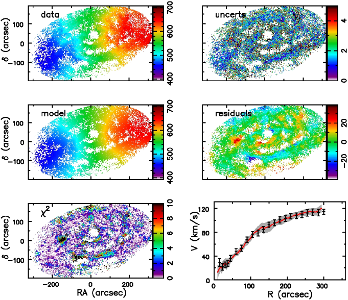
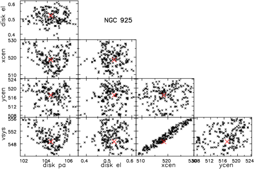
Figure 7: NGC 925 Top left: the velocity map extracted from the THINGS “standard cube”, with line-of-sight velocity in km s^-1 colour coded as indicated, and top right the uncertainty in the fitted velocity, also in km s^-1. 2nd row left: the best-fit model from DiskFit, and right the map of residual velocities after subtracting the fitted model from the data. Third row left, map of the values of $[(V_{\rm line}-V_{\rm model})/\sigma]^{2}$. Third row right: the black points with error bars show the fitted rotation curve, with the error bars resulting from 200 bootstrap iterations. The bottom panel shows the covariance of the global parameters; $V_{\rm sys}$ strongly correlates with $x_{\rm cen}$ because the major axis is close to the $x$-axis. The best fit projection parameters with uncertainties are given in Table 1. The red line in the rotation curve panel is that presented in dB08 with their estimates of the uncertainties indicated by the shading.

A.1 NGC 925

This dwarf galaxy has a simple velocity map that is reasonably well fitted as an axisymmetric, inclined disc. The black points with error bars in the third row right panel of Figure 7 indicate our fitted rotation curve and its uncertainties, which are in reasonable agreement with the same quantities estimated by dB08, marked by the red line and grey shading. The kink in the red line occurs at the radius where their rotcur analysis finds a discontinuity in the disc inclination, which we do not reproduce in our flat disc fit. The residuals map has few large values but does not reveal any tell-tale coherent features that would suggest a non-axisymmetric potential. We conclude that our axisymmetric model is a reasonable, albeit imperfect, fit to the data.

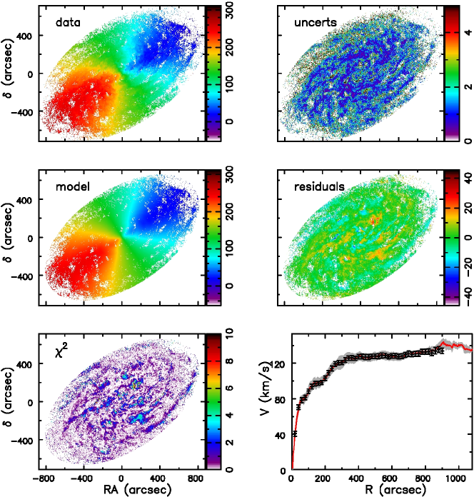
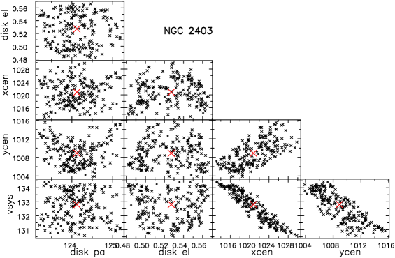
Figure 8: As in Figure 7, but for NGC 2403.

A.2 NGC 2403

Our flat, axisymmetric disc model fits the data from this galaxy very well, as shown in Figure 8. The rotation curve is in excellent agreement with that from dB08, and also Sellwood & Zánmar Sánchez (2010), although our uncertainties tend to be smaller than those quoted by the THINGS team. Sellwood & Zánmar Sánchez (2010) were unable to find evidence for a significant non-axisymmetric component in the potential. Our fit excluded gas emission beyond 900″ because at least some of it caused the rotation curve to drop at those radii. We suspect that this behaviour was due to gas at anomalous velocities that was not eliminated by our mask.

A.3 NGC 2841

As fits to the velocity map of this galaxy were unsatisfactory when DiskFit assumed a flat disc, we allowed for a gradual mild warp, as described in §4.3.2.

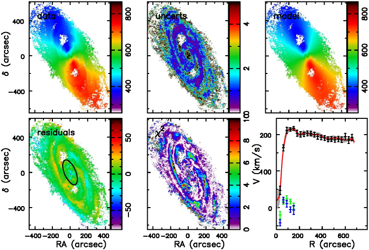
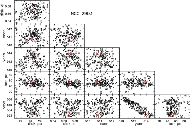
Figure 10: As in Figure 7, but for NGC 2903. The green and blue points with error bars indicate the fitted radial and azimuthal velocity components of the bar flow, which is fitted inside the ellipse drawn on the residuals map.

A.4 NGC 2903

Since the $3.6\,\mu$m Spitzer image shows the disc of this galaxy to be barred, we have included a bar flow to the fitted model in the inner part of the disc. The fitted radial and azimuthal bar flow velocities (Spekkens & Sellwood, 2007) are indicated, respectively, by the green and blue points with error bars. The bar flow velocities are small compared with the mean orbital speed, which agrees well with that estimated by dB08 who found, not surprisingly, that axisymmetric fits in the bar region required the PA and inclination to vary.

Sellwood & Zánmar Sánchez (2010) also used an earlier version of DiskFit and included a bar flow but to 60″ only. We find similar results as they did when we limit the non-asisymmetric part to the same region, but here allow for a somewhat more extensive bar flow. Even so, the residual velocity map manifests a coherent anti-symmetric ring, which is at a similar location as a ring in the HI column density and may possibly have some small radial velocity.

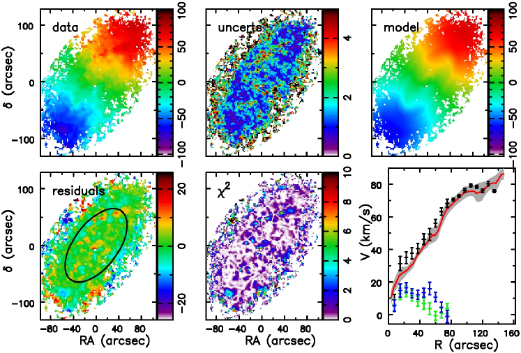
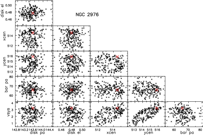
Figure 11: As in Figure 10, but for NGC 2976.

A.5 NGC 2976

Spekkens & Sellwood (2007) first showed that other velocity maps for this galaxy were better fitted with a bar flow, and this remains true for the THINGS data. As in our earlier work, and in Sellwood & Zánmar Sánchez (2010), fitting for an inner oval leads to higher estimated mean speeds over the radial range of the oval than were estimated by dB08. The THINGS team again reported large apparent changes in the fitted projection geometry that were caused by adopting an axisymmetric flow pattern where the flow is better fitted by oval streamlines in a flat disc.

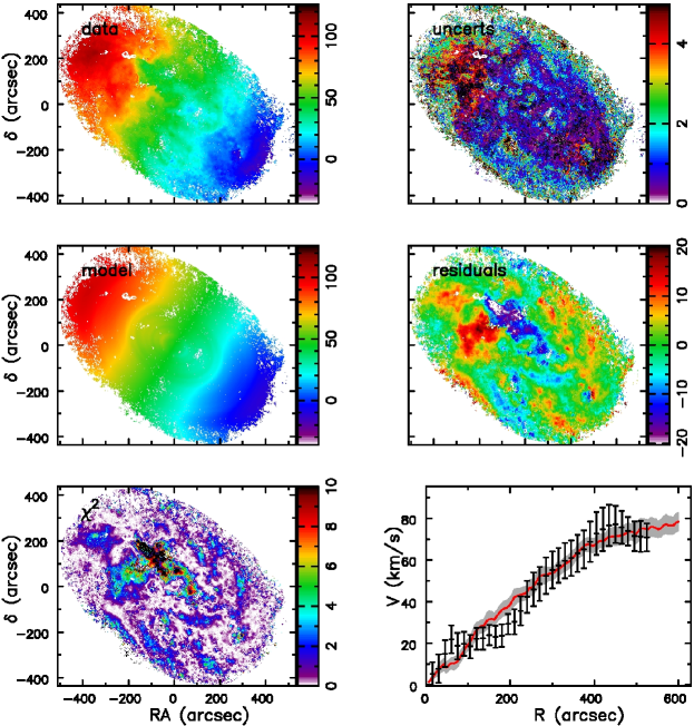
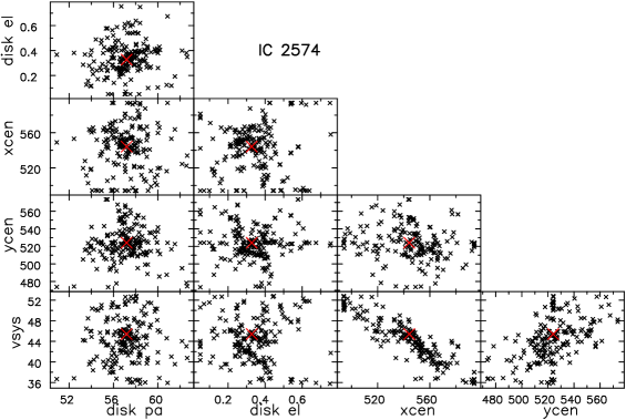
Figure 12: As in Figure 7, but for IC 2574.

A.6 IC 2574

This galaxy is a member of the M81 group and is surrounded by a number of substantial HI clouds Sorgho et al. (2020). It is not well fitted by our axisymmetric model Figure 12. Some of the velocity residuals are large, but there is no tell-tale pattern in them to suggest a non-axisymmetry in the flow and allowing a bar/oval component to the flow made only a marginal improvement. Our best fit inclination and systemic velocity (Table 1) are in good agreement with the values obtained by Sorgho et al. (2020) from their direct fits to their low resolution 3D data cube, but both differ significantly from the values given in table 2 of dB08, which are $i=53.3^{\circ}$ and $53.1\;$km s^-1. Also our rotation curve is in rough agreement with that reported by dB08 and better agreement with that derived from the lower resolution data by Sorgho et al. (2020). Our estimates of the uncertainties, which largely stem from an almost 10^∘ uncertainty in the fitted inclination (Table 1), are much greater than those suggested by the THINGS team.

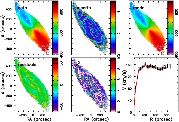
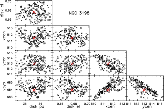
Figure 13: As in Figure 7, but for NGC 3198.

A.7 NGC 3198

A flat axisymmetric model fits the data from this galaxy very well, as is evident from Figure 13. Our fitted rotation curve and uncertainties are in good agreement with those estimated by dB08. Sellwood & Zánmar Sánchez (2010), who used an earlier version of DiskFit to search for non-axisymmetic distortions, failed to find any evidence for a distortion in the mid-plane potential of this well-studied galaxy.

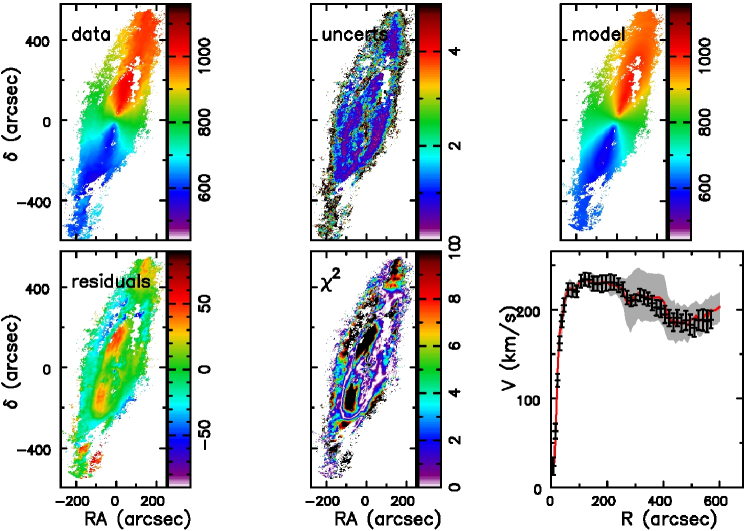
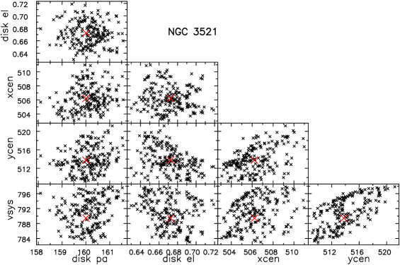
Figure 14: As in Figure 7, but for NGC 3521.

A.8 NGC 3521

Large parts of the velocity map of this galaxy have bimodal line profiles, possibly suggesting that emission is both from the disc and a stream of extra-planar gas. We have excluded pixels having bimodal line profiles and fit an axisymmetric model that has a declining rotation curve. Our fit, Figure 14, is in reasonable agreement with that from dB08, but our uncertainties are smaller, probably because we excluded pixels having bimodal profiles. The axisymmetric fit is hardly satisfactory because the velocity difference maps reveal areas of large coherent residuals, although we were unable to discern a coherent pattern to them.

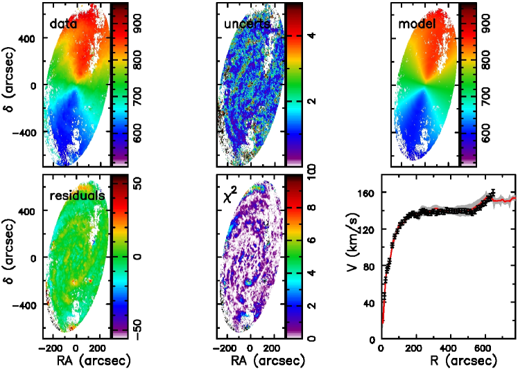
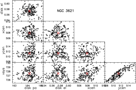
Figure 15: As in Figure 7, but for NGC 3621.

A.9 NGC 3621

This galaxy is well fitted by a simple axisymmetric disc flow model, as shown in Figure 15. The rotation curve agrees well with that given by dB08, although our uncertainties are smaller. Note that we masked away emission from gas outside the elliptical region shown, which appeared to have velocities that did not fit so well with our flat axisymmetric model. It is possible that a more sophisticated masking algorithm, that excludes gas having anomalous velocities, would allow our model to be extended to larger radii.

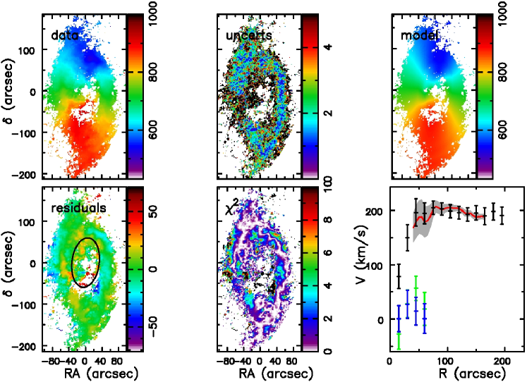
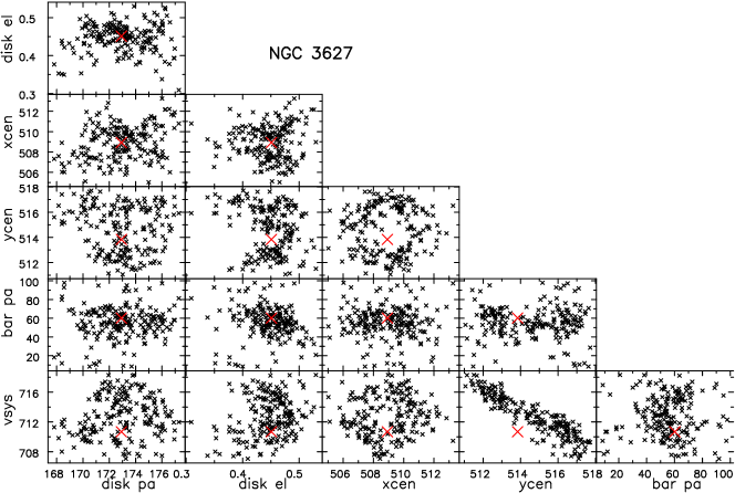
Figure 16: As in Figure 10, but for NGC 3627.

A.10 NGC 3627

As this galaxy is strongly barred, we have included a bar flow in the inner part of our fitted model, even though that part of velocity map is rather sparsely sampled. The resulting rotation curve is shown in Figure 16, with the fitted radial and azimuthal bar flow velocities (Spekkens & Sellwood, 2007) indicated, respectively, by the green and blue points with error bars. dB08 did not attempt to fit the barred region, but their outer rotation curve is in reasonable agreement with ours.

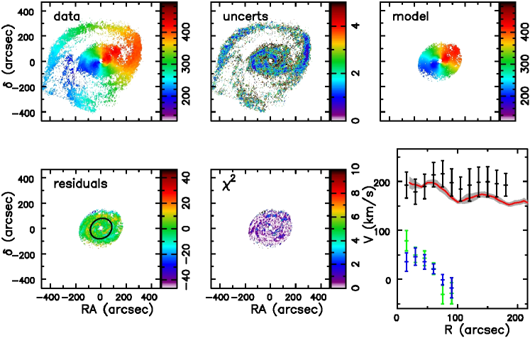
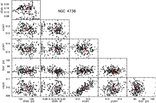
Figure 17: As in Figure 10, but for NGC 4736.

A.11 NGC 4736

As the outer parts of this galaxy appear to be tidally disturbed, we have fitted only the region inside $R=180$″. The resulting rotation curve is shown in Figure 17, with the fitted radial and azimuthal bar flow velocities (Spekkens & Sellwood, 2007) indicated, respectively, by the green and blue points with error bars. dB08 reported steep gradients in the apparent projection geometry within 100″, where we prefer a bar fit, and slightly more mild variations out to $R=400$″. Our model has generally higher orbit speeds than theirs over the radius range we fit. Our large uncertainties stem from the over 5^∘ uncertainty in the rather low inclination of the inner part of this galaxy. The covariance plots reflect the limit we impose that the disc ellipticity cannot fall below 0.05.

Our attempts to fit the outer parts of the map with an anti-symmetric warp model were unsuccessful, and we have concluded that the spiral feature encircling the north of the galaxy, together with the stream to the SE, are tidal debris that are either not in the main plane of the inner galaxy or not in circular motion, or both.

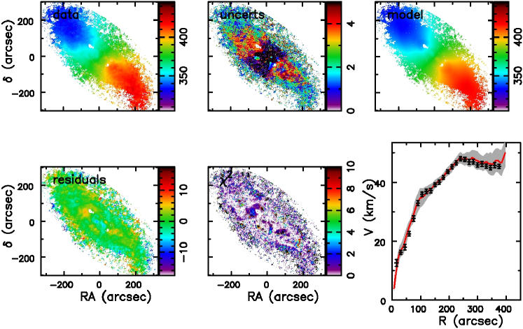
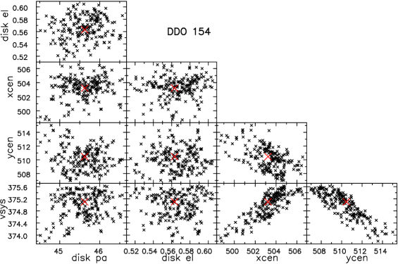
Figure 18: As in Figure 7, but for DDO 154.

A.12 DDO 154

This dwarf galaxy is extremely well fitted by a flat, axisymmetric disc model, since we estimate uncertainties in the circular speed (Figure 18) that are substantially smaller than those of dB08, but the rotation curves agree well. We discuss this result more fully in §4.3.1.

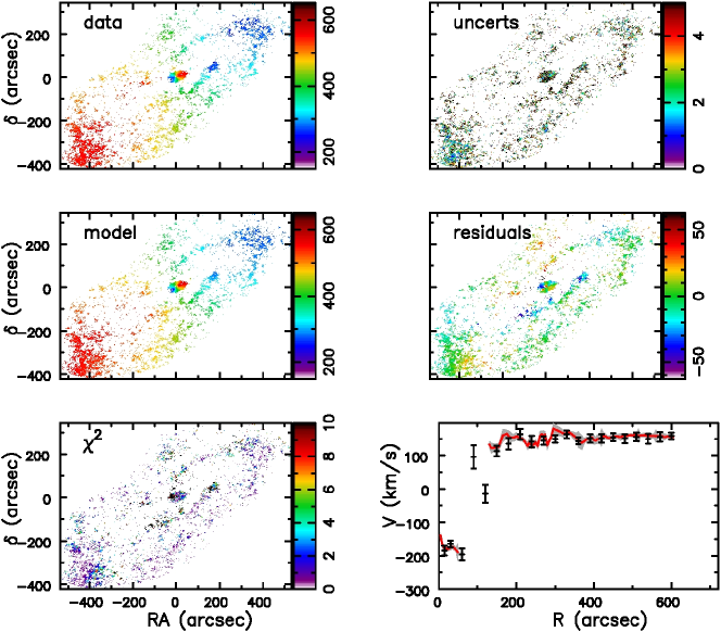
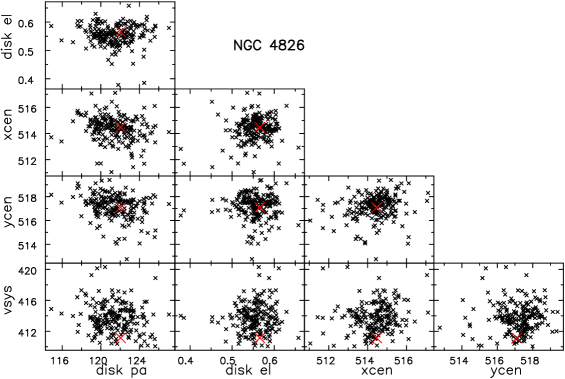
Figure 19: As in Figure 7, but for NGC 4826.

A.13 NGC 4826

The sparsely filled velocity map for this galaxy, Figure 19, can be fitted with an axisymmetric flat disc having a strongly counter-rotating core. These features are in good agreement with the fits reported by dB08, even though their fit suggests a substantial inclination change near the centre.

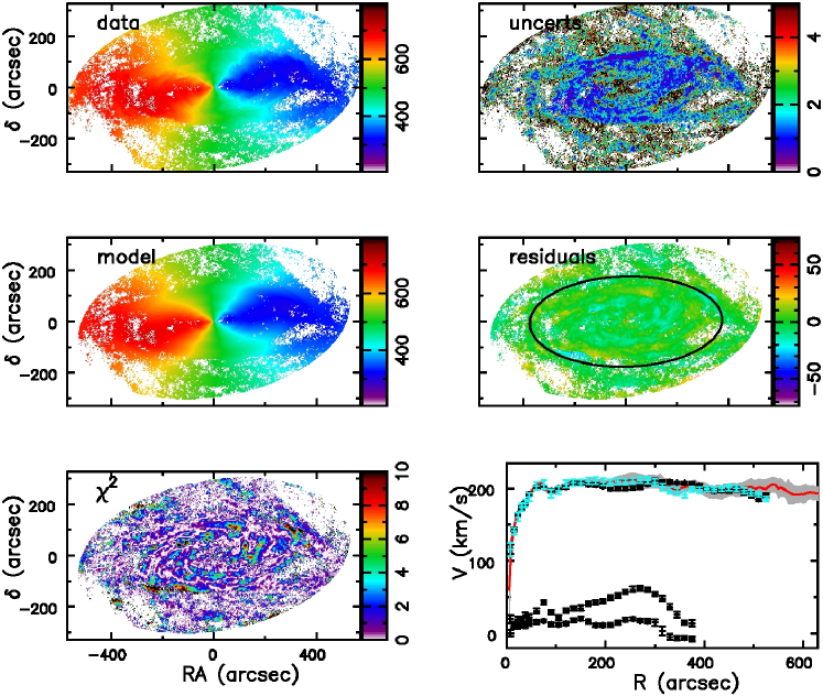
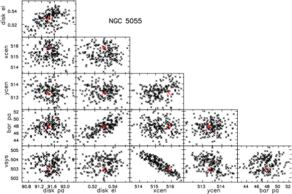
Figure 20: As in Figure 10, but for NGC 5055. In this case we have exploited the ability of DiskFit to fit two separately inclined parts of the disc in one fit (see the text for a fuller explanation). The small “non-circular” velocities of the inner disc returned by DiskFit are not physically meaningful. The cyan points indicate the fits to the separate inner and outer discs.

A.14 NGC 5055

As discussed in §4, a flat, axisymmetric disc model was not a good fit to the velocity map of this galaxy, and it seems that the HI layer beyond $R_{25}\simeq 378\arcsec$ lies in a different plane from that interior to this radius – i.e. the HI disc is warped. We have fitted the map inside and outside this radius with two separate flat discs and the fitted circular speeds of these two separate parts are marked in Figure 20 by the cyan points with error bars. The global parameters of the fit to the inner disc are given in Table 1 and those for the outer disc are reported in the text. The black points with error bars in Figure 20, many of which are obscured by the cyan points, report a fit that exploits the ability of DiskFit to model the separate parts of the gas layer that have differing projection geometries as an oval flow for the inner optically bright part of the galaxy, although we do not argue that the inner disc is intrinsically oval or that the small “non-circular” velocities returned by DiskFit are physically meaningful. The $8.6^{\circ}$ change in the fitted inclination of the separate fits created a small discontinuity in the rotation curve (cyan points) that is is not present in the single fit with the oval (black points), but both sets of circular speeds are consistent within the errors with those from dB08. The velocity residuals are from the single fit to both parts and are generally acceptably small.

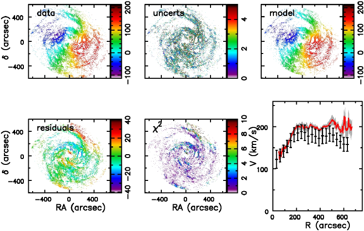
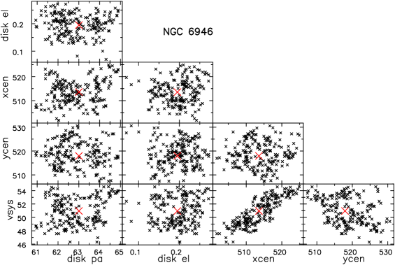
Figure 21: As in Figure 7, but for NGC 6946.

A.15 NGC 6946

Our fitted rotation curve for this galaxy, Figure 21, differs significantly from that given by dB08, especially at radii $>200$″. We also eliminated gas at projected radii $>600$″, which was fitted with still lower circular speeds. The large uncertainties in our estimated circular speeds stem from a significant uncertainty in the fitted inclination, for which the 1-$\sigma$ error is almost 4^∘ (Table 1), and is also reflected in the larger coherent residuals that manifest no tell-tale symmetry. The flat disc assumption in DiskFit is in tension with the steadily varying projection parameters favoured by the rotcur fits dB08. However, our attempts to add a warp to the fitted model made little difference, as DiskFit preferred to apply the warp to the last annulus only.

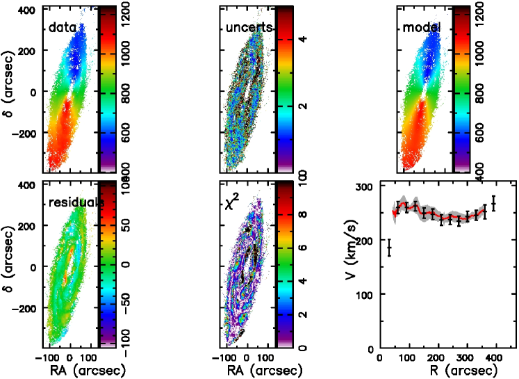
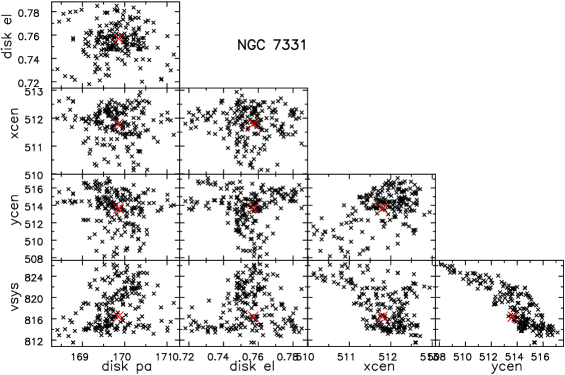
Figure 22: As in Figure 7, but for NGC 7331.

A.16 NGC 7331

Our fit of an axisymmetric flat disc model to this high-mass galaxy, Figure 22, finds a rotation curve in good agreement with the fit from dB08.

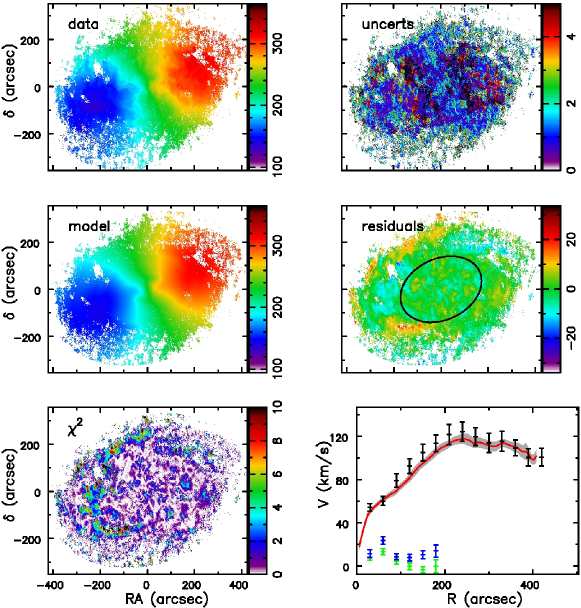
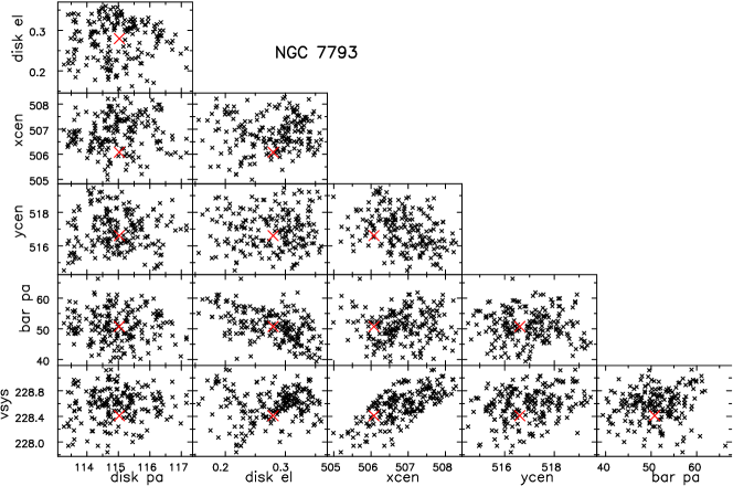
Figure 23: As in Figure 10, but for NGC 7793.

A.17 NGC 7793

The velocity map for this galaxy, Figure 23, is better fitted with a mild oval distortion in the inner parts, as was also found by Sellwood & Zánmar Sánchez (2010). As for NGC 2976, we find that fitting for an inner oval in a flat disc leads to slightly higher estimates of the circular speed over the radial range of the oval than were estimated by dB08, who attributed the inner twisted isovelocity contours to variations in the projection geometry. Otherwise we confirm the somewhat unusual overall rotation curve shape they also reported.

References

- Beers, Flynn & Gebhardt (1990) Beers, T. C., Flynn, K. & Gebhardt, K. 1990, AJ, 100, 32
- Begeman (1989) Begeman, K. G. 1989, A&A, 223, 47
- Bekiaris et al. (2016) Bekiaris, G., Glazebrook, K., Fluke, C. J. & Abraham, R. 2016, MNRAS, 455, 754
- Bosma (1978) Bosma, A. 1978, PhD thesis., University of Groningen
- Bouché et al. (2015) Bouché, N., Carfantan, H., Schroetter, I., Michel-Dansac, L. & Contini, T. 2015, AJ, 150, 92
- Briggs (1990) Briggs, F. H. 1990, ApJ, 352, 15
- Buck et al. (2020) Buck, T., Obreja, A., Macciò, A. V., Minchev, I., Dutton, A. A. & Ostriker, J. P. 2020, MNRAS, 491, 3461
- Burkardt (2017) Burkardt, J. 2017, Website: https://people.sc.fsu.edu/jburkardt/
- Chemin, Carignan & Foster (2009) Chemin, L., Carignan, C. & Foster, T. 2009, ApJ, 705, 1395
- Dame (2011) Dame, T. M. 2011, arXiv:1101.1499
- Davis et al. (2013) Davis, T. A., Alatalo, K., Bureau, M., et al. 2013, MNRAS, 429, 534
- Davis et al. (2017) Davis, T. A., Bureau, M., Onishi, K., Cappellari, M., Iguchi, S. & Sarzi, M. 2017, MNRAS, 468, 4675
- Davis et al. (2020) Davis, T. A., Zabel, N. & Dawson, J. M. 2020, ascl.soft06003
- de Blok (2010) de Blok, W. J. G. 2010, AdAst, 2010, 789293
- de Blok et al. (2008) de Blok, W. J. G., Walter, F., Brinks, E., et al. 2008, AJ, 136, 2648 (dB08)
- de Silva et al. (2015) De Silva, G. M., Freeman, K. C., Bland-Hawthorn, J., et al. 2015, MNRAS, 449, 2604
- de Vaucouleurs et al. (1991) de Vaucouleurs, G., de Vaucouleurs, A., Corwin, H. G., Jr., Buta, R. J., Paturel, G., & Fouqué, P. 1991, Third Reference Catalogue of Bright Galaxies (New York: Springer)
- Di Teodoro & Fraternali (2015) Di Teodoro, E. M. & Fraternali, F. 2015, MNRAS, 451, 3021
- Dutton et al. (2007) Dutton, A. A., van den Bosch, F. C., Dekel, A. & Courteau, S. 2007, ApJ, 654, 27
- Franx, van Gorkom & de Zeeuw (1994) Franx, M., van Gorkom, J. H. & de Zeeuw, T. 1994, ApJ, 436, 642
- Gentile et al. (2006) Gentile, G., Salucci, P., Klein, U., Vergani, D. & Kalberla, P. 2004, MNRAS, 351, 903
- Gerhard (1993) Gerhard, O. E. 1993, MNRAS, 265, 213
- Gunn, Knapp & Tremaine (1979) Gunn, J. E., Knapp, G. R. & Tremaine, S. D. 1979, AJ, 84, 1181
- Haghi et al. (2018) Haghi, H., Khodadadi, A., Ghari, A., Zonoozi, A. H. & Kroupa, P. 2018, MNRAS, 477, 4187
- Hunter et al. (2001) Hunter, D. A., Elmegreen, B. G. & van Woerden, H. 2001, ApJ, 556, 773
- Jörsäter & van Moorsel (1995) Jörsäter, S. & van Moorsel, G. A. 1995, AJ, 110, 2037
- Jòzsa et al. (2007) Jòzsa, G. I. G., Kenn, F., Klein, U. & Oosterloo, T. A. 2007, A&A, 468, 731
- Jòzsa et al. (2009) Jòzsa, G. I. G., Oosterloo, T. A., Morganti, R., Klein, U. & Erben, T. 2009, A&A, 494, 489
- Kamphuis (1993) Kamphuis, J. 1993, PhD thesis., University of Groningen
- Kamphuis et al. (2013) Kamphuis, P., Rand, R. J., Jòzsa, G. I. G., et al. 2013, MNRAS, 434, 2069
- Kamphuis et al. (2015) Kamphuis, P., Jòzsa, G. I. G., Oh, S-H., et al. 2015, MNRAS, 452, 3139
- Katz et al. (2017) Katz, H., Lelli, F., McGaugh, S. S., Di Cintio, A., Brook, C. B. & Schombert, J. M. 2017 MNRAS, 466, 1648
- Lelli, McGaugh & Schombert (2016) Lelli, F., McGaugh, S. S. & Schombert, J. M. 2016, AJ, 152, 157
- Majewski et al. (2017) Majewski, S. R., Schiavon, R. P., Frinchaboy, P. M., et al. 2017, AJ, 154, 94
- Marasco et al. (2019) Marasco, A., Fraternali, F., Heald, G., et al. 2019, A&A, 631, A50
- Marasco et al. (2020) Marasco, A., Posti, L., Oman, K., Famaey, B., Cresci, G. & Fraternali, F. 2020, 2020, A&A, 640, A70
- Oh et al. (2008) Oh, S-H., de Blok, W. J. G., Walter, F., Brinks, E. & Kennicutt, R. C., Jr. 2008, AJ, 136, 2761
- Oh et al. (2011) Oh, S-H., Brook, C., Governato, F., Brinks, E., Mayer, L., de Blok, W. J. G., Brooks, A. & Walter, F. 2011, AJ, 142, 24
- Oh et al. (2019) Oh, S-H., Staveley-Smith, L. & For, B-Q. 2019, MNRAS, 485, 5021
- Oman et al. (2015) Oman, K. A., Navarro, J. F., Fattahi, A., et al. 2015, MNRAS, 452, 3650
- Oman et al. (2019) Oman, K. A., Marasco, A., Navarro, J. F., Frenk, C. S., Schaye, J. & Benítez-Llambay, A. 2019, MNRAS, 482, 821
- Ponomareva et al. (2016) Ponomareva, A. A., Verheijen, M. A. W. & Bosma, A. 2016, MNRAS, 463, 4052
- Posti et al. (2019) Posti, L., Marasco, A., Fraternali, F. & Famaey, B. 2019, A&A, 629, A59
- Press et al. (1992) Press, W. H., Flannery, B. P., Teukolsky, S. A. & Vetterling, T. A. 1992, Numerical Recipes (Cambridge: Cambridge Univ. Press)
- Rogstad, Lockhart & Wright (1974) Rogstad, D. H., Lockhart, I. A. & Wright, M. C. H. 1974, ApJ, 193, 30
- Rots et al. (1990) Rots, A. H., Bosma, A., van der Hulst, J. M., Athanassoula, E. & Crane, P. C. 1990, AJ, 100, 387
- Schoenmakers et al. (1997) Schoenmakers, R. H. M., Franx, M. & de Zeeuw, P. T. 1997, MNRAS, 292, 349
- Sellwood (2013) Sellwood, J. A. 2013, in Planets Stars and Stellar Systems, v.5, eds. T. D. Oswalt & G. Gilmore (Heidelberg: Springer) p. 923 (arXiv:1006.4855)
- Sellwood & Spekkens (2015) Sellwood, J. A. & Spekkens, K. 2015, arXiv:1509.07120