Learning Anthropometry from Rendered Humans

Abstract

Accurate estimation of anthropometric body measurements from RGB imags has many potential applications in industrial design, online clothing, medical diagnosis and ergonomics. Research on this topic is limited by the fact that there exist only generated datasets which are based on fitting a 3D body mesh to 3D body scans in the commercial CAESAR dataset. For 2D only silhouettes are generated. To circumvent the data bottleneck, we introduce a new 3D scan dataset of 2,675 female and 1,474 male scans. We also introduce a small dataset of 200 RGB images and tape measured ground truth. With the help of the two new datasets we propose a part-based shape model and a deep neural network for estimating anthropometric measurements from 2D images. All data will be made publicly available.

1 Introduction

Recovery of 3D human body from 2D images is an important yet challenging problem with many potential applications in industrial design [28], online clothing [11], medical diagnosis [27] and work ergonomics [30]. However, compared to pose estimation, less attention has been paid on the task of accurate shape estimation, especially from RGB images. Due to the lack of public datasets, previous works [14, 12, 13, 7, 10, 9, 8, 37, 46] adopt the strategy of creating synthetic samples with shape models, e.g. SMPL [24] and SCAPE [3], and reconstruct body shapes from generated 2D silhouettes. Recent works [16, 6, 21, 20, 19, 29] consider to directly estimate human bodies from RGB images, but the works focus on 3D pose estimation.

Vision based anthropometry has many potential applications in clothing industry, custom tailoring, virtual fitting and games. The state-of-the-art works [14, 12, 13] recover 3D body surfaces from silhouettes and obtain the anthropometric measurements as by-products. There does not exist an RGB dataset for evaluation and HS-Net in [12] and HKS-Net in [13] are evaluated only on 4-7 real samples.

To tackle the task of accurate anthropometric measurement estimation from RGB images, we directly regress 2D images to body measurements using a deep network architecture which omits the body reconstruction stage. However, we also provide a 3D body mesh by learning a mapping from the measurements to the shape coefficients of a part-based shape model. For network training and shape model building, we introduce a new dataset of 3D body scans. For training we render virtual RGB bodies consistent with the true data. To evaluate measurement prediction for real cases, we also release a testing RGB dataset of 200 real subjects and their tape measurements as ground truth. The proposed network, trained with generated data, provide anthropometric measurements with state-of-the-art accuracy as compared to the previous works on the existing [48, 32] and the new introduced data.

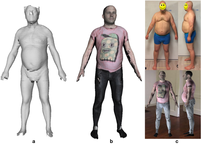
Figure 1: Contributions of this work: a) 4,149 3D body scans; b) fitted body meshes with textures; and c) real (top) and rendered (bottom) RGB images for training anthropometric measurement network architectures.

Contributions of our work are the following:

• a dataset of 2,675 female and 1,474 male scans,

• A dataset of 200 RGB images of real subjects with tape measured ground truth;

• an anthropometric body measurement network architecture trained with rendered images.

In the experiments our network achieves competitive performances on both tasks of anthropometric measurement estimation and body shape reconstruction compared to the state-of-the-art works.

2 Related work

Datasets. CAESAR dataset [33] is a commercial dataset of human body scans and tape measured anthropometric measurements and its lisence prevents public usage. Yang et al. [48] and Pischulin et al. [32] fitted 3D body templates to the CAESAR scans and used the fitted meshes and geodesic distances in their experiments. Some of the fitted meshes are available in their project pages. Another popular option has been to use synthetic data, for example, SURREAL [40] consists of synthetic 3D meshes and RGB images rendered from 3D sequences of human motion capture data and by fitting the SMPL body model [24]. Realistic dataset with RGB images and tape measured ground truth is not available. In this work we use the fitted CAESAR meshes [48], namely CAESAR fits.

Shape models. The body shape variation is typically captured by principal component analysis (PCA) on registered meshes of a number of subjects, such as the 3D scans in the commercial CAESAR dataset [33]. For example, Allen et al [1] fit a template to a subset of CAESAR dataset and model the body shape variation by PCA. Seo et al. [35] adopt the same approach in their characterization of body shapes. SCAPE [3] is one of the most popular shape models used in similar works to ours. SCAPE decomposes shape to pose invariant and pose dependent shape components to perform more realistic deformations. Yang et.al [48] utilize the SCAPE model to learn the shape deformation and introduce a local mapping method from anthropometric measurements (”semantic parameters”) to shape deformation parameters. Another popular shape model is SMPL [24] which also decomposes shape into pose dependent and independent parts. SMPL shape variation is also learned from the CAESAR data, but provides better details than SCAPE. The public version of the SMPL model provides only 10 PCA components preventing reconstruction of local details.

One drawback of PCA based shape modelling is the fact that PCA vectors represent global deformation and important details of local parts such as upper torso or pelvis can be missing (Figure 2). There exists a number of shape models that provide local deformations. For example, Zuffi et al. [50] introduce a part-based model in which each body part can independently deform. Similarly Bernard et al. and Neumann et al. [5, 26] extract sparse and spatially localized deformation factors for better local shape deformation.

Auxiliary information, such as the qualitative body type, has been added to the shape parameters in several works [1, 38, 34, 35, 48].

Shape estimation Due to the lack of real RGB datasets, previous works [7, 10, 9, 8, 37, 46, 13, 12, 14, 18, 36] reconstruct 3D body meshes from 2D silhouettes. The silhouettes are generated using the CAESAR fits or using synthetic body models. The early works extract handcrafted silhouette features which are mapped to 3D shape parameters using, e.g., the linear mapping [46], a mixture of kernel regressors [37], Random Forest Regressors [14, 10], or a shared Gaussian process latent variable model [9, 8]. The more recent works [12, 13, 18] propose deep network architectures to estimate the shape model parameters in an end-to-end manner.

A number of pose estimation methods also provide a 3D shape estimate [16, 6, 21, 20, 19, 29], but shape is only coarse and anthropometric measurements made on them are inaccurate (see our experiments). In these works, a parametric 3D model is fitted to silhouettes [17], certain body keypoints or joints [6], or a collection of 2D observations [16, 21]. For example, given the subject’s height and a few clicked points, Guan et al. [16] fits the SCAPE model to the image and fine-tuners the result using silhouettes, edges and shadings. Kanazawa et al. [19] propose an end-to-end adversarial learning framework to recover 3D joints and body shapes from a single RGB image by minimizing the joint reprojection error. Kolotouros et al. [29] extend SMPLify [6] by neural network based parameter initialisation and iterative optimization. To estimate 3D human shapes from measurements, [45] first optimize the shape of a PCA-based model to find the landmarks that best describe target measurements and then deform the shape to fit the measurements.

Anthropometric measurements. Previous works [39, 44, 25, 43, 47] predict measurements from 3D human scans with the help of 3D body models which provide the correspondences. They first register a template to scans, then obtain the lengths of measurement paths defined by the vertices on the template surface (geodesic distances). From registered meshes, Tsoli et al. [39] extract the global and local features, including PCA coefficients of triangle deformations and edge lengths, the circumferences and limb lengths, then predicts measurements from these features using regularized linear regression. To eliminate negative effects caused by varying positions of measurement paths across subjects, [47] obtains the optimal result through a non-linear regressor over candidate measurements extracted from several paths in the same area.

There exists a few works estimating anthropometric measurements from 2D images. Most works [41, 7, 12, 13, 23] first construct a shape model and then obtain measurements from reconstructed bodies. Another line of works [4, 15, 42, 22] estimate the circumferences of body parts using fiducial points on the contours. For example, in [4] part circumferences are estimated using an ellipsoid model and lengths between two relevant fiducial points from the frontal and lateral views of silhouettes.

To the authors’ best knowledge our work is the first attempt to estimate accurate anthropometric measurements from RGB images.

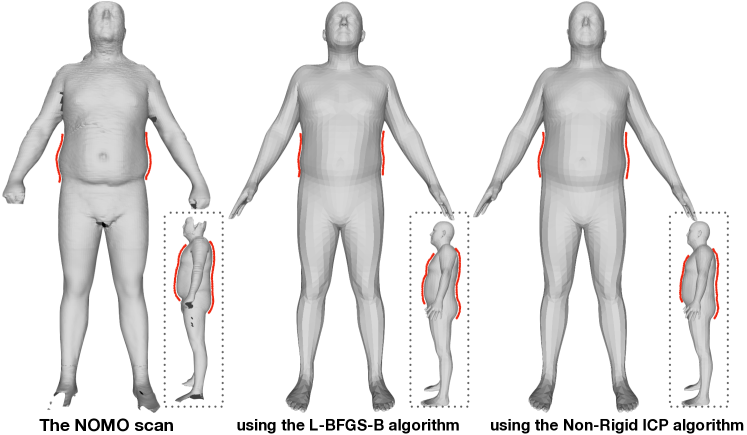
Figure 2: Left: an original scan of a subject. Middle: SMPL fit using the L-BFGS-B algorithm [49]. Right: the registered mesh using Non-Rigid ICP algorithm [2]. Red curves mark the local areas where the two methods particularly differ from each other.

3 Methodology

3.1 Datasets

Rendered RGB. We collected a dataset of real body scans, namely XXXX-scans dataset, captured by a commercial TC2 system. 1,474 male and 2,675 female subjects were scanned. The scanned subjects were instructed to take approximate “A”-pose and held the capturing device handles. The quality of the scans vary and in many of the scans point regions are missing near feet, hand and head. To construct watertight meshes an SMPL template in the ”A”-pose was fitted using the non-rigid ICP method of Amberg et al. [2] (Fig 1 a-b & Fig 2 Right). The fitted XXXX-scans dataset is called as XXXX-fits.

Finally, a set of rendered RGB images were generated from the XXXX-fits meshes using the rendering method in SURREAL [40]. Each image was generated using a randomly selected home background, body texture (clothes and skin details), lighting and a fixed camera position. RGB images were generated from the both frontal and lateral views (Figure 1 c (bottom)).

Real RGB. We collected a dataset of RGB images of 200 volunteers using iPhone 5S rear camera (Figure 1 c (top)), namely XXXX-real-200. All volunteers wear only underwear and photos were captured indoors. The approximate capturing distance was 2.4 m and the camera height from the ground 1.6 m. The anthropometric measurements were done using a tape measure by a tailoring expert.

3.2 Part-based Shape Model

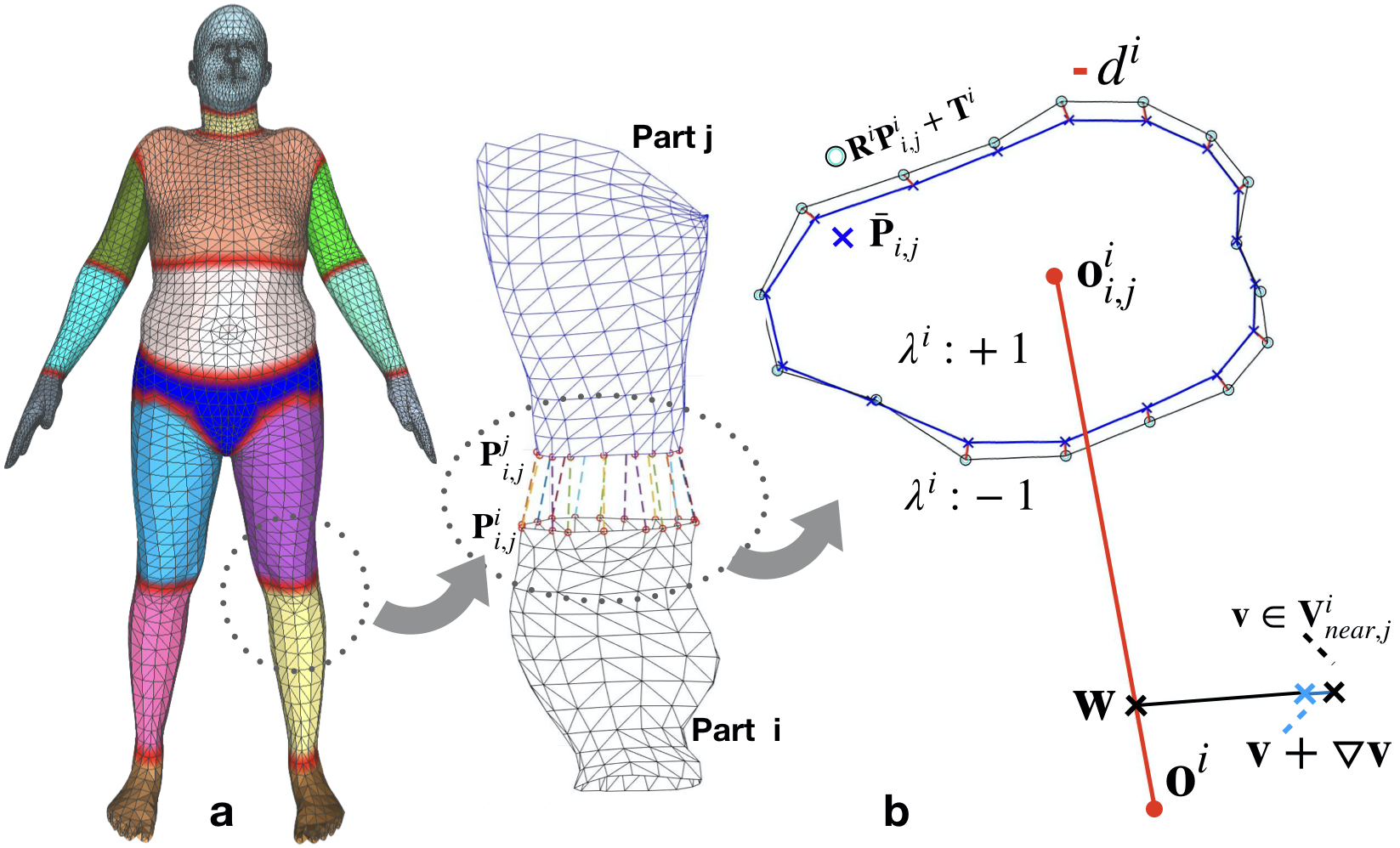
Figure 3: The Body Segments (a) and the Stitching Process (b). Details of the stitch deformation are illustrated in Sec 3.2. Red markers in (a) denote the interface points.

Since in our scenario the subject is volunteering and takes a pre-defined pose it can be safely assumed that decomposition of the shape to pose specific and pose invariant components is not needed. To capture local details, we adopt a part-based body model to be able to model shape variation of each part with the same accuracy. The proposed model is composed of 17 body parts: head, neck, upper torso, lower torso, pelvis, upper legs, lower legs, upper arms, lower arms, hands and feet (Figure 3 a). Each part is a triangulated 3D mesh in a canonical, part-centered, coordinate system.

Part-based Shape Model.

The SP model [50] first applies PCA over the full body and then defines a PCA component matrix for each part by grouping part specific rows in the shape basis matrix. Instead we directly apply PCA on each body part to model its shape variance. Let $\mathbb{X}^{i}$ be the mesh vertices for the part $i$, a part instance is generated by adjusting the shape parameters $\mathbb{\beta}^{i}$ as

$$\mathbb{X}^{i}=\mathbb{U}^{i}\mathbb{\beta}^{i}+\mathbb{\mu}^{i}$$ (1)

where $\mathbb{U}^{i}$ is the PCA component matrix and $\mathbb{\mu}^{i}$ is the mean intrinsic shape across all training shapes.

Part Stitching.

Inspired by [50], we also define interface points $\mathbb{P}_{i,j}$ that are shared by two neighbor parts $i$ and $j$. The stitching process (see Figure 3 b) starts from the root node (the pelvis) and stitches the part $i$ with its parent $j$ using the rotation matrix $\mathbb{R}^{i}$ and translation matrix $\mathbb{T}^{i}$. Translation and rotation are solved as the Orthogonal Procrustes transformation:

$$\begin{split}\mathbb{R}^{i}~{}~{}&=\operatorname*{argmin}_{\Omega}||\mathbb{\Omega}\mathbb{P}^{i}_{i,j}-\mathbb{P}^{j}_{i,j}||_{F},~{}s.t.~{}\Omega^{T}\Omega=I\\ \mathbb{T}^{i}~{}~{}&=\mathbb{o}^{j}_{i,j}-\mathbb{o}^{i}_{i,j}\end{split}$$ (2)

where $\mathbb{P}^{i}_{i,j}$, $\mathbb{P}^{j}_{i,j}$ denote the interface points on the part $i$ and $j$ respectively, and $\mathbb{o}^{i}_{i,j}$, $\mathbb{o}^{j}_{i,j}$ indicate the centers of the interface points and $\mathbb{X}^{i,align}$, $\mathbb{P}^{i,align}_{i,j}$ represent the aligned mesh vertices and the interface points of part $i$. We adopt $\bar{\mathbb{P}}_{i,j}=(\mathbb{P}^{i,align}_{i,j}+\mathbb{P}^{j}_{i,j})/2$ as the final interface points.

Neighbor parts of the same body should be stitched seamlessly. Hence we introduce the stitch deformation to smooth the stitched areas. Consider the part $i$ as the example, we calculate the mean deformation distance $\triangledown d^{i}$ and the deformation direction $\lambda^{i}$ as follows:

$$\begin{split}\triangledown d^{i}&=\frac{1}{|\bar{\mathbb{P}}_{i,j}|}\sum^{|\bar{\mathbb{P}}_{i,j}|}_{k=1}dist(\mathbb{\bar{p}}^{i}_{k},\mathbb{p}^{i,align}_{k})\\ \lambda^{i}&=\bigg{\{}\begin{array}[]{l}-1,~{}~{}if~{}\frac{1}{N}\sum^{N}_{k=1}\measuredangle\mathbb{o}^{i}_{i,j}\mathbb{\bar{p}}^{i}_{k}\mathbb{p}^{i,align}_{k}\leq\frac{\pi}{2}\\ +1,~{}~{}otherwise\end{array}\end{split}$$ (3)

where $\mathbb{\bar{p}}^{i}_{k}$, $\mathbb{p}^{i,align}_{k}$ are the k-th points of $\bar{\mathbb{P}}_{i,j}$ and $\mathbb{P}^{i,align}_{i,j}$. $\lambda^{i}$ indicates the deformations towards inside or outside.

Let $\mathbb{o}^{i}$ be the center of part $i$, $\mathbb{v}\in\mathbb{V}^{i}_{near,j}$ be a random vertex near by the interface area, and $\mathbb{w}$ be a point on the line segment $\mathbb{o}^{i}\mathbb{o}^{i}_{i,j}$ and ${\overrightarrow{\mathbb{v}\mathbb{w}}}\perp{\small{{\overrightarrow{\mathbb{o}^{i}\mathbb{o}^{i}_{i,j}}}}}$. The deformation $\triangledown\mathbb{v}$ at vertex $\mathbb{v}$ can be presented as:

$$\begin{split}\triangledown\mathbb{v}&=\lambda^{i}*\frac{\overrightarrow{\mathbb{v}\mathbb{w}}}{|\overrightarrow{\mathbb{v}\mathbb{w}}|}*\frac{|\overrightarrow{\mathbb{o}^{i}_{i,j}\mathbb{w}}|}{|\overrightarrow{\mathbb{o}^{i}\mathbb{o}^{i}_{i,j}}|}*\triangledown d^{i}\\ \mathbb{V}^{i}_{near,j}&=\{\mathbb{v}|\frac{|\overrightarrow{\mathbb{o}^{i}_{i,j}\mathbb{w}}|}{|\overrightarrow{\mathbb{o}^{i}\mathbb{o}^{i}_{i,j}}|}\leq\epsilon,for~{}\mathbb{v}\in\mathbb{X}_{i}\}\end{split}$$ (4)

where $\mathbb{V}^{i}_{near,j}$ denotes the neighbour vertices of the interface points $\mathbb{P}^{i}_{i,j}$, and $\epsilon$ is set to 0.1 in our experiments.

3.3 Virtual Tailor Body Measurements

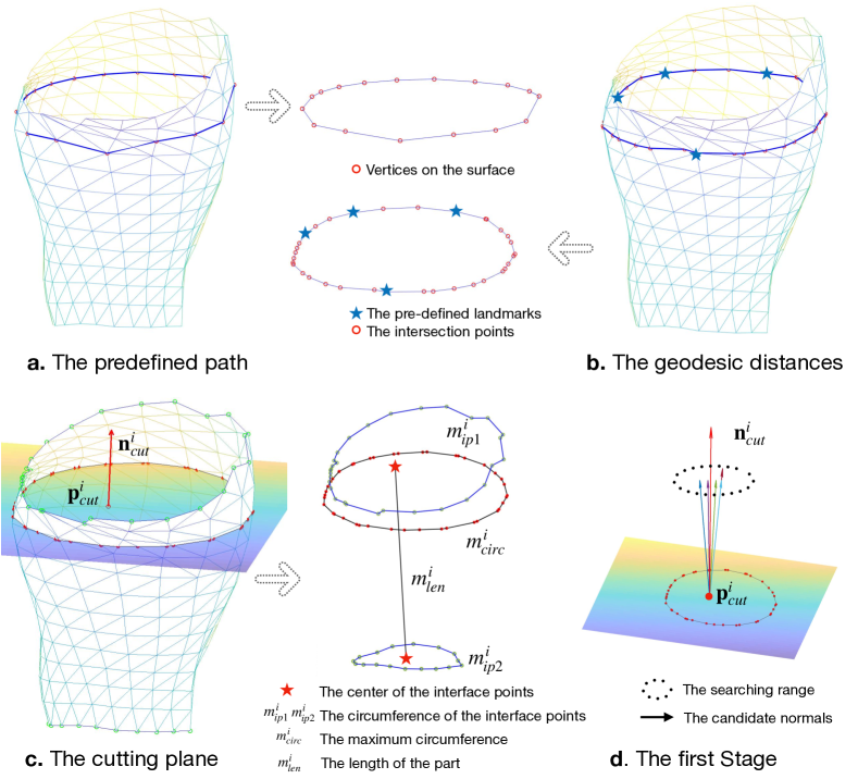
Figure 4: Various types of virtual tailor body measurements: a) a predefined path consisting of a set of vertices; b) a geodesic path through a set of pre-defined landmarks; c) a perimeter of the plane section (proposed); d) the first stage of the proposed procedure finds the normal of the cutting plane.

Accurate anthropometric body measurements are the final goal of vision based body shape analysis. Therefore it is important how these are defined when trained with 3D model rendered images. In prior arts there have been two dominating practices (Figure 4): i) predefined paths consisting of a set of vertices [47]; ii) geodesic distances through pre-defined landmarks [7, 12, 13]. The first method sums edge lengths between the pre-defined vertices. However, due to the non-rigid ICP model fitting procedure the vertex positions can be heavily deformed and the paths do not anymore correspond to the shortest path used by the tailors. The second method defines a number of landmarks along the circumference paths, but also the landmarks suffer from fitting deformations. In order to provide measurements that better match the tailor procedure, we propose an alternative measurements. Our procedure first aligns the body mesh rotation and then uses a cutting plane to define a circumference path without deformations.

The perimeter of the surface along the plane section of each body part $i$ is adopted as the circumference measure $m^{i}_{circ}$ of that part. The cutting plane is determined by the cutting point $\mathbb{p}^{i}_{cut}$ and the normal $\mathbb{n}^{i}_{cut}$. The whole process (Figure 4 c-d) consists of two stages. The first stage finds the normal $\mathbb{n}^{i}_{cut}$ which minimizes the circumference $m^{i}_{circ}$ at the certain cutting point. This stage forces the cutting plane to be perpendicular to the body part. Finding the cutting point $\mathbb{p}^{i}_{cut}$ which maximizes the circumference $m^{i}_{circ}$ is done by sampling in a certain range in the second stage.

Besides the circumference $m^{i}_{circ}$, we also define the length $m^{i}_{len}$ of the body part and the circumferences $m^{i}_{ip1},m^{i}_{ip2},...m^{i}_{ipN}$ of the interface points. The measurements of the body part $i$ are $\mathbb{m}^{i}=[m^{i}_{circ},m^{i}_{len},m^{i}_{ip1},m^{i}_{ip2},...m^{i}_{ipN}]^{T}$

3.4 From Body Measurements to Body Shape

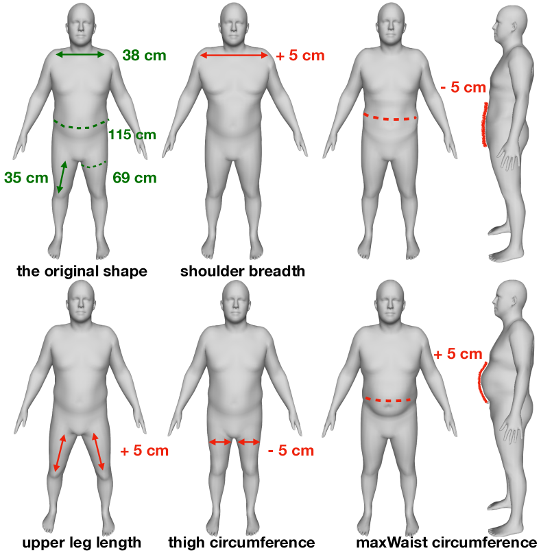
Figure 5: Editing the shape by updating the body measurements. Green numbers denote the original body measurements. Red numbers denote increasing or decreasing these measurements.

Similar to [1, 48], we learn mapping from the body measurements $\mathbb{m}^{i}$ to the PCA shape variables $\mathbb{\beta}^{i}$. This is done separately for each body part using

$$[m^{i}_{circ},m^{i}_{len},m^{i}_{ip1},...m^{i}_{ipN},1]^{T}\mathbb{F}^{i}=\mathbb{\beta}^{i}$$ (5)

Using the training set, the computed measurements and shape parameters are put into data matrices $\mathbb{M}^{i}$ and $\mathbb{B}^{i}$ and the transformation matrix $\mathbb{F}^{i}$ is computed in the least-square sense as

$$\mathbb{F}^{i}=\mathbb{M}^{i,+}\mathbb{B}^{i}$$ (6)

where ⁺ denotes the pseudo-inverse operation. Given a new set of body measurements $\mathbb{m}$, we can obtain the PCA coefficients from $\mathbb{b}=\mathbb{m}\mathbb{F}$.

Finally, mapping from the anthropometric measurements to body shapes allows more intuitive generation of training samples as the measurements can be varied $\pm\Delta\mathbb{m}$ and the corresponding body shapes generated (Figure 5).

3.5 Anthropometric Measurements Network

To tackle the task of estimating accurate anthropometric measurements from silhouettes or RGB images, we introduce a deep neural network architecture (Figure 6). Unlike the previous works [14, 12, 13, 6] whose primary task is body shape reconstruction, our network aims at learning a mapping from shape descriptors to anthropometric measurements. Our network consists of two components: 5 convolutional layers to compute deep features for RGB or silhouette input and 6 fully-connected layers to map the deep features to anthropometric body measurements. The network can be trained with multiple inputs, but only two (frontal + side) were included to the experiments. The subject height and virtual camera calibration parameters were used to scale and center the subject into an image of resolution $480\times 200$. There is no weight sharing between the inputs to allow network to learn a view specific features. For multiple inputs, a merge layer is applied to correlate the multiple view features before the regression layer.

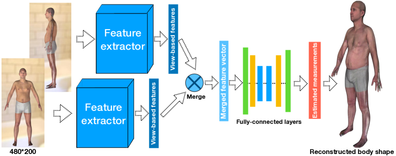
Figure 6: The proposed Anthropometric Measurements Network.

4 Experiments

Data Preparation We run experiments on two different datasets, XXX-fits and CAESAR-fits [48]. The training and test samples are split equally for each dataset. In order to generate a large number of training samples for network training, the PCA-based statistical shape model constructed from the training samples is used to generate 10K training examples of various shapes.

For each body part, the PCA is applied separately and the first four principal components covering about $92\%$ of shape variance are selected for learning the linear mapping to corresponding body measurements.

Network Training & Evaluation The proposed network learns mapping from RGB images to 34 anthropometric measurements. The network is trained with the Adadelta optimizer using the learning rate $10^{-4}$. The network uses the standard MSE loss and is trained 100 epochs.

4.1 Results

Quantitative Experiments For comparison, the state-of-the-art methods, HKS-Net [13], HMR [19] and SMPLify [6] are trained with the same data and compared to the proposed network. HKS-Net uses the UF-US-2 architecture and was trained with RGB images. HMR [19] and SMPLify [6] use only the frontal RGB image. For SMPLify [6] the estimated locations of joints by DeepCut [31] are provided and the original models of [6] and [19] were used. The mean measurement errors on reconstructed meshes are reported in Table 1 & 2 and illustrations of the results are provided in the supplementary material. Our method achieves competitive performance compared to the state-of-the-arts works on both two dataset. Our method shows significantly better performances on the upper torso (chest, waist and pelvis). The error distributions over these measurements for our method and HKS-Net on XXX-fits dataset are plotted in Figure 7.

Measurements	Ours	HKS	HMR	SMPLify
a. Head Circumference	24.9	24.3	25.2	33.0
b. Neck Circumference	14.5	15.8	25.3	22.4
c. Shoulder-crotch Len.	14.8	13.2	25.7	63.4
d. Chest Circumference	34.4	40.8	92.7	67.3
e. Waist Circumference	36.7	50.3	88.7	74.8
f. Pelvis Circumference	23.9	28.4	56.2	89.3
g. Wrist Circumference	7.9.	7.3	11.0	9.9
h. Bicep Circumference	13.5	15.1	37.7	26.4
i. Forearm Circumference	9.3	9.7	16.1	20.6
j. Arm length	7.5	5.9	24.5	138.0
k. Inside Leg length	12.9	10.0	36.3	229.6
l. Thigh Circumference	19.6	21.6	36.4	44.8
m. Calf Circumference	11.2	12.7	19.7	22.5
n. Ankle Circumference	7.5	7.5	10.7	23.2
o. Overall height	29.8.	23.2	92.9	419.5
p. Shoulder breadth	8.6	7.9	19.9	68.4

Table 1: Experiments on RGB images of the XXX-fits dataset. Mean absolute errors (MAE) of body measurements are reported in millimeters. Ours network predicts the body measurements, HKS-Net [13] adopts the UF-US-2 architecture; HMR [19] and SMPLify [6] take only the frontal views. SMPLify requires estimated joints from DeepCut [31].

Measurements	Ours	HKS	HMR	SMPLify
a. Head Circumference	11.6	10.8	16.3	28.1
b. Neck Circumference	12.3	13.1	27.2	24.4
c. Shoulder-crotch Len.	13.9	13.4	28.6	57.8
d. Chest Circumference	26.1	28.3	68.3	74.5
e. Waist Circumference	28.7	38.6	85.3	72.8
f. Pelvis Circumference	22.6	26.0	62.8	99.1
g. Wrist Circumference	6.9	6.5	14.3	11.9
h. Bicep Circumference	13.0	13.4	35.6	28.4
i. Forearm Circumference	7.8	8.0	16.7	25.9
j. Arm length	9.5	6.9	45.3	150.2
k. Inside Leg length	11.2	8.7	37.2	219.1
l. Thigh Circumference	18.2	18.5	39.3	51.3
m. Calf Circumference	11.7	11.8	21.4	28.4
n. Ankle Circumference	7.8	7.9	13.6	28.8
o. Overall height	20.1.	11.8	96.5	398.5
p. Shoulder breadth	7.6	7.7	21.8	51.9

Table 2: Experiments on RGB images of CAESAR-fits dataset. MAEs of body measurements are reported in millimeters.

Qualitative Experiments We evaluate related methods on the XXX-real-200 dataset. Visualizations of some estimated body shapes are shown in Figure 10. Our reconstructions (the second column) restore finer local details, as compared to previous works [19, 13, 6]. Our method can be directly applied on the RGB images rather than converting images into binary silhouettes and does not require additional information, e.g. the estimated joints.

The bottom row in Figure 10 shows the failure case due to wrong estimation on the lengths of upper torso and pelvis, which leads to the unnatural ratio of upper body. Interestingly similar mistakes happen in other methods.

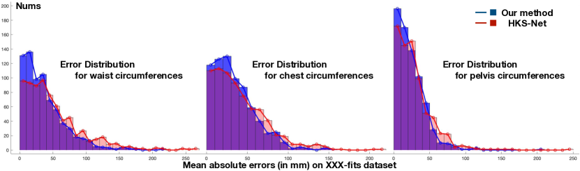
Figure 7: Analysis of measurement errors for our method and HKS-Net on XXX-fits dataset. Left: the error distribution for waist circumference; Middle: the error distribution for chest circumference; Right: the error distribution for pelvis circumference.

Different background images Considering about the effects brought by the background images, we evaluated the proposed network on the XXX-fits and CAESAR-fits datasets of which images are rendered with 4 types of background images: clear images, blurry images, random noisy images, and pure black images. The mean measurement errors are illustrated in Table 3 and Figure 8, and illustrations of the results are in the supplementary material. Our network shows the robustness to complicated background images. Binary silhouettes inputs provide the best results and the performance drops when the background getting complicated. Background images, lighting, and cloths do bring negative effects and methods for background removal would promote the performance of anthropometric measurements estimation. However, due to the imperfection of silhouette extraction algorithms, it become difficult to obtain such perfect silhouettes.

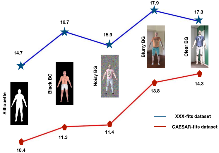
Figure 8: Our proposed method is evaluated on XXX-fits and CAESAR-fits datasets with different background images . Mean errors of all 16 measurements (in mm) are plotted.

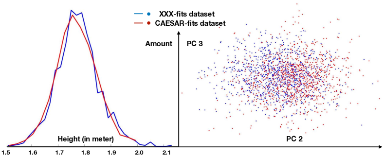
Figure 9: Shape spaces of XXX-fits and CAESAR-fits datasets. Left: the distributions of height data. Right: the first 2 PCA coefficients of shapes.

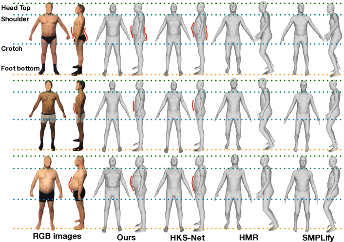
Figure 10: The Qualitative Experiments on XXX-real-200 dataset. Dash lines mark four meaningful locations: head top, shoulder, crotch point, and foot bottom. Red lines mark the local areas where these methods particularly differ from each other. Bottom row shows the failure case due to the wrong estimations on the pelvis and upper torso.

Evaluation on Reconstructed bodies. In our work, body shapes are recovered from estimated anthropometric measurements with the help of a part-based shape model (Sec 3.4). To illustrate the advantage of proposed part-based shape model, we train another network predicting totally 68 PCA coefficients for all parts. The results of mean measurement errors on the reconstructed body surfaces are illustrated in Table 4. As shown, the linear mapping method restores the bodies in good qualities without losing local details compared to the network estimating PCA coefficients.

Analysis of shape datasets. To visualize high dimensional PCA shape spaces of the XXX-fits and CAESAR-fits datasets, we merge two datasets and perform PCA on these body meshes then select the first 10 PCA coefficients as the feature vectors and standardize them to have zero mean and unit variance. To supply a lower-dimensional picture, we select the first 3 principle coefficients as the coordinates of body shapes. Since the first principle component encodes the height information, we plot the distributions of height data from two datasets in Figure 9. Then the second and third principal coefficients are tread as the 2D coordinates. Two datasets capture different shape variances and our proposed XXX-fits dataset contributes the considerable body shapes for related datasets and works.

Discussion and Future works A limitation to our method is that the body shape is reconstructed from 34 measurements covering the whole body. One challenge task is how to recover body shape from fewer (less than 34) measurements. The correlation among anthropometric measurements would to be explored in future work.

Another one of future work is to consider how to narrow the gap between the self-defined measurements and tape measurements in related applications. The gaps among different kinds of measurements are noticeable: the self-defined body measurements of XXX-fits dataset (Sec 4), the TC2 measurements of XXX-scans dataset from the TC2 system and tape measurements of XXX-real-200 dataset. For real applications, tape measurements are the foremost target and necessary procedures are required for domain adaption. In our experiments a non-linear regressor was trained on XXX-real-200 dataset for domain transfer, however, it is still insufficient to meet strict industrial requirements. Analysis of measurement errors is illustrated in the supplementary material. More data and works on vision-based anthropometry are needed in future work.

5 Conclusions

We posed the task of anthropometric measurements estimation as regression by learning a mapping from 2D image clues to body measurements, and reconstruct body shapes from predicted measurements. The proposed method was evaluated on thousands of human bodies (XXX-fits and CAESAR-fits datasets) and 200 real subjects (XXX-real-200 dataset). To the authors’ best knowledge the proposed dataset is the first freely available dataset of real human body shapes along with the measurements. Further more, we evaluated the proposed method with images in different backgrounds and showed its robustness to the influence of noise of backgrounds, lighting and cloths .

Measurements & Datasets	XXX-fits		CAESAR-fits
	RGB	Silh.	RGB	Silh.
a. Head Circumference	24.9	22.8	11.6	10.4
b. Neck Circumference	14.5	14.4	12.3	10.6
c. Shoulder-crotch Len.	14.8	12.4	13.9	12.9
d. Chest Circumference	34.4	22.2	26.1	15.3
e. Waist Circumference	36.7	32.9	28.7	15.0
f. Pelvis Circumference	23.9	23.8	22.6	17.0
g. Wrist Circumference	7.9	7.4	6.9	6.3
h. Bicep Circumference	13.5	10.6	13.0	9.9
i. Forearm Circumference	9.3	7.7	7.8	6.2
j. Arm length	7.5	5.4	9.5	6.4
k. Inside Leg length	12.9	8.5	11.2	7.1
l. Thigh Circumference	19.6	18.9.	18.2	12.8
m. Calf Circumference	11.2	11.7	11.7	10.6
n. Ankle Circumference	7.5	7.1	7.8	7.2
o. Overall height	29.8	21.9	20.1	12.4
p. Shoulder breadth	8.6	6.9	7.6	6.0

Table 3: The results of our proposed method with RGB images and binary silhouettes on XXX-fits and CAESAR-fits datasets. Mean absolute errors of body measurements are reported in millimeters.

Datasets	XXX-fits			CAESAR-fits
Meas.	Part-PCA	Meas-1	Meas-2	Part-PCA	Meas-1	Meas-2
a.	23.1	23.0	24.9	10.7	11.3	11.6
b.	15.4	14.5	14.5	12.1	12.1	12.3
c.	18.5	18.7	14.8	16.1	16.4	13.9
d.	33.5	34.4	34.4	26.9	26.0	26.1
e.	45.0	36.5	36.7	32.2	28.5	28.7
f.	26.6	23.9	23.9	23.4	22.8	22.6
g.	7.1	7.2	7.9	6.5	6.8	6.9
h.	13.0	13.6	13.5	12.2	13.0	13.0
i.	8.9	9.1	9.3	7.6	8.0	7.8
j.	6.0	7.6	7.5	7.0	9.5	9.5
k.	10.2	13.0	12.9	8.2	11.2	11.2
l.	20.0	19.7	19.6	16.9	18.2	18.2
m.	11.8	11.2	11.2	11.4	11.7	11.7
n.	7.5	7.5	7.5	7.7	7.8	7.8
o.	25.7	32.1	29.8	17.5	21.9	20.1
p.	9.0	9.1	8.6	7.3	7.7	7.6

Table 4: Evaluation on the accuracy of reconstructed body shapes. Mean absolute errors (MAE) of body measurements on the reconstructed body surfaces are reported in millimeters. Part-PCA denotes the body shapes are reconstructed by the PCA coefficients for body parts (Sec 3.2); Meas-1 denotes that the network directly predicts the body measurements and body shapes are reconstructed through the linear mapping (Sec 3.4); Meas-2 denotes the MAE of the predicted measurements.

References

- [1] Brett Allen, Brian Curless, Brian Curless, and Zoran Popović. The space of human body shapes: reconstruction and parameterization from range scans. In ACM transactions on graphics (TOG), volume 22, pages 587–594. ACM, 2003.
- [2] Brian Amberg, Sami Romdhani, and Thomas Vetter. Optimal step nonrigid ICP algorithms for surface registration. In CVPR, 2007.
- [3] D. Anguelov, P. Srinivasan, D. Koller, S. Thrun, J. Rodgers, and J. Davis. SCAPE: shape completion and animation of people. In SIGGRAPH, 2005.
- [4] Murtaza Aslam, Fozia Rajbdad, Shahid Khattak, and Shoaib Azmat. Automatic measurement of anthropometric dimensions using frontal and lateral silhouettes. IET Computer Vision, 11(6):434–447, 2017.
- [5] Florian Bernard, Peter Gemmar, Frank Hertel, Jorge Goncalves, and Johan Thunberg. Linear shape deformation models with local support using graph-based structured matrix factorisation. In Proceedings of the IEEE Conference on Computer Vision and Pattern Recognition, pages 5629–5638, 2016.
- [6] Federica Bogo, Angjoo Kanazawa, Christoph Lassner, Peter Gehler, Javier Romero, and Michael J. Black. Keep it SMPL: Automatic estimation of 3D human pose and shape from a single image. In Computer Vision – ECCV 2016, Lecture Notes in Computer Science. Springer International Publishing, Oct. 2016.
- [7] Jonathan Boisvert, Chang Shu, Stefanie Wuhrer, and Pengcheng Xi. Three-dimensional human shape inference from silhouettes: reconstruction and validation. Machine vision and applications, 24(1):145–157, 2013.
- [8] Yu Chen and Roberto Cipolla. Learning shape priors for single view reconstruction. In Computer Vision Workshops (ICCV Workshops), 2009 IEEE 12th International Conference on, pages 1425–1432. IEEE, 2009.
- [9] Yu Chen, Tae-Kyun Kim, and Roberto Cipolla. Inferring 3d shapes and deformations from single views. In European Conference on Computer Vision, pages 300–313. Springer, 2010.
- [10] Yu Chen, Tae-Kyun Kim, and Roberto Cipolla. Silhouette-based object phenotype recognition using 3d shape priors. In Computer Vision (ICCV), 2011 IEEE International Conference on, pages 25–32. IEEE, 2011.
- [11] H. Daanen and S.-Ae Hong. Made‐to‐measure pattern development based on 3D whole body scans. International Journal of Clothing Science and Technology, 20(1), 2008.
- [12] Endri Dibra, Himanshu Jain, Cengiz Öztireli, Remo Ziegler, and Markus Gross. HS-Nets: Estimating human body shape from silhouettes with convolutional neural networks. In 3D Vision (3DV), pages 108–117. IEEE, 2016.
- [13] E. Dibra, H. Jain, C. Öztireli, R. Ziegler, and M. Gross. Human shape from silhouettes using generative HKS descriptors and cross-modal neural networks. In CVPR, 2017.
- [14] Endri Dibra, Cengiz Öztireli, Remo Ziegler, and Markus Gross. Shape from selfies: Human body shape estimation using cca regression forests. In European Conference on Computer Vision, pages 88–104. Springer, 2016.
- [15] Claire C Gordon, Cynthia L Blackwell, Bruce Bradtmiller, Joseph L Parham, Patricia Barrientos, Stephen P Paquette, Brian D Corner, Jeremy M Carson, Joseph C Venezia, Belva M Rockwell, et al. 2012 anthropometric survey of us army personnel: methods and summary statistics. Technical report, ARMY NATICK SOLDIER RESEARCH DEVELOPMENT AND ENGINEERING CENTER MA, 2014.
- [16] Peng Guan, Alexander Weiss, Alexandru O Balan, and Michael J Black. Estimating human shape and pose from a single image. In Computer Vision, 2009 IEEE 12th International Conference on, pages 1381–1388. IEEE, 2009.
- [17] Nils Hasler, Hanno Ackermann, Bodo Rosenhahn, Thorsten Thormählen, and Hans-Peter Seidel. Multilinear pose and body shape estimation of dressed subjects from image sets. In Computer Vision and Pattern Recognition (CVPR), 2010 IEEE Conference on, pages 1823–1830. IEEE, 2010.
- [18] Zhongping Ji, Xiao Qi, Yigang Wang, Gang Xu, Peng Du, and Qing Wu. Shape-from-mask: A deep learning based human body shape reconstruction from binary mask images. arXiv preprint arXiv:1806.08485, 2018.
- [19] Angjoo Kanazawa, Michael J Black, David W Jacobs, and Jitendra Malik. End-to-end recovery of human shape and pose. In CVPR, 2018.
- [20] Nikos Kolotouros, Georgios Pavlakos, Michael J Black, and Kostas Daniilidis. Learning to reconstruct 3d human pose and shape via model-fitting in the loop. In ICCV, 2019.
- [21] Christoph Lassner, Javier Romero, Martin Kiefel, Federica Bogo, Michael J. Black, and Peter V. Gehler. Unite the people: Closing the loop between 3d and 2d human representations. In CVPR, 2017.
- [22] Yueh-Ling Lin and Mao-Jiun J Wang. Automatic feature extraction from front and side images. In 2008 IEEE International Conference on Industrial Engineering and Engineering Management, pages 1949–1953. IEEE, 2008.
- [23] Yueh-Ling Lin and Mao-Jiun J Wang. Constructing 3d human model from front and side images. Expert Systems with Applications, 39(5):5012–5018, 2012.
- [24] Matthew Loper, Naureen Mahmood, Javier Romero, Gerard Pons-Moll, and Michael J. Black. SMPL: A skinned multi-person linear model. ACM Trans. Graphics (Proc. SIGGRAPH Asia), 34(6):248:1–248:16, Oct. 2015.
- [25] Łukasz Markiewicz, Marcin Witkowski, Robert Sitnik, and Elżbieta Mielicka. 3d anthropometric algorithms for the estimation of measurements required for specialized garment design. Expert Systems with Applications, 85:366–385, 2017.
- [26] Thomas Neumann, Kiran Varanasi, Stephan Wenger, Markus Wacker, Marcus Magnor, and Christian Theobalt. Sparse localized deformation components. ACM Transactions on Graphics (TOG), 32(6):179, 2013.
- [27] C.L. Ogden, C.D. Fryar, M.D. Carroll, and K.M. Flegal. Mean body weight, height, and body mass index, united states 1960–2002. Examination Surveys 347, Division of Health and Nutrition, 2004.
- [28] B.-K. D. Park, S. Ebert, and M.P. Reed. A parametric model of child body shape in seated postures. Traffic Injury Prevention, 18(5), 2017.
- [29] Georgios Pavlakos, Luyang Zhu, Xiaowei Zhou, and Kostas Daniilidis. Learning to estimate 3d human pose and shape from a single color image. In CVPR, 2018.
- [30] S. Pheasant and C.M. Haslegrave. Bodyspace: Anthropometry, Ergonomics and the Design of Work. Taylor & Francis, 3rd edition, 2005.
- [31] Leonid Pishchulin, Eldar Insafutdinov, Siyu Tang, Bjoern Andres, Mykhaylo Andriluka, Peter V Gehler, and Bernt Schiele. Deepcut: Joint subset partition and labeling for multi person pose estimation. In Proceedings of the IEEE Conference on Computer Vision and Pattern Recognition, pages 4929–4937, 2016.
- [32] L. Pishchulin, S. Wuhrer, T. Helten, C. Theobalt, and B. Schiele. Building statistical shape spaces for 3d human modeling. Pattern Recognition, 2017.
- [33] Kathleen M Robinette, Sherri Blackwell, Hein Daanen, Mark Boehmer, and Scott Fleming. Civilian american and european surface anthropometry resource (CAESAR) final report. Technical Report AFRL-HE-WP-TR-2002-0169, US Air Force Research Laboratory, 2002.
- [34] Hyewon Seo, Frederic Cordier, and Nadia Magnenat-Thalmann. Synthesizing animatable body models with parameterized shape modifications. In Proceedings of the 2003 ACM SIGGRAPH/Eurographics symposium on Computer animation, pages 120–125. Eurographics Association, 2003.
- [35] Hyewon Seo and Nadia Magnenat-Thalmann. An automatic modeling of human bodies from sizing parameters. In ACM SIGGRAPH Symposium on Interactive 3D Graphics, 2003.
- [36] Hyewon Seo, Young In Yeo, and Kwangyun Wohn. 3d body reconstruction from photos based on range scan. In International Conference on Technologies for E-Learning and Digital Entertainment, pages 849–860. Springer, 2006.
- [37] Leonid Sigal, Alexandru Balan, and Michael J Black. Combined discriminative and generative articulated pose and non-rigid shape estimation. In Advances in neural information processing systems, pages 1337–1344, 2008.
- [38] Stephan Streuber, M Alejandra Quiros-Ramirez, Matthew Q Hill, Carina A Hahn, Silvia Zuffi, Alice O’Toole, and Michael J Black. Body talk: crowdshaping realistic 3d avatars with words. ACM Transactions on Graphics (TOG), 35(4):54, 2016.
- [39] A. Tsoli, M. Loper, and M.J. Black. Model-based anthropometry: Predicting measurements from 3d human scans in multiple poses. In Winter Conference on Applications of Computer Vision (WACV), 2014.
- [40] Gül Varol, Javier Romero, Xavier Martin, Naureen Mahmood, Michael J Black, Ivan Laptev, and Cordelia Schmid. Learning from synthetic humans. In 2017 IEEE Conference on Computer Vision and Pattern Recognition (CVPR 2017), pages 4627–4635. IEEE, 2017.
- [41] Charlie CL Wang, Yu Wang, Terry KK Chang, and Matthew MF Yuen. Virtual human modeling from photographs for garment industry. Computer-Aided Design, 35(6):577–589, 2003.
- [42] Dan Wang, Yun Sheng, and GuiXu Zhang. A new female body segmentation and feature localisation method for image-based anthropometry. In International Conference on Multimedia Modeling, pages 567–577. Springer, 2019.
- [43] Oliver Wasenmüller, Jan C Peters, Vladislav Golyanik, and Didier Stricker. Precise and automatic anthropometric measurement extraction using template registration. In Proceedings of the 6th International Conference on 3D Body Scanning Technologies, Lugano, Switzerland, pages 27–28, 2015.
- [44] Alexander Weiss, David Hirshberg, and Michael J Black. Home 3d body scans from noisy image and range data. In Computer Vision (ICCV), 2011 IEEE International Conference on, pages 1951–1958. IEEE, 2011.
- [45] Stefanie Wuhrer and Chang Shu. Estimating 3d human shapes from measurements. Machine vision and applications, 24(6):1133–1147, 2013.
- [46] Pengcheng Xi, Won-Sook Lee, and Chang Shu. A data-driven approach to human-body cloning using a segmented body database. In Computer Graphics and Applications, 2007. PG’07. 15th Pacific Conference on, pages 139–147. IEEE, 2007.
- [47] Song Yan, Johan Wirta, and Joni-Kristian Kämäräinen. Anthropometric clothing measurements from 3d body scans, 2019.
- [48] Y. Yang, Y. Yu, Yu Zhou, S. Du, J. Davis, and R. Yang. Semantic parametric reshaping of human body models. In Int. Conference on 3D Vision (3DV), 2014.
- [49] Ciyou Zhu, Richard H Byrd, Peihuang Lu, and Jorge Nocedal. Algorithm 778: L-bfgs-b: Fortran subroutines for large-scale bound-constrained optimization. ACM Transactions on Mathematical Software (TOMS), 23(4):550–560, 1997.
- [50] S. Zuffi and M.J. Black. The stitched puppet: A graphical model of 3d human shape and pose. In CVPR, 2015.