Holography and quantum information exchange between systems

Harvendra Singh

Theory Division, Saha Institute of Nuclear Physics

HBNI, 1/AF Bidhannagar, Kolkata 700064, India

E-mail: h.singh [AT] saha.ac.in

Abstract

We estimate the net information exchange between adjacent quantum subsystems holographically living on the boundary of $AdS$ spacetime. The information exchange is a real time phenomenon and only after long time interval it may get saturated. Normally we prepare systems for small time intervals and measure the information exchange over finite interval only. We find that the information flow between entangled subsystems gets reduced if systems are in excited state whereas the ground state allows maximum information flow at any given time. Especially for $CFT_{2}$ we exactly show that a rise in the entropy is detrimental to the information exchange by a quantum dot and vice-versa. We next observe that there is a reduction in circuit (CV) complexity too in the presence of excitations for small times.

1 Introduction

Since the advent of AdS/CFT [1] the holography has produced simpler answers to many difficult questions in strongly coupled quantum field theories. We consider the phenomenon of information exchange between two quantum subsystems having common interface. The information exchange between quantum subsystems is a real time phenomenon as they would be entangled. In quantum theory the information contained in state $|\psi>$, cannot be destroyed, cloned or even mutated. In bi-partite systems the information can be either found in one part of the Hilbert space or in the compliment. Thus the quantum subsystems remain always entangled. Further it is generally understood that the exchange and sharing of quantum information is guided by unitarity and locality; see for details [2, 3]. The time evolution in quantum theory is guided by the Hamiltonian flow. In this aspect all time dependent flows of isolated quantum system should essentially be unitary. Under these claims in the black hole evoparation process (including the Hawking radiation) it is expected that the curve for the entanglement entropy must bend after the half Page time is crossed [4]. This certainly can hold true when a pure system is divided into two small subsystems. But for the mixed states, say CFT duals to AdS-black holes, it is not straight forward to answer this question. However, in recent models by coupling holographic CFTs to external matter (radiation) bath, and involving nonperturbative techniques such as replicas and islands [5], people try to answer some of these questions.

In this work we aim to measure in real time exchange of quantum information between two adjacent subsystems (i.e. systems having common interface) for the field theories dual to AdS black hole spacetimes. The information exchange is driven by entanglement between states of the subsystems. As the quantum systems continuously exchange information almost infinite amount of information maybe exchanged over long time intervals. This leads to an overall information growth in time. The information exchange grows with time as $\propto({1\over\delta^{d-2}}-{1\over t^{d-2}})$ for $CFT_{d}$ ground state. We show in this work that the same is true even for excited state of CFT, but the information exchange growth is definitely lowered. Especially for small time intervals the loss in the information exchange goes quadratically with time. In later part of the work we also study related phenomenon of circuit complexity of quantum systems. The quantum complexity is understood to be a measure of difficulty level in obtaining a target state $|\psi_{f}>$ from given initial state $|\psi_{i}>$, by using minimum number of possible gates (unitary operations). Here we only explore the complexity as the volume (CV) conjecture [7]. There is an equivalent (CA) conjecture where complexity is equated with the SUGRA action evaluated on the Wheeler-De Wit patch [8]. The related first law like relation for complexity was proposed in [9] recently. We wish to show that CV complexity can put a bound on information exchange in quantum systems and two phenomena may be related very intrisically.

We also aim to understand the question about reduction in overall information exchange when the system is in excited state and its relationship with quantum complexity. We find that relative complexity is reduced for the excited states, although its reduction grows linearly for small time. Our approach will be focussed on the gravity side. There have been number of studies on the related issues; see [10, 11, 12, 13].

The paper is organized as follows. In section-2 we calculate the information exchange between subsystems by calculating the area of codimension-2 time-dependent RT surface embedded in AdS-BH geometry. These extremal surfaces are attached to the interface between two subsystems. We work out the area by perturbative procedure up to second order for small time interval only. Generally, we determine that the rate of information exchange (measured at the system interface) is reduced for the excited CFTs. In section-3 we present numerical results for some special cases only. These results show expected behaviour at early time. Only the CFT ground state has maximum information exchanged for a given time. We next calculate quantum complexity perturbatively in section-4. We observe that there is an overall reduction in the growth of quantum complexity too in the presence of excitations. These results on information exchange and complexity are compared and related. Our observation is that complexity puts a bound on the quantum information exchange. We conclude with the summary in section-5. (Note added: Our work may have some overlap with the paper appeared on the arXiv [19]. However their work uses euclidean time frame.)

2 Information exchange in system entanglement

We consider planar $AdS_{d+1}$ geometry having a Schwarzschild black hole in the IR, described by the metric

$$ds^{2}={L^{2}\over z^{2}}\left(-{fdt^{2}}+dx_{1}^{2}+\cdots+dx_{d-1}^{2}+{dz^{2}\over f}\right)$$ (1)

with the function $f(z)$

$$f=1-{z^{d}\over z_{0}^{d}},$$ (2)

where $z=z_{0}$ is location of the horizon and the boundary is at $z=0$. $L$ is the radius of curvature of the AdS space, which is taken sufficiently large in string length units (i.e. $L\gg l_{s}$) so as to suppress the stringy effects. The boundary field theory for $AdS_{d+1}$ spacetime describes $d$-dimensional CFT_d at finite temperature ${d\over\pi z_{0}}$ [1].

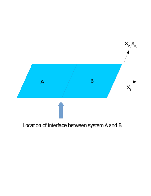
Figure 1: The interface of two subsystems located at $x_{1}=x_{I}$.

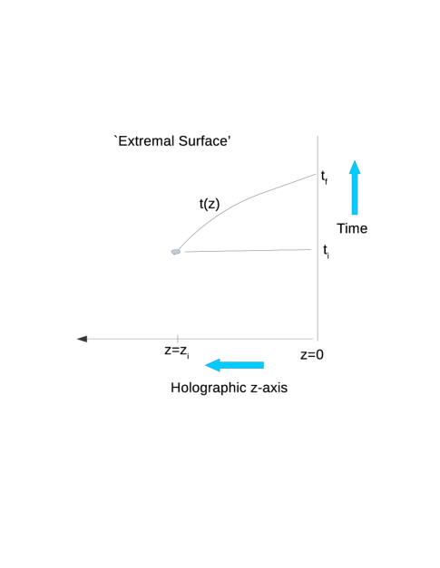
Figure 2: The RT surface between time $t_{i}$ and $t_{f}$. Since $|\partial_{z}x^{0}|\leq 1$ along the extremal curve, we get a cusp-point at $z=z_{i}$.

We are interested in measuring the entanglement information exchange in the CFT staying at the location of interface between two subsystems. The interface divided the whole system into two subsystems and dynamically is a $(d-2)$ dimensional spatial plane, say between system $A$ and the compliment $B$, as shown in figure (1). We intend to calculate the area of a codimension-2 extremal hyper-surfaces embedded in bulk geometry (1) and anchored precisely at the interface, at $x_{1}=x_{I}$, between two large semi-infinite subsystems. Since there is homogeneity and translational invariance, these results will apply to any constant shift in location of the interface ($x_{I}\to x_{I}+a$). (The subsystems in question can be generalized to a strip.)

We now find codimension-2 surface ending at the interface $x_{1}=x_{I}$, and having time-dependent embedding as shown in figure (2). As per holographic prescription [14, 15] generic codimension-2 extremal surfaces can be described by an action functional [16]

$$I \equiv \int{dz\over z^{d-1}}\sqrt{{1\over{f}}+({\partial_{z}x^{1}})^{2}-f(\partial_{z}x^{0})^{2}}$$ (3)

We shall be working only for $d>2$. From eq.(3) it follows that the extremal surfaces satisfy following equations of motion

$${dx^{1}\over dz}\equiv{Pf\over f^{3/2}\sqrt{{E^{2}\over f}-P^{2}+{1\over z^{2d-2}}}}$$

$${dx^{0}\over dz}\equiv{-E\over f^{3/2}\sqrt{{E^{2}\over f}-P^{2}+{1\over z^{2d-2}}}}$$

The parameters ($E,P$) are two integration constants. Since we are interested in knowing the information exchange across the interface, which is a time dependent phenomenon, we will set $x_{1}=constant=x_{I}$ (along with $P=0$). In this way we are selecting purely time-dependent $(d-2)$ dimensional extremal surfaces anchored at the interface $x_{1}=x_{I}$ at the boundary time $x^{0}(0)=t_{f}$. The $t_{f}$ refers to some late time event at the boundary. (In case of the strip we could take $x_{1}=l/2$ as one edge of the strip. The same will be true at the other edge also.) Then equations (2) reduce to a single equation involving time embedding,

$${dx^{0}\over dz}\equiv{-E\over f^{3/2}\sqrt{{E^{2}\over f}+{1\over z^{2d-2}}}}$$

Upon integration (and setting $E\equiv 1/z_{i}^{d-1}$) one obtains

$$\tau\equiv t_{f}-t_{i} \equiv \int_{0}^{z_{i}}dz{(z/z_{i})^{d-1}\over f\sqrt{f+({z/z_{i}})^{2d-2}}}$$

where $t_{i}$ is an initial time event and given by the condition $t_{i}=x^{0}(z)|_{z=z_{i}}$. Through above eq.(2) the constant $z_{i}$ gets related to time interval $\tau$ between two successive events occurring at the interface. To emphasize, since $|x_{0}(z)^{\prime}|\leq 1$, $z=z_{i}$ is at best a cusp-point where the extremal surface starts and it ends at $z=0$, see the figure (2) (It is quite unlike in the HEE nomenclature involving static RT surfaces, there $z_{\ast}$ rather turns out to be the turning point of the RT surface.). Since there is a time translation invariance in the CFT, one may also set $t_{i}=0$ and $t_{f}=\tau$. Thus every where by saying time we shall only mean the time-interval.

Hence the net (entanglement) information exchanged during time interval $\tau$, across $x_{1}=x_{I}$ interface, can be obtained by evaluating the area of extremal surface in (2). From (3)

$$I_{E}={A_{d-2}L^{d-1}\over 4G_{d+1}}\int^{z_{i}}_{\delta}{dz\over z^{d-1}}{1\over\sqrt{f+({z\over z_{i}})^{2d-2}}}$$ (7)

We can note that the information exchanged is dimensionless quantity. The $\delta$ acts as cut-off to regularize UV divergence in the boundary CFT. At $z=z_{i}$ the time coordinate on extremal surface corresponds to the boundary event $(x^{0}(z_{i})=t_{i},x_{1}=x_{I})$. Note $I_{E}$ is proportional to the cross-sectional area of the interface between the subsystems given by $A_{d-2}=l_{2}l_{3}\cdots l_{d-1}$ and it is large. As the integrand becomes singular as we go near to AdS boundary, we would regularize it by the contributions of $x^{0}=constant$, $x^{1}=constant$ surface and single out the divergent piece. Thus we obtain

$$I_{E}|_{x_{1}=x_{I}}= {A_{d-2}L^{d-1}\over 4G_{d+1}}\left(\int^{z_{i}}_{\delta}{dz\over z^{d-1}}({1\over\sqrt{f+({z\over z_{i}})^{2d-2}}}-1)-{1\over(d-2)z_{i}^{d-2}}\right)+I_{UV}$$ (8)

$$={A_{d-2}L^{d-1}\over 4G_{d+1}}{1\over z_{i}^{d-2}}\left(\int^{1}_{0}{d\xi\over\xi^{d-1}}({1\over\sqrt{f+{\xi}^{2d-2}}}-1)-{1\over d-2}\right)+I_{UV}$$

where $\xi\equiv{z\over z_{i}}$, whereas the singular UV contribution is $I_{UV}={A_{d-2}L^{d-1}\over 4G_{d+1}}{1\over(d-2)\delta^{d-2}}$ which is positive definite and diverges. It involves only the area of the interface/boundary. (The UV contribution is thus similar to the entanglement entropy in this aspect, but it is independent of local time information and forms the universal part.) The first term contains all time information and it is finite.

2.1 Stop watch approximation

Let us pick small time interval (say the time period of a stop watch). We wish to measure net information exchanged between two systems staying at the $x_{1}=x_{I}$ interface, and holding a stop watch. For small enough time the extremal surfaces (2) would lie in the vicinity of the asymptotic AdS region only, we can easily expect $z_{i}\ll z_{0}$. In these cases we can evaluate the extremal area (8) perturbatively by expanding it around pure AdS value (i.e. treating pure AdS as a ground state of the CFT). For small $\tau$ values, we first evaluate eq.(2) by making perturbative expansion of the integrand

$$\tau = z_{i}\int_{0}^{1}d\xi\xi^{d-1}{1\over\sqrt{R}}\left(1+{z_{i}^{d}\over z_{0}^{d}}(1+{1\over 2R})\xi^{d}+O(({z_{i}\over z_{0}})^{2d})\right)$$ (9)

$$\equiv z_{i}\left(b_{0}+\epsilon{2b_{1}+i_{11}\over 2}+\cdots\right)$$

where $\xi\equiv{z\over z_{i}}$ and $R(\xi)\equiv 1+\xi^{2d-2}$. The dots indicate terms of higher order in expansion parameter defined as $\epsilon=({z_{i}\over z_{0}})^{d}\ll 1$. The coefficients $b_{0},b_{1}$, and $i_{11}$ are precise integral quantities that are positive definite, but mostly smaller than unity. These numbers are provided in the appendix. The series (9) can also be inverted to obtain the $z_{i}$-expansion

$$z_{i} = \bar{z}_{i}(1-{\bar{z}_{i}^{d}\over z_{0}^{d}}{2b_{1}+i_{11}\over 2b_{0}}+\cdots)$$ (10)

where we define $\bar{z}_{i}={\tau\over b_{0}}$ as the value specific to pure AdS for given interval $\tau$. The equation (10) summarizes the net effect of the metric deformations (with black hole) on the $z_{i}$-value perturbatively. One can easily see that new $z_{i}$ (with excitations) is smaller than $\bar{z}_{i}$ for pure AdS. Having obtained $z_{i}$-expansion, an expansion can now be obtained for the information area functional. From the area integral (8), we get the finite part as

$$I_{E} = {A_{d-2}L^{d-1}\over 4G_{d+1}}{1\over z_{i}^{d-2}}\left(\int_{0}^{1}{d\xi\over\xi^{d-1}}(({1\over\sqrt{R}}-1)+{1\over 2}{z_{i}^{d}\over z_{0}^{d}}{\xi^{d}\over R^{3\over 2}}+\cdots)-{1\over(d-2)}\right)$$ (11)

The respective finite integrals can be separately evaluated at each order to give

$$I_{E} = {A_{d-2}L^{d-1}\over 4G_{d+1}}{1\over z_{i}^{d-2}}(-c_{0}+{z_{i}^{d}\over 2z_{0}^{d}}c_{1}+\cdots)$$

where coefficients $c_{0},c_{1},...$ are precise real values (see the appendix). We emphasize here that $c_{a}$’s are all finite and positive for $d>2$. Substituting $z_{i}$ expression from (10) and keeping terms up to first order we determine

$$I_{E} =I_{UV}-{A_{d-2}L^{d-1}\over 4G_{d+1}}{c_{0}\over\bar{z}_{i}^{d-2}}\left(1+{\bar{z}_{i}^{d}\over z_{0}^{d}}{d-2\over 2}{2b_{1}+i_{11}\over b_{0}}-{\bar{z}_{i}^{d}\over 2z_{0}^{d}}{c_{1}\over c_{0}}\right)+\cdots$$ (13)

$$\equiv I_{AdS}+I_{(1)}$$

while

$$I_{AdS}={A_{d-2}L^{d-1}\over 4G_{d+1}}\left({1\over(d-2)\delta^{d-2}}-{c_{0}b_{0}^{d-2}\over\tau^{d-2}}\right).$$ (14)

is the information exchanged in time $\tau$ for pure $AdS_{d+1}$. It is positive definite and is the leading most term in the expansion. In large time limit $\tau\to\infty$ the $I_{AdS}$ diverges as expected. That is to say an infinite information is exchanged by the subsystems in the CFT ground state. In other words the ground state constitutes maximum to the information mobility. The subsequent term in equation (13)

$$I_{(1)} = {A_{d-2}L^{d-1}\over 4G_{d+1}}{c_{0}\bar{z}_{i}^{2}\over z_{0}^{d}}\left(-(d-2){2b_{1}+i_{11}\over 2b_{0}}+{c_{1}\over 2c_{0}}\right)$$ (15)

consists first order contribution of excitations to the information flow. The information flow remains maximum for pure AdS, as we show next, the first order contribution (due to excitations) is negative and tends to reduce the net information flow. The net change in the information exchange due to excitations is

$$\bigtriangleup I_{E}=-{A_{d-2}L^{d-1}\over 4G_{d+1}}{\tau^{2}D\over b_{0}^{2}z_{0}^{d}}$$ (16)

where $D=\left({-c_{1}\over 2}+(d-2)c_{0}{2b_{1}+i_{11}\over 2b_{0}}\right)>0$. Note coefficient $D$ is positive definite for all $d>2$. Thus the expression on the right hand side of eq.(16) is negative definite, suggesting that the net information exchange for the excited CFT has decreased as compared to the zero temperature CFT. Also it can be noted that $\bigtriangleup I_{E}$ is quadratic in time at first order, suggesting that having black hole excitation in the bulk (or excitations in the CFT) decreases net information flow across the subsystem’s interface.

From eq.(16) we may determine the rate of reduction in information flow relative to the vacuum, as

$${\bigtriangleup I_{E}\over\tau}=-{L^{d-1}A_{d-2}\over 4G_{d+1}}{\tau D\over b_{0}^{2}z_{0}^{d}}<0$$ (17)

The equation (17) represents net loss per unit time in information mobility due to excitations. This remains true at least up to first order. In summarizing, we have learnt that for small time intervals,

• The relative loss in information exchange due to excitations grows quadratically with time.

• The information flow is proportional to cross-section area $A_{d-2}$ of the boundary/interface between the systems.

• It is negative definite for all dimensions indicating that reduction in information flow is an universal feature for excited CFT states.

We will show in the next section that the higher order corrections, as being perturbatively suppressed, cannot change this first order leading behaviour of an excited state. Nevertheless, the absolute sign of second order term will still be important to know here.

2.2 A law of information flow

The physical quantities such as energy or pressure can be obtained by expanding the bulk AdS geometry (1) in Fefferman-Graham asymptotic coordinates suitable near the boundary [17], also in [18]. The energy density of the CFT is given by

$$\bigtriangleup{\cal E}={L^{d-1}\over 16\pi G_{d+1}}{d-1\over z_{0}^{d}}$$

The pressure along all directions is

$$\bigtriangleup{\cal P}={L^{d-1}\over 16\pi G_{d+1}}{1\over z_{0}^{d}}$$ (19)

The eq. (17) in terms of physical observables may also be written as

$${-b_{0}^{2}\bigtriangleup I_{E}\over 4\pi\tau}=\tau A_{d-2}\bigtriangleup{\cal P}_{x_{1}}=\tau\bigtriangleup{\cal F}_{x_{1}}$$ (20)

The negative sign indicates that there is an overall reduction in information flow or mobility and it is directly proportional to the force (pressure) generated by the excitations . However no steady state is reached over small times, as the rate of information loss ${\bigtriangleup\dot{I}_{E}}$ only increases with time initially. However a steady state seems to have been reached after long times, where our perturbative approach would rather fail. The numerical plots in figures (4), (6), (8) suggest that late time behaviour generically

$$Lim_{\tau\to\infty}\bigtriangleup I_{E}\to 0$$ (21)

The above limit may lead to finite answer too. Especially in 2-dimensional case the late time behaviour can be exactly determined. We discuss it in the subsection.

The equation (20) short of mimics flow of charge in a conductor under the effect of external emf (force). In the entanglement context here the eq.(20) thus describes a law of information flow over small time interval. The negative sign is crucial and universal feature for all $d$. We may recall that the entanglement entropy usually rises whenever CFT has excitations [18]. This growth in HEE may appear to be related to loss in information exchange between the subsystems. Nevertheless it is clear that CFT pressure plays vital role in (entanglement) information exchange (flow).

2.3 Information at second order and a bound

In order to make this more robust we need to calculate higher order terms. Taking steps as in the previous section, we calculate the second order terms in the expansion of the information integral, which we schematically denote as

$$I\equiv I_{AdS}+I_{(1)}+I_{(2)}+\cdots$$ (22)

where $I_{AdS}$ and first order term $I_{(1)}$ have already been obtained. We focus on finding $I_{(2)}$ and its absolute sign in the next. In the first step, we obtain expansion for $z_{i}$ in terms of $\tau$, as done in (9) and (10), up to second order

$$z_{i} = \bar{z}_{i}\big{[}1-{(2b_{1}+i_{11})\over 2b_{0}}\bar{\epsilon}+{8b_{1}^{2}(d+1)+8b_{1}(d+1)i_{11}+2(d+1)i_{11}^{2}\over 8b_{0}^{2}}\bar{\epsilon}^{2}$$ (23)

$$- {b_{0}(8b_{2}+4i_{21}+3i_{22})\over 8b_{0}^{2}}\bar{\epsilon}^{2}+O(\bar{\epsilon}^{3})\big{]}$$

where $\bar{\epsilon}\equiv{\bar{z}_{i}^{d}\over z_{0}^{d}}\ll 1$ is the expansion parameter. In the next step the extremal area calculation leads to the following second order term

$$I_{(2)} = {L^{d-1}A_{d-2}\over 4G_{d+1}}{1\over\bar{z}_{i}^{d-2}}[{3c_{2}\over 8}+(d-2){c_{1}(2b_{1}+i_{11})\over 4b_{0}}$$ (24)

$$-{c_{1}d(2b_{1}+i_{11})\over 4b_{0}}-{c_{0}\over 8b_{0}^{2}}(d-2)(-12b_{1}^{2}+8b_{0}b_{2}-4b_{1}^{2}d-12b_{1}i_{11}$$

$$-4b_{1}di_{11}-3i_{11}^{2}-di_{11}^{2}+4b_{0}i_{21}+3b_{0}i_{22})]\bar{\epsilon}^{2}$$

The parameters $b_{a},~{}i_{ab}$ and $c_{a}$ have definite numerical values provided in the appendix. It is not important to know them all. A significant result follows from here is that, the $I_{(2)}$ is positive definite for all $d>2$. This has been thoroughly checked by us. The absolute sign of second order term is important as this will provide us with a bound. It leads to an immediate conclusion that the loss in information exchange will have a bound, namely

$$b_{0}^{2}{|\bigtriangleup I_{E}|\over 4\pi\tau^{2}}\leq\bigtriangleup{\cal F}_{x_{1}}$$ (25)

where the net force ${\cal F}_{x_{1}}$ is given by cross-section area of the interface times the entanglement pressure ${\cal P}_{x_{1}}$ along the $x_{1}$ direction. The force is in the transverse direction of the interface between subsystems.

To proceed further we now study individual case of $CFT_{d}$. Let us discuss phenomena for $d=3,4,6$ only to gain some insight.

Case-I: for $d=4$ $(AdS_{5})$

The relative information flow per unit area per unit time up to second order is obtained as

$$-{b_{0}^{2}\bigtriangleup I_{E}\over A_{2}\tau}=4\pi\alpha_{4}\tau\left(1-{.902\over\alpha_{4}}({\tau\over b_{0}z_{0}})^{4}+{2.676\over\alpha_{4}}({\tau\over b_{0}z_{0}})^{8}+O(\bar{\epsilon}^{3})\right)\bigtriangleup P_{x_{1}}$$ (26)

where numerical values of some coefficients for the purpose of estimate are as $\alpha_{4}\simeq 0.558,~{}b_{0}\simeq.215$. The $x_{1}$ component of $CFT$ pressure exerted on the interface located at $x_{1}=x_{I}$, is $\bigtriangleup P_{x_{1}}={L^{3}\over 16\pi G_{5}}{1\over z_{0}^{4}}$ while area of boundary is $A_{2}$. It is remarkable that the equation (26) is in the factorized form and may be written as

$$-{b_{0}^{2}\bigtriangleup I_{E}\over A_{2}\tau}={4\pi\alpha_{4}}\tau Q(t,z_{0})\bigtriangleup P_{x_{1}}$$ (27)

where the factor $Q$ is

$$Q=\left(1-{.902\over.558}({\tau\over b_{0}z_{0}})^{4}+O(\bar{\epsilon}^{2})\right)$$ (28)

and it is always smaller than unity. It may be an indication that effectively the time period (or time per collision) gets shortened after inclusion of higher order terms in the perturbative expansion. An explicit negative sign on the lhs indicates that there is overall reduction in the information flow for the excited states. As the case here the CFT excitations are thermal, but actually that need not have been the case. The results would be identical for all finite energy (IR) gravity perturbations in the bulk.

However we may define the quantum information decay rate per unit area as

$$-{b_{0}^{2}\bigtriangleup I_{E}\over A_{2}\tau} = 4\pi\alpha_{4}Q(\tau)\tau\bigtriangleup P_{x_{1}}$$ (29)

$$\simeq {4\pi\alpha_{4}\over d-1}Q(\tau)\tau\bigtriangleup{\cal E}$$

$$\leq {2\pi\alpha_{4}\over d-1}$$

The last inequality follows because $0<Q<1$, and for a quantum state with energy $\bigtriangleup{\cal E}$ and a half-life $\tau$ it is understood that $\tau\bigtriangleup{\cal E}\simeq{1\over 2}$ due to the uncertainty.

Case-2: for $d=3$ This case involves a 3-dimensional boundary theory which is dual of $AdS_{4}$. The spacetime $AdS_{4}$ arises as near horizon geometry of multiple M2-branes in $11$-dimensional supergravity. The subsystem interface here is 1-dimensional. It is found that

$$-{b_{0}^{2}\bigtriangleup I_{E}\over A_{1}\tau}=4\pi\alpha_{3}\tau\left(1-{.631\over\alpha_{3}}({\tau\over b_{0}z_{0}})^{3}+{1.328\over\alpha_{3}}({\tau\over b_{0}z_{0}})^{6}+O(\bar{\epsilon}^{3})\right)\bigtriangleup P_{x_{1}}$$ (30)

where we have used numerical values, $\alpha_{3}\approx 0.528,~{}b_{0}\simeq.284$. The component of $CFT_{3}$ pressure $\bigtriangleup P_{x_{1}}={L^{2}\over 16\pi G_{4}z_{0}^{3}}$ exerted on the subsystem boundary located at $x_{1}=x_{I}$, wheras $A_{1}$ is length of the interface.

Case-3: for $d=6$ The information flow per unit area per unit time up to second order for $AdS_{7}$ bulk spacetime is given by

$$-{b_{0}^{2}\bigtriangleup I_{E}\over A_{4}\tau}=4\pi\alpha_{6}\tau\left(1-{1.457\over\alpha_{6}}({\tau\over b_{0}z_{0}})^{6}+{6.821\over\alpha_{6}}({\tau\over b_{0}z_{0}})^{12}+O(\bar{\epsilon}^{3})\right)\bigtriangleup P_{x_{1}}$$ (31)

where we have $\alpha_{6}\simeq 0.588,~{}b_{0}\simeq.144$. The component of $CFT_{6}$ pressure $\bigtriangleup P_{x_{1}}={L^{5}\over 16\pi G_{7}}{1\over z_{0}^{6}}$ exerted on the system boundary located at $x_{1}=x_{I}$, while 4-dimensional subsystem interface area is $A_{4}$.

3 Special case of $AdS_{3}$

The $AdS_{3}$ case is special where boundary CFT is 2-dimensional and bulk geometry is the BTZ black hole. The subsystem interface or junction is just point-like or a dot. From (2) we get the slope of the $x^{0}$ extremal surface at the cusp point as

$${t^{\prime}}|_{z=z_{i}}={1\over(1-{z_{i}^{2}\over z_{0}^{2}})\sqrt{2-{z_{i}^{2}\over z_{0}^{2}}}}\geq{1\over\sqrt{2}}$$ (32)

that is bounded by its lowest value ${1\over\sqrt{2}}$ for pure $AdS_{3}$. Upon inegration the exact expression for the cusp value $z_{i}$ in terms of time gap $\tau$, by integrating (2), becomes

$$\tanh({\tau\over z_{0}})={{z_{i}\over z_{0}}(\sqrt{2-{z_{i}^{2}\over z_{0}^{2}}}-1)\over 1-{z_{i}^{2}\over z_{0}^{2}}\sqrt{2-{z_{i}^{2}\over z_{0}^{2}}}}$$ (33)

A plot for $\tau~{}Vs~{}z_{i}$ has been provided in the figure (3).

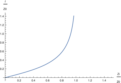
Figure 3: The $\tau~{}Vs~{}z_{i}$ plot for BTZ case. When $z_{i}/z_{0}\to 1$ the net time required for information processing becomes very large indeed. We have taken $z_{0}=1$ here.

Finally the net information processsed by a quantum dot from eq. (7) is

$$I_{E}={L\over 4G_{3}}\left(\ln\left({z_{i}\over\bar{z}_{i}}{1\over 1+\sqrt{2-{z_{i}^{2}\over z_{0}^{2}}}}\right)+\ln{2\bar{z}_{i}\over\delta}\right)$$ (34)

whereas $\bar{z}_{i}={\tau\over b_{0}}$ is the value corresponding to pure $AdS_{3}$ (Note here $b_{0}=\sqrt{2}-1$). For the pure $AdS_{3}$ (i.e. $CFT_{2}$ ground state) the net information processed in given time interval is given by

$$I_{AdS_{3}}={L\over 4G_{3}}\ln({2\tau\over b_{0}\delta}).$$ (35)

These are exact expressions.

For large time ($\tau\to\infty$ ) we find from (34) that

$$Lim_{t\to\infty}I_{E}={L\over 4G_{3}}\ln({z_{0}\over\delta})>0.$$ (36)

This expression is finite and completely independent of the time. The small variations follow a relation

$$\delta I_{E}\simeq-{L\over 4G_{3}}{z_{0}^{2}\over 2}\delta\left({1\over z_{0}^{2}}\right)=-{8\over\pi T_{th}^{2}}\delta{\cal M}$$ (37)

where ${\cal M}$ is the energy density of the BTZ black hole and $T_{th}\sim{2\over\pi z_{0}}$ is horizon temperature. It can seen that all local time dependence disappears or wiped out after large intervals. This large time limit (37) may be recasted purely in terms of thermal entropy density as

$$\delta I_{E}+{8\over\pi T_{th}}\delta s_{th}=0$$ (38)

It is an exact relation for the information processed by a quantum dot (at the interface of the subsystem) and corresponding rise in the entropy of any excited state of the system. Note here the CFT is 1-dimensional (spatial) and the system interface is thus point-like. It suggests that the rise in thermal entropy is always detrimental to the information flow (or processing), read conductivity, and vice versa.

4 Numerical results

In the previous section we could make perturbative study of the information flow for finite times only. However the results at large times were elusive because the perturbation breaks down. To understand the late time behaviour of information exchange we pick three cases of $AdS_{4}$, $AdS_{5}$ and $AdS_{6}$.

For $d=3$ the two plots are obtained in figures (4) and (5).

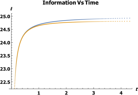
Figure 4: Net information exchange per unit area of the interface as a function of time for $d=3$ case. We have taken $I_{UV}=25,~{}z_{0}=5,~{}L=1,~{}G_{N}=1/4$. The upper curve represents $I_{AdS_{4}}$. It shows maximum information is exchanged in the ground state.

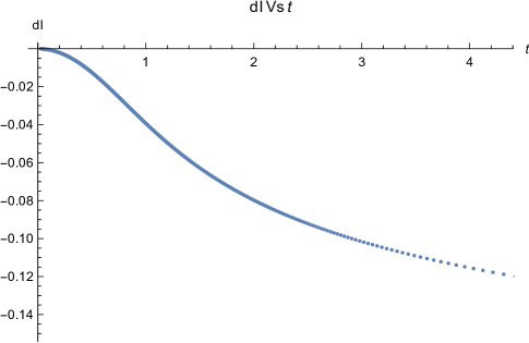
Figure 5: The loss in information flow with excitations for $d=3$. We have taken $I_{UV}=25,~{}z_{0}=5$.

In the fig.(4) the net information exchange for excited $CFT_{3}$ rises sharply in tandem with ground state growth and actually grows very close up to the ground state plot. But at late time the two growths differ considerably. The difference of growth $\bigtriangleup I$ is plotted in the figure (5). It depicts a net reduction in the entanglement growth for the excited state. The information loss initially grows quadratically in time and then slows down at late times. The similar results for $CFT_{4}$ are given in figure (6) and (7).

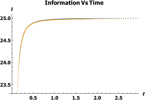
Figure 6: Net information exchange per unit area of the interface as a function of time for $d=4$ case. We have taken $I_{UV}=25,~{}z_{0}=5,~{}L=1,~{}G_{N}=1/4$. The upper curve represents $I_{AdS_{5}}$. It shows maximum information is exchanged in the ground state only.

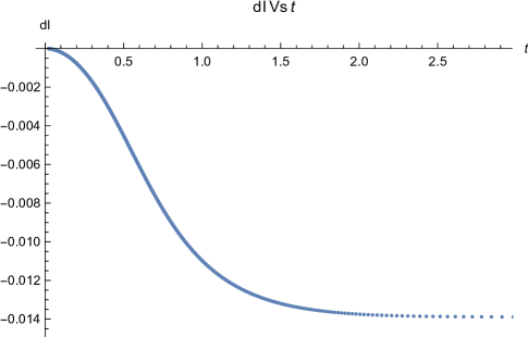
Figure 7: The loss in information flow with excitations for $d=4$. We have set $I_{UV}=25,~{}z_{0}=5$.

These graphs show universal feature that information loss (with excitations) grows quadratically near $t=0$, but it appears to get saturated at late times and curve gets flattened. These results for excited states of $CFT_{5}$ can be found in figs.(8) and (9). There too the information loss curve behaves quadratically in time initially but unlike previous two cases it rebounds and information loss starts reducing at late times. This is a direct effect of dimensionality of the theory. The early time behaviour is consistent with perturbative analysis where first order term is indeed quadratic in time.

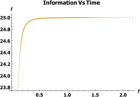
Figure 8: Net information exchange per unit area of the interface as a function of time for $d=5$ case. We have taken $I_{UV}=25,~{}z_{0}=5,~{}L=1,~{}G_{N}=1/4$. The upper curve represents $I_{AdS_{6}}$. It shows maximum information is exchanged in the ground state.

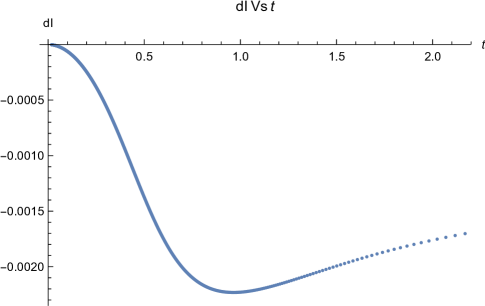
Figure 9: The loss in information flow with excitations for $d=5$. We have taken $I_{UV}=25,~{}z_{0}=5$.

5 Quantum Complexity

We now evaluate another time dependent quantity when the CFT is in excited state. The complexity of quantum circuits is a measure of time evolution of the state of the system as a whole. It can be defined holographically by the volume action functional describing a time-dependent (codim-1) extremal surface [7]

$$C_{E} \equiv {V_{d-1}L^{d}\over 4G_{d+1}}\int{dz\over z^{d}}\sqrt{{f}^{-1}-f(\partial_{z}x^{0})^{2}}$$ (39)

where $V_{d-1}\equiv l_{1}l_{2}l_{3}\cdots l_{d-1}$ is the net spatial volume of the CFT. In this sense quantum complexity is a bulk property of the CFT and extensive in nature. Note the difference that the volume complexity is dimensionful whereas information exchange $I_{E}$ is dimensionless. From (39) it follows that extremal surfaces have to satisfy following equation of motion

$${dx^{0}\over dz}\equiv{z^{d}/z_{c}^{d}\over f\sqrt{f+z^{2d}/z_{c}^{2d}}}$$

The $z_{c}$ is the integration constant and it will get related to the time interval on the boundary. To first solve $x^{0}$ equation, let us choose an extremal surface having boundary value $x^{0}(0)=t_{f}$, where $t_{f}$ is a time event on the boundary. The eq.(5) gives upon integrating

$$\tau=t_{f}-t_{i} \equiv \int_{0}^{z_{c}}dz{(z/z_{c})^{d}\over f\sqrt{f+({z/z_{c}})^{2d}}}$$

where $t_{i}$ is some initial time given by $t_{i}=x^{0}|_{z=z_{c}}$. Thus the constant $z_{c}$ gets related to time interval between two events on the boundary. There is overall time translation invariance in the system. It is also clear that for small intervals we will have a situation where $z_{c}\ll z_{0}$.

The expression for complexity during time interval $\tau$, can be obtained by calculating the area of the extremal surface from action (39)

$$C_{E}={V_{d-1}L^{d}\over 4G_{d+1}}\int^{z_{c}}_{\delta}{dz\over z^{d}}{1\over\sqrt{f+({z\over z_{c}})^{2d}}}$$ (42)

The integrand in (42) becomes singular near the AdS boundary which is the UV divergence of the CFT. We can regularize it by the contribution of $x^{0}=constant$ surface and single out the diverging UV part. Thus we obtain

$$C_{E}={V_{d-1}L^{d}\over 4G_{d+1}}{1\over z_{c}^{d-1}}\left(\int^{1}_{0}{d\xi\over\xi^{d}}({1\over\sqrt{f+{\xi}^{2d}}}-1)-{1\over d-1}\right)+C_{UV}$$ (43)

The divergent part is given by $C_{UV}={V_{d-1}L^{d}\over 4G_{d+1}}{1\over(d-1)\delta^{d-1}}$, it is positive definite and proportional to spatial volume of the CFT. We will now evaluate $C_{E}$ perturbatively for small $\tau$. First, by evaluating rhs of eq.(5) up to first order, we find

$$z_{c}=\bar{z}_{c}(1-{2f_{1}+j_{1}\over 2f_{0}}\bar{\epsilon}+O(\epsilon^{2}))$$ (44)

where $\bar{z}_{c}={\tau\over f_{0}}$ and expansion parameter $\bar{\epsilon}={\bar{z}_{c}^{d}\over z_{0}^{d}}\ll 1$. The coefficients $f_{0},~{}f_{1}$ and $j_{1}$ are all finite and given in the appendix. It is not immediately important to know them here. Using $z_{c}$ equation (44) and substituting in (43), we find the net change in complexity $(C_{E}-C_{AdS})$ to be given as

$$\bigtriangleup C_{E} = {V_{d-1}L^{d}\over 4G_{d+1}}{d_{0}\bar{z}_{c}\over z_{0}^{d}}\left(-(d-1){2f_{1}+j_{1}\over 2f_{0}}+{d_{1}\over 2d_{0}}\right)+higher~{}orders$$ (45)

$$=-{V_{d-1}L^{d}\over 4G_{d+1}}{\tau\over f_{0}}{D_{c}\over z_{0}^{d}}+higher~{}orders$$

Thus up to first order the change in complexity per unit volume per unit time is

$${f_{0}\bigtriangleup C_{E}\over V_{d-1}\tau} \simeq -{4\pi D_{c}}\bigtriangleup{\cal{E}}$$ (46)

where

$$D_{c}\equiv(d-1)d_{0}{2f_{1}+j_{1}\over 2f_{0}}-{d_{1}\over 2}$$

and note that $D_{c}>0$ for all $d$ values. For example, for $d=4$ one gets $D_{c}\approx.432$ and $f_{0}\simeq.173$. Thus the negative sign in (46) indicates that overall holographic complexity (HC) of the excited CFT will get reduced as compared to the ground state (i.e. pure AdS). This reduction in circuit complexity is analogous to the reduction in information exchange at the interface in previous section. While, in contrast, we may recall here that entanglement entropy (HEE) increases when the CFT is excited. We interpret the two opposing natures of HC and HEE, by suggesting that complexity is a measure of (global) symmetries of a given quantum state. The complexity will get reduced with increased symmetry of a quantum state. But excitations are also cause of rise in the (internal) disorder in the system, whence the HEE will essentially increase. But amidst disorder there can still be an overall enhancement of the global symmetry in the system (such as rotations), and therefore the HC would decrease. It is very much like the phenomena we encounter in ferro-magnetic (spin) systems in three dimensions.

5.1 A bound on loss of information exchange

The bound in the last section on relative information flow can also be stated differently in terms of complexity as (in $d>2$)

$${b_{0}^{2}\bigtriangleup\dot{I}_{E}\over A_{d-2}}\leq{2\alpha_{d}\over LD_{c}}{f_{0}\bigtriangleup C_{E}\over V_{d-1}}$$ (47)

where $A_{d-2}$ is the area of the system’s interface and $V_{d-1}$ is total volume of the system. $\bigtriangleup C_{E}$ measures the net loss in quantum complexity. The constants $\alpha_{d}$ and $D_{c}$ depend on spacetime dimensions. (Especially for $d=4$, we have $\alpha_{4}\simeq.558$ and $D_{c}\simeq.432$.) The inequality (47) can be obtained for any excited CFT state. It states that rate of loss in information flow due to the excitations remains bounded by the corresponding loss in the quantum complexity of the given state. However, as we notice both quantities suffer loss in the presence of the excitations. The excitations in the present case are thermal due to the black holes in the bulk. But the above relation would remain true for any positive energy fluctuations also.

6 Summary

We explored net quantum information exchange or sharing in real time at the interface between subsystems for $CFT_{d}$ living at the boundary of $AdS_{d+1}$ spacetimes. The information exchange is a continuous phenomenon and only after long time intervals full information exchange gets saturated. Generally we prepare systems for small time intervals only. We find perturbatively that the rate of information exchange between two systems is always reduced when the systems have excitations for all $d$, while CFT ground state has a maximum information exchange rate. The net information loss is directly proportional to the force or pressure generated by the CFT excitations. We get a bound

$$b_{0}^{2}{|\bigtriangleup I_{E}|\over 4\pi\tau^{2}}\leq\bigtriangleup{\cal F}_{x_{1}}$$

where the force ${\cal F}_{x_{1}}$ is in transverse direction to the interface. The inequality is saturated only at the first order of perturbation. Especially for 2-dimensional CFT, the large time relation can be recasted in terms of thermal entropy density as

$$\delta I_{E}+{8\over\pi T_{th}}\delta s_{th}=0$$

It is an exact relation for the loss in information processed by the quantum dot (the interface) and corresponding rise in thermal entropy for the excited state of the system. Note the $CFT_{2}$ system represents 1-dimensional wire and the subsystem interface is only point-like. It proves that the rise in entropy is always detrimental to the information flow (or conductivity) and vice versa.

We further observed that there is an overall reduction in quantum complexity too in the presence of excitations. While it is well understood that excited states add more to the entanglement entropy due to rise in disorder. From this perspective we are led to argue that the reduction in the complexity may be due to relative higher symmetry excited states may have as compared to CFT ground state. The ground state is always more ordered but it maybe less symmetric as we observe in ferromagnetic systems with an spontaneously broken symmetry.

We have got a new bound which states that rate of loss in the information flow due to excitations will remain bounded by the corresponding loss in quantum complexity for a given state of the system.

Before we conclude there are a few clarifications to add. Most of our computations are on the gravity side assuming standard holographic method. It would be challenging to develop same perspective on the boundary side. We have observed that information exchange is generally reduced in the presence of excitations in the CFT as compared to the ground state (at zero temperature). This is found to be true in all dimensions. The reduction in information exchange is also one of the common characterisitic in most systems (classical or quantum) found in nature. As an example the transport in metals (a type of information flow) is also reduced at high temperatures and in the presence of impurities too. It would be interesting to understand the information processing of quantum computers in real time which work on the principle of quantum teleporation. The quantum-dot in section-3 is an interface or junction of 1-dimensional wire like system and it works quite like a quantum computer. It processes the information lying on two sides of the wire. Furthermore, we have only considered black holes as excitations on top of pure AdS geometry. This was for simplicity purposes only. However the calculations are mostly perturbative and results depend upon dimensionless ratio, $z_{i}/z_{0}$, which is very small than unity. So we are studying boundary phenomena over small time intervals for which the extremal surfaces reside in the asymptotic region only. The actual black hole (IR) geometry does not play significant role in it. This indicates that other small excitations of the AdS geometry can also be studied and we believe the outcome would be similar.

Appendix A Integral Quantities

Some useful integral values we have used in the calculation of information flow are being noted down here (where $R(\xi)=1+\xi^{2d-2}$)

$$b_{0}=\int_{0}^{1}d\xi\xi^{d-1}{1\over\sqrt{R}}\simeq.284~{}({\rm for}~{}d=3)$$

$$b_{1}=\int_{0}^{1}d\xi\xi^{2d-1}{1\over\sqrt{R}}\simeq.133~{}({\rm for}~{}d=3)$$

$$b_{2}=\int_{0}^{1}d\xi\xi^{3d-1}{1\over\sqrt{R}}\simeq.086~{}({\rm for}~{}d=3)$$

$$i_{11}=\int_{0}^{1}d\xi\xi^{2d-1}{1\over R\sqrt{R}}\simeq.087~{}({\rm for}~{}d=3)$$

$$i_{21}=\int_{0}^{1}d\xi\xi^{3d-1}{1\over R\sqrt{R}}\simeq.052~{}({\rm for}~{}d=3)$$

$$i_{22}=\int_{0}^{1}d\xi\xi^{3d-1}{1\over R^{2}\sqrt{R}}\simeq.033~{}({\rm for}~{}d=3)$$

$$c_{0}=\int_{0}^{1}d\xi\xi^{1-d}(1-{1\over\sqrt{R}})+{1\over d-2}\simeq 1.131~{}({\rm for}~{}d=3)$$

$$c_{1}=\int_{0}^{1}d\xi{\xi\over R\sqrt{R}}\simeq.353~{}({\rm for}~{}d=3)$$

$$c_{2}=\int_{0}^{1}d\xi{\xi^{d+1}\over R^{2}\sqrt{R}}\simeq.077~{}({\rm for}~{}d=3),$$ (48)

We have provided numeric values for $d=3$ case only. For other $d$ cases one can obtain these values easily.

Another set of integral coefficients which appear in complexity are (with $R(\xi)=1+\xi^{2d}$)

$$f_{0}=\int_{0}^{1}d\xi\xi^{d}{1\over\sqrt{R}}\simeq.214~{}({\rm for}~{}d=3)$$

$$f_{1}=\int_{0}^{1}d\xi\xi^{2d}{1\over\sqrt{R}}\simeq.117~{}({\rm for}~{}d=3)$$

$$j_{1}=\int_{0}^{1}d\xi\xi^{2d}{1\over R\sqrt{R}}\simeq.080~{}({\rm for}~{}d=3)$$

$$d_{0}=\int_{0}^{1}d\xi\xi^{-d}(1-{1\over\sqrt{R}})+{1\over d-1}\simeq 0.599~{}({\rm for}~{}d=3)$$

$$d_{1}=\int_{0}^{1}d\xi{1\over R\sqrt{R}}\simeq 0.867~{}({\rm for}~{}d=3)$$

while

$$f_{0}=\int_{0}^{1}d\xi\xi^{d}{1\over\sqrt{R}}\simeq.173~{}({\rm for}~{}d=4)$$

$$f_{1}=\int_{0}^{1}d\xi\xi^{2d}{1\over\sqrt{R}}\simeq.091~{}({\rm for}~{}d=4)$$

$$j_{1}=\int_{0}^{1}d\xi\xi^{2d}{1\over R\sqrt{R}}\simeq.063~{}({\rm for}~{}d=4)$$

$$d_{0}=\int_{0}^{1}d\xi\xi^{-d}(1-{1\over\sqrt{R}})+{1\over d-1}\simeq 0.413~{}({\rm for}~{}d=4)$$

$$d_{1}=\int_{0}^{1}d\xi{1\over R\sqrt{R}}\simeq 0.107~{}({\rm for}~{}d=4)$$

We have only provided these numerical values just for having an idea.

References

- [1] J. Maldacena, Adv. Theor. Math. Phys. 2, 231 (1998) arXiv:9711200[hep-th]; S. Gubser, I. Klebanov and A.M. Polyakov, Phys. lett. B 428, 105 (1998) arXiv:9802109[hep-th]; E. Witten, Adv. Theor. Math. Phys. 2, 253 (1998) arXiv:9802150[hep-th].
- [2] A.K. Pati and S.L. Braunstein, NATURE 404, 164 (2000); S.L. Braunstein and A.K. Pati, Phys. Rev. Lett. 98, 080502 (2007);
- [3] J. R. Samal, A. K. Pati, and Anil Kumar, Phys. Rev. Lett. 106, 080401 (2011).
- [4] D. N. Page, Average entropy of a subsystem, Phys. Rev. Lett.71 (1993) 1291–1294, [gr-qc/9305007].
- [5] G. Penington, S. H. Shenker, D. Stanford and Z. Yang, “Replica wormholes and the black hole interior”, arXiv:1911.11977[hep-th]; A. Almheiri, R. Mahajan and J. Maldacena, “Islands outside the horizon”, arXiv:1910.11077[hep-th]; A. Almheiri, T. Hartman, J. Maldacena, E. Shaghoulian and A. Tajdini, “Replica Wormholes and the Entropy of Hawking Radiation”, JHEP05 (2020) 013, arXiv:1911.12333.
- [6] Suvrat Raju, “Lessons from the Information Paradox”, arXiv:2012.05770.
- [7] L. Susskind, arXiv:1810.11563[hep-th]; Fortschr. Phys. 64 (2016) 24; D. Stanford and L. Susskind, Phys. Rev. D90 (2014) 126007.
- [8] A.R. Brown , D.A. Robert, L. Susskind, B. Swingle, and Y. Zhao, Phys. Rev. Lett 116 (2016) 191301; A.R. Brown , D.A. Robert, L. Susskind, B. Swingle, and Y. Zhao, Phys. Rev. Lett 93 (2016) 086006;
- [9] A. Bernamonti et.al, Phys. Rev. Lett. 123 (2019) 081601.
- [10] A. Bhattacharyya, P. Caputa, S.R. Das, N. Kundu, M. Miyaji, and T. Takayanagi, JHEP 07 (2018) 086; P. Caputa, N. Kundu, M. Miyaji, T. Takayanagi, and K. Watanbe, Phys. Rev. Lett. 119 (2017) 071602; P. Caputa, N. Kundu, M. Miyaji, T. Takayanagi, and K. Watanbe, JHEP112017097;
- [11] K. Hashimoto, N. Iizuka, and S. Sugishita, Phys. Rev D96 (2017) 126001; K. Hashimoto, N. Iizuka, and S. Sugishita, arXiv:1805.04226[hep-th]
- [12] D. Carmi, S. Chapman, H. Marrochio, R. Myers, and S. Sugishita, arXiv:1709.10184[hep-th].
- [13] G. Di Giulio and E. Tonni, “Complexity of mixed Gaussian states from Fisher information geometry,” JHEP 12 (2020), 101 [arXiv:2006.00921 [hep-th]].
- [14] S. Ryu and T. Takayanagi, Phys. Rev. Lett. 86 (2006) 181602, arXiv:0603001[hep-th]; S. Ryu and T. Takayanagi, JHEP 0608 (2006) 045, arXiv:0605073[hep-th].
- [15] V. E. Hubeny, M. Rangamani and T. Takayanagi, JHEP 0707 (2007) 062, arXiv: 0705.0016 [hep-th].
- [16] R. Bousso, H. Casini, Z. Fisher, and J. Maldacena, Phys. Rev. D 91, 084030 (2015) ,arXiv:1406.4545[hep-th].
- [17] V. Balasubramanian and P. Kraus, Commun. Math. Phys. 208, 413 (1999) [hep-th/9902121]; P. Kraus, F. Larsen and R. Siebelink, Nucl. Phys. B 563, 259 (1999) [hep-th/9906127]; M. Bianchi, D. Z. Freedman and K. Skenderis, Nucl. Phys. B 631, 159 (2002) [hep-th/0112119].
- [18] R. Mishra and H. Singh, JHEP 10 (2015), 129 [arXiv:1507.03836 [hep-th]].
- [19] A. Ramesh Chandra, J. de Boer, M. Flory, M. P. Heller, S. Hörtner and A. Rolph Spacetime as a quantum circuit , arXiv:2101.01185[hep-th].