The joint role of geometry and illumination on material recognition

Abstract.

Observing and recognizing materials is a fundamental part of our daily life. Under typical viewing conditions, we are capable of effortlessly identifying the objects that surround us and recognizing the materials they are made of. Nevertheless, understanding the underlying perceptual processes that take place to accurately discern the visual properties of an object is a long-standing problem. In this work, we perform a comprehensive and systematic analysis of how the interplay of geometry, illumination, and their spatial frequencies affects human performance on material recognition tasks. We carry out large-scale behavioral experiments where participants are asked to recognize different reference materials among a pool of candidate samples. In the different experiments, we carefully sample the information in the frequency domain of the stimuli. From our analysis, we find significant first-order interactions between the geometry and the illumination, of both the reference and the candidates. In addition, we observe that simple image statistics and higher-order image histograms do not correlate with human performance. Therefore, we perform a high-level comparison of highly non-linear statistics by training a deep neural network on material recognition tasks. Our results show that such models can accurately classify materials, which suggests that they are capable of defining a meaningful representation of material appearance from labeled proximal image data. Last, we find preliminary evidence that these highly non-linear models and humans may use similar high-level factors for material recognition tasks.

1. Introduction

Under typical viewing conditions, humans are capable of effortlessly recognizing materials and inferring many of their key physical properties, just by briefly looking at them. While this is almost an effortless process, it is not a trivial task. The image that is input to our visual system results from a complex combination of the surface geometry, the reflectance of the material, the distribution of lights in the environment, and the observer’s point of view. To recognize the material of a surface while being invariant to other factors of the scene, our visual system carries out an underlying perceptual process that is not yet fully understood [Dror et al., 2001a; Fleming et al., 2001; Adelson, 2000].

So how does our brain recognize materials? We could think that, similar to solving an inverse optics problem, our brain is estimating the physical properties of each material [Pizlo, 2001]. This would imply knowledge of many other physical quantities about the object and its surrounding scene, from which our brain could disentangle the reflectance of the surface. However, we rarely have access to such precise information, so variations based on Bayesian inference have been proposed [Kersten et al., 2004].

Other approaches are based on image statistics, and explain material recognition as a process where our brain extracts image features that are relevant to describe materials. Then, it would try to match them with previously acquired knowledge, in order to discern the material we are observing. Considering this approach our visual system would disregard the illumination, motion, or other factors in the scene and try to recognize materials by representing their typical appearance in terms of features instead of explicitly acquiring an accurate physical description of each factor. This type of image analysis can be carried out in the primary domain [Geisler, 2008; Adelson, 2008; Fleming, 2014; Motoyoshi et al., 2007; Nishida and Shinya, 1998], or in the frequency domain [Oliva and Torralba, 2001; Brady and Oliva, 2012; Giesel and Zaidi, 2013]. However, it is argued if our visual system actually derives any aspects of material perception from such simple statistics [Anderson and Kim, 2009]. For instance, Fleming and Storrs [2019] have recently proposed the idea that highly non-linear encodings of the visual input may better explain the underlying processes of material perception.

In this work, we thoroughly analyze how the confounding effects of illumination and geometry influence human performance in material recognition tasks. The same material can yield different appearances due to changes in illumination and/or geometry (see Figures 1 and 2), while it is possible to have two different materials look the same by tweaking the two parameters [Vangorp et al., 2007].

Figure 1. Two spheres made of silver, under two different illuminations, leading to completely different pixel-level statistics.

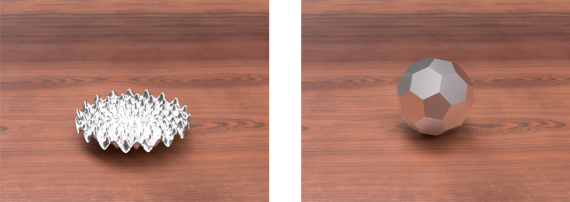
Figure 2. Two objects of different geometries but made of the same material, under the same illumination. The object on the left appears to be made of a shinier material.

We aim to further our understanding of the complex interplay between geometry and illumination in material recognition. We have carried out large-scale, rigorous online behavioral experiments where participants were asked to recognize different materials, given images of one reference material and a pool of candidates. By using photorealistic computer graphics, we obtain carefully controlled stimuli, with varying degrees of information in the frequency domain. In addition, we observe that simple image statistics, image histograms, and histograms of V1-like subband filters do not correlate with human performance in material recognition tasks. Inspired by Fleming and Storrs’ recent work [2019], we analyze highly non-linear statistics by training a deep neural network. We observe that such statistics define a robust and accurate representation of material appearance and find preliminary evidence that these models and humans may share similar high-level factors when recognizing materials.

1.1. Material recognition

Recognizing materials and inferring their key features by sight is invaluable for many tasks. Our experience suggests that humans are able to correctly predict a wide variety of rough material categories like textiles, stones, or metals [Fleming, 2014; Ged et al., 2010; Fleming and Bülthoff, 2005; Li and Fritz, 2012]; or items that we would call ”stuff” [Adelson, 2001] — like sand or snow—. Humans are also capable of identifying the materials in a photograph by briefly looking at them [Sharan et al., 2009, 2008] or of inferring their physical properties without the need to touch them [Fleming et al., 2013, 2015a; Maloney and Brainard, 2010; Nagai et al., 2015; Serrano et al., 2016; Jarabo et al., 2014]. This ability is built from experience, by actually confirming visual impressions with other senses. This way, material perception becomes a cognitive process [Palmer, 1975] whose underlying intricacies are not fully understood yet [Anderson, 2011; Fleming et al., 2015b; Thompson et al., 2011].

1.2. Interplay of geometry and illumination

Material perception is a complex process that involves a large number of distinct dimensions [Sève, 1993; Obein et al., 2004; Mao et al., 2019] that, sometimes, are impossible to physically measure [Hunter et al., 1937]. The illumination of a scene [Zhang et al., 2015; Beck and Prazdny, 1981; Bousseau et al., 2011] and the shape of a surface, are responsible for the final appearance of an object [Vangorp et al., 2007; Schlüter and Faul, 2019; Nishida and Shinya, 1998], and therefore, for our perception of the materials it is made of [Olkkonen and Brainard, 2011]. Humans are capable of estimating the reflectance properties of a surface [Dror et al., 2001b] even when there is no information about its illumination [Dror et al., 2001a; Fleming et al., 2001], yet we perform better under illuminations that match real-world statistics [Fleming et al., 2003]. Indeed, geometry and illumination have a joint interaction in our perception of glossiness [Marlow et al., 2012; Olkkonen and Brainard, 2011; Leloup et al., 2010; Faul, 2019], and color [Bloj et al., 1999]. In this work, we explore the interplay of shape, illumination, and their spatial frequencies in our performance at recognizing materials. To achieve that, we launch rigorous online behavioral experiments where we rely on realistic computer graphics to generate the stimuli and carefully vary their information in the frequency domain.

1.3. Image statistics and material perception

One of the goals in material perception research is to untangle the processes that happen on our visual system in order to comprehend their roles and know what information they carry. There is an ongoing discussion on whether our visual system is solving an inverse optics problem [Kawato et al., 1993; Pizlo, 2001] or if it matches the statistics of the input to our visual system [Adelson, 2000; Motoyoshi et al., 2007; Thompson et al., 2016] in order to understand the world that surrounds us. Later studies regarding our visual system and how we perceive materials dismiss the inverse optics approach and claim that it is unlikely that our brain estimates the parameters of the reflectance of a surface, when, for instance, we want to measure glossiness [Fleming, 2014; Geisler, 2008]. Instead, they suggest that our visual system joins low and mid-level statistics to make judgments about surface properties [Adelson, 2008]. On this hypothesis, Motoyoshi et al. [2007] suggest that the human visual system could be using some sort of measure of histogram symmetry to distinguish glossy surfaces. Other works have explored image statistics in the frequency domain [Hawken and Parker, 1987; Schiller et al., 1976], for instance, to characterize material properties [Giesel and Zaidi, 2013], or to discriminate textures [Julesz, 1962; Schaffalitzky and Zisserman, 2001]. However, it is argued if our visual system actually derives any aspects of material perception from simple statistics [Anderson and Kim, 2009; Kim and Anderson, 2010; Olkkonen and Brainard, 2010]. Instead, recent work by Fleming and Storrs [2019] proposes that to infer the properties of the scene, our visual system is doing an efficient and accurate encoding of the proximal stimulus (image input to our visual system). Thus, highly non-linear models, such as deep neural networks, may better explain human perception. In line with such observation, Bell et al. [2015] show how deep neural networks can be trained in a supervised fashion to accurately recognize materials, and Wang et al. [2016] later extend it to also recognize materials in light fields. Closer to ours, Lagunas et al. [2019] devise a deep learning based material similarity metric that correlates with human perception. They collected judgements on perceived material similarity as a whole, not explicitly taking into account the influence of geometry or illumination, and build their metric upon such judgements. In contrast, we focus on analyzing to which extent geometry and illumination do interfere with our perception of material appearance. We launch several behavioral experiments with carefully controlled stimuli, and ask participants to specify which materials are closer to a reference. In addition, taking inspiration from these recent works, we explore how highly non-linear models, such as deep neural networks, perform in material classification tasks. We find that such models are capable of accurately recognizing materials, and further observe that deep neural networks may share similar high-level factors to humans when recognizing materials.

2. Methods

We carry out a set of online behavioral experiments where we analyze the influence of geometry, illumination, and their frequencies in human performance for material recognition tasks. Participants are presented with a reference material and their main task is to pick five materials from a pool of candidates that they think are closer to the reference. A screenshot of the experiment can be seen in Figure 3.

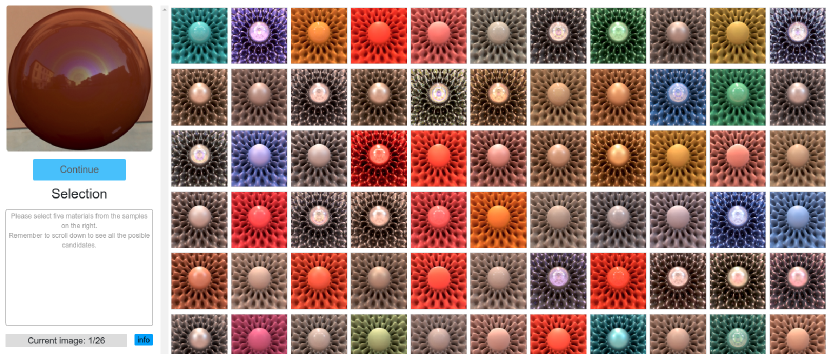
Figure 3. Graphical user interface of the online behavioral experiments. In particular, this screenshot belongs to the Test SH. On the left, the user can see the reference material together with her current selection. On the right, she can observe all the candidate materials. To select one candidate material, the user clicks on the corresponding image and it is automatically added to the selection box on the left.

2.1. Stimuli

We obtain our stimuli from the dataset proposed by Lagunas et al. [2019]. This dataset contains images created using photorealistic computer graphics, with 15 different geometries; six different real-world illuminations ranging from indoor scenarios to urban or natural landscapes; and 100 different materials measured from their real-world counterparts which were pooled from MERL database [Matusik et al., 2003]. We sample the following factors for our experiments:

Geometries

Among the geometries that the dataset contains, we choose the sphere and Havran-2 geometry [Havran et al., 2016]. These are a low and high spatial frequency geometries, respectively, suitable to test how the spatial frequencies of the geometry affect the final appearance of the material and our performance at recognizing it.

• Sphere: Representing a smooth, and low spatial frequency geometry, widely adopted in previous behavioral experiments [Filip et al., 2008; Jarabo et al., 2014; Kerr and Pellacini, 2010; Sun et al., 2017].

• Havran-2: It is a geometry with high spatial frequencies, and with high spatial variations that has been obtained through optimization techniques. Havran-2 surface has had significant success in recent perceptual studies and applications [Lagunas et al., 2019; Guo et al., 2018; Vávra and Filip, 2016; Guarnera et al., 2018].

The stimuli in each different experiment can be observed in Figure 4. The geometry in the reference and candidate samples changes depending on the experiment, the details are as follows:

• Test HH: Both the reference and the candidates depict Havran geometry.

• Test HS: The reference depicts Havran and the candidates depict the sphere.

• Test SH: The reference depicts the sphere while the candidates depict Havran.

• Test SS: Both the reference and the candidates depict the sphere geometry.

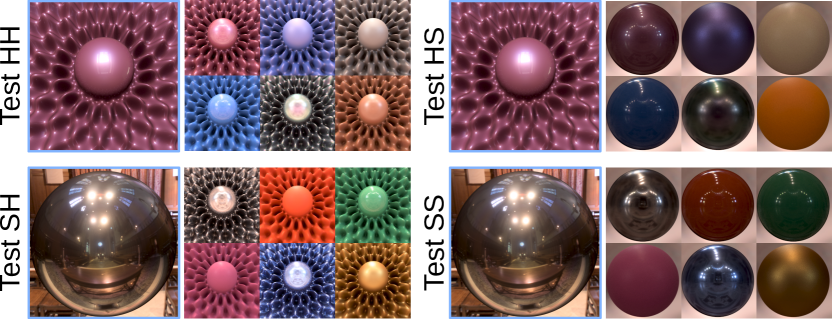
Figure 4. Examples of the stimuli in each different online behavioral experiment. On the left, we show an example of the reference stimuli with one of the six illuminations. On the right, we show a small subset (six out of the 100 materials) of the candidate stimuli with St. Peters illumination.

Illuminations

To prevent a pure matching task, we choose different illuminations between the reference and candidate materials for all behavioral experiments.

• The reference samples depict six different illuminations captured from the real-world. All illuminations can be observed in Figure 5. To have an intuition of the content in the captured illumination, the insets show the RGB intensity for the horizontal purple line. We use all illuminations in the dataset since they contain a mix of spatial frequencies suitable to empirically test how the spatial frequencies of the illumination may affect human performance on material recognition tasks. The illuminations Grace, Ennis, and Uffizi have a broad spatial frequency spectrum, Pisa and Doge mainly contain medium and low spatial frequency content, while Glacier mainly has low spatial frequency content. To simplify the notation, we will refer to them throughout the paper as high-frequency, medium-frequency, and low-frequency illuminations, respectively.

• The candidate samples depict the St. Peters illumination (except in an additional experiment discussed in Section 4 where they depict Doge illumination). St. Peters is an illumination that has been used in the past for several perceptual studies [Fleming et al., 2003; Serrano et al., 2016], and it can be seen in Figure 5. The inset shows the RGB pixel intensity for the horizontal purple line.

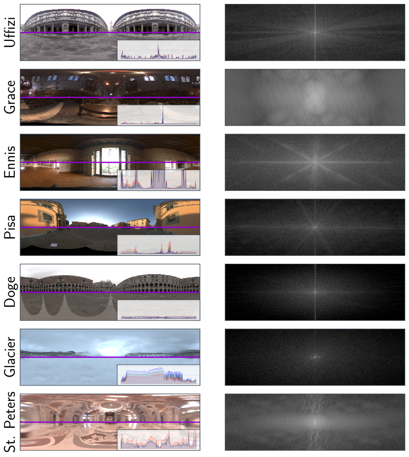
Figure 5. Left: All illuminations depicted in the online behavioral experiments. The inset corresponds to the pixel intensity for the horizontal purple line. Right: Magnitude spectrum of the luminance for each illumination.

To quantify the spatial frequencies of the illuminations, we have employed the high-frequency content measure (HFC) [Brossier et al., 2004]. This measure characterizes the frequencies in a signal by summing linearly-weighted values of the spectral magnitude, thus avoiding to arbitrarily choose a separation between high and low frequencies, or visually assessing the slope of the 1/f amplitude spectrum. A high HFC value means higher frequencies in the signal. Figure 6 shows the HFC for each illumination.

Figure 6. High-frequency content (HFC) measure computed for all the candidate and reference illuminations. We can observe how high-frequency illuminations (Uffizi, Grace, Ennis, St. Peters) also have a high HFC value, medium-frequency illuminations (Pisa, Doge) have a lower HFC value, and, last, low-frequency illuminations (Glacier) have the lowest HFC value.

Materials

We use all the materials from the Lagunas et al. dataset [2019]. The reference trials are sampled uniformly to cover all 100 material samples in the dataset. Examples of the stimuli used in each behavioral experiment are shown in Figure 4, where the image on the left shows the reference material and the right area shows a subset of the candidate materials.

2.2. Participants

The online behavioral experiments were designed to work across platforms on standard web browsers, and they were conducted through the Amazon Mechanical Turk (MTurk) platform. In total, 847 unique users took part in them (368 users belonging to the experiments explained in Section 3, and 479 belonging to the additional experiments explained in Section 4), 44.61% of them female. Among the participants, 62.47% claimed to be familiar with computer graphics, 25.57% had no previous experience and 9.96% declared themselves professionals. We also sampled data regarding the devices used during the experiments: 94.10% used a monitor, 4.30% used a tablet, and 1.60% used a mobile phone. In addition, the most common screen size was 1366x728 px. (42.01% of participants), minimum screen size was 640x360 px. (two people), and a maximum of 2560x1414 px. (one person). Users were not aware of the purpose of the behavioral experiment.

2.3. Procedure

Subjects are shown a reference sample and a group of candidate material samples. Each experiment, HIT in MTurk terminology, consists of 23 unique reference material samples or trials, three of which are sentinels used to detect malicious or lazy users. Users are asked to ”select five material samples which you believe are closer to the one shown in the reference image”. Additionally, we instruct them to make their selection in decreasing order of confidence. We let the users pick five candidate materials because just one answer would provide sparse results. We launched 25 HITs for each experiment and each HIT was answered by six different users. This resulted in a total of 27.000 non-sentinel trials, 12.000 belonging to the four experiments analyzed in Section 3, and 15.000 of them belonging to the five additional experiments discussed in Section 4 (a total of nine different experiments with 25 HITs each, each HIT answered by six users and 20 non-sentinel trials per HIT). Users were not allowed to repeat the same HIT.

The set of materials in the candidate samples does not vary across HITs, however, the position of each sample is randomized for each trial. This has a two-fold purpose: it prevents the user from memorizing the position of the samples, and it prevents them from selecting only the candidate samples that appear at the top of their screen. The reference samples do not repeat materials during a HIT and the reference material is always present among the candidate samples. During the experiment, stimuli keep a constant display size of 300x300 px. for the reference, and of 120x120 px. for the candidate stimuli (except for some of the additional experiments explained in Section 4 where both reference and candidate stimuli are displayed at either 300x300 px. or 120x120 px.). Figure 3 shows a screenshot with the graphical user interface during the behavioral experiments. On the left-hand side, we can observe the selection panel with the current trial and the selection of the current materials. The right-hand side displays the set of candidate materials whereof users can pick their selection. Users were not able to go back and re-do an already answered trial, but they could edit their current selection of five materials until they were satisfied with their choice. Additionally, once the 23 trials of the HIT are answered, to have an intuition about the main features that humans use for material recognition, we asked the user: ”Which visual cues did you consider to perform the test?”.

To minimize worker unreliability, the user performs a brief training before the real test [Welinder et al., 2010]. To avoid giving the user further information about the test, we use a different geometry (Havran-3 [Havran et al., 2016]) during the training phase. In this phase, the items of the interface are explained and the user is given guidance on how to perform the test using just a few images [Garces et al., 2014; Rubinstein et al., 2010; Lagunas et al., 2018].

Sentinels

Each sentinel shows a randomly selected image from the pool of candidates as the reference sample. We consider user answers to the sentinel as valid if they pick the right material within their five selections, regardless of the order. We rejected users that did not correctly answer at least one out of the three sentinel questions. In order to ensure that users answers were well thought and that they were paying attention to the experiment, we also rejected users that took less than five seconds per trial (on average). In the end, we adopt a conservative approach and rejected 19.8% of the participants, gathering 21.660 answers (9.560 belonging to the behavioral experiments explained in Section 3 and 12.100 belonging to the additional experiments explained in Section 4).

3. Results

We investigate which factors have a significant influence on user performance and on the time they took to complete each trial in the four experiments: Test HH, Test HS, Test SH and Test SS. The factors we include are: the reference geometry Gref, the candidate geometry Gcand, and the illumination of the reference sample Iref, as well as their first-order interactions (recall that the illumination of the candidate samples remains constant in these behavioral experiments). We also include the Order of appearance of each trial. We use a general linear mixed model with a binomial distribution for the performance since it is well-suited for binary dependent variables like ours, and a negative binomial distribution for the time, which provides more accurate models than the Poisson distribution by allowing the mean and variance to be different. Since we cannot assume that our observations are independent, we model the potential effect of each particular subject viewing the stimuli as a random effect. Since we have categorical variables among our predictors, we re-code them to dummy variables for the regression. In all our tests, we fix a significance value ($p$-value) of $0.05$. Finally, for factors that present a significant influence, we further perform pairwise comparisons for all their levels (least significant difference pairwise multiple comparison test).

3.1. Analysis of user performance and time

In our online behavioral experiments, we rely on the top-5 accuracy to measure user performance. This metric considers an answer as correct if the reference is among the five candidate materials that the user picked in the trial. Since participants picked five materials ranked in descending order of confidence, the top-1 accuracy could also be considered for our analysis. However, the task they have to solve is not easy and users have an overall top-1 accuracy of 9.21% which yields sparse results. A random selection would yield a top-1 accuracy of 1% and a top-5 accuracy of 5%.

Influence of the geometry

There is a clear effect in user performance when the the geometry changes, regardless if that change happens in the candidate (Gcand, $p=0.005$) or the reference geometry (Gref, $p<0.001$). This is expected, since the geometry plays a key role in how a surface reflects the incoming light and, therefore, will have an impact on the final appearance of the material. Figure 7 shows user performance in terms of top-5 accuracy with a 95% confidence interval when the reference and candidate geometry change jointly (left) or individually (center and right). Users seem to perform better when they have to recognize the material in a high-frequency geometry compared to a low-frequency one. Those results also suggest that changes in the frequencies of the reference geometry may have a bigger impact on user performance than changes in the frequencies of the candidate geometry (i.e., users perform better with a high-frequency reference geometry and low-frequency candidate geometry, compared to a low-frequency reference geometry and a high-frequency candidate geometry).

Figure 7. Left: Top-5 accuracy for each of the four behavioral experiment. Center: Top-5 accuracy for each reference geometry Gref. Right: Top-5 accuracy for the candidate geometry Gcand. We can see how users seem to perform better when the candidate and reference are a high-frequency geometry. All plots have a 95% confidence interval. The names marked with $*$ are found to have statistically significant differences.

Influence of the reference illumination

We observe that the illumination of the reference image has a significant effect on user performance (Iref, $p<0.001$). This is expected since all the materials in a scene are reflecting the light that reaches them, therefore changes in illumination can significantly influence the final appearance of a material, and how we perceive it [Bousseau et al., 2011]. Figure 8, left, shows the top-5 accuracy for each reference illumination and groups of illuminations with statistically indistinguishable performance. We can observe how users seem to have better performance when the surface they are evaluating has been lit with a high-frequency illumination (Ennis, Grace, and Uffizi); while users appear to perform worse in scenes with a low-frequency illumination (Glacier); users show an intermediate performance with a medium-frequency illumination (Doge and Pisa). Moreover, we performed a least significant difference pairwise multiple comparison test to obtain groups of illuminations with statistically indistinguishable performance. These groups can be observed in Figure 8, under the x-axis. If we focus on Iref we can see how high- (green), medium- (blue), and low-frequency (red) illuminations yield groups of similar performance. There is an additional group of statistically indistinguishable performance represented in pink color.

Figure 8. Left: Top-5 accuracy for each reference illumination (Iref). We can see how users seem to perform better with high-frequency illuminations (Uffizi, Grace, Ennis), while their performance is worse with a low-frequency illumination (Glacier). Additionally, they have an intermediate performance for medium-frequency illuminations (Doge and Pisa). Center: Top-5 accuracy for each reference illumination when the candidate geometry (Gcand) changes. We can observe how users appear to perform significantly better with a high-frequency geometry (Havran) and illumination. On the other hand, for low-frequency illuminations, changes in the candidate geometry yield statistically indistinguishable performance. Right: Top-5 accuracy for each reference illumination when the reference geometry (Gref) changes. We can observe how users seem to perform significantly better for all high-frequency illuminations, except for Grace. The horizontal lines under the x-axis represent groups of statistically indistinguishable performance. We can observe how the groups usually cluster high-, medium- and low-frequency illuminations. The reference illuminations marked with $*$ denote significant differences in user performance between geometries for that illumination. The error bars correspond to a 95% confidence interval.

Influence of trial order

The order of appearance of the trials during the experiment does not have a significant influence in users performance (Order, $p=0.391$).

First order interactions

We find that the interaction between the candidate geometry and the reference illumination has a significant effect on user performance ($\text{\emph{Gcand}}*\text{\emph{Iref}}$, $p<0.001$). Users seem to perform better with a high-frequency geometry (compared to a low-frequency one) when the reference stimuli features a high-frequency illumination (Iref=Uffizi, $p=0.019$; Iref=[Grace, Ennis], $p<0.001$). On the other hand, there appears to be no significant changes in performance between a high- and low- frequency candidate geometry when the reference stimuli has a medium- or low-frequency illumination (Iref=Doge, $p=0.453$; Iref=Pisa, $p=0.381$; Iref=Glacier, $p=0.770$). We argue that user performance is driven by the reference sample. When the reference material is lit with a low-frequency illumination, users seem to not be able to properly recognize it. Therefore, changes in the candidate geometry are not relevant to user performance. These results can be seen in Figure 8, center. Furthermore, under the x-axis, we can observe the groups with statistically indistinguishable performance where high-, medium-, and low-frequency illuminations yield groups of similar performance.

We also found out that the interaction between the reference geometry and the reference illumination has a significant impact in user performance ($\text{\emph{Gref}}*\text{\emph{Iref}}$, $p=0.012$). Users seem to show better performance for all illuminations with a high-frequency reference geometry (Gref=Havran, Iref=Uffizi, $p=0.002$; Iref =[Ennis, Pisa, Doge, Glacier], $p<0.001$), except for Grace illumination ($p=0.176$), where the differences in humans performance are statistically indistinguishable. These results, together with the groups of statistically indistinguishable performance, can be seen in Figure 8, right.

In general, we can not conclude that there are significant changes in performance due to the interaction between the candidate and reference geometry (${\text{\emph{Gref}}*\text{\emph{Gcand}}}$, $p=0.407$). Nevertheless, with a low-frequency reference geometry (Gref=sphere), users seem to perform significantly better with a high-frequency candidate geometry (Gcand=Havran, $p=0.009$).

3.1.1. Analysis of the time spent on each trial

To account for time, we measure the number of milliseconds that passed since the trial loaded in their screen and until they picked all five materials and pressed the ”Continue” button.

Influence of trial order

We find that the order of the trials has a significant influence on the average time users spend to answer them ($p<0.001$). Users spend more time in the first questions and that after few trials the average time they spend becomes stable at around 20 seconds per trial (recall that the order does not influence performance). This is expected as users have to familiarize with the experiment during the first iterations. As the test advances, they learn how to interact with it and the time they spend becomes stable. Additional figures and results on the factors that influence the spent time can be found in Appendix A.

3.2. High-level factors driving material recognition

In addition to the analysis, we also try to gain intuition on which high-level factors drive material recognition, investigate how simple image statistics and image histograms correlate with human answers, and analyze highly non-linear statistics in material classification tasks by training a deep neural network.

Visualizing user answers

To gain intuition on which high-level factors humans might use while recognizing materials, we employ a stochastic triplet embedding method called t-STE (t-Student stochastic triplet embedding) [Van Der Maaten and Weinberger, 2012] directly on user answers. This method maps user answers from their original non-numerical domain into a two-dimensional space that can be easily visualized (find additional details in the Appendix B). Figure 9 shows the two-dimensional embeddings after applying the t-STE algorithm to the answers of each online behavioral experiment. Each point in the embedding represents one of the 100 materials from the Lagunas et al. dataset. The insets show the color of each material based on the color classification proposed by Lagunas et al. We can observe how materials are clustered by color and, if we focus in a single color, they seem to be clustered by reflectance properties (for instance, in Test HH, red color cluster, we can observe how on the left there are specular materials while on the right there are diffuse materials). This suggests that users have followed a two-step strategy to recognize the materials, and that the high-level factors driving material recognition might be color first, and the reflectance properties second. At the end of the HIT, users were asked to write the main visual features they used to recognize materials. Out of 368 unique users from the experiments analyzed in Section 3, 273 answered that they have used the colors, and 221 answered that they relied on the reflections. Among them, 157 answered both color and reflections as some of the visual cues they have used to perform the task. This observation, together with the t-STE visualization, strengthens the hypothesis of a two-step strategy.

Figure 9. Visualizations of user answers to each of the four online behavioral experiments (namely Test HH, Test HS, Test SH, and Test SS) using the t-STE algorithm [Van Der Maaten and Weinberger, 2012]. The inset shows the color of each material based on the color classification proposed by Lagunas et al. [2019]. We can see how, for all experiments, materials with similar color properties are grouped together. Furthermore, if we explore the color clusters individually, we can see how there is a second-level arrangement by reflectance properties. These observations suggest that users may be performing a two-step process while recognizing materials where first, they sort them out by color, and second, by reflectance properties.

Image statistics

Previous studies focused on simple image statistics as an attempt to further understand our visual system [Motoyoshi et al., 2007; Adelson, 2008]. Nevertheless, it is argued if our visual system actually derives any aspects of material perception using such simple statistics [Anderson and Kim, 2009; Kim and Anderson, 2010; Olkkonen and Brainard, 2010]. We tested out the correlation between the first four statistical moments of the luminance (considered as the ratio: $L=0.3086*R+0.6094*G+0.0820*B$), the pixel intensity for each color channel independently, and the joint RGB pixel intensity, directly against users top-5 accuracy. To measure correlation we employ a Pearson $\mathcal{P}$ and Spearman $\mathcal{S}$ correlation test. We found out that there is little to no correlation except for the standard deviation of the joint RGB pixel intensity where $\mathcal{P}^{2}=0.43$ ($p<0.001$) and $\mathcal{S}^{2}=0.50$ ($p<0.001$). Additional information can be found in Appendix C.

Image histograms

We also compute the histograms of the RGB pixel intensity, of the luminance, of a Gaussian pyramid [Lee and Lee, 2016], of a Laplacian pyramid [Burt and Adelson, 1983], and of log-Gabor filters designed to simulate the receptive field of the simple cells of the Primary Visual Cortex (V1) [Fischer et al., 2007]. To see how such histograms would perform at classifying materials, we train a support vector machine (SVM) that takes the image histogram as the input and classifies the material in that image. We use a radial basis function kernel (or Gaussian kernel) in the SVM. We use all image histograms that do not feature Havran geometry as the training set and leave the ones with Havran as test set. In the end, the best performing SVM uses the RGB image histogram as the input and achieves a 24.17% top-5 accuracy in the test set.

In addition, we compare the predictions of each SVM directly against human answers. For each reference stimuli we compare the five selections of the user against the five most-likely SVM material predictions for that stimuli. The best SVM uses the histograms of V1-like subband filters and agrees with humans 6.36% of the time. Moreover, we compare histogram similarities against human answers using a chi-square histogram distance [Pele and Werman, 2010]. For a reference image stimuli we measure its similarity against all possible candidate image stimuli and compare the closest five against participants’ answers. The Gaussian pyramid histogram obtained the best result, agreeing with humans 6.29% of the time. These results show how simple statistics, and higher-order image histograms seem not to be capable of fully capturing human behavior. We have added additional results on the SVMs and human agreement in Appendix C.

Image frequencies

To understand if humans performance could be explained by taking into account the spatial frequency of the reference stimuli, at their viewed size, we have added the high-frequency content measure (HFC), and the first four statistical moments of the reference stimuli magnitude spectrum to the factors analyzed in Section 3. We found that the Skewness ($p<0.001$) and Kurtosis ($p<0.001$) of the magnitude spectrum seem to have a significant influence on humans performance; however, they present a very small effect size.

Highly non-linear models

Recent studies suggest that, to understand what surrounds us, our visual system is doing an efficient non-linear encoding of the proximal stimulus (the image input to our visual system) and that highly non-linear models might be able to better capture human perception [Fleming and Storrs, 2019; Delanoy et al., 2020]. Inspired by this hypothesis, we have trained a deep neural network called ResNet [He et al., 2016] employing a loss function suitable to classify the materials in the Lagunas et al. dataset. The images feature the same illuminations as the reference stimuli. We left out the images rendered with Havran geometries for validation and testing purposes, and use the rest during training. To know which material the network classifies we add a softmax layer at the end of the network. The softmax layer outputs the probability of the input image to belong to each material in the dataset. In comparison, the model used by Lagunas et al. does not have the last fully-connected and softmax layer, and it is trained using a triplet loss function aiming for similarity instead of classification. At the end of the training, the model achieves a top-5 accuracy of 89.63% on the test set, suggesting that such models are actually capable of extracting meaningful features from labeled proximal image data (additional details on the training can be found in Appendix D). To gain intuition on how the network has learned, we have used the UMAP (Uniform Manifold Approximation and Projection) algorithm [McInnes and Healy, 2018]. This algorithm aims to reduce the dimensionality of a set of feature vectors while maintaining the global and local structure of their original manifold. Figure 10 shows a two-dimensional visualization of the test set obtained using the 128 features of the fully-connected layer before softmax. We can observe how materials seem to be grouped first by color and then by its reflectance properties suggesting that the model may have used similar high-level factors to humans when classifying materials.

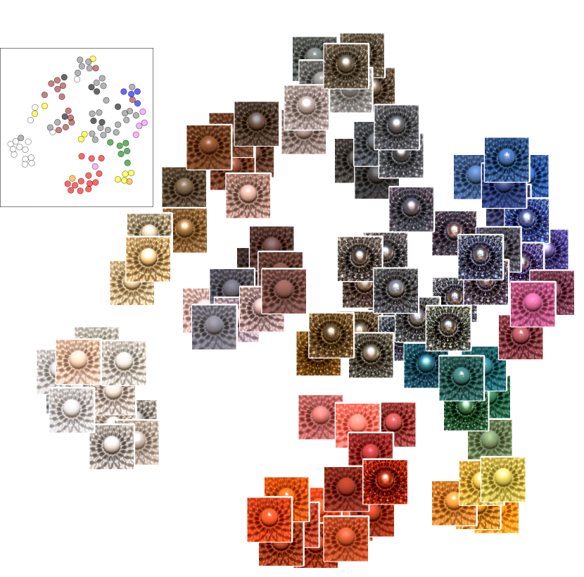
Figure 10. Two-dimensional embedding obtained using the UMAP algorithm [McInnes and Healy, 2018] on the 128 features of the last fully-connected layer of a ResNet model [He et al., 2016] trained to classify materials. The inset shows the color of each material based on the color classification proposed by Lagunas et al. [2019]. We can observe how materials are arranged by color clusters. Moreover, we can observe similarities between this visualization and the t-STE visualization on user answers.

We additionally assess the degree of similarity between the high-level visualization of each online behavioral experiment and the high-level visualization of the deep neural network. We calculate the similarity in a pairwise fashion where we choose a material sample and retrieve its five nearest neighbors in two different low-dimensional representations. Then, we compute the percentage of materials that are the same in both groups of nearest neighbors. We repeat this process for all the materials and calculate the similarity as the average. The low-dimensional representations are obtained with stochastic methods, where the same input can have different results if we vary the parameters. To evaluate the degree of self-similarity, we run the t-STE algorithm [Van Der Maaten and Weinberger, 2012] on each behavioral experiment using five different sets of fully randomly sampled parameters. We obtain a self-similarity value of 0.66, on average across experiments. On the other hand, a set of random low-dimensional representations has a similarity of 0.06, on average. Figure 11 shows the average pairwise similarity normalized by the value of self-similarity and random similarity for all experiments and the deep neural network visualization. If we compare between behavioral experiments, we can observe a decreasing degree of similarity as their stimuli feature fewer frequencies in the spectrum, where Test SS yields the lowest similarity in each of the pairwise comparisons. We argue that Test SS has the lowest similarity because it is the experiment where users have the worst performance, thus yielding a blurry high level visualization. On the other hand, the network is very accurate at classifying materials and yields a high-level visualization with well-defined material clusters. Moreover, if we focus on the deep neural network visualization, we can observe how its similarity values are, in general, on par with those obtained by users in Test HH, Test HS, and Test SH. This result further supports the hypothesis that both humans and deep neural networks may rely on similar high-level visual features for material recognition tasks. However, this is just a preliminary result that may highlight a future avenue of research, and a thorough analysis of the perceptual relationship between deep learning architectures and humans is out of the scope of this paper.

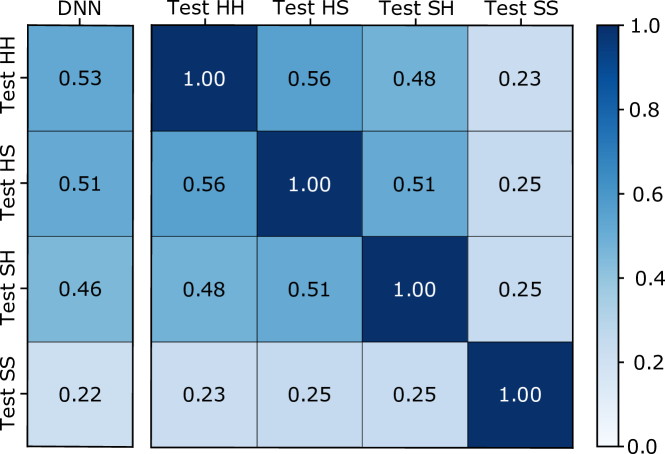
Figure 11. Normalized pairwise similarity for each online behavioral experiment and the deep neural network trained for material classification. We can observe how the pairwise similarity decreases as the stimuli in the experiments cover fewer frequencies in the spectrum, where Test SS has the lowest similarity. Additionally, we can see how the similarities between the neural network and each behavioral experiment are on par with those obtained by humans between Test HH, Test HS, and Test SH.

4. Discussion

From our online behavioral experiments, we have observed that humans appear to perform better at recognizing materials in stimuli with high-frequency illumination and geometry. Moreover, our performance when recognizing materials is poor on low-frequency illuminations, and it remains statistically indistinguishable irrespective of the spatial frequency content in the candidate geometry.

Asymmetric effect of the reference and candidate geometry

It is also interesting to observe that humans seem to have better performance with a high-frequency reference geometry, compared to a high-frequency candidate geometry ($p=0.001$, see Figure 12, left). The number of candidates with respect to the reference could be used as an explanation for this observation, since users may devote more time to inspecting the single reference than the higher number of candidates. At the same time, a lower performance with a high-frequency reference geometry may speak against an inverse optics approach since having multiple candidate materials with the same geometry and illumination could provide a strong cue to inferring the material.

One potential factor that may explain this difference in performance is the different display sizes of the reference (300x300 px.) and the candidate (120x120 px.) stimuli. To test this hypothesis, we have launched two additional experiments where we collect answers on Test HS and Test SH displaying the candidate and the reference stimuli at size 300x300, and other two additional experiments where they are displayed at 120x120 px. We sample the stimuli to cover all the possible combinations of illuminations and materials and keep other technical details as explained in Section 2. We perform an analysis of the gathered data similar to the one explained in Section 3, but using the different experiment type as a factor. From our results we observe that such asymmetric effect remains present when the stimuli are displayed at 300x300 px. ($p<0.001$) and when they are displayed at 120x120 px. ($p<0.001$). Those results can be seen in Figure 12, middle and right. It is also interesting to observe how users have slightly worse performance when the stimuli are displayed at 300x300 px. At such display size only three candidate stimuli per row could be displayed taking into account the most used display size. Thus, seems reasonable to think that the need for additional scrolling could be hampering participants performance.

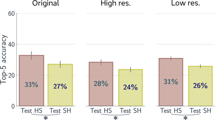
Figure 12. Top-5 accuracy obtained by participants in the original experiment (left), when the stimuli are displayed at 300x300 px. (middle), and at 120x120 px. (right). We can observe how the asymmetric effect of participants performing better when Havran is the reference geometry (TestHS) compared to when it is the candidate (TestSH) remains present when the participants observe the reference and candidate stimuli at identical sizes (middle and right). The $*$ denotes significant differences. The error bars correspond to a 95% confidence interval.

Influence of the candidate illumination

We have seen that humans seem to be better at recognizing materials under high-frequency reference illuminations. However, in Figure 5 and 6 we can see that the St. Peters candidate illumination features a similar frequency content to the reference illuminations where users have better performance. To asses if St. Peters illumination contains a set of frequencies that aids recognizing materials under reference illuminations with a similar set of frequencies, we have launched an additional behavioral experiment. In this experiment we use Doge, a medium-frequency illumination, as the candidate illumination. We sample the stimuli to cover all materials and reference illuminations in Test HH. Other technical details are kept as explained in Section 2. From the data collected (see Figure 13), we can observe how, using Doge as the candidate illumination, humans performance follows a similar distribution to the original experiment (with St. Peters as the candidate illumination). Participants seem to perform better with high-frequency reference illuminations (Uffizi, Grace, Ennis), they perform worse with medium-frequency ones (Pisa), and have their worst performance with low-frequency reference illuminations (Glacier). In addition, participants seem to have slightly better performance with a high-frequency candidate illumination (St. Peters) compared to a medium-frequency one (Doge).

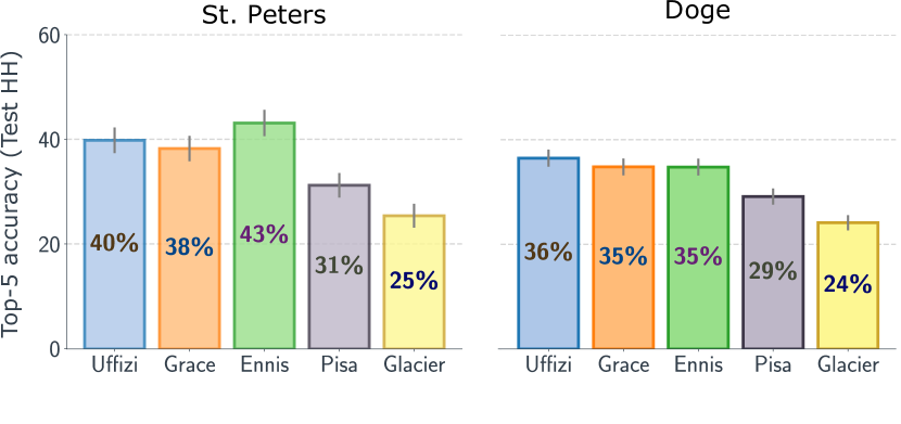
Figure 13. Left: Top-5 accuracy for each reference illumination when St. Peters, a high-frequency illumination, is the candidate illumination. Right: Top-5 accuracy for each reference illumination when Doge, a medium-frequency illumination, is the candidate illumination. Both results have been obtained for Test HH. We can observe how, for both candidate illuminations, participants seem to perform better with high-frequency reference illuminations (Uffizi, Grace, Ennis), they perform worse with medium-frequency ones (Pisa), and have their worst performance with low-frequency reference illuminations (Glacier). In addition, we also observe that participants have slightly better performance when St. Peters (high-frequency illumination) is the candidate illumination. The error bars correspond to a 95% confidence interval.

Interplay between material, geometry, and illumination

We have looked into how geometry, illumination, and their frequencies affect our performance in material recognition tasks. Our stimuli were rendered images in which we varied the frequency of the illumination, and of the underlying geometry of the object present. To better understand how our factors (illumination and geometry) affect the generated stimuli, and thus the proximal stimulus, we offer here a brief description of the rendering equation, providing an explanation of the probable effect of how the frequencies of the geometry and illumination in the 3D scene affect the final, rendered image that is used as a stimulus in our experiments. From the point of view of the rendering equation, the radiance $L_{o}$ at point $x$ in direction $\omega_{o}$, assuming a distant illumination and non-emissive surfaces can be approximated as

(1) $$L_{o}(x,\omega_{o})\approx\int_{\Omega}L_{i}(\omega_{i})\;F(\omega_{i},\omega_{o})\;T(x,\omega_{i},\omega_{o})\;d\omega_{i},$$

where $L_{i}$ accounts for the incoming light, the variable $F$ accounts for the reflectance of the surface, and $T$ depends on the point of the surface we are evaluating, therefore, on the geometry.

The simulation of the radiance $L_{o}$ can be seen as a convolution (spherical rotation) [Ramamoorthi and Hanrahan, 2001] between each signal: incoming radiance $L_{i}$, material $F$ and geometry $T$. Moreover, if we analyze $L_{o}$ in the frequency domain (where $\mathcal{F}$ is the Fourier transform), and apply the convolution theorem ($f*g=\mathcal{F}(f)\cdot\mathcal{F}(g)$) the value of ${\mathcal{F}\big{(}L_{o}\big{)}}$ becomes

(2) $$\mathcal{F}\big{(}L_{o}\big{)}\approx\mathcal{F}\big{(}L_{i}\big{)}\;\mathcal{F}\big{(}F\big{)}\;\mathcal{F}\big{(}T\big{)}.$$

Equation 2 shows how the frequency of the radiance $L_{o}$ in the final image is a multiplication of all the other signals $L_{i}$, $F$, and $T$ in the frequency domain. Thus, the final image will only have the frequencies that are contained within the three other signals. Figure 14 shows how when we convolve two high-frequency signals, the resulting one keeps the high-frequency content; on the other hand, when we convolve a high- and a low-frequency signal, the resulting one has most of its frequencies masked.

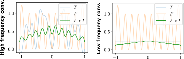
Figure 14. Example of a convolution ($F*T$, green line) between a material ($F$, orange line) and a geometry ($T$, blue line) with different frequency content. Left: We can see how when we convolve a geometry and a material with high spatial frequencies, the resulting convolution also retains high-frequency content. Right: We observe how when geometry has low spatial frequencies and the material has high spatial frequencies, the resulting convolution does not retain high-frequency content. Note that $T$ and $F$ are not necessarily related to a real BRDF or shape from the ones reported in this manuscript.

We can relate the observations made from Equation 2 to the results on user performance that we obtained from the online behavioral experiments. We have seen that users seem to consistently perform better when they recognize materials from high-frequency geometries and illuminations. This finding is supported by Equation 2 since, to avoid filtering the frequencies of the material in the stimuli, it should have a high-frequency geometry and illumination. Moreover, a low-frequency geometry (or illumination) could filter out the frequencies of the illumination (or geometry) and the material, thus yielding fewer visual features on the final image and, as a result, worse users performance. This is consistent with our findings from the analysis of first-order interactions for users performance in Section 3.1.

Material categories

We have seen that the reflectance properties seem to be one of the main high-level factors driving material recognition. In this regard, we have also investigated users performance using the classification by reflectance type proposed by Lagunas et al. [2019], where the MERL database is divided into eight different categories with similar reflectance properties. On average, users perform best on acrylics, with a top-5 accuracy of 45.45%, while they have their worst performance with organics, with an accuracy of 10.22%. Figure 15 shows the top-5 accuracy for each category in each reference illumination. Firstly, we observe that users seem to perform better with high-frequency illuminations (Uffizi, Grace, Ennis). However, we can see how fabrics and organics do not follow this trend. We argue that fabrics and organics contain mostly materials with a diffuse surface reflectance (low-frequency) that clamp the frequencies of the illumination and, therefore, yield fewer cues in the final stimulus that is input to our visual system.

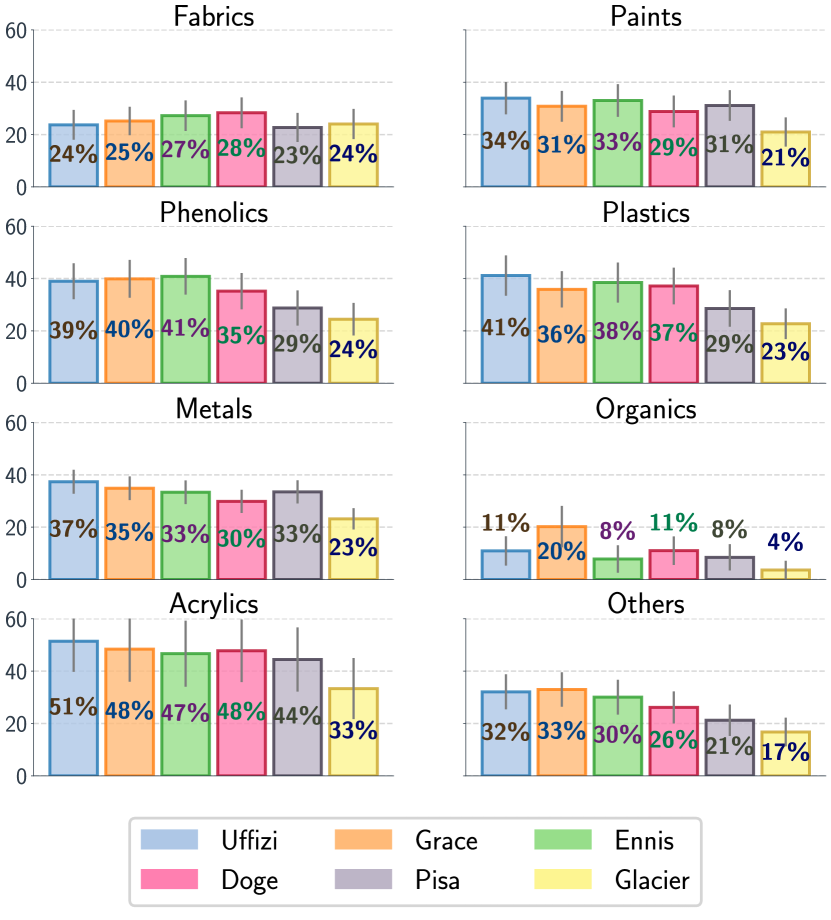
Figure 15. Users performance, in terms of top-5 accuracy, for material recognition tasks taking into account the reflectance of the materials. We can observe how, on average, users perform better for high-frequency illuminations (Uffizi, Grace, and Ennis). Also, we can see how for classes, like fabrics or organics, containing materials with diffuse surface reflectance (low-frequency), users do not have better performance with broad frequency content illuminations. We argue that, since they have a low-frequency surface reflectance, even though there is a high-frequency illumination, those frequencies cannot be represented on the final stimulus that is input to our visual system.

5. Conclusions

In this work, we have presented a thorough and systematic analysis of the interplay between geometry, illumination, and their spatial frequencies in human performance recognizing materials. We launched rigorous crowd-sourced online behavioral experiments where participants had to solve a material recognition task between a reference and a set of candidate samples. From our experiments, we have observed that, in general, humans appear to be better at recognizing materials in a high-frequency illumination and geometry. We found that simple image statistics, image histograms, and histograms of V1-like subband filters are not capable of capturing human behavior, and, additionally, explored highly non-linear statistics by training a deep neural network on material classification tasks. We showed that deep neural networks can accurately perform material classification, which suggests that they are capable of encoding and extracting meaningful information from labeled proximal image data. In addition, we gained intuition on which are the main high-level factors that humans and those highly non-linear statistics use for material recognition and found preliminary evidence that such statistics and humans may share similar high-level factors for material recognition tasks.

Limitations and future work

To collect data for the online behavioral experiment we have relied on the Lagunas et al. [Lagunas et al., 2019] dataset which contains images of a diverse set of materials, geometries, and illuminations that faithfully resemble their real-world counterparts. This database focuses on isotropic materials, which are capable of modeling only a subset of real-world materials. A systematic and comprehensive analysis of other heterogeneous materials, or an extension of this study to other non-photorealistic domains, remains to be done. Our stimuli were rendered using the sphere and Havran geometry, although those surfaces have been widely used in the literature [Lagunas et al., 2019; Serrano et al., 2016; Jarabo et al., 2014; Havran et al., 2016], introducing new geometries could help to further analyze the contribution of the spatial frequencies of the geometry in our perception of material appearance [Nishida and Shinya, 1998]. Moreover, to select our stimuli, we characterized the frequency content of real-world illuminations using the high-frequency content measure [Brossier et al., 2004]. We focus on real-world illuminations, which are by definition broadband, therefore, we do not impose nor limit their frequency distribution in our analyses; carefully controlling the spatial frequency of the stimuli via filtering in order to isolate frequency bands and study their individual contribution to the process of material recognition is an interesting avenue of research.

In our additional experiments, we have investigated the asymmetric effect in performance with a high-frequency reference geometry, compared to a high-frequency candidate geometry when all stimuli are displayed at the same size. A rigorous study of the interplay between display size, the spatial frequencies of the stimuli, and how this affects humans performance on material recognition remains an interesting line of future work. Furthermore, despite the fact that our neural network was trained to classify materials, without any sort of perceptual information, it achieved an agreement with participants answers of 22.43%. This does not prove that the neural network follows the same mechanisms as humans do when performing these tasks. However, this result together with the increase in popularity of deep neural networks, makes the analysis of the perceptual relationship between learned features and the features that our visual system uses to recognize materials a promising avenue to explore. Last, we hope that our analyses will provide relevant insights that will help shed light on the underlying perceptual processes that occur when we recognize materials and, in particular, on how the confounding factors of geometry and illumination affect our perception of material appearance.

Appendix

Appendix A Additional results on the influence of time

Additional details on the time that each participant spent doing the online behavioral experiment. In Figure 16 we can see how the time spent to answer each trial becomes stable as the behavioral experiment advances.

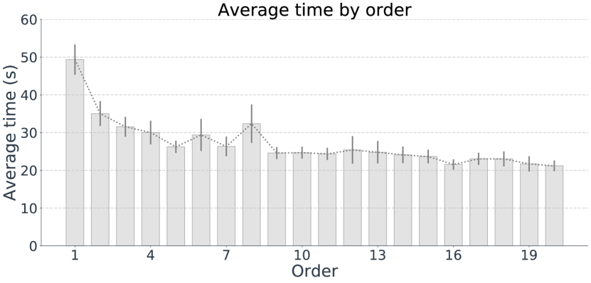
Figure 16. Average time the users spent for each trial according to the order of appearance during the online behavioral experiment. We can observe how, as the user progresses through the experiment, the time spent on each trial becomes stable. The error bars correspond to a 95% confidence interval.

Influence of reference illumination

The reference illumination Iref influences the time users spend to answer each trial ($p=0.001$). Users spend more time when the stimuli are lit with Ennis illumination while they are the fastest when the illumination is Doge.

We did not find a significant influence of the reference geometry Gref or candidate geometry Gcand in the average time each user spent to answer each trial.

First order interactions

We observe that users take significantly longer to answer the trials when both the reference geometry and the candidate geometry change (Gref $*$ Gcand, $p=0.001$). This happens in the case where the reference geometry has mostly low spatial frequency content and the candidate geometry changes (Gcand=sphere, $p$=0.002); and when the reference has mostly low spatial frequency (Gref=sphere, $p$=0.001) and the candidate geometry changes.

Appendix B Additional details on the t-STE algorithm

The t-STE algorithm aims to obtain an n-dimensional embedding that satisfies as many qualitative comparisons of the type ”A is more similar to B than C” as possible. In our case, a two-dimensional embedding which is easier to visualize. Nevertheless, in the user studies, we have asked participants to select five materials from a pool of candidates and we do not have such qualitative comparisons. However, we can assume that the selection of the users will be closer (more similar) to the reference than any other material that was not selected. Based on this assumption, we generate triplets where the user selection is more similar to the reference material than any other random material that is not within the 5 selected materials. We repeat this process ten times for each of the 5 materials selected by the user making sure that the new randomly sampled material has not been randomly selected already nor that it belongs to the pool of 5 selected materials. To run the t-STE we set a learning rate of 1, and an $\alpha=25$ (degrees of freedom of the Student-t kernel). Additionally, we apply a logarithmic transformation to the loss value of the t-STE. Those parameters are the same for the answers of the four experiments.

Appendix C Additional details on image statistics

To measure the correlation between image statistics and users performance we employ a Pearson $\mathcal{P}$ and Spearman $\mathcal{S}$ correlation test with a significance value ($p$-value) of 0.05. The value $\mathcal{P}^{n}$ represents the Pearson correlation for the $n^{\text{th}}$ statistical moment (same applies for the Spearman $\mathcal{S}^{n}$ correlation).

Luminance

We analyze if the moments of the luminance of each material image have a direct influence on users performance. We found that the moments of the luminance are not correlated with users performance: $\mathcal{P}^{1}=-0.14$ ($p=0.17$), $\mathcal{S}^{1}=-0.15$ ($p=0.15$), $\mathcal{P}^{2}=0.02$ ($p=0.83$), $\mathcal{S}^{2}=-0.03$ ($p=0.78$), $\mathcal{P}^{3}=0.03$ ($p=0.77$), $\mathcal{S}^{3}=0.03$ ($p=0.78$), $\mathcal{P}^{4}=0.01$ ($p=0.94$), $\mathcal{S}^{4}=0.05$ ($p=0.65$).

RGB image

We analyze if the moments of the joint RGB intensity of each material image have a direct influence on users performance. We found that the moments of the joint RGB intensity have little to no correlation with users performance except for the standard deviation: $\mathcal{P}^{1}=-0.02$ ($p=0.79$), $\mathcal{S}^{1}=-0.06$ ($p=0.51$), $\mathcal{P}^{2}=0.43$ ($p<0.001$), $\mathcal{S}^{2}=0.50$ ($p<0.001$), $\mathcal{P}^{3}=0.16$ ($p=0.09$), $\mathcal{S}^{3}=0.22$ ($p=0.02$), $\mathcal{P}^{4}=-0.1$ ($p=0.30$), $\mathcal{S}^{4}=-0.06$ ($p=0.52$).

We also tested out the correlation for each channel and found out that for all the channels there is no correlation for any of the first 4 statistical moments.

Red channel

On the red channel there seems to be a slight positive linear correlation between the fourth moment (kurtosis) and users performance. All the other statistics show no significant correlation: $\mathcal{P}^{1}=-0.10$ ($p=0.29$), $\mathcal{S}^{1}=-0.08$ ($p=0.42$), $\mathcal{P}^{2}=0.03$ ($p=0.60$), $\mathcal{S}^{2}=-0.02$ ($p=0.87$), $\mathcal{P}^{3}=0.07$ ($p=0.46$), $\mathcal{S}^{3}=0.07$ ($p=0.51$), $\mathcal{P}^{4}=0.20$ ($p=0.04$), $\mathcal{S}^{4}=0.15$ ($p=0.13$).

Green channel

There is no correlation between any statistics on the green channel: $\mathcal{P}^{1}=-0.04$ ($p=0.66$), $\mathcal{S}^{1}=-0.0.$ ($p=0.74$), $\mathcal{P}^{2}=0.03$ ($p=0.55$), $\mathcal{S}^{2}=0.04$ ($p=0.67$), $\mathcal{P}^{3}=0.05$ ($p=0.64$), $\mathcal{S}^{3}=0.06$ ($p=0.53$), $\mathcal{P}^{4}=0.05$ ($p=0.63$), $\mathcal{S}^{4}=0.01$ ($p=0.94$).

Blue channel

Similar to the green channel, the blue does not show any correlation for the first 4 statistical moments: $\mathcal{P}^{1}=0.03$ ($p=0.72$), $\mathcal{S}^{1}=-0.004$ ($p=0.93$), $\mathcal{P}^{2}=0.06$ ($p=0.52$), $\mathcal{S}^{2}=0.01$ ($p=0.95$), $\mathcal{P}^{3}=0.13$ ($p=0.19$), $\mathcal{S}^{3}=0.10$ ($p=0.30$), $\mathcal{P}^{4}=0.16$ ($p=0.11$), $\mathcal{S}^{4}=-0.05$ ($p=0.61$).

C.1. Additional results on the SVMs and histogram similarity

We have trained a total of 6 support vector machine models, each of them using a different input: RGB pixel intensity, luminance intensity, Gaussian pyramid pixel intensity [Lee and Lee, 2016], Laplacian pyramid pixel intensity [Burt and Adelson, 1983], joining the Gaussian and Laplacian pyramids, and using log-Gabor filters [Fischer et al., 2007]. For each of them the SVM achieved a top-5 accuracy in the test set of: 24.17%, 15.16%, 22.50%, 6.33%, 7.52%, and 16.33%, respectively. In addition, we have compared how the SVM predictions agreed with humans’ answers from the online behavioral experiments. For each SVM the agreement is: 4.24%, 4.33%, 4.34%, 5.04%, 4.97%, and 6.36% respectively. Last, we have also computed the histogram similarity using a chi-squared distance. Then, we have taken the five closest samples and compared that with human answers. We do that for each of the five different histograms and each achieves an agreement of: 5.95%, 5.45%, 6.29%, 4.97%, 5.04%, and 5.07% respectively.

Appendix D Additional details on ResNet training

To train the 35 layers ResNet (34 of the original model plus an additional fully connected)  [He et al., 2016] we have employed the dataset introduced by Lagunas et al. [Lagunas et al., 2019], which contains renderings of materials with different illuminations and geometries. We keep the images rendered with Havran-3 geometry for validation purposes and Havran geometry for testing. All the other images are used for training. To train the model to classify materials we use a soft cross-entropy loss where samples that do not belong to the same class are penalized [Szegedy et al., 2015]. The loss function takes the probabilities output of the softmax layer and penalizes when they give a high probability to the materials that do not belong to the input image. The images input to the model are resized to 224x224 px. The parameters of the model are initialized using a pretrained version on ImageNet dataset [Deng et al., 2009]. We use the ADAM algorithm [Kingma and Ba, 2014] as the optimizer. The model has been trained during 50 iterations starting at a learning rate of $10^{-3}$ and decayed by a factor of 10 at the iteration 20, 35, and 45; the batch-size was set to 64 images. We use the PyTorch framework and use an Nvidia 2080Ti GPU.

References

- [1]
- Adelson [2000] EH Adelson. 2000. Lightness perception and lightness illusions. The new cognitive neurosciences.
- Adelson [2001] Edward H Adelson. 2001. On seeing stuff: the perception of materials by humans and machines. In Human Vision and Electronic Imaging VI, Vol. 4299. International Society for Optics and Photonics, 1–13.
- Adelson [2008] Edward H Adelson. 2008. Image statistics and surface perception. In Human Vision and Electronic Imaging XIII, Vol. 6806. International Society for Optics and Photonics, 680602.
- Anderson [2011] Barton L Anderson. 2011. Visual perception of materials and surfaces. Current Biology 21, 24 (2011), R978–R983.
- Anderson and Kim [2009] Barton L Anderson and Juno Kim. 2009. Image statistics do not explain the perception of gloss and lightness. Journal of Vision (JOV) 9, 11 (2009), 10–10.
- Beck and Prazdny [1981] Jacob Beck and Slava Prazdny. 1981. Highlights and the perception of glossiness. Attention, Perception, & Psychophysics 30, 4 (1981), 407–410.
- Bell et al. [2015] Sean Bell, Paul Upchurch, Noah Snavely, and Kavita Bala. 2015. Material recognition in the wild with the materials in context database. In Proceedings of the IEEE Conference on Computer Vision and Pattern Recognition (CVPR). 3479–3487.
- Bloj et al. [1999] Marina G Bloj, Daniel Kersten, and Anya C Hurlbert. 1999. Perception of three-dimensional shape influences colour perception through mutual illumination. Nature 402, 6764 (1999), 877.
- Bousseau et al. [2011] Adrien Bousseau, Emmanuelle Chapoulie, Ravi Ramamoorthi, and Maneesh Agrawala. 2011. Optimizing environment maps for material depiction. In Computer Graphics Forum, Vol. 30. Wiley Online Library, 1171–1180.
- Brady and Oliva [2012] Timothy Brady and Aude Oliva. 2012. Spatial frequency integration during active perception: perceptual hysteresis when an object recedes. Frontiers in Psychology 3 (2012), 462.
- Brossier et al. [2004] Paul Brossier, Juan Pablo Bello, and Mark D Plumbley. 2004. Real-time temporal segmentation of note objects in music signals. In Proceedings of ICMC 2004, the 30th Annual International Computer Music Conference.
- Burt and Adelson [1983] Peter Burt and Edward Adelson. 1983. The Laplacian pyramid as a compact image code. IEEE Transactions on communications 31, 4 (1983), 532–540.
- Delanoy et al. [2020] Johanna Delanoy, Manuel Lagunas, Ignacio Galve, Diego Gutierrez, Ana Serrano, Roland Fleming, and Belen Masia. 2020. The Role of Objective and Subjective Measures in Material Similarity Learning. In ACM SIGGRAPH 2020 Posters. Article 51, 2 pages.
- Deng et al. [2009] Jia Deng, Wei Dong, Richard Socher, Li-Jia Li, Kai Li, and Li Fei-Fei. 2009. Imagenet: A large-scale hierarchical image database. In Proceedings of the IEEE Conference on Computer Vision and Pattern Recognition (CVPR). Ieee, 248–255.
- Dror et al. [2001a] Ron O Dror, Edward H Adelson, and Alan S Willsky. 2001a. Estimating surface reflectance properties from images under unknown illumination. In Human Vision and Electronic Imaging VI, Vol. 4299. International Society for Optics and Photonics, 231–243.
- Dror et al. [2001b] Ron O Dror, Edward H Adelson, and Alan S Willsky. 2001b. Surface reflectance estimation and natural illumination statistics.
- Faul [2019] Franz Faul. 2019. The influence of Fresnel effects on gloss perception. Journal of Vision (JOV) 19, 13 (2019), 1–1.
- Filip et al. [2008] Jirí Filip, Mike J Chantler, Patrick R Green, and Michal Haindl. 2008. A psychophysically validated metric for bidirectional texture data reduction. ACM Transactions on Graphics (TOG) 27, 5 (2008), 138–1.
- Fischer et al. [2007] Sylvain Fischer, Filip Šroubek, Laurent Perrinet, Rafael Redondo, and Gabriel Cristóbal. 2007. Self-invertible 2D log-Gabor wavelets. International Journal of Computer Vision 75, 2 (2007), 231–246.
- Fleming [2014] Roland W. Fleming. 2014. Visual perception of materials and their properties. Vision Research 94 (2014), 62 – 75.
- Fleming and Bülthoff [2005] Roland W Fleming and Heinrich H Bülthoff. 2005. Low-level image cues in the perception of translucent materials. ACM Transactions on Applied Perception (TAP) 2, 3 (2005), 346–382.
- Fleming et al. [2001] Roland W Fleming, Ron O Dror, and Edward H Adelson. 2001. How do humans determine reflectance properties under unknown illumination? (2001).
- Fleming et al. [2003] Roland W Fleming, Ron O Dror, and Edward H Adelson. 2003. Real-world illumination and the perception of surface reflectance properties. Journal of Vision (JOV) 3, 5 (2003), 3–3.
- Fleming et al. [2015a] Roland W Fleming, Karl R Gegenfurtner, and Shin’ya Nishida. 2015a. Visual perception of materials: the science of stuff. Vision Research 109 (2015), 123–124.
- Fleming et al. [2015b] Roland W. Fleming, Shin’ya Nishida, and Karl R. Gegenfurtner. 2015b. Perception of material properties. Vision Research 115 (2015), 157 – 162.
- Fleming and Storrs [2019] Roland W Fleming and Katherine R Storrs. 2019. Learning to see stuff. Current Opinion in Behavioral Sciences 30 (2019), 100–108.
- Fleming et al. [2013] Roland W Fleming, Christiane Wiebel, and Karl Gegenfurtner. 2013. Perceptual qualities and material classes. Journal of Vision (JOV) 13, 8 (2013), 9–9.
- Garces et al. [2014] Elena Garces, Aseem Agarwala, Diego Gutierrez, and Aaron Hertzmann. 2014. A Similarity Measure for Illustration Style. ACM Transactions on Graphics (Proc. SIGGRAPH 2014) 33, 4 (2014).
- Ged et al. [2010] Guillaume Ged, Gaël Obein, Zaccaria Silvestri, Jean Le Rohellec, and Françoise Viénot. 2010. Recognizing real materials from their glossy appearance. Journal of Vision (JOV) 10, 9 (2010), 18–18.
- Geisler [2008] Wilson S Geisler. 2008. Visual perception and the statistical properties of natural scenes. Annual Review of Psychology 59 (2008), 167–192.
- Giesel and Zaidi [2013] Martin Giesel and Qasim Zaidi. 2013. Frequency-based heuristics for material perception. Journal of Vision (JOV) 13, 14 (2013), 7–7.
- Guarnera et al. [2018] Dar’ya Guarnera, Giuseppe Claudio Guarnera, Matteo Toscani, Mashhuda Glencross, Baihua Li, Jon Yngve Hardeberg, and Karl R. Gegenfurtner. 2018. Perceptually Validated Analytical BRDFs Parameters Remapping. In ACM SIGGRAPH 2018 Talks. Article Article 17, 2 pages.
- Guo et al. [2018] Jie Guo, Yanwen Guo, Jingui Pan, and Wenzhou Lu. 2018. Brdf analysis with directional statistics and its applications. IEEE Transactions on Visualization and Computer Graphics (TVCG) (2018).
- Havran et al. [2016] Vlastimil Havran, Jiri Filip, and Karol Myszkowski. 2016. Perceptually Motivated BRDF Comparison using Single Image. Computer Graphics Forum (2016).
- Hawken and Parker [1987] Michael J Hawken and Andrew J Parker. 1987. Spatial properties of neurons in the monkey striate cortex. Proceedings of the Royal society of London. Series B. Biological sciences 231, 1263 (1987), 251–288.
- He et al. [2016] Kaiming He, Xiangyu Zhang, Shaoqing Ren, and Jian Sun. 2016. Deep residual learning for image recognition. In Proceedings of the IEEE Conference on Computer Vision and Pattern Recognition (CVPR). 770–778.
- Hunter et al. [1937] Richard S Hunter et al. 1937. Methods of determining gloss. NBS Research paper RP 958 (1937).
- Jarabo et al. [2014] Adrian Jarabo, Hongzhi Wu, Julie Dorsey, Holly Rushmeier, and Diego Gutierrez. 2014. Effects of Approximate Filtering on the Appearance of Bidirectional Texture Functions. IEEE Trans. on Visualization and Computer Graphics 20, 6 (2014).
- Julesz [1962] Bela Julesz. 1962. Visual pattern discrimination. IRE transactions on Information Theory 8, 2 (1962), 84–92.
- Kawato et al. [1993] Mitsuo Kawato, Hideki Hayakawa, and Toshio Inui. 1993. A forward-inverse optics model of reciprocal connections between visual cortical areas. Network: Computation in Neural Systems 4, 4 (1993), 415–422.
- Kerr and Pellacini [2010] William B Kerr and Fabio Pellacini. 2010. Toward evaluating material design interface paradigms for novice users. In ACM Transactions on Graphics (TOG), Vol. 29. ACM, 35.
- Kersten et al. [2004] Daniel Kersten, Pascal Mamassian, and Alan Yuille. 2004. Object perception as Bayesian inference. Annual Review of Psychology 55 (2004), 271–304.
- Kim and Anderson [2010] Juno Kim and Barton L Anderson. 2010. Image statistics and the perception of surface gloss and lightness. Journal of Vision (JOV) 10, 9 (2010), 3–3.
- Kingma and Ba [2014] Diederik P Kingma and Jimmy Ba. 2014. Adam: A method for stochastic optimization. arXiv preprint arXiv:1412.6980 (2014).
- Lagunas et al. [2018] Manuel Lagunas, Elena Garces, and Diego Gutierrez. 2018. Learning icons appearance similarity. Multimedia Tools and Applications (2018), 1–19.
- Lagunas et al. [2019] Manuel Lagunas, Sandra Malpica, Ana Serrano, Elena Garces, Diego Gutierrez, and Belen Masia. 2019. A Similarity Measure for Material Appearance. ACM Transactions on Graphics (Proc. SIGGRAPH 2019) 38, 4 (2019).
- Lee and Lee [2016] Seohyung Lee and Daeho Lee. 2016. Fusion of IR and Visual Images Based on Gaussian and Laplacian Decomposition Using Histogram Distributions and Edge Selection. Mathematical Problems in Engineering 2016 (2016).
- Leloup et al. [2010] Frédéric B Leloup, Michael R Pointer, Philip Dutré, and Peter Hanselaer. 2010. Geometry of illumination, luminance contrast, and gloss perception. JOSA A 27, 9 (2010), 2046–2054.
- Li and Fritz [2012] Wenbin Li and Mario Fritz. 2012. Recognizing materials from virtual examples. In European Conference on Computer Vision (ECCV). Springer, 345–358.
- Maloney and Brainard [2010] Laurence T Maloney and David H Brainard. 2010. Color and material perception: Achievements and challenges. Journal of Vision (JOV) 10, 9 (2010), 19–19.
- Mao et al. [2019] Ruiquan Mao, Manuel Lagunas, Belen Masia, and Diego Gutierrez. 2019. The Effect of Motion on the Perception of Material Appearance. In Proceedings of the ACM Symposium on Applied Perception (SAP). ACM, Article 16, 9 pages.
- Marlow et al. [2012] Phillip J Marlow, Juno Kim, and Barton L Anderson. 2012. The perception and misperception of specular surface reflectance. Current Biology 22, 20 (2012), 1909–1913.
- Matusik et al. [2003] Wojciech Matusik, Hanspeter Pfister, Matt Brand, and Leonard McMillan. 2003. A Data-Driven Reflectance Model. ACM Transactions on Graphics (TOG) 22, 3 (July 2003), 759–769.
- McInnes and Healy [2018] Leland McInnes and John Healy. 2018. Umap: Uniform manifold approximation and projection for dimension reduction. arXiv preprint arXiv:1802.03426 (2018).
- Motoyoshi et al. [2007] Isamu Motoyoshi, Shin’ya Nishida, Lavanya Sharan, and Edward H Adelson. 2007. Image statistics and the perception of surface qualities. Nature 447, 7141 (2007), 206–209.
- Nagai et al. [2015] Takehiro Nagai, Toshiki Matsushima, Kowa Koida, Yusuke Tani, Michiteru Kitazaki, and Shigeki Nakauchi. 2015. Temporal properties of material categorization and material rating: visual vs non-visual material features. Vision Research 115 (2015), 259 – 270. Perception of Material Properties (Part II).
- Nishida and Shinya [1998] Shin’ya Nishida and Mikio Shinya. 1998. Use of image-based information in judgments of surface-reflectance properties. JOSA A 15, 12 (1998), 2951–2965.
- Obein et al. [2004] Gaë Obein, Kenneth Knoblauch, and Françise Viéot. 2004. Difference scaling of gloss: Nonlinearity, binocularity, and constancy. Journal of Vision (JOV) 4, 9 (2004), 4–4.
- Oliva and Torralba [2001] Aude Oliva and Antonio Torralba. 2001. Modeling the shape of the scene: A holistic representation of the spatial envelope. International Journal of Computer Vision (IJCV) 42, 3 (2001), 145–175.
- Olkkonen and Brainard [2010] Maria Olkkonen and David H Brainard. 2010. Perceived glossiness and lightness under real-world illumination. Journal of Vision (JOV) 10, 9 (2010), 5–5.
- Olkkonen and Brainard [2011] Maria Olkkonen and David H Brainard. 2011. Joint effects of illumination geometry and object shape in the perception of surface reflectance. i-Perception 2, 9 (2011), 1014–1034.
- Palmer [1975] Stephen E Palmer. 1975. Visual perception and world knowledge: Notes on a model of sensory-cognitive interaction. Explorations in Cognition (1975), 279–307.
- Pele and Werman [2010] Ofir Pele and Michael Werman. 2010. The quadratic-chi histogram distance family. In European conference on computer vision. Springer, 749–762.
- Pizlo [2001] Zygmunt Pizlo. 2001. Perception viewed as an inverse problem. Vision Research 41, 24 (2001), 3145–3161.
- Ramamoorthi and Hanrahan [2001] Ravi Ramamoorthi and Pat Hanrahan. 2001. An efficient representation for irradiance environment maps. In Proceedings of the Annual conference on Computer Graphics and Interactive Techniques. 497–500.
- Rubinstein et al. [2010] Michael Rubinstein, Diego Gutierrez, Olga Sorkine, and Ariel Shamir. 2010. A Comparative Study of Image Retargeting. ACM Transactions on Graphics (Proc. SIGGRAPH Asia 2010) 29, 6 (2010), 160:1–160:10.
- Schaffalitzky and Zisserman [2001] Frederik Schaffalitzky and Andrew Zisserman. 2001. Viewpoint invariant texture matching and wide baseline stereo. In Proceedings of the IEEE International Conference on Computer Vision (ICCV), Vol. 2. IEEE, 636–643.
- Schiller et al. [1976] Peter H Schiller, Barbara L Finlay, and Susan F Volman. 1976. Quantitative studies of single-cell properties in monkey striate cortex. I. Spatiotemporal organization of receptive fields. Journal of neurophysiology 39, 6 (1976), 1288–1319.
- Schlüter and Faul [2019] Nick Schlüter and Franz Faul. 2019. Visual shape perception in the case of transparent objects. Journal of Vision (JOV) 19, 4 (2019), 24–24.
- Serrano et al. [2016] Ana Serrano, Diego Gutierrez, Karol Myszkowski, Hans-Peter Seidel, and Belen Masia. 2016. An Intuitive Control Space for Material Appearance. ACM Transactions on Graphics (TOG) 35, 6, Article 186 (Nov. 2016), 186:1–186:12 pages.
- Sève [1993] Robert Sève. 1993. Problems connected with the concept of gloss. Color Research & Application 18, 4 (1993), 241–252.
- Sharan et al. [2009] Lavanya Sharan, Ruth Rosenholtz, and Edward Adelson. 2009. Material perception: What can you see in a brief glance? Journal of Vision (JOV) 9, 8 (2009), 784–784.
- Sharan et al. [2008] Lavanya Sharan, Ruth Rosenholtz, and Edward H Adelson. 2008. Eye movements for shape and material perception. Journal of Vision (JOV) 8, 6 (2008), 219–219.
- Sun et al. [2017] Tiancheng Sun, Ana Serrano, Diego Gutierrez, and Belen Masia. 2017. Attribute-preserving gamut mapping of measured BRDFs. In Computer Graphics Forum, Vol. 36. Wiley Online Library, 47–54.
- Szegedy et al. [2015] Christian Szegedy, Vincent Vanhoucke, Sergey Ioffe, Jonathon Shlens, and Zbigniew Wojna. 2015. Rethinking the inception architecture for computer vision. arXiv. (2015).
- Thompson et al. [2011] William Thompson, Roland Fleming, Sarah Creem-Regehr, and Jeanine Kelly Stefanucci. 2011. Visual Perception from a Computer Graphics Perspective (1st ed.). A. K. Peters, Ltd., Natick, MA, USA.
- Thompson et al. [2016] William Thompson, Roland Fleming, Sarah Creem-Regehr, and Jeanine Kelly Stefanucci. 2016. Visual perception from a computer graphics perspective. AK Peters/CRC Press.
- Van Der Maaten and Weinberger [2012] Laurens Van Der Maaten and Kilian Weinberger. 2012. Stochastic triplet embedding. In Machine Learning for Signal Processing (MLSP), 2012 IEEE International Workshop on. IEEE, 1–6.
- Vangorp et al. [2007] Peter Vangorp, Jurgen Laurijssen, and Philip Dutré. 2007. The Influence of Shape on the Perception of Material Reflectance. ACM Transactions on Graphics (TOG) 26, 3, Article 77 (July 2007).
- Vávra and Filip [2016] Radomír Vávra and Jirí Filip. 2016. Minimal sampling for effective acquisition of anisotropic BRDFs. In Computer Graphics Forum, Vol. 35. Wiley Online Library, 299–309.
- Wang et al. [2016] Ting-Chun Wang, Jun-Yan Zhu, Ebi Hiroaki, Manmohan Chandraker, Alexei A Efros, and Ravi Ramamoorthi. 2016. A 4D light-field dataset and CNN architectures for material recognition. In European Conference on Computer Vision. Springer, 121–138.
- Welinder et al. [2010] Peter Welinder, Steve Branson, Pietro Perona, and Serge J Belongie. 2010. The multidimensional wisdom of crowds. In Advances in Neural Information Processing Systems (NeurIPS). 2424–2432.
- Zhang et al. [2015] Fan Zhang, Huib de Ridder, and Sylvia Pont. 2015. The influence of lighting on visual perception of material qualities. In Human Vision and Electronic Imaging XX, Vol. 9394. International Society for Optics and Photonics, 93940Q.