Green’s function for the fractional KdV equation on the periodic domain via Mittag–Leffler’s function

Abstract.

The linear operator $c+(-\Delta)^{\alpha/2}$, where $c>0$ and $(-\Delta)^{\alpha/2}$ is the fractional Laplacian on the periodic domain, arises in the existence of periodic travelling waves in the fractional Korteweg–de Vries equation. We establish a relation of the Green’s function of this linear operator with the Mittag–Leffler function, which was previously used in the context of Riemann–Liouville’s and Caputo’s fractional derivatives. By using this relation, we prove that Green’s function is strictly positive and single-lobe (monotonically decreasing away from the maximum point) for every $c>0$ and every $\alpha\in(0,2]$. On the other hand, we argue from numerical approximations that in the case of $\alpha\in(2,4]$, the Green’s function is positive and single-lobe for small $c$ and non-positive and non-single lobe for large $c$.

1. Introduction

This work deals with Green’s function for the linear operator

$$L_{c,\alpha}:=c+(-\Delta)^{\alpha/2},$$ (1.1)

where $c>0$ is arbitrary parameter and $(-\Delta)^{\alpha/2}$, $\alpha>0$ is the fractional Laplacian on the normalized periodic domain $\mathbb{T}=[-\pi,\pi]$. The fractional Laplacian is defined via Fourier series by

$$f(x)=\sum_{n\in\mathbb{Z}}f_{n}e^{inx},\quad(-\Delta)^{\alpha/2}f(x)=\sum_{n\in\mathbb{Z}}|n|^{\alpha}f_{n}e^{inx}.$$ (1.2)

Properties of the fractional Laplacian on the $d$-dimensional torus $\mathbb{T}^{d}$ were studied in [33]. Recent review of boundary-value problems for the fractional Laplacian and related applications can be found in [23].

Green’s function denoted by $G_{\mathbb{T}}$ satisfies the periodic boundary value problem

$$\left[c+(-\Delta)^{\alpha/2}\right]G_{\mathbb{T}}(x)=\delta(x),\hskip 14.45377ptx\in\mathbb{T},$$ (1.3)

where $\delta$ is the Dirac delta distribution. The solution is represented via Fourier series by

$$G_{\mathbb{T}}(x)=\frac{1}{2\pi}\sum_{n\in\mathbb{Z}}\frac{\cos(nx)}{c+|n|^{\alpha}}=\frac{1}{2\pi}\left(\frac{1}{c}+2\sum_{n=1}^{\infty}\frac{\cos(nx)}{c+n^{\alpha}}\right).$$ (1.4)

Green’s function $G_{\mathbb{T}}$ defined by (1.3) and (1.4) arises in the study of the stationary equation

$$\left[c+(-\Delta)^{\alpha/2}\right]\psi(x)=\psi(x)^{1+p},\quad x\in\mathbb{T},$$ (1.5)

where $p\in\mathbb{N}$. The stationary equation (1.5) defines the travelling periodic waves of the fractional Korteweg–de Vries (fKdV) equation with the speed $c$ [6, 7, 18, 19, 26, 27] and the standing periodic waves of the fractional nonlinear Schrödinger (fNLS) equation with the frequency $c$ [9, 17]. Periodic solutions in other nonlinear elliptic equations associated with the fractional Laplacian were also considered, e.g., in [2, 12].

Green’s function $G_{\mathbb{T}}$ defined by (1.3) and (1.4) was used in the proof of strict positivity of the periodic solutions of the stationary equation (1.5) for $c>0$, $\alpha\in(0,2]$, and $p=1$ by using Krasnoselskii’s fixed point theorem (see Theorem 2.2 in [22]). The important ingredient of the proof is the property of strict positivity of Green’s function $G_{\mathbb{T}}$ for every $c>0$.

The property of strict positivity of Green’s function was proven for different boundary-value problems associated with the fractional operators in [28] for $\alpha\in(0,1)$ and in [3] for $\alpha\in(1,2)$; however, the fractional derivatives were considered in the Riemann–Liouville sense (see [20, 30] for review of fractional derivatives).

Here we prove strict positivity of Green’s function $G_{\mathbb{T}}$ satisfying the boundary-value problem (1.3) on $\mathbb{T}$ for every $c>0$ and every $\alpha\in(0,2]$. Moreover, we show that $G_{\mathbb{T}}$ has the single-lobe profile in the sense that $G_{\mathbb{T}}$ is monotonically decreasing on $\mathbb{T}$ away from its maximum point located at $x=0$. The following theorem presents this result.

Theorem 1.

For every $c>0$ and every $\alpha\in(0,2]$, Green’s function $G_{\mathbb{T}}$ defined by (1.3) and (1.4) is even, strictly positive on $\mathbb{T}$, and monotonically decreasing on $(0,\pi)$.

The result of Theorem 1 is known in the context of Green’s function $G_{\mathbb{R}}$ for the linear operator $\mathcal{L}_{c,\alpha}$ in (1.1) considered on the real line $\mathbb{R}$ (see Lemma A.4 in [13]). This was shown from similar properties of the heat kernel related to the fractional Laplacian $(-\Delta)^{\alpha/2}$ (see Lemma A.1 in [13]). The constant $c>0$ in $\mathcal{L}_{c,\alpha}$ can be normalized to unity when $\mathcal{L}_{c,\alpha}$ is considered on the real line $\mathbb{R}$.

The same properties hold for Green’s function $G_{\mathbb{T}}$ on the periodic domain $\mathbb{T}$ because it can be written as the following periodic superposition of Green’s function $G_{\mathbb{R}}$ on the real line $\mathbb{R}$:

$$G_{\mathbb{T}}(x)=\sum_{n\in\mathbb{Z}}G_{\mathbb{R}}(x-2\pi n),\quad x\in\mathbb{T}.$$ (1.6)

Hence, if $G_{\mathbb{R}}(x)>0$ for $x\in\mathbb{R}$, then $G_{\mathbb{T}}(x)>0$ for $x\in\mathbb{T}$ and if $G_{\mathbb{R}}^{\prime}(x)\leq 0$ for $x\geq 0$, then $G_{\mathbb{T}}^{\prime}(x)\leq 0$ for $x\in[0,\pi]$. Here the parameter $c$ in $G_{\mathbb{T}}$ cannot be normalized to unity.

The main novelty of our work is the relation between Green’s function $G_{\mathbb{T}}$ and the Mittag–Leffler function [25]. The Mittag–Leffler function naturally arises in the other (Riemann–Liouville and Caputo) formulations of fractional derivatives [20, 30] but it has not been used in the context of the fractional Laplacian to the best of our knowledge. In particular, we prove Theorem 1 for $\alpha\in(0,2)$ by using the integral representations and properties of the Mittag–Leffler function and some trigonometric series from [32]. For $\alpha=2$, the result of Theorem 1 can be readily shown by writing $G_{\mathbb{T}}$ in the exact analytical form (see Appendix A).

Figure 1 illustrates the statement of Theorem 1. It shows the single-lobe positive profile of $G_{\mathbb{T}}$ for two values of $c$ in the case $\alpha=0.5$ (left) and $\alpha=1.5$ (right). The only difference between these two cases is that $G_{\mathbb{T}}(0)$ is bounded for $\alpha>1$ and is unbounded for $\alpha\leq 1$.

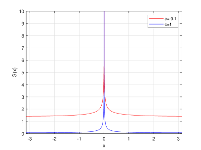
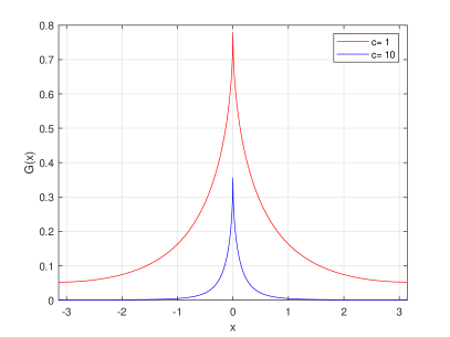
Figure 1. Profiles of $G_{\mathbb{T}}$ for $\alpha=0.5$ (left) and $\alpha=1.5$ (right) for specific values of $c$.

Green’s function $G_{\mathbb{R}}$ on the real line $\mathbb{R}$ is also used to understand interactions of strongly localized waves, e.g. attractive versus repelling interactions [16, 24] (see also [8, 29]). These interactions were recently studied in [10, 11] in the context of the beam equation, which corresponds to the case $\alpha=4$. The fractional cases for $\alpha\in(0,2)$ and $\alpha\in(2,4)$ are also important from applications in quantum computing, fluid dynamics, and elasticity theory.

Theorem 1 shows that the properties of $G_{\mathbb{T}}$ for $\alpha\in(0,2)$ are similar to those for $\alpha=2$ (the same holds for $G_{\mathbb{R}}$). However, it is an open question if the properties of $G_{\mathbb{T}}$ for $\alpha\in(2,4)$ are similar to those for $\alpha=4$, for which $G_{\mathbb{R}}$ has infinitely many oscillations, whereas the number of oscillations of $G_{\mathbb{T}}$ depends on $c>0$ and becomes infinite in the limit of $c\to\infty$ (see Appendix B). In the second part of this paper, we present numerical results which support the following conjecture.

Conjecture 1.

For each $\alpha\in(2,4]$, there exists $c_{0}>0$ such that for $c\in(0,c_{0})$, Green’s function $G_{\mathbb{T}}$ defined by (1.3) and (1.4) is even, strictly positive on $\mathbb{T}$, and monotonically decreasing on $(0,\pi)$. For $c\in[c_{0},\infty)$, $G_{\mathbb{T}}$ has a finite number of zeros on $\mathbb{T}$. The number of zeros is bounded in the limit of $c\to\infty$ if $\alpha\in(2,4)$ and unbounded as $c\to\infty$ if $\alpha=4$.

Since the limit $c\to\infty$ for Green’s function $G_{\mathbb{T}}$ can be rescaled as Green’s funciton $G_{\mathbb{R}}$ with $c$ normalized to unity, Conjecture 1 implies the following conjecture (relevant for interactions of strongly localized waves in [10, 11]).

Conjecture 2.

For every $c>0$ and every $\alpha\in(2,4]$, Green’s function $G_{\mathbb{R}}$ is not strictly positive on $\mathbb{R}$ and is not monotonically decreasing on $(0,\infty)$. It has a finite number of zeros on $\mathbb{R}$ if $\alpha\in(2,4)$ and an infinite number of zeros if $\alpha=4$.

Figure 2 illustrates the statement of Conjecture 1. For $\alpha=2.5$ (top), Green’s function $G$ has the single-lobe positive profile for $c=2$ (red curve) but it is not positive for $c=10$ (blue curve). For $\alpha=3.5$ (bottom), it is positive for $c=1$ (red curve), has one pair of zeros for $c=10$ (blue curve), and has two pairs of zeros for $c=60$ (black curve).

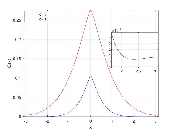
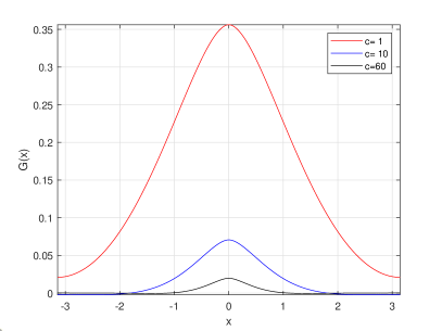
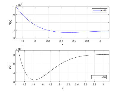
Figure 2. Profiles of $G$ on $\mathbb{T}$ for $\alpha=2.5$ (top) and $\alpha=3.5$ (bottom) at specific values of $c$.

The remainder of the article is structured as follow. Section 2 presents an overview of the Mittag-Leffler function and its properties. The integral representation of Green’s function $G_{\mathbb{T}}$ is derived in Section 3. The proof of Theorem 1 is presented in Section 4. The validity of Conjecture 1 is discussed in Section 5. Conclusion is given in Section 6. Appendices A and B give explicit formulas for Green’s function $G_{\mathbb{T}}$ for local cases of $\alpha=2$ and $\alpha=4$, respectively. Appendix C contains formal asymptotic results to support Conjecture 1 for $\alpha>2$ with small $|\alpha-2|$.

2. Properties of Mittag–Leffler function

Here we discuss properties of the Mittag–Leffler function defined by

$$E_{\alpha}(x)=\sum_{k=0}^{\infty}\frac{x^{k}}{\Gamma(k\alpha+1)},\qquad\alpha>0,$$ (2.1)

and its two-parametric generalization defined by

$$E_{\alpha,\beta}(x)=\sum_{k=0}^{\infty}\frac{x^{k}}{\Gamma(k\alpha+\beta)},\qquad\alpha,\beta>0.$$ (2.2)

Mittag–Leffler functions were introduced in the theory of analytic functions [25]. In recent years, they became popular due to their applications in fractional differential equations [20]. Indepth studies of the Mittag–Leffler functions can be found in [4] and [15].

Mittag–Leffler functions are typically used to represent solutions of initial-value problems for the fractional differential equations defined by the Riemann-Liouville or Caputo fractional derivatives [20]. As our study involves the boundary-value problem for the fractional Laplacian $(-\Delta)^{\alpha/2}$, Mittag–Leffler function $E_{\alpha}(-x^{\alpha})$ is used in the integral representation of Green’s function $G_{\mathbb{T}}$. This integral representation is derived in Section 3.

Here we review some important properties of the Mittag–Leffler functions.

Lemma 2.1.

For every $\alpha>0$ and every $x\in\operatorname{\mathbb{R}}$, it is true that

$$E_{\alpha,\alpha}(x)=\alpha\frac{d}{dx}E_{\alpha}(x).$$ (2.3)

Proof.

The result is obtained by differentiating (2.1) and using (2.2):

$$\frac{d}{dx}E_{\alpha}(x)=\sum_{k=1}^{\infty}\frac{x^{k-1}}{\alpha\Gamma(\alpha k)}=\frac{1}{\alpha}\sum_{k=0}^{\infty}\frac{x^{k}}{\Gamma(\alpha k+\alpha)}=\frac{1}{\alpha}E_{\alpha,\alpha}(x).$$

The series converges absolutely for every $x\in\mathbb{R}$ since $E_{\alpha}$ and $E_{\alpha,\alpha}$ are entire functions. ∎

Lemma 2.2.

[31] For every $\alpha\in(0,1]$, the function $x\mapsto E_{\alpha}(-x)$ is positive and completely monotonic for $x\geq 0$, that is

$$(-1)^{m}\frac{d^{m}}{dx^{m}}E_{\alpha}(-x)\geq 0,\qquad m\in\mathbb{N},\quad x\geq 0.$$ (2.4)

Consequently, $E_{\alpha,\alpha}(-x)\geq 0$ for every $x\geq 0$.

Remark 2.1.

A necessary and sufficent condition for the function $x\mapsto E_{\alpha}(-x)$ to be completely monotonic for $x\geq 0$ is that $E_{\alpha}(-x)$ can be expressed in the form

$$E_{\alpha}(-x)=\int_{0}^{\infty}e^{-xt}dF_{\alpha}(t),\quad x\geq 0,$$

where $F_{\alpha}$ is a nondecreasing and bounded on $(0,\infty)$. The proof of [31] is based on the representation of $E_{\alpha}(-x)$ given by

$$E_{\alpha}(-x)=\frac{1}{2i\pi\alpha}\int_{C}\frac{e^{t^{1/\alpha}}}{t+x}dt,$$

with a specially selected the contour $C$ in $\mathbb{C}$.

Lemma 2.3.

[15] For every $\alpha\in(0,2)$, $E_{\alpha}(-x^{\alpha})$ admits the asymptotic expansion

$$E_{\alpha}(-x^{\alpha})=-\sum_{k=1}^{N}\frac{(-1)^{k}}{\Gamma(1-\alpha k)x^{\alpha k}}+\mathcal{O}\left(\frac{1}{|x|^{\alpha N+\alpha}}\right)\quad\mbox{\rm as}\quad x\to\infty,$$ (2.5)

where $N\in\mathbb{N}$ is arbitrarily fixed. For every $\alpha\geq 2$, $E_{\alpha}(-x^{\alpha})$ admits the asymptotic expansion

$$E_{\alpha}(-x^{\alpha})=\frac{1}{\alpha}\sum_{n=-N+1}^{N}e^{a_{n}x}+\mathcal{O}\left(\frac{1}{|x|^{\alpha}}\right)\quad\mbox{\rm as}\quad x\to\infty,$$ (2.6)

where $a_{n}=e^{\frac{i\pi(2n-1)}{\alpha}}$ and $N$ is the largest integer satisfying the bound $2N-1\leq\frac{\alpha}{2}$.

Remark 2.2.

Asymptotic expansions (2.5) and (2.6) can be differentiated term by term.

Remark 2.3.

We list the explicit cases of the Mittag–Leffler function $E_{\alpha}(-x^{\alpha})$ for the first integers:

$$\alpha=1, \quad E_{1}(-x)=e^{-x},$$

$$\alpha=2, \quad E_{2}(-x^{2})=\cos(x),$$

$$\alpha=3, \quad E_{3}(-x^{3})=\frac{1}{3}e^{-x}+\frac{2}{3}\displaystyle{e^{\frac{x}{2}}}\cos\left(\frac{\sqrt{3}x}{2}\right),$$

$$\alpha=4, \quad E_{4}(-x^{4})=\cos\left(\frac{x}{\sqrt{2}}\right)\cosh\left(\frac{x}{\sqrt{2}}\right).$$

For $\alpha=1$, the asymptotic representation (2.5) admits zero leading-order terms for every $N\in\mathbb{N}$. The asymptotic representation (2.6) is also obvious from the exact expressions for $\alpha=2,3,4$, moreover, the remainder term is zero for $\alpha=2$ and can be included to the summation by increasing $N$ by one for $\alpha=3$ and $\alpha=4$.

Lemma 2.4.

[15] For every $\alpha\in(0,2)$ and every $x\in\operatorname{\mathbb{R}}$, $E_{\alpha}(-x)$ satisfies the following integral representation,

$$E_{\alpha}(-x^{\alpha})=\frac{2}{\pi}\sin\left(\frac{\pi\alpha}{2}\right)\int_{0}^{\infty}\frac{t^{\alpha-1}\cos(xt)}{1+2t^{\alpha}\cos\left(\frac{\pi\alpha}{2}\right)+t^{2\alpha}}dt.$$ (2.7)

Remark 2.4.

It is claimed in [15] that the integral representation (2.7) is true for all $\alpha>0$, however, the integral is singular for $\alpha=2$ and a discrepancy exists at $x=0$ for $\alpha>2$. For example, when $\alpha=3$, it follows from (2.1) that $E_{3}(0)=1$ whereas computing the integral given in (2.7) via the change of variable $u=t^{3}$ gives

$$E_{3}(0) =-\frac{2}{3\pi}\int_{0}^{\infty}\frac{du}{1+u^{2}}=-\frac{1}{3}\neq 1.$$

Hence, the integral representation (2.7) can only be used for $\alpha\in(0,2)$, for which $E_{\alpha}(-x^{\alpha})$ is bounded and decaying as $x\to+\infty$.

3. Integral representation of Green’s function $G_{\mathbb{T}}$

Here, we take Green’s function $G_{\mathbb{T}}$ defined by the Fourier series in (1.4) and rewrite it in the integral form involving the Mitag–Leffler function $E_{\alpha,\alpha}$. The following proposition gives the result for $\alpha\in(0,2]$.

Proposition 3.1.

For every $c>0$ and every $\alpha\in(0,2]$, it is true that

$$G_{\mathbb{T}}(x)=\frac{1}{2\pi c}+\frac{1}{\pi c}\int_{0}^{\infty}\left(\frac{e^{t}\cos(x)-1}{1-2e^{t}\cos(x)+e^{2t}}\right)t^{\alpha-1}E_{\alpha,\alpha}(-ct^{\alpha})dt,\quad x\in\mathbb{T}.$$ (3.1)

Proof.

Assume first that $x\neq 0$ and $c\in(0,1)$. Expanding each term of the trinometric sum in (1.4) into absolutely convergent geometric series and interchanging the two series, we obtain

$$\sum_{n=1}^{\infty}\frac{\cos(nx)}{c+n^{\alpha}}=\sum_{n=1}^{\infty}\frac{\cos(nx)}{n^{\alpha}}\sum_{k=0}^{\infty}\left(\frac{-c}{n^{\alpha}}\right)^{k}=\sum_{k=0}^{\infty}(-c)^{k}\sum_{n=1}^{\infty}\frac{\cos(nx)}{n^{\alpha(k+1)}}.$$ (3.2)

It is known from the integral representation (1) in [32, Section 5.4.2] that for every $x\neq 0$ and $\alpha>0$ that

$$\sum_{n=1}^{\infty}\frac{\cos(nx)}{n^{\alpha(k+1)}}=\frac{1}{\Gamma(\alpha k+\alpha)}\int_{0}^{\infty}\frac{t^{\alpha(k+1)-1}\left(e^{t}\cos(x)-1\right)}{1-2e^{t}\cos(x)+e^{2t}}dt,$$ (3.3)

where $k\geq 0$. Substituting (3.3) into (3.2) and interchanging formally the summation and the integration yields the following representation:

$$\sum_{n=1}^{\infty}\frac{\cos(nx)}{c+n^{\alpha}} =\sum_{k=0}^{\infty}\frac{(-c)^{k}}{\Gamma(\alpha k+\alpha)}\int_{0}^{\infty}\frac{t^{\alpha(k+1)-1}\left(e^{t}\cos(x)-1\right)}{1-2e^{t}\cos(x)+e^{2t}}dt,$$ (3.4)

$$=\int_{0}^{\infty}\left(\frac{e^{t}\cos(x)-1}{1-2e^{t}\cos(x)+e^{2t}}\right)t^{\alpha-1}\sum_{k=0}^{\infty}\frac{\left(-ct^{\alpha}\right)^{k}}{\Gamma(\alpha k+\alpha)}dt,$$ (3.5)

$$=\int_{0}^{\infty}\left(\frac{e^{t}\cos(x)-1}{1-2e^{t}\cos(x)+e^{2t}}\right)t^{\alpha-1}E_{\alpha,\alpha}(-ct^{\alpha})dt.$$ (3.6)

This yields formally the integral formula (3.1). Let us now justify the interchange of summation and integration in (3.4). Using the chain rule and Lemma 2.1, we get

$$t^{\alpha-1}E_{\alpha,\alpha}(-ct^{\alpha})=-\frac{1}{c}\frac{d}{dt}E_{\alpha}(-ct^{\alpha}).$$ (3.7)

It follows from (3.7) that for every $\alpha\in(0,2]$, the asymptotic expansion (2.5) in Lemma 2.3 for $\alpha\in(0,2)$ and Remark 2.3 for $\alpha=2$ imply that

$$\sup_{t\in[0,\infty)}t^{\alpha-1}|E_{\alpha,\alpha}(-t^{\alpha})|<\infty.$$ (3.8)

Hence, the integral in (3.1) converges absolutely for every $x\neq 0$ and $\alpha\in(0,2]$. Similarly, the integral in (3.4) converges absolutely for every $x\neq 0$ and $\alpha\in(0,2]$, whereas the numerical series converges absolutely for every $c\in(0,1)$. Thus, the interchange of summation and integration in (3.4) is justified by Fubini’s theorem.

For $x=0$, we note that $G_{\mathbb{T}}(0)<\infty$ if $\alpha>1$ and $G_{\mathbb{T}}(0)=\infty$ if $\alpha\in(0,1]$. Since $E_{\alpha,\alpha}(-x^{\alpha})=1+\mathcal{O}(x^{\alpha})$ as $x\to 0$, the integral in (3.1) converges absolutely for $x=0$ and $\alpha\in(1,2]$ and diverges for $x=0$ and $\alpha\in(0,1]$. Hence, the integral representation (3.1) holds again for $x=0$, $c\in(0,1)$, and $\alpha\in(0,2]$.

In order to extend the integral representation (3.1) from $c\in(0,1)$ to every $c>0$, we use real analyticity of Green’s function $G_{\mathbb{T}}$ and the integral in (3.1) in $c$ for $c>0$. Due to uniqueness of the analytical continuation of both $G_{\mathbb{T}}$ and the integral in (3.1) in $c$, the equality in (3.1) is uniquely continued from $c\in(0,1)$ to $c>0$. ∎

The integral representation (3.1) of Green’s function $G_{\mathbb{T}}$ can be justified for $\alpha>2$ provided that $c$ is sufficiently small. This result is described by the following proposition.

Proposition 3.2.

For every $\alpha>2$, there exists $c_{\alpha}>0$ given by

$$c_{\alpha}:=\left[\cos\left(\frac{\pi}{\alpha}\right)\right]^{-\alpha},$$ (3.9)

such that for every $c\in(0,c_{\alpha})$, the integral representation (3.1) is true for every $x\in\mathbb{T}$.

Proof.

The asymptotic expansion (2.6) in Lemma 2.3 implies for every $c>0$ and $\alpha>2$ that

$$\sup_{t\in[0,\infty)}e^{-t\cos\left(\frac{\pi}{\alpha}\right)}t^{\alpha-1}|E_{\alpha,\alpha}(-t^{\alpha})|<\infty,$$ (3.10)

where we have used again the connection formula (3.7). In addition, $E_{\alpha,\alpha}(-x^{\alpha})=1+\mathcal{O}(x^{\alpha})$ as $x\to 0$. Due to the above properties, the integral in (3.1) converges absolutely for every $x\in\mathbb{T}$ if $c\in(0,c_{\alpha})$, where $c_{\alpha}$ is given by (3.9). This justifies the formal computations in the proof of Proposition 3.1. ∎

Remark 3.1.

For $c\geq c_{\alpha}$ and $\alpha>2$, the Fourier series representation (1.4) suggests that $|G_{\mathbb{T}}(x)|<\infty$ for every $x\in\mathbb{T}$. However, the integral in (3.1) does not converge absolutely, hence it is not clear if the integral representation (3.1) can be used in this case. Our numerical results in Section 5 show that the integral representation (3.1) cannot be used for $c>c_{\alpha}$.

4. Green’s function $G_{\mathbb{T}}$ for $\alpha\in(0,2)$

Here, we prove Theorem 1 by using the integral representation (3.1) in terms of the Mittag–Leffler function $E_{\alpha,\alpha}$. It follows from (1.4) that $G_{\mathbb{T}}$ is even for every $c>0$ and $\alpha>0$. Furthermore, if $\alpha\in(0,1]$, then $\lim\limits_{x\to 0}G_{\mathbb{T}}(x)=+\infty$, and if $\alpha>1$, then

$$G_{\mathbb{T}}(0)=\frac{1}{2\pi}\left(\frac{1}{c}+2\sum_{n=1}^{\infty}\frac{1}{c+n^{\alpha}}\right)>0.$$

We shall prove that $G_{\mathbb{T}}^{\prime}(x)\leq 0$ for $x\in(0,\pi)$ and $G_{\mathbb{T}}(\pi)>0$ for every $c>0$ and $\alpha\in(0,2]$. For $\alpha=2$, this result follows from the exact analytical representation of $G_{\mathbb{T}}$ in Appendix A. Therefore, we focus on the case $\alpha\in(0,2)$ here. The following proposition gives an integral representation for $G_{\mathbb{T}}(\pi)$ which implies its strict positivity for every $c>0$ and $\alpha\in(0,2)$

Proposition 4.1.

For every $c>0$ and every $\alpha\in(0,2)$, it is true that

$$G_{\mathbb{T}}(\pi)=\frac{\sin(\frac{\alpha\pi}{2})}{\pi c^{1-\frac{1}{\alpha}}}\int_{0}^{\infty}\frac{s^{\alpha}\operatorname{csch}(\pi c^{\frac{1}{\alpha}}s)}{1+2s^{\alpha}\cos(\frac{\alpha\pi}{2})+s^{2\alpha}}ds,$$ (4.1)

which implies $G_{\mathbb{T}}(\pi)>0$.

Proof.

Evaluating the integral representation (3.1) at $x=\pi$, we obtain

$$G_{\mathbb{T}}(\pi)=\frac{1}{2\pi c}-\frac{1}{\pi c}\int_{0}^{\infty}\frac{1}{1+e^{t}}t^{\alpha-1}E_{\alpha,\alpha}(-ct^{\alpha})dt.$$ (4.2)

Substituting (3.7) into (4.2), integrating by parts, and using the asymptotic representation (2.5) to get zero contribution in the limit of $t\to\infty$, we obtain

$$G_{\mathbb{T}}(\pi)=\frac{1}{\pi c}\int_{0}^{\infty}\frac{e^{t}}{(1+e^{t})^{2}}E_{\alpha}(-ct^{\alpha})dt,$$ (4.3)

where the integral converges absolutely for every $c>0$ and $\alpha\in(0,2)$. Substituting the integral representation (2.7) for $E_{\alpha}(-ct^{\alpha})$ from Lemma 2.4 into (4.3), we obtain

$$G_{\mathbb{T}}(\pi)=\frac{2}{\pi^{2}c}\sin\left(\frac{\alpha\pi}{2}\right)\int_{0}^{\infty}\frac{e^{t}}{(1+e^{t})^{2}}\int_{0}^{\infty}\frac{s^{\alpha-1}\cos(c^{\frac{1}{\alpha}}ts)}{1+2s^{\alpha}\cos(\frac{\pi\alpha}{2})+s^{2\alpha}}dsdt.$$ (4.4)

Since both integrands belong to $L^{1}(0,\infty)$, the order of integration in (4.4) can be interchanged to get

$$G_{\mathbb{T}}(\pi)=\frac{2}{\pi^{2}c}\sin\left(\frac{\alpha\pi}{2}\right)\int_{0}^{\infty}\frac{s^{\alpha-1}}{1+2s^{\alpha}\cos(\frac{\pi\alpha}{2})+s^{2\alpha}}\int_{0}^{\infty}\frac{e^{t}\cos(c^{\frac{1}{\alpha}}st)}{(1+e^{t})^{2}}dtds.$$ (4.5)

The inner integral is evaluated exactly with the help of integral (7) in [32, Section 2.5.46]:

$$\int_{0}^{\infty}\frac{e^{t}\cos(c^{\frac{1}{\alpha}}st)}{(1+e^{t})^{2}}dt=\frac{\pi}{2}c^{\frac{1}{\alpha}}s\operatorname{csch}(\pi c^{\frac{1}{\alpha}}s),$$

When it is substituted into (4.5), it yields the integral representation (4.1). The integrand is positive and absolutely integrable for every $c>0$ and $\alpha\in(0,2)$, which implies that $G_{\mathbb{T}}(\pi)>0$. ∎

Remark 4.1.

Positivity of $G_{\mathbb{T}}(\pi)$ for $c>0$ and $\alpha\in(0,1]$ also follows from the representation (4.3) due to positivity of $E_{\alpha}(-ct^{\alpha})$ for every $t>0$ in Lemma 2.2. However, $E_{\alpha}(-ct^{\alpha})$ is not positive for all $t>0$ when $\alpha>1$, hence, the representation (4.3) is not sufficient for the proof of positivity of $G_{\mathbb{T}}(\pi)$ if $\alpha\in(1,2)$.

It remains to prove that $G_{\mathbb{T}}^{\prime}(x)\leq 0$ for every $x\in(0,\pi)$. The proof is carried differently for $\alpha\in(0,1]$ and for $\alpha\in(1,2)$. In the former case, we obtain the integral representation for $G_{\mathbb{T}}^{\prime}(x)$, which is strictly negative for $x\in(0,\pi)$. In the latter case, we employ the variational method to verify that the unique solution $G_{\mathbb{T}}$ of the boundary-value problem (1.3) admits the single lobe profile, with the only maximum located at the point of symmetry at $x=0$. The following two propositions give these two results.

Proposition 4.2.

For every $c>0$ and every $\alpha\in(0,1]$, $G_{\mathbb{T}}^{\prime}(x)<0$ for every $x\in(0,\pi)$.

Proof.

Differentiating the integral representation (3.1) in $x$ yields

$$G_{\mathbb{T}}^{\prime}(x) =\frac{1}{\pi c}\int_{0}^{\infty}t^{\alpha-1}E_{\alpha,\alpha}(-ct^{\alpha})\frac{d}{dx}\left(\frac{e^{t}\cos(x)-1}{1-2e^{t}\cos(x)+e^{2t}}\right)dt,$$

$$=-\frac{\sin(x)}{\pi c}\int_{0}^{\infty}t^{\alpha-1}E_{\alpha,\alpha}(-ct^{\alpha})\frac{e^{t}(e^{2t}-1)}{\left(1-2e^{t}\cos(x)+e^{2t}\right)^{2}}dt,$$ (4.6)

where the integrand is absolutely integrable. It follows by Lemma 2.2 that $E_{\alpha,\alpha}(-ct^{\alpha})\geq 0$ for $t>0$. Since $\sin(x)>0$ for $x\in(0,\pi)$, and the integrand is positive, it follows from the integral representation (4.6) that $G_{\mathbb{T}}^{\prime}(x)<0$ for $x\in(0,\pi)$. ∎

Proposition 4.3.

For every $c>0$ and every $\alpha\in(1,2)$, $G_{\mathbb{T}}^{\prime}(x)\leq 0$ for every $x\in(0,\pi)$.

Proof.

The proof consists of the following two steps. First, we obtain a variational solution to the boundary-value problem (1.3). Second, we use the fractional Polya–Szegö inequality to show that the solution $G_{\mathbb{T}}$ has a single-lobe profile on $\mathbb{T}$ with the only maximum located at the point of symmetry at $x=0$.

Step 1: Let us consider the following minimization problem,

$$\mathcal{B}_{c}:=\min_{u\in H^{\frac{\alpha}{2}}_{\rm per}(\mathbb{T})}\{B_{c}(u)-u(0)\},$$ (4.7)

where the quadratic functional $B_{c}(u)$ is given by

$$B_{c}(u)=\frac{1}{2}\int_{\mathbb{T}}\left[\left(D^{\frac{\alpha}{2}}u\right)^{2}+cu^{2}\right]dx.$$ (4.8)

Since $c>0$, we have

$$\frac{1}{2}\min(1,c)\|u\|_{H^{\frac{\alpha}{2}}_{\rm per}(\mathbb{T})} \leq B_{c}(u)\leq\frac{1}{2}\max(1,c)\|u\|_{H^{\frac{\alpha}{2}}_{\rm per}(\mathbb{T})},$$

hence, $B_{c}(u)$ is equivalent to the squared $H^{\frac{\alpha}{2}}_{\rm per}(\mathbb{T})$ norm. Moreover, for $\alpha\in(1,2)$, $\delta\in H^{-\frac{\alpha}{2}}_{\rm per}(\mathbb{T})$, the dual of $H^{\frac{\alpha}{2}}_{\rm per}(\mathbb{T})$ since

$$\|\delta\|_{H^{-\frac{\alpha}{2}}_{\rm per}(\mathbb{T})}=\sum_{\xi\in\mathbb{Z}}\frac{1}{\left(1+|\xi|^{2}\right)^{\frac{\alpha}{2}}}<\infty.$$

Thus, by Lax–Milgram theorem (see Corollary 5.8 in [5]), there exists a unique $G_{\mathbb{T}}\in H^{\frac{\alpha}{2}}_{\rm per}(\mathbb{T})$ such that $G_{\mathbb{T}}$ is the global minimizer of the variational problem (4.7), for which the Euler–Lagrange equation is equivalent to the boundary-value problem (1.3). By uniqueness of solutions of the two problems, $G_{\mathbb{T}}$ is equivalently written as the Fourier series (1.4), from which it follows that $G_{\mathbb{T}}(\pi)<G_{\mathbb{T}}(0)$. Hence, $G_{\mathbb{T}}$ is different from a constant function on $\mathbb{T}$.

Remark 4.2.

The variational method and in particular the Lax–Milgram theorem cannot be applied to the case $\alpha\in(0,1]$ since the Dirac delta distibution $\delta$ does not belong to the dual space of $H^{\frac{\alpha}{2}}_{\rm per}(\mathbb{T})$ when $\alpha\in(0,1]$.

Step 2: We utilize the fractional Polya–Szegö inequality, proved in the appendix of [9], to show that a symmetric decreasing rearrangement of the minimizer $G_{\mathbb{T}}$ on $\mathbb{T}$ does not increase $B_{c}(u)$. For completeness, we state the following definition and lemma.

Definition 4.1.

Let $m$ be the Lebesgue measure on $\mathbb{T}$ and $f(x):\operatorname{\mathbb{R}}\to\operatorname{\mathbb{R}}$ be a $2\pi$ periodic function. The symmetric and decreasing rearrangement $\tilde{f}$ of $f$ on $\mathbb{T}$ is given by

$$\tilde{f}(x)=\inf\{t:\;\;m(\{z\in\mathbb{T}:\;\;f(z)>t\})\leq 2|x|\},\hskip 14.45377ptx\in\mathbb{T}.$$ (4.9)

The rearrangement $\tilde{f}$ satisfies the following properties:

• $\tilde{f}(-x)=\tilde{f}(x)$ and $f^{\prime}(x)\leq 0$ for $x\in(0,\pi)$.

• $\tilde{f}(0)=\max_{x\in\mathbb{T}}f(x)$.

• $\|\tilde{f}\|_{L^{2}(\mathbb{T})}=\|f\|_{L^{2}(\mathbb{T})}$.

Lemma 4.1.

[9] For every $\alpha>1$ and every $f\in H^{\frac{\alpha}{2}}_{per}(\mathbb{T})$, it is true that

$$\int_{-\pi}^{\pi}|D^{\frac{\alpha}{2}}\tilde{f}|^{2}dx\leq\int_{-\pi}^{\pi}|D^{\frac{\alpha}{2}}f|^{2}dx.$$ (4.10)

The argument of the proof in the second step goes as follows. Suppose $\widetilde{G}_{\mathbb{T}}$ is the symmetric and decreasing rearrangement of $G_{\mathbb{T}}$, then by Lemma 4.1 and by property (iii) of Definition 4.9 we have $B_{c}(\widetilde{G}_{\mathbb{T}})\leq B_{c}(G_{\mathbb{T}})$. Since the global minimizer of the variational problem (4.7) is uniquely given by $G_{\mathbb{T}}$, $\widetilde{G}_{\mathbb{T}}$ coincides with $G_{\mathbb{T}}$ up to a translation on $\mathbb{T}$. However, it follows from (1.4) that $G_{\mathbb{T}}(-x)=G_{\mathbb{T}}(x)$ and $G_{\mathbb{T}}(\pi)<G_{\mathbb{T}}(0)$, hence an internal maximum at $x_{0}\in(0,\pi)$ would contradicts to the single-lobe profile of $G_{\mathbb{T}}$ and the only maximum of $G_{\mathbb{T}}$ is located at $0$, so that $G_{\mathbb{T}}(x)=\widetilde{G}_{\mathbb{T}}(x)$ for every $x\in\mathbb{T}$. It follows from property (i) of Definition 4.9 that $G_{\mathbb{T}}^{\prime}(x)\leq 0$ for $x\in(0,\pi)$. ∎

5. Green’s function $G_{\mathbb{T}}$ for $\alpha>2$

Here we provide numerical approximations of the Green’s function $G_{\mathbb{T}}$ for $\alpha>2$, which support Conjecture 1. The profiles of $G_{\mathbb{T}}$ are depicted on Figure 2. We only give details on how zeros of $G_{\mathbb{T}}(\pi)$ depend on parameters $(c,\alpha)$.

It follows from the Fourier series (1.4) that $G_{\mathbb{T}}(\pi)$ can be computed by the numerical series

$$G_{\mathbb{T}}(\pi)=\frac{1}{2\pi}\left(\frac{1}{c}+2\sum_{n=1}^{\infty}\frac{(-1)^{n}}{c+n^{\alpha}}\right),$$ (5.1)

where the series converges absolutely if $\alpha>1$. On the other hand, $G_{\mathbb{T}}(\pi)$ can also be computed from the integral representation (4.3), that is,

$$G_{\mathbb{T}}(\pi)=\frac{1}{\pi c}\int_{0}^{\infty}\frac{e^{t}}{(1+e^{t})^{2}}E_{\alpha}(-ct^{\alpha})dt,$$ (5.2)

which converges absolutely for $c\in(0,c_{\alpha})$, see Proposition 3.2, where $c_{\alpha}$ is given by (3.9).

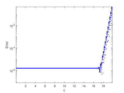
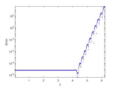
Figure 3. Difference between computations of $G_{\mathbb{T}}(\pi)$ in (5.1) and (5.2) for $\alpha=2.5$ (left) and $\alpha=3.5$ (right) versus parameter $c$.

Figure 3 shows the difference of $G_{\mathbb{T}}(\pi)$ computed from (5.1) and (5.2) for $\alpha=2.5$ (left) and $\alpha=3.5$ (right) in logarithmic scale versus parameter $c$. The Fourier series (5.1) is truncated such that the remainder is of the size $\mathcal{O}(10^{-10})$. For the integral representation of $G_{\mathbb{T}}(\pi)$ in (5.2), we numerically compute the Mittag–Leffler function $E_{\alpha}(-ct^{\alpha})$ on the half line; this task is accomplished by using the Matlab code provided in [14], where the Mittag-Leffler functions are approximated with relative errors of the size $\mathcal{O}(10^{-15})$. As follows from Fig. 3, the difference between the two computations is constantly small if $c<c_{\alpha}$, when the integral representation (5.2) converges absolutely, where $c_{\alpha=2.5}\approx 18.8$ and $c_{\alpha=3.5}\approx 5.2$. However, the accuracy of numerical computations based on the integral representation (5.2) deteriorates for $c$ approaching $c_{\alpha}$ and as a result, the difference between two computations quickly grows for $c>c_{\alpha}$.

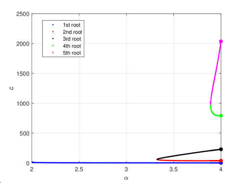
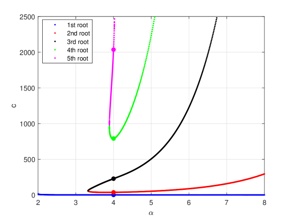
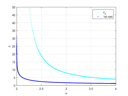
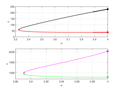
Figure 4. Top: Location of the first five roots of $G_{\mathbb{T}}(\pi)$ on the $(c,\alpha)$ plane. Bottom: The first root of $G_{\mathbb{T}}(\pi)$ relative to the boundary $c_{\alpha}$ (left). Coalescence of the 2nd and 3rd roots (upper right) and the 4th and 5th roots (lower right).

Roots of $G_{\mathbb{T}}(\pi)$ in $c$ for each fixed $\alpha>2$ are computed from the Fourier series representation (5.1) using the bisection method. Figure 4 (top) shows the first five zeros of $G_{\mathbb{T}}(\pi)$ on the $(c,\alpha)$ plane, where the dots show the roots of $G_{\mathbb{T}}(\pi)$ computed from the exact solutions in Appendix B for $\alpha=4$. The first root exists for every $\alpha>2$ and is located inside $(0,c_{\alpha})$, see the bottom left panel. The other roots are located outside $(0,c_{\alpha})$ and disappear via pairwise coalescence as $\alpha$ is reduced towards $\alpha=2$, see the bottom right panels. The 2nd and 3rd roots coalesce at $\alpha\approx 3.325$ and the 4th and 5th roots coalesce at $\alpha\approx 3.89$. The number of terms in the Fourier series of $G_{\mathbb{T}}(\pi)$ is increased to compute the 4th and 5th roots such that the remainder is of the size of $\mathcal{O}(10^{-14})$ because $G_{\mathbb{T}}(\pi)$ becomes very small near the location of these roots.

Table 1 compares the error between the numerically detected roots at $\alpha=4$ and the roots of $G_{\mathbb{T}}(\pi)$ obtained from solving the transcendental equation (B.7) in Appendix B.

Root	Error
1st	1.9915 e-11
2nd	7.1495 e-08
3rd	3.3182 e-06
4th	0.0031
5th	0.0156

Table 1. Difference between locations of the first five roots of $G_{\mathbb{T}}(\pi)$ for $\alpha=4$ computed from (5.1) and (B.7).

Green’s function $G_{\mathbb{T}}$ was computed versus $x$ using the Fourier series representation (1.4) for fixed values of $(c,\alpha)$. The plots of $G_{\mathbb{T}}$ are shown in Figures 1 and 2. Since the first root of $G_{\mathbb{T}}(\pi)$ occurs at $c\approx 2.507$ for $\alpha=2.5$ and at $c\approx 1.446$ for $\alpha=3.5$, see Fig. 4 (bottom left panel), the threshold $c_{0}$ in Conjecture 1 reduces with the larger value of $\alpha$. Appendix C gives a formal asymptotic approximation of the threshold $c_{0}$ as $\alpha\to 2$.

6. Conclusion

The main contribution of this work is the novel relation between Green’s function for the linear operator $c+(-\Delta)^{\alpha/2}$ on the periodic domain $\mathbb{T}$ and the Mittag–Leffler function. With the help of this relation, we have proved that Green’s funciton is strictly positive on $\mathbb{T}$ and single-lobe (monotonically decreasing away from the maximum point) for every $c>0$ and $\alpha\in(0,2]$. The same property is also true for sufficiently small $c$ and $\alpha\in(2,4]$ but we give numerical and asymptotic results that Green’s function has a finite number of zeros on $\mathbb{T}$ for sufficiently large $c$, the number of zeros is bounded in the limit $c\to\infty$ for $\alpha\in(2,4)$ but is unbounded for $\alpha=4$. Rigorous proof of properties of Green’s function for $\alpha\in(2,4)$ is an open problem left for further studies.

Appendix A Green’s function $G_{\mathbb{T}}$ for $\alpha=2$

Here we derive the exact analytic form of Green’s function $G_{\mathbb{T}}$ for $\alpha=2$. The following proposition reproduces Theorem 1 for $\alpha=2$.

Proposition A.1.

For every $c>0$, Green’s function $G_{\mathbb{T}}$ at $\alpha=2$ is even, strictly positive on $\mathbb{T}$, and strictly monotonically decreasing on $(0,\pi)$.

Proof.

For $\alpha=2$, Green’s function $G_{\mathbb{T}}$ satisfies the second-order differential equation

$$-G_{\mathbb{T}}^{\prime\prime}(x)+cG_{\mathbb{T}}(x)=\delta(x),\quad x\in\mathbb{T},$$ (A.1)

where $c>0$. It follows from the theory of Dirac delta distributions that $G_{\mathbb{T}}$ is continuous, even, periodic on $\mathbb{T}$, and have a jump discontinuity of the first derivative at $x=0$.

To see the jump condition of $G_{\mathbb{T}}^{\prime}(x)$ across $x=0$, we integrate (A.1) on $(-\varepsilon,\varepsilon)$ and then take the limit as $\varepsilon\to 0$.

$$\lim\limits_{\varepsilon\to 0}\int_{-\varepsilon}^{\varepsilon}\left(-G_{\mathbb{T}}^{\prime\prime}(x)+cG_{\mathbb{T}}(x)\right)dx=\lim\limits_{\varepsilon\to 0}\int_{-\varepsilon}^{\varepsilon}\delta(x)dx=1,$$ (A.2)

where the last equality follows from properties of $\delta$. Since $G_{\mathbb{T}}\in C^{0}(\mathbb{R})$, the second term on the left hand side vanishes as $\varepsilon\to 0$, which yields $-G_{\mathbb{T}}^{\prime}(0^{+})+G_{\mathbb{T}}^{\prime}(0^{-})=1$. Since $G_{\mathbb{T}}$ is even on $\mathbb{R}$, we obtain

$$G_{\mathbb{T}}^{\prime}(0^{+})=-\frac{1}{2}.$$ (A.3)

Additionally, it follows from the Fourier series representation (1.4) with $\alpha=2$ that

$$G_{\mathbb{T}}(0)=\frac{1}{2\pi}\sum_{n\in\mathbb{Z}}\frac{1}{c+n^{2}}=\frac{\coth(\sqrt{c}\pi)}{2\sqrt{c}},$$ (A.4)

where we have used numerical series (4) in [32, Section 5.1.25].

The differential equation (A.1) is solved for even $G_{\mathbb{T}}$ as follows:

$$G_{\mathbb{T}}(x)=G_{\mathbb{T}}(0)\cosh(\sqrt{c}x)+G_{\mathbb{T}}^{\prime}(0^{+})\frac{\sinh(\sqrt{c}|x|)}{\sqrt{c}},\quad x\in\mathbb{T}.$$

Due to (A.3) and (A.4), this can be rewritten in the closed form as

$$G_{\mathbb{T}}(x)=\frac{\cosh(\sqrt{c}(\pi-|x|))}{2\sqrt{c}\sinh(\sqrt{c}\pi)},\quad x\in\mathbb{T}.$$ (A.5)

It follows from (A.5) that

$$G_{\mathbb{T}}^{\prime}(x)=-\frac{\sinh(\sqrt{c}(\pi-x))}{2\sinh(\sqrt{c}\pi)}<0,\quad x\in(0,\pi),$$ (A.6)

and hence $G_{\mathbb{T}}$ is strictly monotonically decreasing on $(0,\pi)$. On the other hand,

$$G_{\mathbb{T}}(\pi)=\frac{1}{2\sinh(\sqrt{c}\pi)}>0,\quad c>0,$$ (A.7)

and hence $G_{\mathbb{T}}$ is strictly positive on $\mathbb{T}$. Note that the exact expression for $G_{\mathbb{T}}(\pi)$ in (A.7) also follows from numerical series (6) in [32, Section 5.1.25]. ∎

Remark A.1.

It follows from (A.5) that $G_{\mathbb{T}}^{\prime}(\pi)=0$, due to smoothness and periodicity of even $G_{\mathbb{T}}(x)$ across $x=\pm\pi$. Therefore, the exact expression in (A.5) and the relation for $G_{\mathbb{T}}(0)$ in (A.4) can be alternatively found by solving the differential equation (A.1) for even $G_{\mathbb{T}}$ subject to the boundary conditions $G_{\mathbb{T}}^{\prime}(0^{\pm})=\mp\frac{1}{2}$ and $G_{\mathbb{T}}^{\prime}(\pm\pi)=0$.

Appendix B Green’s function $G_{\mathbb{T}}$ for $\alpha=4$

Here we derive the exact analytic form of Green’s function $G_{\mathbb{T}}$ for $\alpha=4$. The following proposition proves Conjecture 1 for $\alpha=4$.

Proposition B.1.

There exists $c_{0}>0$ such that for $c\in(0,c_{0})$, Green’s function $G_{\mathbb{T}}$ at $\alpha=4$ is even, strictly positive on $\mathbb{T}$, and strictly monotonically decreasing on $(0,\pi)$. For $c\in[c_{0},\infty)$, $G_{\mathbb{T}}$ has a finite number of zeros on $\mathbb{T}$, which becomes unbounded as $c\to\infty$.

Proof.

For $\alpha=4$, Green’s function $G_{\mathbb{T}}$ satisfies the fourth-order differential equation

$$G_{\mathbb{T}}^{\prime\prime\prime\prime}(x)+cG_{\mathbb{T}}(x)=\delta(x),\quad x\in\mathbb{T},$$ (B.1)

where $c>0$. It follows from the theory of Dirac delta distributions that $G_{\mathbb{T}}$ is continuous, even, periodic on $\mathbb{T}$, and have a jump discontinuity of the third derivative at $x=0$. Similarly to the computation in (A.2), it follows that Green’s function solves the boundary-value problem with the boundary conditions

$$G_{\mathbb{T}}^{\prime}(0)=G_{\mathbb{T}}^{\prime}(\pm\pi)=G_{\mathbb{T}}^{\prime\prime\prime}(\pm\pi)=0,\quad G_{\mathbb{T}}^{\prime\prime\prime}(0^{\pm})=\pm\frac{1}{2}.$$ (B.2)

Due to the boundary conditions (B.2), it is easier to solve the differential equation (B.1) for $G_{\mathbb{T}}^{\prime}$ on $[0,\pi]$. By using the parametrization $c=4a^{4}$, we obtain

$$G_{\mathbb{T}}^{\prime}(x) = c_{1}\cosh(ax)\cos(ax)+c_{2}\cosh(ax)\sin(ax)$$

$$+c_{3}\sinh(ax)\cos(ax)+c_{4}\sinh(ax)\sin(ax),\quad x\in[0,\pi],$$

where $c_{1}$, $c_{2}$, $c_{3}$, and $c_{4}$ are some coefficients. We can find $c_{1}=0$ and $c_{4}=\frac{1}{4a^{2}}$ from the two boundary conditions (B.2) at $x=0^{+}$. The other two boundary conditions (B.2) at $x=\pi$ gives the linear system for $c_{2}$ and $c_{3}$:

$$\begin{bmatrix}\cosh(\pi a)\sin(\pi a)&\sinh(\pi a)\cos(\pi a)\\ \sinh(\pi a)\cos(\pi a)&-\cosh(\pi a)\sin(\pi a)\end{bmatrix}\begin{bmatrix}c_{2}\\ c_{3}\end{bmatrix}=-c_{4}\begin{bmatrix}\sinh(\pi a)\sin(\pi a)\\ \cosh(\pi a)\cos(\pi a)\end{bmatrix}.$$

By Cramer’s rule, we find the unique solution

$$c_{2}=-c_{4}\frac{\sinh(2\pi a)}{\cosh(2\pi a)-\cos(2\pi a)},\quad c_{3}=c_{4}\frac{\sin(2\pi a)}{\cosh(2\pi a)-\cos(2\pi a)},$$

which results in the exact analytical expression

$$G_{\mathbb{T}}^{\prime}(x)=\frac{1}{4a^{2}}\frac{\sinh(ax)\sin a(2\pi-x)-\sin(ax)\sinh a(2\pi-x)}{\cosh(2\pi a)-\cos(2\pi a)},\quad x\in[0,\pi].$$ (B.3)

Integrating (B.3) in $x$ yields the exact analytical expression for $G_{\mathbb{T}}$:

$$G_{\mathbb{T}}(x)=\frac{1}{8a^{3}}\frac{g(x)}{\cosh(2\pi a)-\cos(2\pi a)},\quad x\in[0,\pi],$$ (B.4)

where

$$g(x) := \sinh(ax)\cos a(2\pi-x)+\cosh(ax)\sin a(2\pi-x)$$

$$+\sin(ax)\cosh a(2\pi-x)+\cos(ax)\sinh a(2\pi-x)$$

and the constant of integration is set to zero due to the differential equation (B.1).

We verify the validity of the exact solution (B.4) by comparing $G_{\mathbb{T}}(0)$ and $G_{\mathbb{T}}(\pi)$ with the Fourier series representation (1.4) for $\alpha=4$:

$$G_{\mathbb{T}}(0)=\frac{1}{2\pi}\sum_{n\in\mathbb{Z}}\frac{1}{4a^{4}+n^{2}}=\frac{1}{8a^{3}}\frac{\sinh(2\pi a)+\sin(2\pi a)}{\cosh(2\pi a)-\cos(2\pi a)}$$ (B.5)

and

$$G_{\mathbb{T}}(\pi)=\frac{1}{2\pi}\sum_{n\in\mathbb{Z}}\frac{(-1)^{n}}{4a^{4}+n^{2}}=\frac{1}{4a^{3}}\frac{\sinh(\pi a)\cos(\pi a)+\sin(\pi a)\cosh(\pi a)}{\cosh(2\pi a)-\cos(2\pi a)}.$$ (B.6)

Indeed, the exact expressions coincide with those found from the numerical series (1) and (2) in [32, Section 5.1.27].

It follows from (B.6) that $G_{\mathbb{T}}(\pi)$ vanishes for $c=4a^{4}>0$ if and only if $a>0$ is a solution of the transcendental equation

$$\tanh(\pi a)+\tan(\pi a)=0.$$ (B.7)

Elementary graphical analysis on Figure 5 shows that there exist a countable sequence of zeros $\{a_{n}\}_{n\in\mathbb{N}}$ such that $a_{n}\in\left(n-\frac{1}{4},n\right)$, $n\in\mathbb{N}$. Hence, $G_{\mathbb{T}}$ is not positive for $a\in(a_{1},\infty)$.

Figure 5. Countable sequence of zeros $\{a_{n}\}_{n\in\mathbb{N}}$ of B.7

Let us now show that the profile of $G_{\mathbb{T}}$ is strictly, monotonically decreasing on $(0,\pi)$ for small $a$. It follows from (B.3) that $G_{\mathbb{T}}^{\prime}(x)<0$ for $x\in(0,\pi)$ if and only if

$$\frac{\sin(ax)}{\sinh(ax)}>\frac{\sin a(2\pi-x)}{\sinh a(2\pi-x)},\qquad x\in(0,\pi).$$ (B.8)

The function

$$x\mapsto\frac{\sin(ax)}{\sinh(ax)}$$

is monotonically decreasing on $[0,2\pi]$ as long as

$$\cos(ax)\sinh(ax)-\sin(ax)\cosh(ax)\leq 0,\qquad x\in[0,2\pi],$$ (B.9)

which is true at least for $a\in(0,\frac{1}{2})$. Hence, $G_{\mathbb{T}}$ is strictly motonically decreasing on $(0,\pi)$ with $G_{\mathbb{T}}(\pi)>0$ for $a\in(0,a_{0})$, where $a_{0}\in(\frac{1}{2},1)$. On the other hand, it is obvious that there exists $a_{*}\in(1,\frac{3}{2})$ such that the inequality (B.9) [and hence the inequality (B.8)] is violated at $x=\pi$ for $a\in(a_{*},2)$, for which $G_{\mathbb{T}}^{\prime}(x)>0$ at least near $x=\pi$.

The first part of the proposition is proven due to the relation $c=4a^{4}$. It remains to prove that $G_{\mathbb{T}}$ has a finite number of zeros on $\mathbb{T}$ for fixed $a\in[a_{0},\infty)$ which becomes unbounded as $a\to\infty$. To do so, we simplify the expression (B.4) for $G_{\mathbb{T}}$ in the asymptotic limit of large $a$ for every fixed $x\in(0,\pi)$:

$$G_{\mathbb{T}}(x)=\frac{1}{8a^{3}}\left[e^{-ax}\cos(ax)+e^{-ax}\sin(ax)+\mathcal{O}(e^{-a(2\pi-x)})\right]\quad\mbox{\rm as}\quad a\to\infty.$$ (B.10)

Thus, as $a$ gets large, there are finitely many zeros of $G_{\mathbb{T}}$ on $(0,\pi)$ but the number of zeros of $G_{\mathbb{T}}$ grows unbounded as $a\to\infty$. ∎

Remark B.1.

The leading-order term in the asymptotic expansion (B.10) represents Green’s function $G_{\mathbb{R}}$. The proof of Conjecture 2 for $\alpha=4$ follows from this explicit expression.

Remark B.2.

Figure 6 shows boundaries on the $(a,x)$ plane between positive (yellow) and negative (blue) values of $G_{\mathbb{T}}$ (left) and $G_{\mathbb{T}}^{\prime}$ (right). It follows from the figure that the zeros of $G_{\mathbb{T}}$ and $G_{\mathbb{T}}^{\prime}$ are monotonically decreasing with respect to parameter $a$ and the number of zeros only grows as $a$ increases. In other words, zeros of $G_{\mathbb{T}}$ cannot coalesce and disappear. We were not able to prove these properties for every $a>0$ inside $(0,\pi)$ (however, the proof can be given at $x=\pi$).

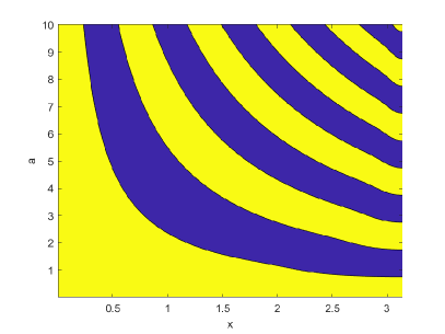
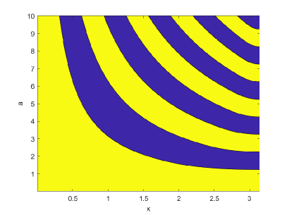
Figure 6. Left: areas on $(a,x)$ plane where $G_{\mathbb{T}}$ is positive (yellow) and negative (blue). Right: the same but for $G_{\mathbb{T}}^{\prime}$.

Appendix C Asymptotic approximation of the first zero of $G_{\mathbb{T}}(\pi)$

Here, we obtain the formal asymptotic dependence of the first zero of $G_{\mathbb{T}}(\pi)$ as $(c,\alpha)\to(\infty,2)$. We use the integral representation (5.2). Replacing the Mittag–Leffler function $E_{\alpha}$ by its leading-order asymptotic expression (2.6) for $2\leq\alpha<6$, we obtain formally

$$G_{\mathbb{T}}(\pi)=\frac{1}{2\pi\alpha c}\left[I(a,b)+\mbox{\rm error terms}\right],$$ (C.1)

where

$$I(a,b):=\int_{0}^{\infty}{\rm sech}^{2}\left(\frac{t}{2}\right)e^{at}\cos(bt)dt$$ (C.2)

with

$$a:=c^{\frac{1}{\alpha}}\cos\left(\frac{\pi}{\alpha}\right),\quad b:=c^{\frac{1}{\alpha}}\sin\left(\frac{\pi}{\alpha}\right).$$ (C.3)

The limit $(c,\alpha)\to(\infty,2)$ such that $c<c_{\alpha}$ corresponds to the limit $b\to\infty$ with $a<1$.

The integral $I(a,b)$ is the rapidly oscillating integral in the limit $b\to\infty$. We split it into two parts:

$$I(a,b) = I_{1}(a,b)+I_{2}(a,b)\qquad\qquad$$ (C.4)

$$= \int_{0}^{\infty}{\rm sech}^{2}\left(\frac{t}{2}\right)\cosh(at)\cos(bt)dt+\int_{0}^{\infty}{\rm sech}^{2}\left(\frac{t}{2}\right)\sinh(at)\cos(bt)dt,$$

where $I_{1}(a,b)$ is exponentially small in $b$ and $I_{2}(a,b)$ is algebraically small in $b$. Indeed, by Darboux principle [1], we evaluate the first integral for $a<1$ with the residue theorem:

$$I_{1}(a,b) =\frac{1}{2}{\rm Re}\int_{-\infty}^{\infty}{\rm sech^{2}}\left(\frac{t}{2}\right)\cosh(at)e^{ibt}dt\qquad\qquad\qquad\qquad\qquad\qquad$$

$$={\rm Re}4\pi i{\rm Res}_{z=\pi i}\left[\frac{e^{z}\cosh(az)e^{ibz}}{(1+e^{z})^{2}}\right]+\mathcal{O}(e^{-3\pi b})$$

$$=4\pi\left[b\cos(\pi a)+a\sin(\pi a)\right]e^{-\pi b}+\mathcal{O}(e^{-3\pi b}).$$

Integrating the second integral by parts several times for $a<1$ (see Section 5.2 in [21]), we obtain

$$I_{2}(a,b) =\frac{1}{b}\sin(bt)\sinh(at){\rm sech}^{2}\left(\frac{t}{2}\right)\biggr{|}_{t=0}^{t\to\infty}-\frac{1}{b}\int_{0}^{\infty}\sin(bt)\frac{d}{dt}\left[{\rm sech}^{2}\left(\frac{t}{2}\right)\sinh(at)\right]dt\qquad\qquad\qquad\qquad\qquad\qquad$$

$$=\frac{\cos(bt)}{b^{2}}\frac{d}{dt}\left[{\rm sech}^{2}\left(\frac{t}{2}\right)\sinh(at)\right]\biggr{|}_{t=0}^{t\to\infty}-\frac{1}{b^{2}}\int_{0}^{\infty}\cos(bt)\frac{d^{2}}{dt^{2}}\left[{\rm sech}^{2}\left(\frac{t}{2}\right)\sinh(at)\right]dt$$

$$=-\frac{a}{b^{2}}+\mathcal{O}\left(\frac{a}{b^{4}}\right).$$

Finding zero of $I(a,b)$ in $a$ as $b\to\infty$ yields the approximation

$$a=4\pi b^{3}e^{-\pi b}\left[1+\mathcal{O}\left(\frac{1}{b^{2}}\right)\right].$$ (C.5)

Substituting (C.3) into (C.5) then taking the logarithm of both sides yields the following transcendental equation for $c^{\frac{1}{\alpha}}$

$$2\ln\left(c^{\frac{1}{\alpha}}\right)-\pi\sin\left(\frac{\pi}{\alpha}\right)c^{\frac{1}{\alpha}}+\mathcal{O}(c^{-\frac{2}{\alpha}})=\ln\left(\frac{\cos(\frac{\pi}{\alpha})}{4\pi\sin^{3}\left(\frac{\pi}{\alpha}\right)}\right).$$ (C.6)

In order to determine the dependence of $c$ in terms of $\alpha$ we first factor $c^{\frac{1}{\alpha}}$ on the left hand side, then expand around $\alpha=2$ to obtain

$$-\pi c^{\frac{1}{\alpha}}\left[1+\mathcal{O}\left((\alpha-2)^{2}\right)+\mathcal{O}\left(\frac{\ln\left(c^{\frac{1}{\alpha}}\right)}{c^{\frac{1}{\alpha}}}\right)\right]=\ln\left[\frac{\alpha-2}{16}+\mathcal{O}\left((\alpha-2)^{2}\right)\right].$$

Since $c^{\frac{1}{\alpha}}$ is of order $\mathcal{O}(\ln(\alpha-2))$, the above equation becomes

$$-\pi c^{\frac{1}{\alpha}}=\ln\left(\frac{\alpha-2}{16}\right)\left[1+\mathcal{O}\left(\frac{\ln|\ln(\alpha-2)|}{|\ln(\alpha-2)|}\right)\right],$$

which, as $\alpha\to 2$, implies

$$c=\frac{1}{\pi^{2}}\ln^{2}\left(\frac{\alpha-2}{16}\right)\left[1+\mathcal{O}\left(\frac{\ln|\ln(\alpha-2)|}{|\ln(\alpha-2)|}\right)\right].$$ (C.7)

The asymptotic approximation (C.7) suggests that the first zero of $G_{\mathbb{T}}(\pi)$ at $c=c_{0}(\alpha)$ satisfies $c_{0}(\alpha)\to\infty$ as $\alpha\to 2$. However, we note that the asymptotic approximation of the root of $I(a,b)$ given by (C.7) is derived without analysis of the error terms in (C.1).

References

- [1] J. Boyd, Chebyshev and Fourier Spectral Methods (Dover Publishers, New York, 2001).
- [2] V. Ambrosio, “On the existence of periodic solutions for a fractional Schrödinger equation”, Proc. AMS 146 (2018), 3767–3775.
- [3] Z. Bai and H. Lü, “Positive solutions for boundary value problem of nonlinear fractional differential equation”, J. Math. Anal. Appl. 311 (2005), 495–505.
- [4] H. Bateman, Higher Transcendental Functions. Vol. III (McGraw-Hill Book Company, New York, 1953).
- [5] H. Brezis, Functional Analysis, Sobolev Spaces and Partial Differental Equations (Springer, New York, 2011).
- [6] H. Chen, “Existence of periodic traveling-wave solutions of nonlinear, dispersive wave equations”, Nonlinearity 17 (2004), 2041–2056.
- [7] H. Chen and J. Bona, “Periodic travelling wave solutions of nonlinear dispersive evolution equations”, Discr. Cont. Dynam. Syst. 33 (2013), 4841–4873.
- [8] M. Chugunova and D.E. Pelinovsky, “Two-pulse solutions in the fifth-order KdV equation: rigorous theory and numerical approximations”, Discr. Cont. Dynam. Syst. B 8 (2007), 773–800.
- [9] K. Claasen, M. Johnson, “Nondegeneracy and Stability of antiperiodic bound states for fractional nonlinear Schrödinger equations”, J. Diff. Equs. 266 (2019), 5664–5712
- [10] R.J. Decker, A. Demirkaya, N.S. Manton, and P.G. Kevrekidis, “Kink-antikink interaction forces and bound states in a biharmonic model”, arXiv:2001.06973 (2020).
- [11] R.J. Decker, A. Demirkaya, P.G. Kevrekidis, D. Iglesias, J. Severino, and Y. Shavit, “Kink dynamics in a nonlinear beam model”, arXiv:2005.04523 (2020).
- [12] Z. Du and C. Gui, “Further study on periodic solutions of elliptic equations with a fractional Laplacian”, Nonlinear Analysis 193 (2020) 111417 (16 pages)
- [13] R.L. Frank and E. Lenzmann, “Uniqueness of non-linear ground states for fractional Laplacian in ”, Acta Math. 210 (2013), 261–318.
- [14] R. Garappa, The Mittag–Leffler function (https://www.mathworks.com/matlabcentral/fileexchange/48154-the-mittag-leffler-function), MATLAB Central File Exchange. Retrieved October 31, 2020.
- [15] R. Gorenflo, A. Kilbas, F. Mainardi, and S. Rogosin. Mittag–Leffler Functions, Related Topics and Applications (Springer-Verlag, Berlin, 2014).
- [16] K.A. Gorshkov and L.A. Ostrovsky, “Interactions of solitons in nonintegrable systems: Direct perturbation method and applications”, Physica D 3 (1981), 428–438.
- [17] S. Hakkaev and A.G. Stefanov, “Stability of periodic waves for the fractional KdV and NLS equations”, arXiv: 1907.05149 (2019).
- [18] V.M. Hur and M. Johnson, “Stability of periodic traveling waves for nonlinear dispersive equations”, SIAM J. Math. Anal. 47 (2015), 3528–3554.
- [19] M.A. Johnson, “Stability of small periodic waves in fractional KdV-type equations”, SIAM J. Math. Anal. 45 (2013), 3168–3293.
- [20] A. A. Kilbas, H. M. Srivastava, J. J. Trujillo, Theory and Application of Fractional Differential Equations North-Holland Mathematics Studies 204 (Elsevier, New York, 2006).
- [21] F. Olver. Asymptotics and Special Functions (AKP Classics, Massachusetts, 1996).
- [22] U. Le, D. Pelinovsky, “Convergence of Petviashvili’s Method Near Periodic Waves In The Fractional Kortweg-De Vries Equation”, SIAM J. Math. Anal. 51 (2019), 2850–2883.
- [23] A. Lischke, G. Pang, M. Gulian, F. Song, C. Glusa, X. Zheng, Z. Mao, W. Cai, M.M. Meerschaert, M. Ainsworth, and G.E. Karniadakis, “What is the fractional Laplacian? A comparative review with new results”, J. Comp. Phys. 404 (2020), 109009 (62 pages).
- [24] N.S. Manton, “An effective Lagrangian for solitons”, Nucl. Phys. B 150 (1979), 397-412.
- [25] M.G Mittag- Leffler, “Sur la nouvelle fonction ”, Acad. Sci. Paris 137 (1903), 554–558.
- [26] F. Natali, D. Pelinovsky and U. Le, “New variational characterization of periodic waves in the fractional Korteweg–de Vries equation”, Nonlinearity 33 (2020), 1956–1986.
- [27] F. Natali, D. Pelinovsky and U. Le, “Periodic waves in the fractional modified Korteweg–de Vries equation”, arXiv (2020).
- [28] J. J. Nieto, Maximum principles for fractional differential equations derived from Mittag–Leffler functions, Appl. Math. Lett. 23 (2010), 1248–1251.
- [29] R. Parker and B. Sandstede, “Periodic multi-pulses and spectral stability in Hamiltonian PDEs with symmetry”, arXiv: 2010: 05728 (2021)
- [30] I. Podlubny, Fractional Differential Equations, Mathematics in Science and Engineering 198 (Academic Press, California, 1998)
- [31] H. Pollard, “The complete monotonic character of the Mittag–Leffler function ”, Bull. Amer. Math. Soc. 54 (1948), 1115–1116.
- [32] A. P. Prudnikov, Y. A. Brychkov, and O. I. Marichev, Integrals and Series: Volume 1–Elementary Functions. (N.M. Queen Trans), (Taylor & Francis, London, 2002).
- [33] L. Roncal and P.R. Stinga, “Fractional Laplacian on the torus”, Commun. Contemp. Math. 18 (2016), 1550033 (26 pages).