Adjoint SU(5) GUT model with Modular $S_{4}$ Symmetry

Abstract

We study the textures of SM fermion mass matrices and their mixings in a supersymmetric adjoint SU(5) Grand Unified Theory with modular $S_{4}$ being the horizontal symmetry. The Yukawa entries of both quarks and leptons are expressed by modular forms with lower weights. Neutrino sector has an adjoint SU(5) representation 24 as matter superfield, which is a triplet of $S_{4}$. The effective light neutrino masses is generated through Type-III and Type-I seesaw mechanism. The only common complex parameter in both charged fermion and neutrino sectors is modulus $\tau$. Down-type quarks and charged leptons have the same joint effective operators with adjoint scalar in them, and their mass discrepancy in the same generation depends on Clebsch-Gordan factor. Especially for the first two generations the respective Clebsch-Gordan factors made the double Yukawa ratio $y_{d}y_{\mu}/y_{e}y_{s}=12$, in excellent agreement with the experimental result. We reproduce proper CKM mixing parameters and all nine Yukawa eigenvalues of quarks and charged leptons. Neutrino masses and MNS parameters are also produced properly with normal ordering is preferred.

1 Introduction

Despite of great success, especially the discovery of Higgs boson [1, 2], the standard model (SM) still has some problems unsolved in particle physics. One of the problems is the origin of flavor structure for the SM fermions, which mainly refers to the enormous mass difference among different generations, and distinct mixing patterns between lepton and quark sector.

The masses of charged fermions, from lightest electron of MeV level to heaviest top quark being 173GeV, span almost 5 orders of magnitude. The situation becomes even worse when the neutrino sector is contained, since the neutrino masses of sub-eV are nearly 7 orders of magnitude smaller than that of electron. Besides the absolute mass scale and mass ordering are still yet to be determined by future high-precision neutrino experiments. Apart from the large mass hierarchy, quark CKM parameters manifest a mixing pattern of small angles [3]. However the situation is completely different in lepton MNS mixing matrix. The precise neutrino oscillation data has provided us a picture of two large angles $\theta_{12}$ and $\theta_{23}$, and one small angle $\theta_{13}$, which is comparable with the quark Cabibbo angle $\theta_{C}$.

It is an unsolved puzzle to interpret the observed flavor structure in quark and lepton sector. The flavor parameters, include all the fermion masses, mixing angles as well as CP violating phases arise from the dependence of Yukawa on flavor. Since symmetry plays an important role in physics, it is worth to constrain the Yukawa interactions with the supervision of flavor symmetry, hence the mass hierarchies and mixing patterns of SM fermions could be interpreted by the additional symmetry beyond the gauge symmetry of the SM. But note that flavor symmetry is not the unique top-down scenario to understand the flavor structure. The other possible top-down approaches include, such as anarchy [4], extra dimension [5, 6] and string theory [7, 8, 9].

For the last two decades, the precise measurement of flavor parameters, especially that of lepton mixing angles, has motivated the model building by using discrete symmetry group to elucidate the different flavor structures between quarks and leptons. Non-Abelian discrete groups, such as lower order groups $A_{4}$, $A_{5}$, $S_{4}$ and other ones with higher order, are wildly used in such kind of works. And it is indeed easy to reproduce at least the two large leptonic mixing angles. For reviews see Refs. [10, 11, 12, 13, 14, 15]. In the models apart from the essential Higgs, some extra scalar fields called flavons are introduced. They are singlets under SM gauge group but have nontrivial representations under flavor group, whose vacuum orientation in flavor space can induce specific Yukawa textures for fermions. In neutrino sector the famous Tri-Bimaximal mixing [16, 17] is ubiquitous in many realistic models.

Non-Abelian discrete groups as flavor symmetries are success in explaining the leptonic mixing pattern with large angles, with the price of introducing a number of gauge singlets called flavon fields in conventional studies. The flavor symmetry is broken when the scalar flavons acquiring vacuum expectation values (VEV) by non-trivial dynamical way. Such VEVs with specific configurations control the flavor textures of fermions and thus a few of free coupling parameters appear in the Yukawa entries. Besides the values of VEVs themselves are determined by some other parameters. The more parameters in the traditional flavor models, the less predictive power they have. And the fermion masses are still often acquired by tuning the coupling parameters, even though the VEVs of the flavons can be nearly fixed such that all the couplings can be naturally of the same order, e.g., of order one.

Recently the modular symmetry provides another possibility to interpret the flavor issues [18]. The simplest modular symmetry implementation only demands one complex field, called modulus $\tau$, as the unique source of modular symmetry breaking when it develops a VEV, hence the vacuum configuration problem is greatly simplified. In such a simplest framework the Yukawa couplings are just modular forms which are the holomorphic functions of modulus $\tau$, then the flavon fields are not indispensable ingredient for model building, and thus tremendously reduce the amount of particle content and the free parameters of the theory.

The modular invariance models are based on the level $N$ finite modular group $\Gamma_{N}$, e.g., from $N=2$ to 5, $\Gamma_{2}\simeq S_{3}$  [19, 20, 21, 22], $\Gamma_{3}\simeq A_{4}$  [18, 23, 24, 25, 29, 30, 28, 26, 27, 32, 31, 33, 34], $\Gamma_{4}\simeq S_{4}$  [35, 36, 37, 38, 39, 40, 41, 42, 43] and $\Gamma_{5}\simeq A_{5}$  [44, 45, 41], which are all inhomogeneous modular groups. In such models the Yukawa couplings are weight $k$ modular forms with $k$ being even numbers. Most of the studies focus on the lepton flavor issues, while few of them include quark sector  [24, 20, 31, 25]. The unified quark and lepton models can be implemented in the context of SU(5) grand unified theories (GUT) combined with the modular symmetries [32, 21]. Besides the topics on the fermion flavor structures, the related phenomenological issues has been discussed in those works, such as the dark matter models [27], baryon number violation [26] and leptogenesis  [33, 34, 22]. On the other side, the double covering of finite modular group which is homogeneous, has been used as flavor symmetry as well  [46, 47, 48, 49, 50, 51].

Motivated by the phenomenological viable mass ratios between quarks and leptons, and the idea of Yukawa couplings can be modular forms, in the study we combine the modular flavor symmetry $\Gamma_{4}\simeq S_{4}$ with the supersymmetric adjoint SU(5) GUT [52] to forge the flavor textures of quarks and leptons simultaneously. In refs. [32, 21] the neutrino masses are generated via type-I  [53, 54, 55, 56] seesaw by adding at least two gauge singlets, i.e., right-handed heavy neutrinos. However there exist another two possibilities in SU(5) GUT to produce light neutrino masses: first is type-II seesaw mechanism  [57, 58, 59] by adding an extra Higgs $\textbf{15}_{H}$, and second is Type-I plus Type-III [60] seesaw by adding fermionic field in the 24 dimensional representation. The two cases in SU(5) GUT have not been explored yet in the recent modular flavor models. In this paper we explore for the first time the second scheme to produce effective light neutrino masses. Meanwhile we would like to give rise to a realistic Yukawa ratios between charged leptons and down-quarks. The Yukawa ratio in each generation is directly derived from the novel Clebsch-Gordan (CG) factor, which can be comparable to the phenomenological values at GUT scale. For the modular flavor model built on SU(5) GUT, the flavon-free model is such that the double Yukawa eigenvalue ratio $y_{\mu}y_{d}/y_{e}y_{s}$ equal to 12 for the first and second families of charged leptons and down quarks. The other viable cases which can generate the acceptable ratios, however, still require the flavon or so called weighton to compensate the loss of mass dimension.

There is no flavon but a modulus $\tau$ in the modular symmetry breaking sector, meanwhile the gauge symmetry is broken by one adjoint scalar $H_{24}$. We aim at minimizing the amount of free coupling parameters in the unified model. For higher weight modular forms, it will bring more free coupling parameters, and thus decrease the predictive power of the model. Thus we use lower weight modular forms to give the modular invariant operators.

In order to achieve the above goal, we should strictly contrain the representations and weights under $S_{4}$ for the fields. To be specific, all the 10-dimensional matter superfields are $S_{4}$ singlets and have distinct weights. The three families of $\bar{\textbf{5}}$s are divided into an doublet and a singlet but have the same weight. At last the 24 fermionic superfields are sealed in a triplet. For the scalar sector, the $\textbf{5}_{H}$, $\textbf{45}_{H}$ and $\textbf{24}_{H}$ are just singlets with distinct weights. Please see Table. 1 for details.

In quark and charged lepton sector the Yukawa matrices are very sparse with several texture zeros. The adjoint scalar $H_{24}$ couples to the matter superfields in down quark sector, then it induces the novel ratio of CG factors 1/2 and 6 for the first two families of leptons and down quarks, and 3/2 for the third one. In neutrino sector we introduce the 24 dimensional matter field rather than a gauge singlet to produce the neutrino masses through Type-I and Type-III seesaw mechanism. Since we introduce the adjoint matter fields rather than gauge singlets to produce the effective masses of light neutrinos, the Yukawa matrices are slightly different for the heavy $\rho_{3}$ and $\rho_{0}$ in the 24. And the same for Majorana mass matrices, since the mass terms include two nontrivial couplings: the pure mass term which is the same for $\rho_{3}$ and $\rho_{0}$, and the new interaction between 24 and $H_{24}$, which splits the masses of $\rho_{3}$ and $\rho_{0}$. Such new interaction is of course absent in the models which gauge singlets are responsible for seesaw mechanism.

The layout of the paper is arranged as follows. In Sec. 2 we introduce the framework for the model building work, including the brief review on modular group, especially the one with level $N=4$, $\Gamma_{4}\simeq S_{4}$ and the modular forms of weight 2 and 4. Then we give the basic aspects of adjoint SU(5) GUT. In Sec. 3 we present the flavor model based on adjoint SU(5) GUT combined with modular $S_{4}$ flavor symmetry. We show that the GUT flavor model can be built without introducing a gauge singlet scalar. The entries of Yukawa matrices of quarks and charged leptons have only modular forms in them. In Sec. 4, we first give the convention for Yukawa matrices and the SUSY threshold corrections, then we present the data to be used and perform the numerical fit to the Yukawa matrices with threshold effects included. Sec. 5 devotes to the summary of the study.

2 The Framework

In the section we shall briefly discuss the framework and environment used for the construction of model. First we give a brief review on the basic concepts of modular symmetry with lower level $N$ and modular forms of weight $k$. The finite modular group $\Gamma_{4}$ is used for our model building work, so we give the modular forms with weight $k=2,4$. Secondly we introduce the basic aspects of adjoint SU(5) grand unified theory, including the matter multiplets and scalar Higgs together with the vacuum configurations of the scalars.

2.1 Modular group and Modular forms

The modular group $\overline{\Gamma}$ implies the linear fractional transformations $\gamma$ that act on the complex $\tau$ in the upper-half complex plane

$$\tau\rightarrow\gamma\tau=\frac{a\tau+b}{c\tau+d},\quad a,b,c,d\in\mathbb{Z},\quad ad-bc=1,\quad\textrm{Im}\tau>0,$$ (1)

The generators $S$ and $T$ are the two transformations satisfying

$$S^{2}=(ST)^{3}=\mathbb{I},$$ (2)

with the representation matrices as

$$S=\left(\begin{array}[]{cc}0&1\\ -1&0\\ \end{array}\right),\quad T=\left(\begin{array}[]{cc}1&1\\ 0&1\\ \end{array}\right),$$ (3)

lead to

$$S:\tau\rightarrow-\frac{1}{\tau},\quad T:\tau\rightarrow\tau+1.$$ (4)

We introduce the series of infinite normal subgroups $\Gamma(N)$, $N=1,2,3,\cdots$ of $SL(2,\mathbb{Z})$

$$\Gamma(N)=\Bigg{\{}\left(\begin{array}[]{cc}a&b\\ c&d\\ \end{array}\right)\in SL(2,\mathbb{Z}),\quad\left(\begin{array}[]{cc}a&b\\ c&d\\ \end{array}\right)=\left(\begin{array}[]{cc}1&0\\ 0&1\\ \end{array}\right)(\textrm{mod}\;N)\Bigg{\}}.$$ (5)

For $N=1,2$ we define $\overline{\Gamma}(N)=\Gamma(N)/\{\mathbb{I},-\mathbb{I}\}$ and for $N>2$ we have $\overline{\Gamma}(N)=\Gamma(N)$. Taking the quotient $\Gamma_{N}\equiv\overline{\Gamma}/\overline{\Gamma}(N)$, one can obtain a finite subgroup called finite modular group. Especially for $N\leq 5$ the groups $\Gamma_{N}$ are isomorphic to the permutation groups $\Gamma_{2}\simeq S_{3},\Gamma_{3}\simeq A_{4},\Gamma_{4}\simeq S_{4}$ and $\Gamma_{5}\simeq A_{5}$, which are ubiquitous in the construction of flavor models.

Modular forms $f(\tau)$ of weight $k$ and level $N$ are holomorphic functions transforming under the groups $\Gamma(N)$ in the way as

$$f(\gamma\tau)=(c\tau+d)^{k}f(\tau),\quad\gamma\in\Gamma(N).$$ (6)

Here $k$ is even number, and $N$ is natural. Given the weight $k$ and level $N$, the modular forms span a linear space of dimension equals to $k+1$. The basis in the linear space can be chosed such that the modular form $f_{i}(\tau)$ in a multiplet transforms according to a unitary representation $\rho$ of the group $\Gamma_{N}$:

$$f_{i}(\gamma\tau)=(c\tau+d)^{k}\rho(\gamma)_{ij}f_{j}(\tau),\qquad\gamma\in\Gamma_{N}.$$ (7)

In the study we take $N=4$ as the case of interest and construct an explicit grand unified flavor model to elucidate the fermion masses and mixings. In the case of lowest weight 2, there are 5 linear independent modular forms. These modular forms are explicitly expressed in terms of Dedekind eta-function $\eta(\tau)$:

$$\eta(\tau)=q^{1/24}\prod^{\infty}_{n=1}(1-q^{n}),\qquad q=e^{i2\pi\tau}.$$ (8)

To be specific, the modular forms are defined as the functions of $\eta(\tau)$ and its derivatives of the form

$$Y(c_{1},\cdots,c_{6}|\tau)\equiv c_{1}\frac{\eta^{\prime}(\tau+\frac{1}{2})}{\eta(\tau+\frac{1}{2})}+c_{2}\frac{\eta^{\prime}(4\tau)}{\eta(4\tau)}+c_{3}\frac{\eta^{\prime}(\frac{\tau}{4})}{\eta(\frac{\tau}{4})}+c_{4}\frac{\eta^{\prime}(\frac{\tau+1}{4})}{\eta(\frac{\tau+1}{4})}+c_{5}\frac{\eta^{\prime}(\frac{\tau+2}{4})}{\eta(\frac{\tau+2}{4})}+c_{6}\frac{\eta^{\prime}(\frac{\tau+3}{4})}{\eta(\frac{\tau+3}{4})},$$ (9)

with the coefficients $c_{1}+\cdots+c_{6}=0$. For the case of weight 2, the basis is comprised of five modular forms as follow:

$$Y_{1}(\tau)\equiv Y(1,1,\omega,\omega^{2},\omega,\omega^{2}|\tau),$$ (10)

$$Y_{2}(\tau)\equiv Y(1,1,\omega^{2},\omega,\omega^{2},\omega|\tau),$$ (11)

$$Y_{3}(\tau)\equiv Y(1,-1,-1,-1,1,1|\tau),$$ (12)

$$Y_{4}(\tau)\equiv Y(1,-1,-\omega^{2},-\omega,\omega^{2},\omega|\tau),$$ (13)

$$Y_{5}(\tau)\equiv Y(1,-1,-\omega,-\omega^{2},\omega,\omega^{2}|\tau),$$ (14)

with $\omega\equiv e^{2\pi i/3}$. The modular forms $(Y_{1},Y_{2})^{T}$ and $(Y_{3},Y_{4},Y_{5})^{T}$ transform as an doublet and triplet of $S_{4}$ respectively, i.e., they are denoted as

$$Y_{\bf{2}}(\tau)\equiv\left(\begin{array}[]{c}Y_{1}(\tau)\\ Y_{2}(\tau)\\ \end{array}\right),\quad Y_{\bf{3}^{\prime}}(\tau)\equiv\left(\begin{array}[]{c}Y_{3}(\tau)\\ Y_{4}(\tau)\\ Y_{5}(\tau)\\ \end{array}\right).$$ (15)

One can get modular forms of higher weights from the tensor productions of weight 2 modular forms, and thus obtain different irreps of $S_{4}$. Taking weight $k=4$ for example, we then have 9 independent modular forms, and they are arranged into the following singlets and multiplets irreps of $S_{4}$

$$Y^{(4)}_{\bf{1}}=Y_{1}Y_{2},\quad Y^{(4)}_{\bf{2}}=\left(\begin{array}[]{c}Y^{2}_{2}\\ Y^{2}_{1}\\ \end{array}\right),$$ (18)

$$Y^{(4)}_{\bf{3}}=\left(\begin{array}[]{c}Y_{1}Y_{4}-Y_{2}Y_{5}\\ Y_{1}Y_{5}-Y_{2}Y_{3}\\ Y_{1}Y_{3}-Y_{2}Y_{4}\\ \end{array}\right),\quad Y^{(4)}_{\bf{3}^{\prime}}=\left(\begin{array}[]{c}Y_{1}Y_{4}+Y_{2}Y_{5}\\ Y_{1}Y_{5}+Y_{2}Y_{3}\\ Y_{1}Y_{3}+Y_{2}Y_{4}\\ \end{array}\right).$$ (25)

We use the above modular forms of weight 2 and 4 to construct our modular invariant model in Sec. 3. For higher weight modular forms, one may refer to Ref. [36] for further information.

2.2 Basic aspects of Adjoint SU(5)

In this part we shall give the fermion sector and the scalars used for the model setup. According to the distinct representations under the gauge symmetry, the matter fields are divided into the following three parts: anti-fundamental $\bar{\textbf{5}}$, anti-symmetrical tensor 10 and the adjoint 24. We assume the usual three generations of $\bar{\textbf{5}}$ and 10, which have the decomposition under the SM gauge group $SU(3)_{C}\otimes SU(2)_{L}\otimes U(1)_{Y}$. The theory of renormalizable adjoint SU(5) can be seen in ref. [61]. Concerning our model, we promote the matter fields to superfields in Minimal Supersymmetry Standard Model (MSSM) and embed them into SU(5) representations $\bar{\textbf{5}}$ and 10. For $\bar{\textbf{5}}$ we denote

$$\qquad F_{i}=(d^{c}_{R}\quad d^{c}_{B}\quad d^{c}_{G}\quad e\quad-\nu)_{i}=d^{c}_{i}\oplus\ell_{i}$$ (26)

and for 10

$$\qquad T_{i}=\frac{1}{\sqrt{2}}\left(\begin{array}[]{ccccc}0&-u^{c}_{G}&u^{c}_{B}&-u_{R}&-d_{R}\\ u^{c}_{G}&0&-u^{c}_{R}&-u_{B}&-d_{B}\\ -u^{c}_{B}&u^{c}_{R}&0&-u_{G}&-d_{G}\\ u_{R}&u_{B}&u_{G}&0&-e^{c}\\ d_{R}&d_{B}&d_{G}&e^{c}&0\\ \end{array}\right)_{i}=u^{c}_{i}\oplus q_{i}\oplus e^{c}_{i},$$ (27)

where $i=1,2,3$ indicates the family indices of standard model (SM), and $R,B,G$ stand for the color indices. The adjoint matter field 24 reads

$$\textbf{24}=\frac{1}{\sqrt{2}}\left(\begin{array}[]{cc}\frac{1}{\sqrt{2}}\boldsymbol{\lambda}.\boldsymbol{\rho}_{8}-\sqrt{\frac{2}{15}}\rho_{0}&\rho_{(3,2)}\\ \rho_{(\bar{3},2)}&\frac{1}{\sqrt{2}}\boldsymbol{\sigma}.\boldsymbol{\rho}_{3}+\sqrt{\frac{3}{10}}\rho_{0}\\ \end{array}\right),$$ (28)

in which $\lambda^{i}$ are the Gell-Mann matrices. The scalar fields contain the following Higgs fields

$$\textbf{5}_{H}=T_{(3,1)}\oplus H_{1},$$ (29)

$$\textbf{45}_{H}=S_{8}\oplus S_{(\bar{6},1)}\oplus S_{(3,3)}\oplus S_{(\bar{3},2)}\oplus S_{(3,1)}\oplus S_{(\bar{3},1)}\oplus H_{2},$$

$$\textbf{24}_{H}=\Sigma_{8}\oplus\Sigma_{3}\oplus\Sigma_{(3,2)}\oplus\Sigma_{(\bar{3},2)}\oplus\Sigma_{24}.$$

The VEVs of the scalars are listed as the follwing form

$$\langle\textbf{5}_{H}\rangle=\frac{v_{5}}{\sqrt{2}}(0,0,0,0,1)^{T},$$ (32)

$$\langle\textbf{24}_{H}\rangle=v_{24}\textrm{diag}(1,1,1,-3/2,-3/2),$$

$$\langle\textbf{45}_{H}\rangle^{i5}_{j}=\frac{v_{45}}{\sqrt{2}}[\textrm{diag}(1,1,1,-3,0)]^{i}_{j},\quad\langle\textbf{45}_{H}\rangle^{in}_{j}=0,$$

where $i,j=1,...,5$, $n=1,...,4$ and $v=\sqrt{|v_{5}|^{2}+24|v_{45}|^{2}}=246\textrm{GeV}$.

3 Adjoint SU(5) GUT Flavor Model

Now let us present the supersymmetric adjoint SU(5) GUT flavor model in details. First we assign the representations and weights of chiral supermultiplets. For sake of simplicity we shall impose certain constraints on the assignments. For matter fields, three generations of $\bf{10}$ dimensional representations, denoted by $T_{1,2,3}$, are all $S_{4}$ singlets, i.e., $\rho_{T_{i}}\sim\bf{1}$, $(i=1,2,3)$, but have distinct weights for each family. The first two generations of $\bf{\bar{5}}$ dimensional representations, named as $F_{1,2}$, are assigned to be a doublet of $S_{4}$, i.e., $F=(F_{1},F_{2})$, while the third generation $F_{3}$ is a $S_{4}$ singlet. Nevertheless the three $\bf{\bar{5}}$s have the same weight. In addition to the 10- and $\bar{\textbf{5}}$-dimensional representations in SU(5) GUTs, the adjoint $\bf{24}$ dimensional matter superfields $A$ have also three families, and they are assigned to be an triplet of $S_{4}$, denoted by $A=(A_{1},A_{2},A_{3})$.

For the Higgs sector $H_{5}$, $H_{45}$, $H_{\bar{5}}$ and $H_{\overline{45}}$ are responsible for the electroweak symmetry broken, while the GUT gauge group is broken by an adjoint scalar field $H_{24}$. We shall not intend to explain the mass hierarchy of charged fermions, which is beyond the power of modular symmetry. And in order to made the coupling terms minimality, we do not introduce any flavon fields like conventional models did. Instead all the Yukawa couplings are modular forms with specific weights to ensure the modular invariance. The only modular symmetry breaking source arises from the modulus $\tau$ developing its VEV. For simplicity the modular weights are assigned such that the Yukawa couplings have as lower weights as possible. The representations and weights of the chiral supermultiplets are listed in the Table 1.

Table 1: Field content and their representation assignments under the gauge group SU(5), modular $S_{4}$ and their weights $k_{I}$ in the model.

Fields	$T_{1}$	$T_{2}$	$T_{3}$	$F=(F_{1},F_{2})$	$F_{3}$	$A$	$H_{5}$	$H_{\bar{5}}$	$H_{45}$	$H_{\overline{45}}$	$H_{24}$
$SU(5)$	$\bf{10}$	$\bf{10}$	$\bf{10}$	$\bf{\bar{5}}$	$\bf{\bar{5}}$	$\bf{24}$	$\bf{5}$	$\bf{\bar{5}}$	$\bf{45}$	$\overline{\bf{45}}$	$\bf{24}$
$\Gamma_{4}\equiv S_{4}$	$\bf{1}$	$\bf{1}$	$\bf{1}$	$\bf{2}$	$\bf{1}$	$\bf{3}^{\prime}$	$\bf{1}$	$\bf{1}^{\prime}$	$\bf{1}$	$\bf{1}$	$\bf{1}^{\prime}$
$k_{I}$	0	$-1$	1	1	1	$-1$	$-2$	1	0	$-1$	$-2$

3.1 SU(5) breaking

For the purpose of our model construction, we start with SU(5) breaking superpotential. Since we have only one adjoint scalar field $H_{24}$ in the model, the gauge symmetry broken into SM gauge group is realized by the adjoint scalar acquiring the vacuum expectation value of $H_{24}$. The SU(5) breaking superpotential is simply as

$$\mathcal{W}_{24}=M_{24}Y^{(4)}_{\textbf{1}}\textrm{Tr}H^{2}_{24}+\lambda Y^{(6)}_{\textbf{1}^{\prime}}\textrm{Tr}H^{3}_{24},$$ (33)

then one can get the VEV of $H_{24}$, i.e., $\langle H_{24}\rangle$ in eq. (32) with

$$v_{24}=\frac{4M_{24}Y^{(4)}_{\textbf{1}}}{3\lambda_{1}Y^{(6)}_{\textbf{1}^{\prime}}}.$$ (34)

Besides causing the GUT breaking, the adjoint scalar field $H_{24}$ would also couple to the matter fields leading to novel Clebsch-Gordan factors, and especially the exotic Yukawa coupling ratios between down quark sector and charged lepton sector at GUT scale. See the next section for details.

3.2 Charged Fermions

In this section we will present the Yukawa couplings for charged fermions. Since the flavons are not an essential part of the model, the relevant Yukawa coupling terms in up-type quark sector manifest in renormalisable level, while those in down-type quarks and charged lepton sector show in effective operators. Since the quarks have enormous mass hierarchies but small mixing angles, the resulting Yukawa matrices should be controllable in the entries. A practical viable scheme is to induce texture zeros for Yukawa matrices. And another keypoint is the GUT-scale Yukawa ratios between leptons and down-quarks have to fulfil certain phenomenological constraints from experiments as well.

The Yukawa coupling terms for up quarks in superpotential involve two Higgs fields, i.e., $H_{5}$ and $H_{45}$. Because of the symmetry constraints only the following couplings are allowed

$$\mathcal{W}_{u}=\alpha_{u}T_{1}T_{1}H_{45}+\beta_{u}T_{2}T_{2}H_{5}Y^{(4)}_{\bf{1}}+\gamma_{u}T_{3}T_{3}H_{5}+g_{u}T_{2}T_{3}H_{45},$$ (35)

which leads to a block diagonal mass matrix

$$M_{u}=\left[\begin{array}[]{ccc}\alpha_{u}v_{45}&0&0\\ 0&\beta_{u}Y_{1}Y_{2}v_{5}&g_{u}v_{45}\\ 0&-g_{u}v_{45}&\gamma_{u}v_{5}\\ \end{array}\right].$$ (36)

The operators of dimension 4, such as those in Eq. (35), are expressed by the diagram in Figure. 1  , in which the dashed line stands for scalar Higgs and solid lines are matter multiplets. In Table 2 we give the list of dimension 4 operators corresponding to Figure. 1 including those in the next sections.

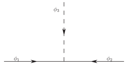
Figure 1: The supergraph for dimension 4 operators.

Field	1	2	3	4	5	6	7	8
$\phi_{1}$	$T_{1}$	$T_{2}$	$T_{3}$	$T_{2}$	$T_{1}$	F	$F_{3}$	A
$\phi_{2}$	$T_{1}$	$T_{2}$	$T_{3}$	$T_{3}$	$F_{3}$	A	A	A
$\phi_{3}$	$H_{45}$	$H_{5}$	$H_{5}$	$H_{45}$	$H_{\overline{45}}$	$H_{5}$	$H_{5}$	$H_{24}$

Table 2: The list for dimension 4 operators corresponding to Figure. 1.

In SU(5) GUTs, the left and right handed components of up-type quarks reside in the same representations $T_{i}$, that is why the Yukawa couplings are of the form $T_{i}T_{j}H_{s}$ ($s=5,45$) which made the Yukawa elements either symmetric or antisymmetric. However those of down-type quarks live in different representations: $F_{i}$ includes the right handed component and $T_{i}$ has left handed quark doublet. And vice verse for charged leptons. Then the interactions of both down quarks and charged leptons are written by the same joint operators of the form $T_{i}F_{j}H_{\bar{s}}$. Accordingly the corresponding Yukawa couplings, $Y_{d}$ and $Y_{e}$, are just mutual transposed relation up to $\mathcal{O}(1)$ CG factors. Therefore the eigenvalues have to satisfy certain phenomenological GUT relations. For the first two families, the following double Yukawa ratio[64]

$$\frac{y_{\mu}}{y_{s}}(\frac{y_{e}}{y_{d}})^{-1}=10.7^{+1.8}_{-0.8},$$ (37)

is a strong restriction on model building. Besides the Yukawa eigenvalues in both up and down quarks sectors, the quark mixing CKM parameters have to be fulfil as well. All the requirements imply that only certain CG factors can be realistic in GUT flavor models. To be specific, in our model the effective superpotential in down quarks sector and charged leptons sector is written by the operators

$$\mathcal{W}_{d}=\frac{\alpha_{d}}{\Lambda}[T_{1}H_{\overline{45}}]_{45}[FH_{24}]_{\overline{45}}Y_{\bf{2}}+\frac{\beta_{d}}{\Lambda}[T_{2}H_{24}]_{10}[FH_{\bar{5}}]_{\overline{10}}Y_{\bf{2}}+\frac{\gamma_{d}}{\Lambda}[T_{3}H_{\bar{5}}]_{5}[F_{3}H_{24}]_{\bar{5}}+g_{d}T_{1}F_{3}H_{\overline{45}},$$ (38)

where the SU(5) contraction $[XY]_{R}$ of fields $X$ and $Y$ denotes a tensor in the representation $R$. Here the adjoint scalar $H_{24}$ is crucial to form the dimension five operators which result the new Yukawa ratios between leptons and quarks. After the GUT gauge symmetry is broken when $H_{24}$ develops its VEV along the hypercharge direction, the Clebsch-Gordan factors emerge in the entries of lepton and quark Yukawa matrices. These SU(5) tensor contractions are realized by integrating out heavy messengers. The effective operators in the superpotential are then generated, see Figure. 2. For the model to work, we list the messenger fields and their representations as well as weights in Table 3.

We define the quantity $\epsilon=\langle H_{24}\rangle/\Lambda$, then the mass matrix of down-type quarks reads

$$M_{d}=\left[\begin{array}[]{ccc}\alpha_{d}v_{\overline{45}}\epsilon Y_{2}&-\alpha_{d}v_{\overline{45}}\epsilon Y_{1}&g_{d}v_{\overline{45}}\\ \beta_{d}v_{\bar{5}}\epsilon Y_{2}&\beta_{d}v_{\bar{5}}\epsilon Y_{1}&0\\ 0&0&\gamma_{d}v_{\bar{5}}\epsilon\\ \end{array}\right],$$ (39)

and that of charged leptons is simply the transposed $M_{d}$ up to the CG coefficients of Yukawa couplings

$$M_{e}=\left[\begin{array}[]{ccc}C_{1}\alpha_{d}v_{\overline{45}}\epsilon Y_{2}&C_{2}\beta_{d}v_{\bar{5}}\epsilon Y_{2}&0\\ -C_{1}\alpha_{d}v_{\overline{45}}\epsilon Y_{1}&C_{2}\beta_{d}v_{\bar{5}}\epsilon Y_{1}&0\\ C_{4}g_{d}v_{\overline{45}}&0&C_{3}\gamma_{d}v_{\bar{5}}\epsilon\\ \end{array}\right],$$ (40)

The CG coefficients in the model are $C_{1}=-1/2$, $C_{2}=6$, $C_{3}=-3/2$ and $C_{4}=-3$. Note that the fourth CG factor is the famous Georgi-Jarlskog relation  [65]. The first three ones are the main predictions for the mass relations between quarks and leptons, which can be realized in conventional models, such as [66, 67]. We can check that the double ratio in Eq. (37) is satisfied for the present choice. The set of the CG coefficients, $C_{1}=-1/2$ and $C_{2}=6$, is in fact the only one that can be realized in GUT without flavons. The other two possibilities in realistic flavor GUT models, e.g., (A) $C_{1}=4/9,C_{2}=9/2$ [68] and (B) $C_{1}=-8/27,C_{2}=-3$ [69], however, at least one scalar field has to be added to compensate the loss of mass dimension. In the two cases the mass of messenger pair $\Gamma$ and $\overline{\Gamma}$ is generated by a heavy scalar field $\Lambda_{24}$, who lives in the SU(5) adjoint representation. Then the leptonic and down-type quark-like components of $\Gamma$ and $\overline{\Gamma}$ obtain different masses split by CG factors. After integrating out the heavy messenger fields, the CG factors inversely enter in the Yukawa matrix entries of charged leptons and down-quarks [70]. We will briefly build two toy models to elucidate the two cases. For sake of simplicity we assume only one flavon field $\phi$ (or weighton [31]) which is a singlet under a modular symmetry (not necessary $\Gamma_{4}$), and the appropriate weight is assigned. And we just show the operators which result in the diagonal entries of the mass matrix. For case (A) we may write the superpotential for the first two families as

$$\mathcal{W}^{A}_{d}=y^{d}_{11}T_{1}F_{1}H_{\bar{5}}\frac{\phi^{2}}{H^{2}_{24}}Y^{(k)}_{\textbf{r},a}+\frac{y^{d}_{22}}{\Lambda}[T_{2}H_{45}]_{\bar{5}}[F_{2}H_{24}]_{5}Y^{(k^{\prime})}_{\textbf{r}^{\prime},a^{\prime}},$$ (41)

in which $Y^{(k)}_{\textbf{r},a}$ and $Y^{(k^{\prime})}_{\textbf{r}^{\prime},a^{\prime}}$ denote the components of modular form multiplets. For case (B) the superpotential is

$$\mathcal{W}^{B}_{d}=y^{d}_{11}T_{1}F_{1}H_{\bar{5}}\frac{\phi^{3}}{H^{3}_{24}}Y^{(k)}_{\textbf{r},b}+y^{d}_{22}T_{2}H_{45}F_{2}Y^{(k^{\prime})}_{\textbf{r}^{\prime},b^{\prime}}.$$ (42)

The effective operators of the superpotentials are generated after integrate out the heavy messenger fields. We show in Figure. 3(a) and Figure. 3(b) the supergraphs corresponding to case (A) and case (B) respectively. The details for building such models are beyond the scope of this work.

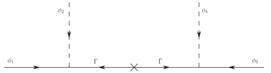
Figure 2: The supergraph for dimension 5 operators in the superpotential of down quarks.

Field	$\phi_{1}$	$\phi_{2}$	$\phi_{3}$	$\phi_{4}$	$\Gamma$
1	$T_{1}$	$H_{\overline{45}}$	$F$	$H_{24}$	$\Upsilon_{1}$
2	$T_{2}$	$H_{24}$	$F$	$H_{\bar{5}}$	$\Upsilon_{2}$
3	$T_{3}$	$H_{\bar{5}}$	$F$	$H_{24}$	$\Upsilon_{3}$

Field	$\Upsilon_{1}$	$\Upsilon_{2}$	$\Upsilon_{3}$
SU(5)	$\overline{\textbf{45}}$	$\overline{\textbf{10}}$	$\bar{\textbf{5}}$
$\Gamma_{4}\equiv S_{4}$	1	$1^{\prime}$	$1^{\prime}$
$k_{I}$	$-1$	3	$-2$

Table 3: Left panel: The dimension 5 operators corresponding to  Figure. 2, Right panel: The charges of messenger fields appear in the dimension 5 operators

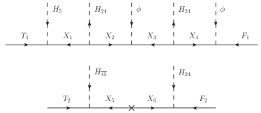
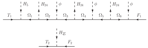
Figure 3: The supergraphs for the operators in Eq. (41) (left) and Eq. (42) (right).

3.3 Neutrino

In this section we shall give the neutrino interactions which induce light neutrino masses. We assume neutrinos to be Majorana type, and the light masses are generated by seesaw mechanism. In most of typical flavor models, including the flavor GUT models, the light neutrino masses can be produced through type-I seesaw mechanism which demands at least two superheavy right-handed Majorana neutrinos to suppress the Yukawa couplings. In the implementation ways of seesaw mechanisms in SU(5) GUTs, however, there are another two ways to do the same thing, the first scheme is type-II seesaw  [57, 58, 59] by adding an extra Higgs $\textbf{15}_{H}$, and the second one is Type-I plus Type-III seesaw [60] by introducing the fermionic fields in the 24 dimensional representation. In our model we assume the second scheme as the unique origin of neutrino masses and no more extra matter fields are involved. The matter chiral superfield $A$ lives in SU(5) adjoint representation 24 and is also an $S_{4}$ triplet. According to the symmetry constraints in , the neutrino Yukawa interactions reads

$$\mathcal{W}_{Y_{A}}=\frac{y_{\nu_{1}}}{\Lambda}FAH_{5}Y_{\bf{3}^{\prime}}+\frac{y_{\nu_{2}}}{\Lambda}F_{3}AH_{5}Y_{\bf{3}^{\prime}}.$$ (43)

Note that the second term would vanish if $(\rho_{F_{3}},\rho_{A})=(\textbf{1},\textbf{3})$ or ($\textbf{1}^{\prime},\textbf{3}^{\prime}$). If we made the choice, the third column of Yukawa texture will be vanishing which features a zero determinant of neutrino mass matrix, no matter what structure of Majorana mass matrix is. We drop the case at present. The Yukawa matrix is then

$$\mathcal{Y}_{\rho_{3}}=\frac{y_{\nu_{1}}}{2}\left[\begin{array}[]{ccc}Y_{4}&Y_{5}&0\\ Y_{3}&Y_{4}&0\\ Y_{5}&Y_{3}&0\\ \end{array}\right]+\frac{y_{\nu_{2}}}{2}\left[\begin{array}[]{ccc}0&0&Y_{3}\\ 0&0&Y_{5}\\ 0&0&Y_{4}\\ \end{array}\right]$$ (50)

$$\mathcal{Y}_{\rho_{0}}=\sqrt{\frac{3}{5}}\mathcal{Y}_{\rho_{3}}.$$ (51)

If we introduce SU(5) singlet 1, e.g., an $N^{c}$, as right-handed Majorana neutrinos, the pure mass term of the form $MN^{c}N^{c}$ is the only interaction. However in adjoint SU(5) there is an extra interaction form besides pure mass term. Since we have 24 dimensional matter superfield responsible for the generation of neutrino masses, the new interactions between 24 and $\textbf{24}_{H}$ have to be considered. Now we give all the mass terms of 24 as

$$\mathcal{W}_{A}=MAAY_{\bf{2}}+M^{\prime}AAY_{\bf{3}^{\prime}}+\lambda_{1}AAH_{24}Y^{(4)}_{\bf{2}}+\lambda_{2}AAH_{24}Y^{(4)}_{\bf{3^{\prime}}}+\lambda_{3}AAH_{24}Y^{(4)}_{\bf{3}}.$$ (52)

The second and the fifth terms vanish because the tensor productions of $\textbf{3}^{\prime}\otimes\textbf{3}^{\prime}$ have to be antisymmetric (see Appendix) to form an invariant with modular forms. Appling the decomposition to eq. (52), the fermionic singlet $\rho_{0}$ and triplet $\rho_{3}$ have the mass matrices of the form

$$M_{\rho_{3}}=$$

$$\frac{M}{4}\left[\begin{array}[]{ccc}0&Y_{1}&Y_{2}\\ Y_{1}&Y_{2}&0\\ Y_{2}&0&Y_{1}\\ \end{array}\right]-\frac{3v^{\prime}_{24}}{4\sqrt{30}}\Big{\{}\lambda_{1}\left[\begin{array}[]{ccc}0&-Y^{2}_{2}&Y^{2}_{1}\\ -Y^{2}_{2}&Y^{2}_{1}&0\\ Y^{2}_{1}&0&-Y^{2}_{2}\\ \end{array}\right]+\lambda_{2}\left[\begin{array}[]{ccc}2Y^{(4)}_{\textbf{3}^{\prime},1}&-Y^{(4)}_{\textbf{3}^{\prime},3}&-Y^{(4)}_{\textbf{3}^{\prime},2}\\ -Y^{(4)}_{\textbf{3}^{\prime},3}&2Y^{(4)}_{\textbf{3}^{\prime},2}&-Y^{(4)}_{\textbf{3}^{\prime},1}\\ -Y^{(4)}_{\textbf{3}^{\prime},2}&-Y^{(4)}_{\textbf{3}^{\prime},1}&2Y^{(4)}_{\textbf{3}^{\prime},3}\\ \end{array}\right]\Big{\}},$$ (62)

$$M_{\rho_{0}}=$$ (63)

$$\frac{M}{4}\left[\begin{array}[]{ccc}0&Y_{1}&Y_{2}\\ Y_{1}&Y_{2}&0\\ Y_{2}&0&Y_{1}\\ \end{array}\right]-\frac{v^{\prime}_{24}}{4\sqrt{30}}\Big{\{}\lambda_{1}\left[\begin{array}[]{ccc}0&-Y^{2}_{2}&Y^{2}_{1}\\ -Y^{2}_{2}&Y^{2}_{1}&0\\ Y^{2}_{1}&0&-Y^{2}_{2}\\ \end{array}\right]+\lambda_{2}\left[\begin{array}[]{ccc}2Y^{(4)}_{\textbf{3}^{\prime},1}&-Y^{(4)}_{\textbf{3}^{\prime},3}&-Y^{(4)}_{\textbf{3}^{\prime},2}\\ -Y^{(4)}_{\textbf{3}^{\prime},3}&2Y^{(4)}_{\textbf{3}^{\prime},2}&-Y^{(4)}_{\textbf{3}^{\prime},1}\\ -Y^{(4)}_{\textbf{3}^{\prime},2}&-Y^{(4)}_{\textbf{3}^{\prime},1}&2Y^{(4)}_{\textbf{3}^{\prime},3}\\ \end{array}\right]\Big{\}},$$ (73)

where the abbreviation $Y^{(4)}_{\textbf{3}^{\prime},i}$($i=1,2,3$) denote the components of weight 4 modular form $Y^{(4)}_{\textbf{3}^{\prime}}$ for the expression more compact, e.g., $Y^{(4)}_{\textbf{3}^{\prime},1}=Y_{1}Y_{4}+Y_{2}Y_{5}$ and else, see Eq. (18).

The neutrino masses are generated by Type-I and Type-III seesaw, which are realized by integrating out $\rho_{0}$ and $\rho_{3}$, respectively. We write the effective light neutrino mass matrix as the sum of the contributions from Type-I and Type-III seesaw

$$M^{SS}_{\nu}=-(\mathcal{Y}^{T}_{\rho_{0}}M^{-1}_{\rho_{0}}\mathcal{Y}_{\rho_{0}}+\mathcal{Y}^{T}_{\rho_{3}}M^{-1}_{\rho_{3}}\mathcal{Y}_{\rho_{3}})v^{2}_{u},$$ (74)

where $v_{u}=v\sin\beta$ with $v=\sqrt{v^{2}_{u}+v^{2}_{d}}=$174GeV and $\tan\beta=v_{u}/v_{d}$, as usual defined in MSSM.

4 Phenomenology

The superpotential in the matter sector is simply given by

$$\mathcal{W}_{\textrm{matt}}=\mathcal{W}_{u}+\mathcal{W}_{d}+\mathcal{W}_{Y_{A}}+\mathcal{W}_{A},$$ (75)

in which each term is given by Eqs. (35), (38),  (43) and (52), respectively. As the GUT and modular symmetry breaking we write the Yukawa matrices of fermions in the following convention

$$W_{Y}=(Y_{u})_{ij}q_{i}\ast H_{u}u^{c}_{j}+(Y_{d})_{ij}q_{i}\ast H_{d}d^{c}_{j}+(Y_{e})_{ij}\ell_{i}\ast H_{d}e^{c}_{j}$$

$$+(\mathcal{Y}_{\rho_{3}})_{ij}\ell^{T}_{i}i\sigma_{2}(\rho_{3})_{j}H_{u}+(\mathcal{Y}_{\rho_{0}})_{ij}\ell^{T}_{i}i\sigma_{2}(\rho_{0})_{j}H_{u}+(M_{\rho_{3}})_{ij}\textrm{Tr}((\rho_{3})_{i}(\rho_{3})_{j})+(M_{\rho_{0}})_{ij}(\rho_{0})_{i}(\rho_{0})_{j},$$ (76)

where $H_{u}$ and $H_{d}$ are the two Higgs doublets in MSSM. The neutrino Yukawa matrices and mass matrices have been given by Eqs. (50) and (3.3) in Sec. 3.3. The Yukawa matrices of charged fermions are then read as

$$Y_{u}=\left[\begin{array}[]{ccc}\alpha_{u}&0&0\\ 0&\beta_{u}Y_{1}Y_{2}&g_{u}\\ 0&-g_{u}&\gamma_{u}\\ \end{array}\right]\equiv\left[\begin{array}[]{ccc}u_{11}&0&0\\ 0&u_{22}&u_{23}\\ 0&-u_{23}&u_{33}\\ \end{array}\right],$$ (77)

for up quarks, and

$$Y_{d}=\left[\begin{array}[]{ccc}\alpha_{d}Y_{2}&-\alpha_{d}Y_{1}&g_{d}\\ \beta_{d}Y_{2}&\beta_{d}Y_{1}&0\\ 0&0&\gamma_{d}\\ \end{array}\right]\equiv\left[\begin{array}[]{ccc}d_{11}&-d_{11}Y_{1}/Y_{2}&d_{13}\\ d_{22}Y_{2}/Y_{1}&d_{22}&0\\ 0&0&d_{33}\\ \end{array}\right],$$ (78)

for down quarks. Observing the Yukawa matrices $Y_{u}$ and $Y_{d}$ are very sparse with some texture zeros, one can conclude the CKM Cabibbo angle $\theta^{q}_{12}$ is totally generated by the mixing in the down sector, and of course the same for the $\theta^{q}_{13}$ as well as CP phase $\delta^{q}$. The mixing in up sector completely determines the angle $\theta^{q}_{23}$.

In SU(5) GUT the Yukawa matrix of charged leptons is the transpose of that of down quarks, i.e., $Y_{e}\sim Y^{T}_{d}$, up to the order one CG coefficients,

$$Y_{e}=\left[\begin{array}[]{ccc}-\frac{1}{2}d_{11}&6d_{22}Y_{2}/Y_{1}&0\\ -\frac{1}{2}d_{11}Y_{1}/Y_{2}&6d_{22}&0\\ -3d_{13}&0&-\frac{3}{2}d_{33}\\ \end{array}\right].$$ (79)

It is obvious that the down quarks and charged leptons follow the following Yukawa ratios

$$\frac{y_{\tau}}{y_{b}}\approx\frac{3}{2},\quad\frac{y_{\mu}}{y_{s}}\approx 6,\quad\frac{y_{e}}{y_{d}}\approx\frac{1}{2},$$ (80)

in which $y_{\ell}$ ($\ell=e,\mu,\tau$) and $y_{d_{i}}$ ($i=d,s,b$) are the eigenvalues of $Y_{e}$ and $Y_{d}$, respectively. Thus the CG factors $C_{1}=1/2$ and $C_{2}=6$ made the double Yukawa ratio $y_{d}y_{\mu}/y_{e}y_{s}=12$ which is in good agreement with the data in Eq. (37).

4.1 SUSY Threshold corrections

The Yukawa couplings and mixing observables are defined at superhigh GUT scale in our model, therefore the values from low energy experiments must run up to the ones at GUT scale. Moreover the SUSY radiative threshold corrections are the requisite factor for matching the MSSM at the SUSY scale $M_{SUSY}$ to the SM [71, 72, 73, 74]. The running of MSSM Yukawa parameters from $M_{Z}$ to $M_{GUT}$ has been analysed in [64], where the $\tan\beta$ enhanced 1-loop SUSY threshold effects are discussed in detail. The matching relations between the eigenvalues of the MSSM and the SM Yukawa coupling matrices are parameterized as

$$y^{\textrm{MSSM}}_{u,c,t}=\frac{y^{\textrm{SM}}_{u,c,t}}{\sin\bar{\beta}},$$ (81)

$$y^{\textrm{MSSM}}_{d,s}=\frac{y^{\textrm{SM}}_{d,s}}{(1+\bar{\eta}_{q})\cos\bar{\beta}},\qquad y^{\textrm{MSSM}}_{b}=\frac{y^{\textrm{SM}}_{b}}{(1+\bar{\eta}_{b})\cos\bar{\beta}},$$ (82)

$$y^{\textrm{MSSM}}_{e,\mu}=\frac{y^{\textrm{SM}}_{e,\mu}}{(1+\bar{\eta}_{\ell})\cos\bar{\beta}},\qquad y^{\textrm{MSSM}}_{\tau}=\frac{y^{\textrm{SM}}_{\tau}}{\cos\bar{\beta}},$$ (83)

and the quark CKM parameters are also corrected by

$$\theta^{q,\textrm{MSSM}}_{i3}=\frac{1+\bar{\eta}_{b}}{1+\bar{\eta}_{q}}\theta^{q,\textrm{SM}}_{i3},\quad\theta^{q,\textrm{MSSM}}_{12}=\theta^{q,\textrm{SM}}_{12},\quad\delta^{q,\textrm{MSSM}}=\delta^{q,\textrm{SM}}.$$ (84)

One can notice, to a good approximation, the threshold corrections have no impact on $\theta^{q}_{12}$ and $\delta^{q}$ and the running of Yukawa couplings $Y^{\textrm{MSSM}}_{f}$ depends only on $\bar{\eta}_{b}$ and $\tan\bar{\beta}$. Especially in the limit that the threshold corrections to charged leptons are neglected, i.e., $\bar{\eta}_{\ell}=0$, then $\tan\bar{\beta}$ reduces to the usual $\tan\beta$. We will adopt the scenario in the model. Nevertheless the $\bar{\eta}_{q}$ can not be dropped. The reason is that the ratio $y_{\mu}/y_{s}$ at GUT scale is approximately 4.5 without SUSY threshold corrections, but the large CG factor 6 in (79) needs a compensation from $\bar{\eta}_{q}$ which is approximately +0.33 [75]. The two CG factors $C_{2}=6$ and $C_{3}=-3/2$ appeared in the Yukawa matrix $Y_{e}$ in Eq. (79) require a relative large $\tan\beta$ to generate substantial threshold corrections. In fact for the large Yukawa coupling ratios in (80), both large $\tan\beta$ and large threshold corrections are required (cf.[76]). Accordingly we set $\tan\beta=35$, $\bar{\eta}_{b}=0.13125$ and $\bar{\eta}_{q}=0.3$. We notice that the threshold parameters can be free, but the fixed values are enough to reproduce correct observables.

4.2 Numerical Analysis

The Yukawa matrices for neutrinos, up- and down- quarks and leptons are presented in Eqs. (74), (77), (78) and (79), respectively. The only common parameter $\tau$ among them has been bounded in the upper half complex plane. Modular symmetry itself, however, is enable to give rise to the hierarchical fermion masses, and mixing parameters. The free parameters appear in the mass matrices are

$$P_{i}=\{\tau,\alpha_{u},\beta_{u},\gamma_{u},g_{u},\alpha_{d},\beta_{d},\gamma_{d},g_{d},y_{\nu_{1}},y_{\nu_{2}},M,\lambda_{1},\lambda_{2},\},$$ (85)

and the physical observables $Q^{\textrm{obs}}$ in the GUT model include

$$Q_{q}=\{y_{u},y_{c},y_{t},y_{d},y_{s},y_{b},\theta^{q}_{12},\theta^{q}_{13},\theta^{q}_{23},\delta^{q}\},$$

$$Q_{\ell}=\{y_{e},y_{\mu},y_{\tau},\Delta\mathcal{M}^{2}_{21},\Delta\mathcal{M}^{2}_{31},\theta^{\ell}_{12},\theta^{\ell}_{13},\theta^{\ell}_{23},\delta^{\ell}\}.$$ (86)

We shall construct a global $\chi^{2}$ function for all the observable quantities when fitting the coupling matrices in Eqs.(77), (78) and (79) for charged fermions and Eqs. (50) and (3.3) for neutrinos. The $\chi^{2}$ function to be minimized is defined as

$$\chi^{2}=\sum_{i}\Big{(}\frac{Q_{i}(P_{j})-Q^{\textrm{obs}}_{i}}{\sigma_{i}}\Big{)}^{2},$$ (87)

where $Q_{i}(P_{j})$ denote the model predicted values for observables and $Q^{\textrm{obs}}=Q_{q}+Q_{\ell}$ are the central values with $\sigma_{i}$ the $1\sigma$ errors.

Before performing the fit, we would like to elucidate the data used in the minimization. As stressed in Sec. 4.1, the model is defined at the high energy scale, the observable quantities should be set at the GUT scale. The quantities at GUT energy scale can be achieved from the low energy scale where the experimental values are determined by the renormalization group equations (RGEs). Here in our work we adopt the values of Yukawa couplings at the GUT scale $M_{X}=2\times 10^{16}$GeV, assuming minimal SUSY breaking $M_{SUSY}=$1TeV with a large $\tan\beta=35$ [64]. The Yukawa values $y_{f}$ give rise to the fermion masses as $m_{f}=y_{f}v_{H}$ with $v_{H}$=174GeV. Meanwhile the CKM mixing angles and CP phase are also taken as the values at the GUT scale. All the Yukawa values and CKM observables as well as their $1\sigma$ errors are listed in the left panel of Table 4. For the neutrino sector, the lepton mixing angles, CP phase and neutrino mass squared differences we adopted are taken from NuFit 5.0 [77]. We show their center values and $1\sigma$ errors in the right panel of Table 4. The above input data are used for the estimation of our $\chi^{2}$.

Since the quark sector and neutrino sector have the modulus $\tau$ as the common parameter which determines the modular forms, the remaining free parameters are just Yukawa coupling coefficients. It is equivalent and more convenient to fit the entries of Yukawa matrices rather than Yukawa coefficients themselves. Therefore we just fit the entries of quark Yukawa matrices, $u_{ij}$s in Eq. (77) and $d_{ij}$s in Eq. (78). In neutrino sector, we define the coupling parameter ratios

$$r_{21}=\frac{y_{\nu_{2}}}{y_{\nu_{1}}},\qquad r_{1}=\frac{\lambda_{1}v_{24}}{M},\qquad r_{2}=\frac{\lambda_{2}v_{24}}{M},$$ (88)

and an overall mass scale $y^{2}_{\nu_{1}}v^{2}_{u}/M$ are the parameters to be fitted. So, instead of fitting the primitive free parameters showed in Eq. (85), we take the following equivalent parameter set

$$\overline{P}_{i}=\{\tau,u_{11},u_{22},u_{33},u_{23},d_{11},d_{22},d_{33},d_{13},r_{21},r_{1},r_{2},y^{2}_{\nu_{1}}v^{2}_{u}/M\}.$$ (89)

In Table 5 we show the model best fit input parameters in quark Yukawa and neutrino mass matrices which minimizes the $\chi^{2}_{q}$ and $\chi^{2}_{\ell}$, respectively. We present our fit results for all the Yukawas and mass matrices in Table 6. In the left panel of Table 6 we give the resulting best fit values and pulls to the ten quark observables: three quark CKM mixing angles $\theta^{q}_{ij}$ ($ij=12,13,23$) and one CP violating phase $\delta^{q}$, six Yukawas $y_{q}$ ($q=u,c,t,d,s,b$). Also the minimum $\chi^{2}_{\textrm{min},q}\sim 0.45$ is given at the last row. We also list in Table 6 (right panel) the best fit values and pulls to six neutrino observables and three charged lepton Yukawas. The minimum $\chi^{2}_{\textrm{min},\ell}$ is just $\mathcal{O}(1)$. The best fit point has the total $\chi^{2}_{\textrm{min}}=\chi^{2}_{\textrm{min},q}+\chi^{2}_{\textrm{min},\ell}\simeq 1.6$. One can see that the model favours normal ordering neutrino masses, and we found the minimum $\chi^{2}_{\textrm{min},\ell}=8.478$ for inverted ordering. Besides the values of absolute neutrino masses $m_{i}$, the Majorana phases $\varphi_{21}$ and $\varphi_{31}$ are pure theoretical predictions. The mass sum, the $\beta$-decay effective mass $m_{\beta}$ as well as the neutrinoless double beta ($0\nu\beta\beta$) decay amplitude parameter $m_{ee}$ are also given as predictions in the table. Specifically the bounds on the above mass related quantities are given by

$$\sum_{i}m_{i}\leq 120\textrm{meV},$$

$$m_{\beta}=\Big{[}\sum_{i}m^{2}_{i}|U_{ei}|^{2}\Big{]}^{1/2}<(61\sim 165)\textrm{meV},$$ (90)

$$m_{ee}=\Big{|}\sum_{i}U^{2}_{ei}m_{i}\Big{|}<1.1\textrm{eV}(90\%\textrm{C.L.}),$$

which are taken from PLANCK[78], KamLAND-ZEN [79] and KATRIN [80], respectively. The leptonic mixing matrix elements $U_{ei}$ are taken from the standard parametrization [3]

$$U=\left(\begin{array}[]{ccc}c_{12}c_{13}&s_{12}c_{13}&s_{13}e^{-i\delta}\\ -s_{12}c_{23}-c_{12}s_{13}s_{23}e^{i\delta}&c_{12}c_{23}-s_{12}s_{13}s_{23}e^{i\delta}&c_{13}s_{23}\\ s_{12}s_{23}-c_{12}s_{13}c_{23}e^{i\delta}&-c_{12}c_{23}-s_{12}s_{13}c_{23}e^{i\delta}&c_{13}c_{23}\\ \end{array}\right)\left(\begin{array}[]{ccc}1&0&0\\ 0&e^{\varphi_{21}/2}&0\\ 0&0&e^{\varphi_{31}/2}\\ \end{array}\right),$$ (91)

where $s_{ij}=\sin\theta_{ij}$, $c_{ij}=\cos\theta_{ij}$, $\delta$ is lepton Dirac CP violating phase and $\varphi_{21}$, $\varphi_{31}$ are two Majorana CP phases. Comparing the model predictions in Table 6 to these bounds, we see that the predicted values are well below the corresponding upper bounds. For the sum of neutrino masses, our result is still below the tightest and most rebust upper limit $M_{\nu}<0.118$eV [81].

There are 17 real input parameters in Table 5, to fit 19 measured data points in Table 4. Hence the number of the degree of freedom (d.o.f) is naively 2, which is the difference of the number of observables and inputs. This translates to a reduced $\chi^{2}$, i.e., $\chi^{2}_{\textrm{red}}=\chi^{2}_{\textrm{min}}/\textrm{d.o.f}=0.808$. We take this value as a good fit. The fit has been performed by using the Mathematica package Mixing Parameter Tools (MPT) [82].

We can see that in quark and lepton sectors the only common input parameter is modulus $\tau$, which is close to the boundary (right cusp) of the fundamental region. The Yukawas are in general complex, however we can always absorb most of the phases by redefinition of the fields. Specifically for the quark Yukawa inputs, the only complex parameter is $d_{13}$ which mainly controls the magnitude of the CKM matrix element $V_{ub}$ and part of the CP phase $\delta^{q}$. Meanwhile the other inputs, all $u_{ij}$s and the rest of $d_{ij}$s ($ij\neq 13$) are real. In neutrino sector we also have reduced the total number of real parameters to be six, in which only $r_{1}$ and $r_{2}$ are complex. The Yukawa ratio $r_{21}$ and the overall mass scale $y^{2}_{\nu_{1}}v^{2}_{u}/M$ are all real parameters.

Observable	$\mu_{i}$	$\sigma_{i}$
$\theta^{q}_{12}/^{\circ}$	13.027	0.041
$\theta^{q}_{13}/^{\circ}$	0.166	0.006
$\theta^{q}_{23}/^{\circ}$	1.924	0.031
$\delta^{q}/^{\circ}$	69.213	3.094
$y_{u}$	$2.889\times 10^{-6}$	$8.954\times 10^{-7}$
$y_{c}$	$1.413\times 10^{-3}$	$4.946\times 10^{-5}$
$y_{t}$	0.529	0.016
$y_{d}$	$1.3879\times 10^{-4}$	$1.5267\times 10^{-5}$
$y_{s}$	$2.7467\times 10^{-3}$	$1.4832\times 10^{-4}$
$y_{b}$	0.1867	$2.766\times 10^{-3}$
$y_{e}$	$7.3834\times 10^{-5}$	$4.430\times 10^{-7}$
$y_{\mu}$	$1.5590\times 10^{-2}$	$9.354\times 10^{-5}$
$y_{\tau}$	0.2819	$1.751\times 10^{-3}$

Observable	NO	IO
$\theta_{12}/^{\circ}$	$33.44^{+0.78}_{-0.75}$	$33.45^{+0.78}_{-0.75}$
$\theta_{13}/^{\circ}$	$8.57^{+0.13}_{-0.12}$	$8.61\pm 0.12$
$\theta_{23}/^{\circ}$	$49.0^{+1.0}_{-1.4}$	$49.3^{+1.0}_{-1.2}$
$\delta/^{\circ}$	$195^{+51}_{-25}$	$286^{+27}_{-32}$
$\Delta\mathcal{M}^{2}_{21}/10^{-5}$	$7.42^{+0.21}_{-0.20}$	$7.42^{+0.21}_{-0.20}$
$\Delta\mathcal{M}^{2}_{31}/10^{-3}$	$2.514^{+0.028}_{-0.027}$	$-2.497^{+0.028}_{-0.028}$

Table 4: Left panel: The Observables of charged fermions at the GUT scale for $\tan\beta=35$ are taken from [64]. The SUSY breaking scale are set at $M_{SUSY}=$1TeV and the threshold correction parameters $\bar{\eta}_{b}=0.13125$ and $\bar{\eta}_{q}=0.3$. Right panel: The values of neutrino Observables are taken from NuFit5.0  [77] without the atmospheric data from SuperKamiokande. NO (IO) denotes the Normal (Inverted) Ordering of neutrino masses.

Quark Input	Value
$u_{11}$	$2.887\times 10^{-6}$
$u_{22}$	$8.476\times 10^{-4}$
$u_{33}$	$0.5304$
$u_{23}$	$-1.775\times 10^{-2}$
$d_{11}$	$2.667\times 10^{-6}$
$d_{22}$	$1.020\times 10^{-4}$
$d_{33}$	$6.032\times 10^{-3}$
$d_{13}$	$2.031\times 10^{-5}\textrm{e}^{-0.657i\pi}$

Neutrino Input	Value
$r_{1}=\lambda_{1}v_{24}/M$	$-0.06587+2.09536i$
$r_{2}=\lambda_{2}v_{24}/M$	$0.36449+1.72602i$
$r_{21}=y_{\nu_{2}}/y_{\nu_{1}}$	2.26385
$y_{\nu_{1}}^{2}v^{2}_{u}/M(\textrm{eV})$	0.00362

Common Input	Value
$\texttt{Re}\tau$	$0.4768$
$\texttt{Im}\tau$	$0.9288$

Table 5: Left panel: The best fit input parameters in quark sector. The Yukawa entries $u_{ij}$ and $d_{ij}$ include the original Yukawa coupling coefficients and the modular forms. Upper Right panel: The best fit input parameters in neutrino sector. We list the ratios of neutrino couplings in eqs. (43) and (52). Lower Right panel: The only common input parameter to both sectors is the modulus $\tau$.

Quark output	Value		pull
$\theta^{q}_{12}/^{\circ}$	13.0233		$-0.0839$
$\theta^{q}_{13}/^{\circ}$	0.16639		0.0002
$\theta^{q}_{23}/^{\circ}$	1.9238		0
$\delta^{q}/^{\circ}$	69.0969		0.0376
$y_{u}$	$2.889\times 10^{-6}$		0.0
$y_{c}$	$1.413\times 10^{-3}$		0.0
$y_{t}$	0.529		0.0
$y_{d}$	$1.4378\times 10^{-4}$		0.327
$y_{s}$	$2.6685\times 10^{-3}$		$-0.527$
$y_{b}$	0.1873		0.2312
$\chi^{2}_{\textrm{min},q}$			0.4467

Lepton output	Value		pull
$\theta_{12}/^{\circ}$	33.4916		0.0675
$\theta_{13}/^{\circ}$	8.5344		$-0.285$
$\theta_{23}/^{\circ}$	49.7665		0.613
$\delta/^{\circ}$	208.2733		0.349
$\Delta\mathcal{M}^{2}_{21}/10^{-5}$	7.524		0.4966
$\Delta\mathcal{M}^{2}_{31}/10^{-3}$	2.514		0
$y_{e}$	$7.377\times 10^{-5}$		$-0.1432$
$y_{\mu}$	$1.560\times 10^{-2}$		0.1433
$y_{\tau}$	0.281		$-0.5478$
$\chi^{2}_{\textrm{min},\ell}$			1.1694
Predictions	Value
Mass Ordering	NO
$m_{1}/\textrm{meV}$	11.728
$m_{2}/\textrm{meV}$	14.585
$m_{3}/\textrm{meV}$	51.493
$\sum_{i}m_{i}/\textrm{meV}$	77.809
$m_{\beta}/\textrm{meV}$	14.674
$m_{ee}/\textrm{meV}$	11.040
$\varphi_{21}/\pi$	0.105
$\varphi_{31}/\pi$	1.323

Table 6: Left panel: The quark fit output results. All the quark sector is fitted to the $1\sigma$ interval. Right panel: The output results of lepton sector. The absolute values of three light neutrino masses and the ordering as well as the two Majorana phases are pure model predictions. We have found a minimum $\chi^{2}_{\textrm{min},\ell}=8.478$ for inverted ordering.

5 Summary

In the study we explored an supersymmetric adjoint SU(5) GUT flavor model based on modular $\Gamma_{4}\simeq S_{4}$ symmetry. We have shown the model can produce correct masses and mixing parameters of both quarks and leptons simultaneously. No flavons are introduced to the model, only the complex modulus $\tau$ is responsible for the breaking of modular symmetry. By assigning suitable representations and weights to chiral superfields, only finite coupling terms are presented in the effective operators in quark sector and lepton sector. We obtained very sparse Yukawa matrices of up- and down-quarks (and of course charged leptons) with some texture zeros. Also in neutrino sector we have only two Yukawa coupling terms, and three terms in Majorana mass terms. The effective light neutrino masses are generated through Type-I plus Type-III seesaw mechanism. The modulus $\tau$ is the only common field appeared in both quark and lepton sector as spurion.

For simplicity we have used modular forms with lower weight in the model, since higher weight would bring more free parameters. The assignments of representations under $S_{4}$ and weights for the chiral superfields are also highly constrained such that the Yukawa coupling terms are uniquely fixed by the modular forms. The 10 dimensional matter fields are all $S_{4}$ singlets, while $\bar{\textbf{5}}$s are divided into a $S_{4}$ doublet for the first two generations and a singlet for third one. Meanwhile the adjoint superfields 24 are collected in the triplet of $S_{4}$. All the scalars of course transform as singlets of $S_{4}$. We also assigned distinct weights for the superfields such that the number of free Yukawa parameters is as little as possible.

With the delicate representation assignments of field content, the superpotentials of the model is relatively simple. Unlike the models in  [32, 21] which have more parameters than observables, our model has less free parameters and thus more predictive than the above two works. The resulting operators in each sector have limit coupling parameters. The model predicts that down quarks and charged leptons have a rigid Yukawa coupling ratios generated by CG factors which arise from the SU(5) contractions of the effective 5D operators. The double Yukawa ratio $y_{\mu}y_{d}/y_{e}y_{s}$ equal to 12 for the first two families of charged leptons and down quarks. The model has only 17 real parameters in total, and 19 observables to be fit, thus the degree of freedom (d.o.f) is 2. We obtained the reduced chi-square $\chi^{2}/\textrm{d.o.f}\simeq 0.81$ for quark and lepton sectors combined, which is a good fit. The model favours an normal mass ordering over inverted ordering for light neutrinos, with a $\Delta\chi^{2}\sim 7$. Moreover we obtained the absolute values of three light neutrino masses, the effective masses of $\beta$-decay and $0\nu\beta\beta$ decay as well as the Majorana CP phases as model predictions.

At last we give a outlook for the model. Since the masses of the fields live in the adjoint representation are splited by the adjoint scalar $H_{24}$, the lightest one is $\rho_{3}$. It is crucial to realize the baryogenesis via leptogenesis  [83, 84] in the context. In the case the net asymmetry of $B-L$ can be generated in the out of equilibrium decays of $\rho_{3}$ and $\rho_{0}$ as well as their superpartners in the adjoint representation. So it is worth studying further the phenomenology according to the model.

APPENDIX: $S_{4}$ GROUP

The discrete group $S_{4}$ who has 24 elements is the permutation group of four objects. The two generators S and T in different irreducible presentations are given as follows

$$\textbf{1}:S=1,\quad T=1$$ (A1)

$$\textbf{1}^{\prime}:S=-1,\quad T=1$$ (A2)

$$\textbf{2}:S=\left(\begin{array}[]{cc}0&1\\ 1&0\\ \end{array}\right),\quad T=\left(\begin{array}[]{cc}\omega&0\\ 0&\omega^{2}\\ \end{array}\right)$$ (A7)

$$\textbf{3}:S=\frac{1}{3}\left(\begin{array}[]{ccc}-1&2\omega&2\omega^{2}\\ 2\omega&2\omega^{2}&-1\\ 2\omega^{2}&-1&2\omega\\ \end{array}\right),\quad T=\left(\begin{array}[]{ccc}1&0&0\\ 0&\omega^{2}&0\\ 0&0&\omega\\ \end{array}\right)$$ (A14)

$$\textbf{3}^{\prime}:S=\frac{1}{3}\left(\begin{array}[]{ccc}1&-2\omega&-2\omega^{2}\\ -2\omega&-2\omega^{2}&1\\ -2\omega^{2}&1&-2\omega\\ \end{array}\right),\quad T=\left(\begin{array}[]{ccc}1&0&0\\ 0&\omega^{2}&0\\ 0&0&\omega\\ \end{array}\right)$$ (A21)

where $\omega=e^{2\pi i/3}=(i\sqrt{3}-1)/2$. In the basis we can obtain the decomposition of the product representations and the Clebsch-Gordan factors. The product rules of $S_{4}$ group, with $a_{i}$, $b_{i}$ as the elements of multiplet in the product, are given by following

$$\star\quad\bf{1}\otimes r=r\sim\emph{ab}_{\emph{i}}$$ (A22)

$$\star\quad\bf{1}^{\prime}\otimes 1^{\prime}=1\sim\emph{ab}$$ (A23)

$$\star\quad\bf{1}^{\prime}\otimes 2=2\sim\left(\begin{array}[]{c}ab_{1}\\ -ab_{2}\\ \end{array}\right)$$ (A26)

$$\star\quad\bf{1}^{\prime}\otimes 3=3^{\prime}\sim\left(\begin{array}[]{c}ab_{1}\\ ab_{2}\\ ab_{3}\\ \end{array}\right)$$ (A30)

$$\star\quad\bf{1}^{\prime}\otimes 3^{\prime}=3\sim\left(\begin{array}[]{c}ab_{1}\\ ab_{2}\\ ab_{3}\\ \end{array}\right)$$ (A34)

The product rules with two-dimensional representation are given by:

$$\star\quad\bf{2}\otimes 2=1\oplus 1^{\prime}\oplus 2$$

$$\quad\quad\textbf{1}\sim a_{1}b_{2}+a_{2}b_{1},\quad\quad\textbf{1}^{\prime}\sim a_{1}b_{2}-a_{2}b_{1}$$

$$\quad\quad\textbf{2}\sim\left(\begin{array}[]{c}a_{2}b_{2}\\ a_{1}b_{1}\\ \end{array}\right)$$ (A37)

$$\star\quad\bf{2}\otimes 3=3\oplus 3^{\prime}$$

$$\quad\quad\textbf{3}\sim\left(\begin{array}[]{c}a_{1}b_{2}+a_{2}b_{3}\\ a_{1}b_{3}+a_{2}b_{1}\\ a_{1}b_{1}+a_{2}b_{2}\\ \end{array}\right),\quad\quad\textbf{3}^{\prime}\sim\left(\begin{array}[]{c}a_{1}b_{2}-a_{2}b_{3}\\ a_{1}b_{3}-a_{2}b_{1}\\ a_{1}b_{1}-a_{2}b_{2}\\ \end{array}\right)$$ (A44)

$$\star\quad\bf{2}\otimes 3^{\prime}=3\oplus 3^{\prime}$$

$$\quad\quad\textbf{3}\sim\left(\begin{array}[]{c}a_{1}b_{2}-a_{2}b_{3}\\ a_{1}b_{3}-a_{2}b_{1}\\ a_{1}b_{1}-a_{2}b_{2}\\ \end{array}\right),\quad\quad\textbf{3}^{\prime}\sim\left(\begin{array}[]{c}a_{1}b_{2}+a_{2}b_{3}\\ a_{1}b_{3}+a_{2}b_{1}\\ a_{1}b_{1}+a_{2}b_{2}\\ \end{array}\right)$$ (A51)

and the three-dimensional representations have the following product rules

$$\star\quad\bf{3}\otimes 3=3^{\prime}\otimes 3^{\prime}=1\oplus 2\oplus 3\oplus 3^{\prime}$$

$$\quad\quad\textbf{1}\sim a_{1}b_{1}+a_{2}b_{3}+a_{3}b_{2}$$

$$\quad\quad\textbf{2}\sim\left(\begin{array}[]{c}a_{2}b_{2}+a_{3}b_{1}+a_{1}b_{3}\\ a_{3}b_{3}+a_{1}b_{2}+a_{2}b_{1}\\ \end{array}\right)$$ (A54)

$$\quad\quad\textbf{3}\sim\left(\begin{array}[]{c}2a_{1}b_{1}-a_{2}b_{3}-a_{3}b_{2}\\ 2a_{3}b_{3}-a_{1}b_{2}-a_{2}b_{1}\\ 2a_{2}b_{2}-a_{3}b_{1}-a_{1}b_{3}\\ \end{array}\right),\quad\quad\textbf{3}^{\prime}\sim\left(\begin{array}[]{c}a_{2}b_{3}-a_{3}b_{2}\\ a_{1}b_{2}-a_{2}b_{1}\\ a_{3}b_{1}-a_{1}b_{3}\\ \end{array}\right)$$ (A61)

$$\star\quad\bf{3}\otimes 3^{\prime}=1^{\prime}\oplus 2\oplus 3\oplus 3^{\prime}$$

$$\quad\quad\textbf{1}^{\prime}\sim a_{1}b_{1}+a_{2}b_{3}+a_{3}b_{2}$$

$$\quad\quad\textbf{2}\sim\left(\begin{array}[]{c}a_{2}b_{2}+a_{3}b_{1}+a_{1}b_{3}\\ -a_{3}b_{3}-a_{1}b_{2}-a_{2}b_{1}\\ \end{array}\right)$$ (A64)

$$\quad\quad\textbf{3}\sim\left(\begin{array}[]{c}a_{2}b_{3}-a_{3}b_{2}\\ a_{1}b_{2}-a_{2}b_{1}\\ a_{3}b_{1}-a_{1}b_{3}\\ \end{array}\right),\quad\quad\textbf{3}^{\prime}\sim\left(\begin{array}[]{c}2a_{1}b_{1}-a_{2}b_{3}-a_{3}b_{2}\\ 2a_{3}b_{3}-a_{1}b_{2}-a_{2}b_{1}\\ 2a_{2}b_{2}-a_{3}b_{1}-a_{1}b_{3}\\ \end{array}\right)$$ (A71)

References

- [1] ATLAS Collaboration, G. Aad et al., “Observation of a new particle in the search for the Standard Model Higgs boson with the ATLAS detector at the LHC”, Phys. Lett. B 716 (2012) 1, [arXiv:1207.7214 [hep-ex]].
- [2] CMS Collaboration, S. Chatrchyan et al., “Observation of a new boson at a mass of 125 GeV with the CMS experiment at the LHC”, Phys. Lett. B 716 (2012) 30, [arXiv:1207.7235 [hep-ex]].
- [3] Particle Data Group Collaboration, M. Tanabashi et al., “Review of Particle Physics”, Phys. Rev. D 98 (2018) 030001.
- [4] L.J. Hall, H. Murayama and N. Weiner, “Neutrino Mass Anarchy”, Phys. Rev. Lett. 84 (2000) 2572, [arXiv:hep-ph/9911341].
- [5] K.R. Dienes, E. Dudas and T. Gherghetta, “Light neutrinos without heavy mass scales: a higher-dimensional seesaw mechanism”, Nucl. Phys. B 557 (1999) 25, [arXiv:hep-ph/9811428].
- [6] N. Arkani-Hamed, S. Dimopoulos, G.R. Dvali and J. March-Russell, “Neutrino masses from large extra dimensions”, Phys. Rev. D 65 (2002) 024032, [arXiv:hep-ph/9811448].
- [7] R. Blumenhagen, M. Cvetič and T. Weigand, “Spacetime instanton corrections in 4D string vacua: The seesaw mechanism for D-brane models”, Nucl. Phys. B 771 (2007) 113, [arXiv:hep-th/0609191].
- [8] L.E. Ibáñez and A.M. Uranga, “Neutrino Majorana masses from string theory instanton effects”, JHEP 03 (2007) 052, [arXiv:hep-th/0609213].
- [9] S. Antusch, L.E. Ibáñez and T. Macrì, “Neutrino masses and mixings from string theory instantons”, JHEP 09 (2007) 087, [arXiv:0706.2132 [hep-ph]].
- [10] G. Altarelli and F. Feruglio, “Discrete flavor symmetries and models of neutrino mixing”, Rev. Mod. Phys. 82 (2010) 2701, [arXiv:1002.0211 [hep-ph]].
- [11] H. Ishimori, T. Kobayashi, H. Ohki, Y. Shimizu, H. Okada and M. Tanimoto, “Non-Abelian Discrete Symmetries in Particle Physics”, Prog. Theor. Phys. Suppl. 183 (2010) 1-163, [arXiv:1003.3552 [hep-th]].
- [12] S.F. King and C. Luhn, “Neutrino mass and mixing with discrete symmetry”, Rep. Prog. Phys. 76 (2013) 056201, [arXiv:1301.1340 [hep-ph]].
- [13] S.F. King, “Models of neutrino mass, mixing and CP violation”, J. Phys. G 42 (2015) 123001, [arXiv:1510.02091 [hep-ph]].
- [14] S.F. King, “Unified models of neutrinos, flavour and CP Violation”, Prog. Part. Nucl.Phys. 94 (2017) 217, [arXiv:1701.04413 [hep-ph]].
- [15] D. Meloni, “GUT and Flavor Models for Neutrino Masses and Mixing”, Frontiers in Physics 5 (2017) 43, [arXiv:1709.02662 [hep-ph]].
- [16] P.F. Harrison, D.H. Perkins and W.G. Scott, “Tri-bimaximal mixing and the neutrino oscillation data”, Phys. Lett. B 530 (2002) 167, [arXiv:hep-ph/0202074].
- [17] P.F. Harrison and W.G. Scott, Phys. Lett. B 535 (2002) 163, [arXiv:hep-ph/0203209].
- [18] F. Feruglio, “Are neutrino masses modular forms?”, in book “From my vast repertoire:the legacy of Guido Altarelli”, S. Forte, A.Levy and G. Ridolfi, eds, [arXiv:1706.08749 [hep-ph]].
- [19] T. Kobayashi, K. Tanaka, and T. H. Tatsuishi, “Neutrino mixing from finite modular groups”, Phys. Rev. D 98 (2018) 016004, [arXiv:1803.10391 [hep-ph]].
- [20] H. Okada and Y. Orikasa, “Modular symmetric radiative seesaw model”, Phys. Rev. D 100 (2019) 115037, [arXiv:1907.04716 [hep-ph]].
- [21] T. Kobayashi, Y. Shimizu, K. Takagi, M. Tanimoto and Takuya H. Tatsuishi, “Modular -invariant flavor model in SU(5) grand unified theory”, Prog. Theor. Exp. Phys. 053B (2020) 05, [arXiv:1906.10341 [hep-ph]].
- [22] S. Mishra, “Neutrino mixing and Leptogenesis with modular symmetry in the framework of type III seesaw”, [arXiv:2008.02095 [hep-ph]].
- [23] J.C. Criado and F. Feruglio, “Modular Invariance Faces Precision Neutrino Data”, SciPost Phys. 5 (2018) 042, [arXiv:1807.01125 [hep-ph]].
- [24] H. Okada and M. Tanimoto, “CP violation of quarks in modular invariance”, [arXiv:1812.09677 [hep-ph]].
- [25] H. Okada and M. Tanimoto, “Quark and lepton flavors with common modulus in modular symmetry”, [arXiv:2005.00775 [hep-ph]].
- [26] T. Kobayashi, Y. Shimizu, K. Takagi, M. Tanimoto, T. H. Tatsuishi and H. Uchida, “Finite modular subgroups for fermion mass matrices and baryon/lepton number violation”, Phys. Lett. B 794 (2019) 114, [arXiv:1812.11072 [hep-ph]].
- [27] T. Nomura and H. Okada, “A modular symmetric model of dark matter and neutrino”, Phys. Lett. B 797 (2019) 134799, [arXiv:1904.03937 [hep-ph]].
- [28] T. Nomura, and H. Okada, “A two loop induced neutrino mass model with modular symmetry”, [arXiv:1906.03927 [hep-ph]].
- [29] G.-J. Ding, and S. F. King, and X.-G. Liu, “Modular symmetry models of neutrinos and charged leptons”, JHEP 09 (2019) 074, [arXiv:1907.11714 [hep-ph]].
- [30] T. Kobayashi, Y. Shimizu, K. Takagi, M. Tanimoto and Takuya H. Tatsuishi, “New lepton flavor model from modular symmetry”, JHEP 02 (2020) 097, [arXiv:1907.09141 [hep-ph]].
- [31] Simon J. D. King, S. F. King, “Fermion Mass Hierarchies from Modular Symmetry”, JHEP 09 (2020) 043, [arXiv:2002.00969 [hep-ph]].
- [32] F.J. de Anda, and S. F. King, and E. Perdomo, “ grand unified theory with modular symmetry”, Phys. Rev. D 101 (2020) 015028, [arXiv:1812.05620 [hep-ph]].
- [33] T. Asaka, Y. Heo, T. H. Tatsuishi and T. Yoshida, “Modular invariance and leptogenesis”, JHEP 01 (2020) 144, [arXiv:1909.06520 [hep-ph]].
- [34] M.K. Behera, S. Mishra, S. Singirala and R. Mohanta, “Implications of modular symmetry on Neutrino mass, Mixing and Leptogenesis with Linear Seesaw”, [arXiv:2007.00545 [hep-ph]].
- [35] J. Penedo and S. Petcov, “Lepton Masses and Mixing from Modular Symmetry”, Nucl. Phys. B 939 (2019) 292, [arXiv:1806.11040 [hep-ph]].
- [36] P. Novichkov, J. Penedo, S. Petcov, and A. Titov, “Modular S4 models of lepton masses and mixing”, JHEP 04 (2019) 005, [arXiv:1811.04933 [hep-ph]].
- [37] I. de Medeiros Varzielas, S. F. King, and Y.-L. Zhou, “Multiple modular symmetries as the origin of flavor”, Phys. Rev. D 101 (2020) 055033, [arXiv:1906.02208 [hep-ph]].
- [38] G.-J. Ding, S. F. King, X.-G. Liu, and J.-N. Lu, “Modular S4 and A4 symmetries and their fixed points: new predictive examples of lepton mixing”, JHEP 12 (2019) 030, [arXiv:1910.03460 [hep-ph]].
- [39] T. Kobayashi, Y. Shimizu, K. Takagi, M. Tanimoto, and T. H. Tatsuishi, “New lepton flavor model from modular symmetry”, JHEP 02 (2020) 097, [arXiv:1907.09141 [hep-ph]].
- [40] S. F. King and Y.-L. Zhou, “Trimaximal TM1 mixing with two modular groups”, Phys. Rev. D 101 (2020) 015001, [arXiv:1908.02770 [hep-ph]].
- [41] J. C. Criado, F. Feruglio, and S. J. King, “Modular Invariant Models of Lepton Masses at Levels 4 and 5”, JHEP 02 (2020) 001, [arXiv:1908.11867 [hep-ph]].
- [42] X. Wang and S. Zhou, “The minimal seesaw model with a modular S4 symmetry”, JHEP 05 (2020) 017, [arXiv:1910.09473 [hep-ph]].
- [43] X. Wang, “A systematic study of Dirac neutrino mass models with a modular symmetry”, [arXiv:2007.05913 [hep-ph]].
- [44] P. Novichkov, J. Penedo, S. Petcov, and A. Titov, “Modular A5 symmetry for flavour model building”, JHEP 04 (2019) 174, [arXiv:1812.02158 [hep-ph]].
- [45] G.-J. Ding, S. F. King, and X.-G. Liu, “Neutrino mass and mixing with modular symmetry” Phys. Rev. D 100 (2019) 115005, [arXiv:1903.12588 [hep-ph]].
- [46] X.-G. Liu and G.-J. Ding, “Neutrino Masses and Mixing from Double Covering of Finite Modular Groups”, [arXiv:1907.01488 [hep-ph]].
- [47] J.-N. Lu, X.-G. Liu, and G.-J. Ding, “Modular symmetry origin of texture zeros and quark lepton unification”, Phys. Rev. D 101 (2020) 115020, [arXiv:1912.07573 [hep-ph]].
- [48] P. P. Novichkov, J. T. Penedo, S. T. Petcov, “Double Cover of Modular for Flavour Model Building”, [arXiv:2006.03058 [hep-ph]].
- [49] X.-G. Liu, C.-Y. Yao, G.-J. Ding, “Modular Invariant Quark and Lepton Models in Double Covering of Modular Group,”, [arXiv:2006.10722 [hep-ph]].
- [50] X. Wang, B. Yu, and S. Zhou, “Double Covering of the Modular Group and Lepton Flavor Mixing in the Minimal Seesaw Model”, [arXiv:2010.10159 [hep-ph]].
- [51] C.-Y. Yao, X.-G. Liu, G.-J. Ding “Fermion Masses and Mixing from Double Cover and Metaplectic Cover of Modular Group”, [arXiv:2011.03501 [hep-ph]].
- [52] P. Fileviez Pérez, “Supersymmetric adjoint SU(5)”, Phys. Rev. D 76 (2007) 071701, [arXiv:0705.3589 [hep-ph]].
- [53] P. Minkowski, “ at a rate of one out of muon decays?”, Phys. Lett. B 67 (1977) 421.
- [54] T. Yanagida, 1979, “Horizontal symmetry and masses of neutrinos”, in the proceedings of the “Workshop on Unified Theory and Baryon Number in the Universe”, O. Sawada and A. Sugamoto eds., KEK, Tsukuba, Japan (1979).
- [55] R.N. Mohapatra and G. Senjanović, “Neutrino Mass and Spontaneous Parity Nonconservation”, Phys. Rev. Lett. 44 (1980) 912.
- [56] M. Gell-Mann, P. Ramond and R. Slansky, “Complex Spinors and Unified Theories”, In “Supergravity”, D.Z. Freedman and F. van Nieuwenhuizen eds., North Holland, Amsterdam, The Netherlands (1979), [arXiv:1306.4669 [hep-th]].
- [57] G. Lazarides and Q. Shafi and C. Wetterich, “Proton lifetime and fermion masses in an SO(10) model”, Nucl. Phys. B 181 (1981) 287.
- [58] J. Schechter and J.W.F. Valle, “Neutrino masses in SU(2)U(1) theories”, Phys. Rev. D 22 (1980) 2227.
- [59] R.N. Mohapatra and S. Goran, “Neutrino masses and mixings in gauge models with spontaneous parity violation”, Phys. Rev. D 23 (1981) 165.
- [60] R. Foot, H. Lew, X.-G. He and G.C. Joshi, “See-saw neutrino masses induced by a triplet of leptons”, Z. Phys. C 44 (1989) 441.
- [61] P. Fileviez Pérez, “Renormalizable adjoint SU(5)”, Phys. Lett. B 654 (2007) 189, [arXiv:hep-ph/0702287].
- [62] D. Binosi and L. Theußl, “JaxoDraw: A graphical user interface for drawing Feynman diagrams”, Comput. Phys. Commun. 161 (2004) 76, [arXiv:hep-ph/0309015].
- [63] D. Binosi, J. Collins, C. Kaufhold and L. Theußl, “JaxoDraw: A graphical user interface for drawing Feynman diagrams. Version 2.0 release notes”, Comput. Phys. Commun. 180 (2009) 1709, [arXiv:0811.4113 [hep-ph]].
- [64] S. Antusch, V. Maurer, “Running quark and lepton parameters at various scales”, JHEP 11 (2013) 115, [arXiv:1306.6879 [hep-ph]].
- [65] H. Georgi and C. Jarlskog, “A new lepton-quark mass relation in a unified theory”, Phys. Lett. B 86 (1979) 297.
- [66] S. Antusch, C. Gross, V. Maurer and C. Sluka, “A flavour GUT model with ”, Nucl. Phys. B 877 (2013) 772, [arXiv:1305.6612 [hep-ph]].
- [67] J. Gehrlein, J.P. Oppermann, D. Schäfer and M. Spinrath, “An SU(5) golden ratio flavour model”, Nucl. Phys. B 890 (2015) 539, [arXiv:1410.2057 [hep-ph]].
- [68] F. Björkeroth, F.J. de Anda, I. de Medeiros Varzielas and S.F. King, “Towards a complete ASU(5) SUSY GUT”, JHEP 06 (2015) 141, [arXiv:1503.03306 [hep-ph]].
- [69] Y. Zhao and P.-F. Zhang, “SUSY SU(5) GUT Flavor Model for Fermion Masses and Mixings with Adjoint, Large ”, JHEP 06 (2016) 032, [arXiv:1402.5834 [hep-ph]].
- [70] S. Antusch, S.F. King and M. Spinrath, “GUT predictions for quark-lepton Yukawa coupling ratios with messenger masses from non-singlets”, Phys. Rev. D 89 (2014) 055027, [arXiv:1311.0877 [hep-ph]].
- [71] L.J. Hall, R. Rattazzi and U. Sarid, “Top quark mass in supersymmetric SO(10) unification”, Phys. Rev. D 50 (1994) 7048, [arXiv:hep-ph/9306309].
- [72] M. Carena, M. Olechowski, S. Pokorski and C.E.M. Wagner, “Electroweak symmetry breaking and bottom-top Yukawa unification”, Nucl. Phys. B 426 (1994) 269, [arXiv:hep-ph/9402253].
- [73] R. Hempfling, “Yukawa coupling unification with supersymmetric threshold corrections”, Phys. Rev. D 49 (1994) 6168.
- [74] T. Blažek, S. Raby and S. Pokorski, “Finite supersymmetric threshold corrections to CKM matrix elements in the large tan regime”, Phys. Rev. D 52 (1995) 4151, [arXiv:hep-ph/9504364].
- [75] S. Antusch, C. Hohl, C. K. Khosa and V. Susi, “Predicting , and fermion mass ratios from flavour GUTs with CSD2”, JHEP 12 (2018) 025, [arXiv:1808.09364 [hep-ph]].
- [76] S. Antusch and M. Spinrath, “New GUT predictions for quark and lepton mass ratios confronted with phenomenology”, Phys. Rev. D 79 (2009) 095004, [arXiv:0902.4644 [hep-ph]].
- [77] I. Esteban, M. C. Gonzalez-Garcia, M. Maltoni, T. Schwetz and A. Zhou, “The fate of hints: updated global analysis of three-flavor neutrino oscillations”, JHEP 09 (2020) 178 [arXiv:2007.14792 [hep-ph]].
- [78] PLANCK Collaboration, N. Aghanim et al., “Planck 2018 results. VI. Cosmological parameters”, A&A 641 (2020) A6, [arXiv:1807.06209 [astro-ph.CO]].
- [79] KamLAND-ZEN Collaboration, A. Gando et al., “Search for Majorana Neutrinos near the Inverted Mass Hierarchy Region with KamLAND-Zen”, Phys. Rev. Lett. 117 (2016) 082503, [arXiv:1605.02889 [hep-ex]].
- [80] KATRIN Collaboration, M. Aker et al., “Improved Upper Limit on the Neutrino Mass from a Direct Kinematic Method by KATRIN”, Phys. Rev. Lett. 123 (2019) 221802, [arXiv:1909.06048 [hep-ex]].
- [81] S. Vagnozzi, E. Giusarma, O. Mena, K. Freese, M. Gerbino, S. Ho, M. Lattanzi, “Unveiling secrets with cosmological data: Neutrino masses and mass hierarchy”, Phys. Rev. D 96 (2017) 123503, [arXiv:1701.08172 [astro-ph.CO]].
- [82] S. Antusch, J. Kersten, M. Lindner, M. Ratz and M.A. Schmidt, “Running neutrino mass parameters in seesaw scenarios”, JHEP 03 (2005) 024, [arXiv:0501272 [hep-ph]].
- [83] S. Blanchet and Pavel Fileviez Pérez, “Baryogenesis via leptogenesis in adjoint SU(5)”, JCAP 08 (2008) 037, [arXiv:0807.3740 [hep-ph]].
- [84] K. Kannike and Dmitry V.Zhuridov, “New solution for neutrino masses and leptogenesis in adjoint SU(5)”, JHEP 07 (2011) 102, [arXiv:1105.4546 [hep-ph]].