Quark distribution inside a pion in many-flavor (2 + 1)-dimensional QCD using lattice computations: UV listens to IR

Abstract

We study the changes in the short-distance quark structure of the Nambu-Goldstone boson when the long-distance symmetry-breaking scales are depleted controllably. We achieve this by studying the valence Parton Distribution Function (PDF) of pion in 2+1 dimensional two-color QCD, with the number $N$ of massless quarks as the tunable parameter that slides the theory from being strongly broken for $N=0$ to the conformal window for $N>4$, where the theory is gapped by the fixed finite volume. We perform our study non-perturbatively using lattice simulations with $N=0,2,4,8$ flavors of nearly massless two-component Wilson-Dirac sea quarks and employ the leading-twist formalism (LaMET/SDF) to compute the PDF of pion at a fixed valence mass. We find that the relative variations in the first few PDF moments are only mild compared to the changes in decay constant, but the shape of the reconstructed $x$-dependent PDF itself dramatically changes from being broad in the scale-broken sector to being sharply peaked in the near-conformal region, best reflected in PDF shape observables such as the cumulants.

I Introduction

QCD offers a unified theoretical description of the mass-gapped hadron spectrum in its infrared limit, and of the asymptotically free quarks and gluons in the short-distance limit. While the perturbative facet of QCD has been subject to stringent tests in collider experiments Dissertori et al. (2003), the only first-principle field theoretic description of the low-energy hadronic physics with a controlled continuum limit comes from the numerical lattice QCD computations. Even though lattice QCD reproduces the low-energy behavior of QCD precisely (c.f.,  Liu (2017); Padmanath (2018); Briceno et al. (2018) and references therein), a good theoretical understanding of QCD by abstracting and characterizing the cause of the complex nonperturbative low-energy features to few relevant aspects of the theory is sought after. A fascinating aspect of QCD is the very fact that there is a non-zero mass-gap in this classically conformal field theory. Understanding how length-scale emerges in QCD in terms of the short-distance dynamics of the partons inside the proton and other hadrons is one way to approach this problem, and will be a key question that will be studied in the Electron-Ion Collider Accardi et al. (2016). A starting point in this approach is to break-down the energy-momentum tensor Ji (1995); Hatta and Zhao (2020) into the quark and gluon momentum fractions (c.f., Alexandrou et al. (2017, 2020) for recent results for such a break-down of proton momentum fraction), and the trace-anomaly parts. This approach thus closely ties the understanding of emergence of scale in the infrared to the parton distribution functions (PDF), $f(x)$ of hadrons and their moments, with $x$ being the momentum fraction of hadrons carried by a parton.

One of the low-energy scale generating mechanism is the spontaneous chiral symmetry breaking (SSB) that leads to a dimensionful quark condensate, with the pion being its Nambu-Goldstone (NG) boson. The natural question then is whether we can learn about the SSB physics by studying the quark and gluon structure of pion, which has to be constrained in such a way as to make it exactly massless in the chiral limit. Therefore, not surprisingly, the PDF of pion has been determined from multiple analyses of experimental data with increasing levels of sophisticated analysis techniques, processes being included and at different perturbative orders Badier et al. (1983); Betev et al. (1985); Conway et al. (1989); Owens (1984); Sutton et al. (1992); Gluck et al. (1992, 1999); Wijesooriya et al. (2005); Aicher et al. (2010). Of special theoretical interest has been the valence quark distribution and its puzzling $(1-x)^{\beta}$ large-$x$ behavior — whether the value of $\beta\approx 1$ or $\geq 2$. These aspects have been extensively studied through many model calculations Brodsky and Farrar (1973); Aicher et al. (2010); Nguyen et al. (2011); Chen et al. (2016a); Cui et al. (2020); Roberts and Schmidt (2020); de Teramond et al. (2018); Ruiz Arriola (2002); Broniowski and Ruiz Arriola (2017); Lan et al. (2020); Barry et al. (2018); Novikov et al. (2020); Bednar et al. (2020). With the rapid progress in the leading-twist perturbative matching formalisms (LaMET Ji (2013, 2014), SDF Radyushkin (2017a); Orginos et al. (2017); Braun and Müller (2008), good lattice cross-section using current-current correlators Ma and Qiu (2018a, b), and see reviews Constantinou (2020); Zhao (2019); Cichy and Constantinou (2019); Monahan (2018); Ji et al. (2020)), the lattice QCD computations of the pion PDF have been able to weigh in on the large-$x$ behavior Gao et al. (2020); Zhang et al. (2019); Izubuchi et al. (2019); Joó et al. (2019); Lin et al. (2020); Sufian et al. (2019, 2020). While the lattice findings seem to lean closer to $\beta\approx 1$, the studies Gao et al. (2020); Sufian et al. (2020) found that variations in alternate analysis methods could make the results consistent with 2 as well. Thus, our understanding of the pion PDF is still evolving, and will be guided further by some of the upcoming experiments Aguilar et al. (2019); Adams et al. (2018) as well as the future lattice computations.

The aim of this paper is to make use of the leading-twist formalism and extend it to lattice computations of PDF in a family of QCD-like theories, with the degree of infrared scale-breaking varying within the family. By studying how and which aspects of the quark structure inside the Nambu-Goldstone boson (which we simply call as the pion) change because of variations in the infrared scale, induced by the choice of members in the family of theories, we aim to understand the correlations between the quark structure of pion and the long-distance vacuum structure. By such observations on how the PDFs evolve to their functional forms in the strongly-broken theories as one slowly turns-on the infrared scales from near-zero values, it also gives us a new viewpoint of the nonperturbative origin of the parton distribution.

The model system we choose to work with is the 2+1 dimensional two-color ($N_{c}=2$) QCD coupled to even number $N$ of two-component massless Dirac fermions in a parity-invariant manner. In a previous study Karthik and Narayanan (2018), we found the global flavor symmetry in this system to be spontaneously broken for $N\lesssim 4$, and conformal in the infrared for $N\geq 8$ with nontrivial infrared mass anomalous dimension. In order for us to meaningfully talk about the ground-state with pion quantum number in the infrared across both the scale-broken and conformal regimes, we perform this study in a fixed box size and at finite valence quark mass; as an upshot, an artificially produced mass-gapped system from an underlying CFT serves as a scientific control to compare a naturally mass-gapped scale-broken QCD-like system with.

While reducing the computational cost of exploratory studies as the present one, the 2+1 dimensional gauge theories coupled to massless fermions by themselves are being studied for their unexpected dual relationships Seiberg et al. (2016); Karch and Tong (2016); Choi et al. (2020); Sharon (2018), as well as for their condensed-matter physics applications Gazit et al. (2018); Song et al. (2020); Ma and He (2020), especially the SU(2) theory being relevant to spin liquids. As an alternative proposal to understanding the infrared mass gap to arise from quark-gluon parton dynamics, the identification of few symmetry-breaking operators, such as four-Fermi operators and monopole operators that are naively irrelevant in the UV Gaussian fixed point, but become relevant in an interacting infrared fixed-point as the cause of the mass-gap below the conformal window is being pursued in 2+1 dimensions Chester and Pufu (2016a, b); Pufu (2014). Thus, the confluence of the recent developments in studying the quark structure of hadrons using lattice computations, with the fast pace of theoretical developments in 2+1 dimensional field theories in the infrared, seems to be a promising avenue to understand the confinement, symmetry breaking and the quark-gluon interactions leading to them. We should also point to previous applications of the LaMET/SDF methodology used in this paper to other QCD-like systems in Refs. Ji et al. (2019); Jia et al. (2018); Del Debbio et al. (2020); Kock et al. (2020).

The plan of the paper is as follows. In Section II, we describe the aspects of parity-invariant 2+1 dimensional SU(2) theory in the continuum that are relevant for this paper. In Section III, we describe the set-up of the calculation and state the problem addressed in this paper precisely. In Section IV, we explain the leading twist methodology that is used in this paper to obtain PDFs on the lattice, and also explain its differences from 3+1 dimensional version. In Section V, we explain the lattice setup and computational techniques, and in Section VI, we explain the extraction of boosted pion bilocal matrix element. These two sections can be skipped if one is not interested in the technical details. In Section VII, we present the results.

II Three-dimensional parity-invariant SU(2) theory and its symmetries

The zero temperature system is defined on three-dimensional Euclidean torus of physical extents $\ell_{1}\times\ell_{2}\times\ell_{3}$ with $\ell_{3}\gg\ell_{1},\ell_{2}$. Here, we are using the convention that $\mu=1,2$ are the spatial $x,y$-directions, and $\mu=3$ is the temporal $t$-direction. We will refer to the the aspect ratio of the spatial slice as $\zeta=\ell_{2}/\ell_{1}$. The parity-invariant three dimensional QCD consists of SU(2) valued gauge fields coupled to $N$ flavors of two-component fermions. Writing the action as $S=S_{g}+S_{f}$, the gauge action is

$$S_{g}=\frac{1}{4g^{2}}\sum_{\mu,\nu=1}^{3}\int d^{3}x{\rm Tr}F_{\mu\nu}^{2},$$ (1)

with $F$ being the SU(2) algebra valued field strength. The important difference from the 3+1 dimensional QCD is that the gauge coupling $g^{2}$ has mass dimension 1, making the theory super-renormalizable. This makes the scale-setting simpler, as one simply needs to measure all dimensionful quantities in the fundamental units of $g^{2}$. Once UV regulated, the continuum limit is simply obtained by removing the regulator at the fixed values of quantities in units of $g^{2}$. Particularly for this work, it will also greatly simply our computation of the PDF compared to 3+1 dimensions. The dimensionful nature of $g^{2}$ also makes the theory trivially asymptotically free.

The SU(2) gauge fields $a_{\mu}$ are coupled to an even number $N=2n$ flavors of Dirac fermions, which are two-component spinors, in a parity-invariant manner; in order to make the action parity-invariant, $n$ of the fermion flavors have mass $+m$ and the other $n$ have mass $-m$. We will refer to the fermions with positive mass as $u$ and those with negative mass as $d$. This is a deliberate choice to be analogous to the light flavors in 3+1 dimensional QCD. Throughout this paper, we will simply refer to the two-component Dirac fermions as quarks, to make the connection to the real-world $3+1$ dimensional QCD easier. The $N=2n$ flavor parity-invariant continuum action is

$$S_{f}=\sum_{i=1}^{n}\overline{u}_{i}(\not{D}+m)u_{i}+\sum_{i=1}^{n}\overline{d}_{i}(\not{D}-m)d_{i};\quad\not{D}=\sum_{\mu=1}^{3}\sigma_{\mu}(\partial_{\mu}+ia_{\mu})$$ (2)

with $\sigma_{\mu}$ being the three $2\times 2$ Pauli matrices. In 2+1 dimensions, the continuum Dirac operator is anti-Hermitian, and therefore, one can rewrite the Dirac operator that the $d$-quarks couple to as $-\not{D}^{\dagger}$. This will be the form of the lattice regulated fermion action. We will use the value of $n$ as a tunable knob to control the infrared fate of the theory.

The explicitly massive theory has a global Sp$(n)\times$Sp$(n)$ symmetry Magnea (2000) (with the symplectic group being special for SU(2) gauge group due to it being pseudo-real. For other generic color, it becomes U$(n)\times$U$(n)$ symmetry). At the massless point, the theory has a larger Sp$(N)$ symmetry, which gets spontaneously broken to Sp$(n)\times$Sp$(n)$ symmetry when $N$ is smaller than some critical flavor $N<N^{*}$ Pisarski (1984); Vafa and Witten (1984). The conformal window extends for all $N$ above $N^{*}$. Indications of non-zero value of $N^{*}$ have been seen in previous large-$N$ Schwinger-Dyson Equation study Appelquist and Nash (1990) and in $\epsilon$-expansion calculation Goldman and Mulligan (2016). In a previous lattice study Karthik and Narayanan (2018) to determine $N^{*}$, we found that it is likely for $N^{*}$ to lie somewhere between 4 and 6, with $N=8$ showing strong evidences in the finite-size scaling of low-lying Dirac eigen values for being scale-invariant in the infrared, with mass-anomalous dimension $\gamma_{m}\approx 0.4$. In the scale-broken side for $N<N^{*}$, the theory develops a scalar condensate, $\Sigma\equiv\left\langle\overline{u}_{i}u_{i}-\overline{d}_{i}d_{i}\right\rangle$ that sets the infrared scale even after the box size taken to infinity, and sets the scale for the mass-gaps in the theory; the hadronic content in the SU(2) theory are mesons of the type $\overline{q}q$ and diquarks (“baryons”) of the type $q^{T}\tau_{2}q$ with $\tau_{2}$ being the Pauli matrix in color space. In the scale-broken sector, there will be $4n^{2}$ Nambu-Goldstone (NG) modes. Of these, the $2n^{2}$ NG modes will be the mesons

$$\pi^{+}_{ij}=\overline{d}_{j}u_{i};\quad\pi^{-}_{ij}=\overline{u}_{j}d_{i}$$ (3)

which we simply refer to as pions in this theory, that couple to the conserved flavor currents ${\cal A}_{\mu,ij}(x)=\overline{d}_{j}\sigma_{\mu}u_{i}(x)$. Associated with the symmetry-breaking, there is the pion decay constant ,

$$\langle 0|{\cal A}_{\mu,ij}^{\mp}(0)|\pi^{\pm}_{ij};p_{\mu}\rangle\equiv-ip_{\mu}F_{\pi},$$ (4)

with an on-shell pion at momentum $p=(p_{1},p_{2},E)$. The remaining set of NG modes will be of the diquark type $u^{T}_{i}\sigma_{2}\tau_{2}d_{j}$ and $d^{T}_{i}\sigma_{2}\tau_{2}u_{j}$ that couple to the corresponding conserved currents. Since these conserved currents and extra NG modes are very special to the SU(2) theory, we simply consider the pions $\pi^{+}$ and $\pi^{-}$ that exists for any number of color, and roughly belong to the U$(2n)\to$ U$(n)\times$U$(n)$ symmetry breaking part of the enlarged Sp$(2n)\to$ Sp$(n)\times$Sp$(n)$ symmetry-breaking pattern for SU(2) gauge theory .

Before ending this section dealing with the system in the continuum, we discuss the subtlety with parity symmetry in the theory. The spatial parity ${\cal P}$ acts as

$$x=(x_{1},x_{2},x_{3}) \to x^{\prime}=(-x_{1},x_{2},x_{3}),$$ (5)

$$[a_{1}(x),a_{2}(x),a_{3}(x)] \to [-a_{1}(x^{\prime}),a_{2}(x^{\prime}),a_{3}(x^{\prime})],$$ (6)

$$[u_{i}(x),d_{i}(x)] \to [\sigma_{1}u(x^{\prime}),\sigma_{1}d(x^{\prime})],$$ (7)

$$[\overline{u}_{i}(x),\overline{d}_{i}(x)] \to [-\overline{u}_{i}(x^{\prime})\sigma_{1},-\overline{d}_{i}(x^{\prime})\sigma_{1}].$$ (8)

For a single two-component Dirac fermion, $N=1$, this symmetry is broken by the mass term and also becomes anomalous in the massless limit Niemi and Semenoff (1983); Redlich (1984). While it appears as though this is not a symmetry of Eq. (2) with even $N$, in fact, it is a symmetry once the fermions are integrated out, or the symmetry can be made more obvious by performing a parity ${\cal P}$ transformation along with a pairwise flavor permutation, ${\cal G}:[u_{i}(x),d_{i}(x)]\to[d_{i}(x^{\prime}),u_{i}(x^{\prime})]$. This ${\cal G}{\cal P}$ operation is usually referred to as the parity in the literature on parity-invariant theories in 2+1 dimensions. Since we are interested in hadron spectroscopy, it is easier to consider the usual notion of spatial parity ${\cal P}$ above, and whether bilinears are odd or even under it. As in 3+1 dimensions, the pions $\pi$ and the corresponding current ${\cal A}_{\mu}$ in 2+1 dimensions are pseudo-scalars and axial-vectors under the spatial parity ${\cal P}$ (However under ${\cal G}{\cal P}$, the bilinears can be linearly combined to become even under it, but this does not play any role in our further discussions.)

III Description of method and statement of the problem

We propose to study the internal quark structure of NG boson as a function of the varying vacuum structure by varying the number of massless fermion flavors, wherein the theory moves from being scale-broken to being conformal in the infrared. In this section we first discuss how to prepare a well-defined massive valence pion on top of a vacuum containing massless sea quarks, and then define its valence PDF which we will use to characterize the pion quark structure.

III.1 Setting-up the computation such as to ensure non-zero mass-gaps for all $N$

In the scale-broken side of small $N$, the infrared content of the theory are the mass-gapped hadrons, with the typical gaps, denoted by $M_{H}$, set by the IR scales such as the condensate $\Sigma$, the decay constant $F_{\pi}$, and in the case of pure-gauge theory, the string tension $\sigma$. These non-zero gaps survive the thermodynamic and massless quark limit. On the other hand, in the conformal side of the theory, the eigenstates of the Hamiltonian are gappless and continuous in the thermodynamic limit. We need to deform the theory to introduce a mass-gapped spectrum in order for us to address the quark structure of a distinct ground state for any number of flavors. Such a deformation would only be a sub-leading correction in the scale-broken side, but will be the leading contribution in the conformal side. One can introduce the non-zero mass-gap (1) by studying the theory at finite spatial volume, where the box size $\ell$ sets the infrared scale Thomson and Sachdev (2017). That is, the mass-gaps become $M_{H}(\ell,\zeta)=c(\zeta)/\ell$ where $\zeta$ is the aspect ratio of the two-dimensional spatial torus, and $c$ is some function of $\zeta$. (2) by introducing finite quark mass $m$ in the theory Del Debbio and Zwicky (2010), so that all the masses receive finite mass corrections with $M_{H}(m)$.

In this work, we will take a hybrid approach, which is easier to implement in a lattice calculation, than being theoretically pristine. In order to capture the effect of $N$ flavors of fermions without them getting decoupled in the infrared, we sample the gauge configurations in the theory coupled to $N$ massless fermions in a finite spatial volume, $\ell^{2}$ with $\zeta=1$. In the lattice theory terminology, the sea quarks are massless. On the gauge fields sampled this way, we construct pion states $\pi_{ij}$ built out of $u_{i}$ and $d_{j}$ quarks which have a finite quark mass $m$, which is tuned so that the mass of pion for any flavor $N$ in $\ell^{2}$ spatial volume is an arbitrary chosen value. In the lattice terminology, the valence pion is made massive by tuning the mass of the valence quark masses to non-zero values. This approach has the advantages that (a) the depletion of the infrared scales is preserved due to the presence of massless fermions, and (b) the pion is massive even in the scale-broken side which makes computation of matrix elements feasible without large periodicity effects Gao et al. (2020), which is a technical boon.

We chose the mass of the valence pion, $M^{\rm val}_{\pi}=0.53g^{2}$, and kept this fixed across all $N$. The reason for this value being that the pion is light enough to have the chiral properties in the scale-broken side, whereas in the conformal side, it will ensure that the mass $M^{\rm val}_{\pi}(m,\ell,\zeta)$, which is now a function of valence quark mass and spatial volume, is dominated by the finite $m$. This preference is because we will use hadrons boosted in the $x$-direction in our computation of PDF, which will cause a Lorentz expansion of extent $\ell_{1}$ to $\gamma\ell_{1}$ in the rest frame of that state, which effectively will decrease the aspect ratio $\zeta$ to $\zeta/\gamma$ in that state’s rest-frame Rummukainen and Gottlieb (1995). Our choice of $M_{\pi}^{\rm val}$ is to minimize the effect of this variation in $\zeta$ on the energy-momentum dispersion for the ground state in the IR conformal sector. One could also use lattices with small $\zeta$ (i.e., $\ell_{1}\gg\ell_{2}$) to begin with, but we realized it post facto and intend to improve the calculation with $\zeta<1$.

III.2 Definition of $u-d$ and valence PDFs

Having described the preparation of valence pion state of mass $M_{\pi}^{\rm val}$ above, we now specify how to study its valence PDF, $f_{v}(x)$, which we will use to characterize the UV quark structure of the pion. To define a valence PDF, we should first consider the $u-d$ PDF of the $\pi^{+}_{ij}=u_{i}\overline{d}_{j}$ pion which has a well defined operator definition as

$$f_{u_{i}-d_{j}}(x) \equiv \int\frac{d\xi^{-}}{4\pi}e^{-ix\xi^{-}P^{+}}\langle\pi_{ij};P|O_{\sigma^{+}}|\pi_{ij};P\rangle,$$ (9)

$$O_{\sigma^{+}}(\xi) = \sum_{k=1}^{n}\bigg{(}\overline{u}_{k}(\xi^{-})\sigma^{+}W_{+}(\xi_{-},0)u_{k}(0)$$ (12)

$$\quad\quad\quad-\overline{d}_{k}(\xi_{-})\sigma^{+}W_{+}(\xi^{-},0)d_{k}(0)\bigg{)}.$$

Here, the light-cone coordinates $\xi^{\pm}=(x_{3}\pm x_{1})/\sqrt{2}$, $\sigma^{\pm}=(\sigma_{3}\pm\sigma_{1})/\sqrt{2}$ and $W_{+}(\xi_{-},0)$ is the straight Wilson-line along the light-cone connecting the quark and anti-quark that are displaced by $\xi^{-}$. Roughly speaking, the bilocal operator $O_{\sigma^{+}}$ counts the number of massless $u$ type quark minus the number of $d$ type quark moving long the light-cone, each carrying a fraction $x$ of the momentum $P^{+}$. We have written the operator $O$ formally to be a singlet in the unbroken Sp$(n)\times$Sp$(n)$ symmetry but non-singlet in the full Sp$(2n)$ symmetry. For practical purposes, we can simply speak of the operator of the type $\overline{u}_{i}u_{i}-\overline{d}_{j}d_{j}$ for a pion of type $\pi_{ij}$. Since the magnitude of the quark masses are all the same as $|m|$, we will drop the indices $i,j$ from $\pi_{ij}$ and $f_{u_{i}-d_{j}}(x)$. The $u-d$ PDF has support from $x\in[-1,1]$. The charge conjugation symmetry and the ${\cal G}{\cal P}$ symmetry ensures that $f_{u-d}(x)=f_{u-d}(-x)$. Thus, we can write,

$$f_{u-d}(x)=\begin{cases}0.5f_{v}(x)\quad{\rm for\ }x>0,\cr 0.5f_{v}(-x)\quad{\rm for\ }x<0.\end{cases}$$ (13)

This defines for us the valence PDF $f_{v}(x)$ of pion defined in $x\in[0,1]$ . Their moments are defined as

$$\langle x^{n}\rangle_{u-d}=\int_{-1}^{1}x^{n}f_{u-d}(x)dx;\quad\langle x^{n}\rangle_{v}=\int_{0}^{1}x^{n}f_{v}(x)dx,$$ (14)

respectively. The even moments $\langle x^{2k}\rangle_{u-d}=\langle x^{2k}\rangle_{v}$, but for the odd ones, $\langle x^{2k-1}\rangle_{u-d}=0$ whereas $\langle x^{2k-1}\rangle_{v}\neq 0$. Since we can only determine $f_{u-d}$ via the well-defined operator definition above, we will be inferring properties of $f_{v}(x)$ indirectly from $f_{u-d}(x)$ in this paper.

With the set-up and key quantities defined, the precise questions we want to address are the following. As we increase $N$, the IR scales will vanish, and can be quantified by how $F_{\pi}$ decreases. Is $f_{v}(x)$ of the pion sensitive to the changes in the symmetry-broken vacuum given its role as the NG boson? If so, to what degree the PDF changes with $F_{\pi}$ and what aspects of the pion valence PDF and its moments are sensitive to these changes?

IV Leading-twist OPE in a planar world

The defining equation for the PDF involving the quark and antiquark separated on the light-cone is given in Eq. (12). Instead, one can take the matrix element

$$2P^{+}{\cal M}(\xi^{-},P^{+})\equiv\langle\pi;P|O_{\sigma^{+}}|\pi;P\rangle,$$ (15)

as the defining central object, which is also called as Ioffe-time distribution Braun et al. (1995), and one can define the moments $\langle x^{k}\rangle_{u-d}$ of $u-d$ PDF through its expansion as a function $\nu=P^{+}\xi^{-}$, referred to as the Ioffe time in the literature,

$${\cal M}(\xi^{-},P^{+})={\cal M}(\nu)=\sum_{k=0}^{\infty}\frac{(-i\xi^{-}P^{+})^{k}}{k!}\langle x^{k}\rangle_{u-d}\qquad{\rm with},$$ (16)

$$\langle\pi;P|\left[\overline{u}\sigma^{+}(iD^{+})^{k}u-(u\leftrightarrow d)\right]|\pi;P\rangle\equiv 2P^{+}(P^{+})^{k}\langle x^{k}\rangle_{u-d}.$$ (17)

(18)

Only even $u-d$ moments are non-vanishing in the above equation for the pion. Since, the 2+1 dimensional QCD is super-renormalizable, owing to the dimensionful coupling, there are no UV divergences once the theory is regularized. Therefore, there are no additional scales $\mu$ entering the matrix elements defining $\langle x^{k}\rangle$ in the equation above, unlike in 3+1 dimensions. Hence, one can talk of the PDF without referencing an $\overline{\rm MS}$ renormalization scale of the PDF in 2+1 dimensions, as is the case in the super-renormalizable 1+1 dimensional QCD as well.

A brute-force Monte Carlo computation of ${\cal M}(\xi^{-}P^{+})$ via simulation in Euclidean space-time is difficult due to the unequal time separation in the operator $O_{\sigma^{+}}$ evaluated within a hadron state (however, there is no fundamental theoretical issue in performing the Wick rotation from the Minkowski to Euclidean space-time Carlson and Freid (2017); Briceño et al. (2017)). Computing the matrix elements of the local operators Martinelli and Sachrajda (1987) defining the PDF moments in Eq. (18) is one possibility. Another recent method Ji (2013); Radyushkin (2017a), which has been proven to be very successful in 3+1d, is to compute the following equal time bilocal matrix element of the pion boosted with a momentum $P=(P_{1},0,E(P_{1}))$,

$$2E{\cal M}^{B}(z_{1},P_{1})\equiv\langle\pi;P|O_{\sigma_{3}}(z_{1})|\pi;P\rangle;\qquad{\rm where},$$ (19)

$$O_{\sigma_{3}}(z_{1})=\overline{u}(0)\sigma_{3}W_{\hat{1}}(0,z)u(z)-(u\leftrightarrow d),$$ (20)

containing a purely spatial displacement $z=(z_{1},0,0)$ of the quark and anti-quark. The operator now has $\sigma_{3}$, along the $t$-direction instead of the $\sigma^{+}$ present in Eq. (12). The straight Wilson line along the $x$-direction joining the quark and antiquark is denoted as $W_{\hat{1}}$. This equal time matrix element in 3+1 dimensions has been called quasi-PDF matrix element, pseudo-ITD matrix element or, simply as Ioffe-time Distribution in the literature. In this paper, we simply refer to the equal time correlation above as the bilocal quark bilinear matrix element (or simply as bilocal matrix elements) due to its central role in both quasi- and pseudo- approaches to PDF from lattice, and the present work can be viewed from any perspective the reader wants to approach it with. The OPE of the above equal time bilocal matrix element Izubuchi et al. (2018), arranged by twist, gives

$${\cal M}^{B}(z_{1},P_{1}) = \sum_{k=0}^{\infty}\frac{(-iz_{1}P_{1})^{k}}{k!}\langle x^{k}\rangle_{u-d}$$ (22)

$$+{\cal O}\bigg{(}(g^{2}z_{1})^{2},(F^{2}_{\pi}z_{1})^{2},(M_{\pi}^{\rm val}z_{1})^{2}\bigg{)},$$

with the first term being at leading twist, and the rest are higher twist corrections due to the non-vanishing $P^{2}$ and $z^{2}$ present off the light-cone, unlike in the similar expression Eq. (18) on the light-cone. A similar OPE expansion formalism to relate the equal-time and light-cone matrix elements was considered before in the context of current-current correlators Braun and Müller (2008). The leading twist term is exactly the same as the one in Eq. (18). In 3+1 dimensions, the similar expression Izubuchi et al. (2018); Orginos et al. (2017) will involve a matching Wilson-coefficient $c_{n}(z^{2}\mu^{2})$ which is 1 at tree-level and the terms higher order in coupling capture $\log(z^{2}\mu^{2})$ divergence in the limit of $z^{2}\to 0$. In the above expression for 2+1 dimensions, the Wilson coefficients take their tree level value $c_{n}=1$, and there are no higher order perturbative corrections to this tree-level value at leading twist, making it exact at leading twist. This peculiarity in 2+1 dimension arises because the coupling $g^{2}$ has mass dimension 1, which means that a perturbative correction to $c_{n}$ increases the twist of the term occurring in the OPE by 1. Therefore, we have discarded such higher-order terms as $(g^{2}z_{1})^{2}$ higher-twist corrections. Along with such corrections, there could be other genuine higher twist corrections coming from higher-dimensional operators that occur in the OPE, which we have denoted by a $(F^{2}_{\pi}z)^{2}$ corrections. Even at leading twist, there will be target mass corrections Chen et al. (2016b); Radyushkin (2017b) coming from the trace terms which bring factors of $P^{2}=(M_{\pi}^{\rm val})^{2}$. We have denoted these as the $(M_{\pi}^{\rm val}z_{1})^{2}$ corrections above.

In the above discussion, we have been a little cavalier about the Wilson-line. In 3+1 dimensions, the self energy divergence of the Wilson-loop causes a non-perturbative $\exp(-cz_{1}/a)$ suppression of Wilson-line as a function of $z$ Dotsenko and Vergeles (1980); Ishikawa et al. (2017); Ji et al. (2018). The non-perturbative renormalization of the bilocal operator removes this nonperturbative $z_{1}$ dependence. In 2+1 dimensions, there will instead be $\exp(-c^{\prime}g^{2}z_{1})$ behavior as $g^{2}$ is dimensionful; one way to justify this is to see that the set of 1-loop diagram in real-space that contributes to the $\alpha_{s}(z_{1}a)/a^{2}$ behavior of the bare Wilson-line in 3+1 dimensions, now contributes $g^{2}(z_{1}a)/a$; where, the factor of $(z_{1}a)$ in both the dimensions comes from the integral measure when the end-points of the gluon loop on the Wilson-line become nearly coincident, whereas, the other $1/a^{2}$ factor in 3+1 dimensions comes from $|z|^{-2}$ gauge field propagator, and similarly the $1/a$ factor in 2+1 dimensions comes from the corresponding $|z|^{-1}$ gauge field propagator. The residual $\exp(-c^{\prime}g^{2}z)$ effect of the Wilson-loop insertion, which is hadron momentum independent, is then a non-perturbative higher-twist effect, which we remove by forming ratio as done in 3+1 dimensions Orginos et al. (2017), namely

$$\tilde{\cal M}(z_{1},P_{1})=\left(\frac{{\cal M}^{B}(z_{1},P_{1})}{{\cal M}^{B}(z_{1},0)}\right)\left(\frac{{\cal M}^{B}(0,0)}{{\cal M}^{B}(0,P_{1})}\right),$$ (23)

which we expect to converge to leading-twist expansion in Eq. (22) better in a moderate range of $z_{1}$ and $P_{1}$. The reason for the second factor in the above equation to ensure $z_{1}=0$ matrix element is 1 by definition, since it is the charge of the pion. From the OPE, one can obtain the light-front Ioffe-time Distribution ${\cal M}$ from the Euclidean construction $\tilde{\cal M}$ in the limit,

$${\cal M}(\nu)=\lim_{\begin{subarray}{c}z_{1}\to 0,P_{1}\to\infty\cr P_{1}z_{1}=\nu\end{subarray}}\tilde{\cal M}(z_{1},P_{1}).$$ (24)

In practice however, we will simply be looking at a set of data that spans a range of $z_{1}$ and $P_{1}$. If the leading twist expansion works, we expect a scaling $\tilde{\cal M}(z_{1},P_{1})=\tilde{\cal M}(z_{1}P_{1})$ for all $z_{1}$ and the range of $P_{1}$ where the scaling violations from $z_{1}^{2}$-type higher twist corrections in Eq. (22) are negligible. Based on fits of Eq. (22) to a subset of data where the leading twist OPE works the best, we will be able to infer ${\cal M}(\nu)$, and the PDF and its moments.

V Lattice methodology and technical details

In this section, we detail the lattice regularization of 2+1 dimensional QCD in a parity-invariant manner, the gauge field statistics, and the construction of correlators required to build the pion bilocal matrix element.

We regulate the system defined on $\ell_{1}\times\ell_{2}\times\ell_{3}$ on a periodic $L_{1}\times L_{2}\times L_{3}$ lattice with isotropic lattice spacing $a=\ell_{\mu}/L_{\mu}$. In this paper, we will be using $28\times 28\times 48$ lattices. The basic gluon object in the computation are the SU(2) gauge-links, $U_{\mu,x}$ connecting the lattice site $x$ to $x+\hat{\mu}$. The gauge action is the lattice regulated Wilson single plaquette action,

$$S_{g}=-\frac{\beta}{2}\sum_{\mu>\nu=1}^{3}\sum_{x}{\rm Re\ Tr}P_{\mu\nu}(x);\quad\beta=\frac{4}{g^{2}a},$$ (25)

where $P_{\mu\nu}(x)$ is the SU(2) valued plaquette at lattice site $x=(x_{1},x_{2},x_{3})$. Periodic boundary condition is imposed on all three directions (an explicit anti-periodic boundary condition in the temporal direction is superfluous as $-1$ is part of the SU(2) gauge group). We will use a single fixed lattice spacing $\beta=9.3333$ in this work. Our choice is based on an observation in the study of glueballs in 2+1 dimensional pure-gauge SU(2) theory Teper (1999), where $L_{1}=L_{2}=28$ at this lattice spacing was found to be close to the thermodynamic limit.

The gauge fields are coupled to a system of $N=2n$ massless fermions, which we regulate by using two-component Wilson-Dirac fermions Karthik and Narayanan (2018, 2016a, 2015), defined using the regulated Dirac operator,

$$\not{D}_{w}=\not{D}_{n}+B+m_{w},$$ (26)

where $\not{D}_{n}$ is the naive Dirac operator,

$$\not{D}_{n}=\frac{1}{2}\sum_{\mu=1}^{3}\sigma_{\mu}\left(U^{(n)}_{\mu,x}\delta_{x+\hat{\mu},y}-U^{(n)\dagger}_{\mu,x-\hat{\mu}}\delta_{x-\hat{\mu},y}\right),$$ (27)

$B$ is the Wilson term,

$$B=-3\delta_{x,y}+\frac{1}{2}\sum_{\mu=1}^{3}\left(U^{(n)}_{\mu,x}\delta_{x+\hat{\mu},y}+U^{(n)\dagger}_{\mu,x-\hat{\mu}}\delta_{x-\hat{\mu},y}\right),$$ (28)

and $m_{w}$ is the Wilson fermion mass in lattice units. The lattice fermion is coupled to the gauge fields via $n$-step Stout smeared Morningstar and Peardon (2004) gauge links, $U^{(n)}_{\mu,x}$, in order to reduce the lattice artifacts coming from irrelevant UV fluctuations Capitani et al. (2006); Gupta and Karthik (2013), with the identification $U^{(0)}_{\mu,x}=U_{\mu,x}$. We used 1-step stout smeared links in the Wilson-Dirac operator with optimal value $\epsilon=0.65$ for the smearing parameter. The lattice regulated action that is exactly invariant under spatial parity is

$$S_{f}=\sum_{i=1}^{n}\overline{u}_{i}\not{D}_{w}u_{i}-\sum_{i=1}^{n}\overline{d}_{i}\not{D}^{\dagger}_{w}d_{i},$$ (29)

making the partition function,

$$Z=\int[dU]\det\left(\not{D}_{w}\not{D}_{w}^{\dagger}\right)^{n}e^{-S_{g}},$$ (30)

with a positive definite measure that can be simulated with Monte Carlo algorithms. The theory only has an Sp$(n)\times$Sp$(n)$ symmetry even when $m_{w}$ is tuned to the massless point, and the full Sp$(2n)$ symmetry will be recovered in the continuum limit.

V.1 Gauge field generation

We studied the theories with $N=0,2,4,8$ of approximately massless Wilson-Dirac (sea) quarks at a fixed lattice spacing corresponding to $\beta=9.3333$, and using fixed $28^{2}\times 48$ lattices. We generated gauge configurations using the standard Hybrid Monte Carlo algorithm Duane et al. (1987) using $n$ copies of Gaussian noise vectors to sample the determinant $\det\left(\not{D}_{w}\not{D}_{w}^{\dagger}\right)$. We tuned the value of the Wilson mass $m_{w}$ to the approximate massless point such that the smallest Dirac eigenvalue $\Lambda_{1}(m_{w})$ has a minimum at the tuned $m_{w}$ in the finite fixed volume. Since the Dirac eigenvalues are gapped in finite volume, the eigenvalues occurring are not zero at the massless point, and hence makes the HMC tractable. For $N=2,4,8$, the values of sea quark mass $m_{w}=-0.06836,-0.06513,-0.06060$ respectively. The details of the tuning are given in Karthik and Narayanan (2018). We used Omelyan integrator Omelyan et al. (2002) for the molecular dynamics (MD) evolution. The analytical results on the fermion force calculation for the MD evolution are given, for example, in Morningstar and Peardon (2004); Karthik (2014). We dynamically tuned the step size of the integrator such that the acceptance rate was at least 85%; in practice the average acceptance was typically 90% at the different $N$. For thermalization, we discarded the first 400 trajectories in each stream that were started from random configurations. After that, gauge configurations every 5 trajectories were stored and used for correlator measurements. This way, we generated 24.5k, 25.2k, 27.3k and 30.2k configurations for $N=0,2,4,8$ flavor respectively. The autocorrelation time is less than 5 trajectories, and to be safe, we used jack-knife blocks of bin size larger than 20 configurations ($\sim 100$ trajectories).

V.2 Choice of valence quark masses to create a massive valence pion

Using the configuration generated with near massless sea quarks, we tuned the valence Wilson-Dirac quark mass to produce a valence pion ground state of mass $M_{\pi}^{\rm val}=0.53g^{2}$ in units of $g^{2}$, or $M_{\pi}^{\rm val}a=0.2265$ in lattice units. We performed this tuning for all $N=0,2,4,8$ flavors, so that the valence pion mass is held fixed. We performed this analysis by scanning a set of $m_{w}$ and interpolating the $M_{\pi}^{\rm val}$ dependence on $m_{w}$, and zero-in on the exact tuned mass value. This way, we found the tuned valence quark mass corresponding to $0.53g^{2}$ pion mass to be $m^{\rm val}_{w}=-0.02,-0.01875,-0.0235$ and $-0.051$ for $N=0,2,4$ and 8 respectively. In the subsequent computations to be described below for the structure calculation, we used the above mass in the Wilson fermion propagators $\not{D}^{-1}_{w}$. For this choice of valence pion mass, the values of $e^{-M_{\pi}^{\rm val}(aL_{3}-2t_{s})}=0.0043$ for $t_{s}=12a$, implying only a small periodicity effect of 0.4% when operators are temporally separated by $12$ lattice units.

V.3 Two point function computations

The first step is to find the ground and the excited state contributions to the pion two-point function. Since the leading twist formalism demands boosted pion states, we construct pion sources that project to definite momentum states. Namely, we construct the two point functions,

$$C_{\rm 2pt}(t_{s};P_{1}) = \left\langle\pi_{S}(\mathbf{x_{0}},t_{s})\pi^{\dagger}_{S}(\mathbf{P},0)\right\rangle,\quad{\rm with},$$ (31)

$$\pi_{S}(\mathbf{P},t_{s}) = \sum_{\mathbf{x}}\overline{d}(\mathbf{x},t_{s})u(\mathbf{x},t_{s})e^{-i\mathbf{P}\cdot\mathbf{x}},$$ (32)

using smeared source $\pi_{S}(\mathbf{P},0)$ and smeared sink $\pi_{S}(\mathbf{P},t_{s})$ that project to momentum $\mathbf{P}=(P_{1},0)$. We chose a single source point $\mathbf{x}_{0}$ per configuration. We use the momenta,

$$aP_{1}=\frac{2\pi}{L_{1}}n_{1},$$ (33)

for $n_{1}=0,1,2,3,4$. At the given fixed $\beta$, these momenta correspond to $P_{1}/g^{2}=0.52,1.05,1.57.2.09$ respectively in units of coupling $g^{2}$. In order to suppress the tower of excited states, we use Wuppertal smeared quark sources Gusken et al. (1989) to construct the pion source and sink. For this, we used 10 steps of two-dimensional stout smeared links to construct the smearing kernel with smearing parameter $\epsilon_{\rm 2d}=0.3$ in order to smoothen the spatial links further. Through a set of tuning runs at $P_{1}=0$, we found the optimal number of steps $n_{\rm wup}$ of Wuppertal smearing to be 80 with Wuppertal smearing parameter $\delta=0.6$ for $N=0,2$ flavors, for $N=4$ we found $(n_{\rm wup}=120,\delta=0.6)$, and for $N=8$ we found $(n_{\rm wup}=160,\delta=0.6)$, reflecting an increasing effective radius of pion with increasing number of flavors. In order to increase the overlap with the ground state at non-zero momenta, we used boosted Wuppertal smearing Bali et al. (2016) built out of quark sources that are boosted with a quark momentum $k_{1}=\zeta^{\prime}P_{1}$ which then are used to construct the Wuppertal sources (with the same smearing radius as at $P_{1}=0$). We found the optimal boost parameter $\zeta^{\prime}$ for $n_{1}=1,2,3,4$ to be 0.8, 0.8, 0.7, 0.6 respectively.

The fermion contractions to evaluate Eq. (32) are similar to the 3+1 dimensional case, with the thing to remember is $\langle d^{a}_{x}\overline{d}^{b}_{y}\rangle=\left([-\not{D}_{w}^{\dagger}]^{-1}\right)^{ab}_{xy}$ and $\langle u^{a}_{x}\overline{u}^{b}_{y}\rangle=\left([\not{D}_{w}]^{-1}\right)^{ab}_{xy}$. One can then simply use $\left([-\not{D}_{w}^{\dagger}]^{-1}\right)_{xy}=\left([-\not{D}_{w}]^{-1}\right)_{yx}^{\dagger_{cs}}$ with $A^{\dagger_{cs}}$ meaning a conjugate transpose of $A$ only over color-spin space, thereby halving the number of inversions, just like in 3+1 dimensions. We used Conjugate Gradient algorithm for inversion here (and also in the HMC) with a stopping criterion of $10^{-10}$.

V.4 Three point function computations

The next important ingredient in the PDF computation is the three-point function between the pion source, pion sink and the bilocal operator ${\cal O}_{\sigma_{3}}$,

$$C_{\rm 3pt}(t_{s},\tau;P_{1},z_{1})\equiv\left\langle\pi_{S}(\mathbf{x_{0}},t_{s})O_{\rm\sigma_{3}}(z_{1};\tau)\pi^{\dagger}_{S}(\mathbf{P},0)\right\rangle,$$ (34)

with the zero momentum projected bilocal operator that is inserted at a time-slice $\tau$ between the pion source and sink at time-slice $t_{s}$,

$$O_{\sigma_{3}}(z_{1};\tau)=\sum_{\mathbf{x}}\bigg{(}\overline{u}(x)\sigma_{3}W_{\hat{1}}(x,x+{\cal L})u(x+{\cal L})-$$ (35)

$$\qquad\overline{d}(x)\sigma_{3}W_{\hat{1}}(x,x+{\cal L})d(x+{\cal L})\bigg{)};\quad x=(\mathbf{x},\tau).$$ (36)

Here, the quark and antiquark are separated along the $x$-direction by ${\cal L}=(z_{1},0,0)$, and the operator is made gauge invariant with the smeared Wilson line, $W_{\hat{1}}=\prod_{x^{\prime}\in[x,x+{\cal L}]}U_{1,x^{\prime}}^{(n)}$. We used only 2-level stout smeared links $U_{1,x^{\prime}}^{(2)}$ for this construction, so as to not risk the smearing to spoil the UV physics. The pion source and sink are smeared using the same set of parameters used for the corresponding two-point function. It should be noted that the $u$ and $d$ quark operators appearing in $O_{\sigma_{3}}$ are simple point operators.

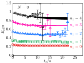
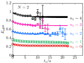
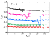
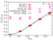
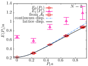
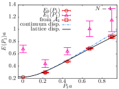
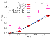
Figure 1: The spectral content of pion two-point functions in $N=0,2,4,8$ quark flavors from left to right. (Top) The effective mass from pion two-point function at different momenta (different colored symbols) shown as a function of source-sink separations $t_{s}/a$ in lattice units. The bands are the expected effective mass from two-state fits to the two-point function. (Bottom) The dispersion relation between ground state (red circles) and the first excited state (purple triangle) energy on boosted momentum is shown. For comparison, the expected single particle dispersion in the continuum (blue dashed curve) and on the lattice (black curve) are shown. The ground state pion energy extracted from axial-vector ${\cal A}_{1}$ correlator are also shown at non-zero momenta.

The contractions for the above three-point function were performed using the sequential-source trick (c.f., appendix of Izubuchi et al. (2019) for details relevant to the bilocal operator) to take care of the necessary Fourier summation over two-dimensional time-slice at the sink. It should be noted that, similar to the $u-d$ three-point function of the pion in 3+1 dimensions, the three-point function is purely real at all $P_{1}$. Also, there are no fermion-line disconnected pieces; this comes non-trivially at finite lattice spacing, by the parity invariance of the action which guarantees that $\langle{\rm Tr}(\not{D}_{w}^{-1})\rangle=-\langle{\rm Tr}({\not{D}^{\dagger}_{w}}^{-1})\rangle$. If one used 2+1 dimensional overlap fermions Karthik and Narayanan (2016b), the cancellation of disconnected piece would have been on each configuration.

V.5 Pion decay constant computations

We will quantify the presence of infrared scale in the system using the pion decay constant, $F_{\pi}$, defined in Eq. (4). We extracted this matrix element using the axialvector-pion two-point function (c.f., Mastropas and Richards (2014)),

$$C_{\pi-{\cal A}}(t_{s})\equiv\left\langle{\cal A}_{3}(\mathbf{x}_{0},t_{s})\pi^{\dagger}_{S}(\mathbf{P}=0,0)\right\rangle;\ {\cal A}_{3}(x)=\overline{d}(x)\sigma_{3}u(x).$$ (37)

The pion source was optimally Wuppertal smeared, whereas the current is constructed out of point quark operators. We will describe the analysis of the two-point function leading to $F_{\pi}$ in a subsequent section.

VI Analysis of correlator data to obtain the pion bilocal matrix element & $F_{\pi}$

VI.1 The spectral content of pion correlator

The two point function in Eq. (32) gives information on the spectrum of states contributing to the pion quantum number, that we will use to extract the ground state boosted bilocal matrix element. In the top panels of Fig. 1, we have shown the effective masses for the pion at all flavors as a function of source-sink separation $t_{s}$, both in lattice units. For each flavor, the effective masses at the five momenta are shown by the different symbols. First, one can see that the ground state displays a well defined plateau for all $N$, even for $N=8$, thereby demonstrating the effectiveness of gapping the spectrum by finite valence quark mass and volume even in the otherwise conformal infrared theories. We can see that the value of the ground state mass has been tuned well to be $\approx 0.227a$ in all the theories, which corresponds to $0.53g^{2}$ physical mass. The smallest $t_{s}$ from where one can see a well-defined plateau, at least for the smallest three momenta, increases with momenta due to the decreasing gap with the excited state with the boost. However, we have tuned the Wuppertal smearing and quark boost parameters precisely to reduce the amplitudes of the excited state as best we could, and the any observed deviation from the plateau at smaller $t_{s}$ was the best we could reduce it to, without compromising on the noise at larger $t_{s}$. Since the range of $t_{s}$ that we will use to analyze the three-point function falls in the small $t_{s}$ region without the plateau, we need to understand the spectral content of $C_{\rm 2pt}$ better.

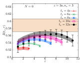
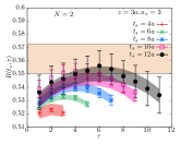
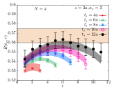
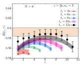
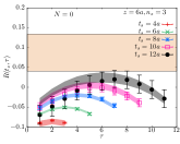
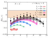
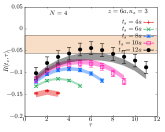
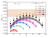
Figure 2: The estimation of matrix element $h_{00}(z_{1},P_{1})$ by the two-state fits to the ratio, $R(t_{s},\tau)$. Some sample fits to the operator insertion point, $\tau$, and the source-sink separation, $t_{s}$, dependence of $R$ are shown in the different panels; the top panels are at $z_{1}=3a$ and the bottom ones are $z_{1}=6a$, at a momentum of $n_{1}=3$. For each $z_{1}$, the panels from left to right are from different number of flavors.

We take the spectral decomposition of $C_{\rm 2pt}$,

$$C_{\rm 2pt}(t_{s};P_{1})=\sum_{i=0}^{N_{\rm state}-1}|A_{i}|^{2}\left(e^{-E_{i}(P_{1})t_{s}}+e^{-E_{i}(P_{1})\left(aL_{3}-t_{s}\right)}\right),$$ (38)

and truncate it at $N_{\rm state}=2$, which is referred to as the two-state ansatz. We found that this is enough to describe the behavior of $C_{\rm 2pt}(t_{s})$ for all the $P_{1}$ used, even starting from $t_{s}=2a$ and be able to reproduce the value of ground state $E_{0}$, as obtained from one-state fit with the minimum $t_{s}>10a$. The uncertainly bands for the effective mass curves for the different $P_{1}$ based on the two-state fits over the range $t_{s}\in[3a,24a]$ are also shown in Fig. 1 along with the data. The quality of the fits are seen to be good, which is also reflected in $\chi^{2}/{\rm dof}\approx 1$ for the fits. We repeated the two-point function computation using $\langle{\cal A}_{1}(0){\cal A}_{1}(t_{s})\rangle$ correlators also; at $P_{1}=0$, this gives the mass of the axial-vector meson, but at non-zero momentum the lowest mass comes from the pion due to the non-zero overlap $\sim P_{1}F_{\pi}$ with the lighter pion state. Thus, at non-zero momenta this gave a cross-check on the determined ground-state values of the pion.

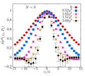
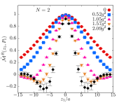
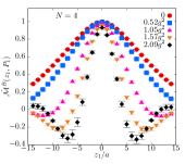
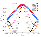
Figure 3: The matrix elements at $N=0,2,4,8$ (left to right) obtained by extrapolation are shown as a function of quark-antiquark separation $z_{1}/a$. The different colored symbols correspond to different fixed momenta $P_{1}$, which are shown in the legend in units of gauge coupling $g^{2}$.

In the bottom panels of Fig. 1, we have shown the best fit values of the ground state energy $E_{0}$ and the first excited state $E_{1}$ as a function of boosted momentum $P_{1}$. The different panels are again for the five different $N$. We have compared the data for $E_{0}(P_{1})$ with the curves for the single particle dispersion in the continuum, $E_{0}(P_{1})=\sqrt{P_{1}^{2}+{M_{\pi}^{\rm val}}^{2}}$, shown as the blue dashed curves. There is a slight discrepancy which increases with $P_{1}$, as $P_{1}a\approx 1$ at the largest momentum used. We can understand this by, instead comparing the data with the lattice dispersion, $\cosh(E_{0}(P_{1})a)=\cosh(M_{\pi}^{\rm val}a)+1-\cos(P_{1}a)$. This lattice single particle dispersion curve is shown as black continuous curve in the figures. The nice agreement tells us that there are possible lattice corrections at the level of $3-4\%$ at the highest momenta, which can be reduced in the future by going to much finer lattices. But this effect will persist for all the $N$, and therefore, we do not expect this to affect variations as a function of $N$ that we are interested in. As a cross-check, we have also shown the values of ground-state masses of pion as extracted from the axial-vector ${\cal A}_{1}$ correlator at non-zero momenta, which can be seen to agree with the values from the simple pion correlator. While the slight disagreement with the dispersion curve at higher momenta are understood as lattice spacing effect, a slight disagreement at the level of 4% is also seen at the smallest non-zero momentum corresponding to $n_{1}=1$ for $N=4$ and 8. This tells us that the valence pion mass for the near-conformal and conformal theories mildly originate from aspect-ratio($\zeta$)-dependent $1/\ell$ effect that we described in Section III, in spite of our effort to use somewhat larger value of valence quark mass. As the pion is boosted, the aspect ratio in the boosted frame decreases, and causes the observed small discrepancy at the smallest non-zero momentum. At the larger momentum, these aspect-ratio variations are not important as the leading $E\propto P_{1}$ relativistic dependence takes over. Therefore, as a precaution, we will avoid using $n_{1}=1$ momentum in our analysis of three-point function to avoid systematic effects. In a future computation, we aim to rectify this by using lattices with $\zeta<1$.

In the next section, we will use the extracted energies and amplitudes in the two-point function to determine the ground state bilocal matrix element from the three-point functions.

VI.2 The extraction of the pion bilocal matrix element from three-point function

The required ground state matrix element of the bilocal operator can be obtained from the spectral decomposition of the three-point function,

$$C_{\rm 3pt}(t_{s},\tau;P_{1},z_{1})=\sum_{i,j=0}^{N_{\rm state}-1}A_{i}^{*}A_{j}h_{ij}(z_{1},P_{1})e^{-E_{i}(t_{s}-\tau)-E_{j}\tau},$$ (39)

with the amplitudes $A_{i}$ and energies $E_{i}$, being the same as obtained from the two-point function analysis. The matrix elements are the terms $h_{ij}=\langle E_{i},P_{1}|{\cal O}_{\sigma_{3}}(z_{1})|E_{j},P_{1}\rangle$. Therefore, the leading term $h_{0,0}$ is the required ground state matrix matrix element $\langle\pi;P_{1}|{\cal O}_{\sigma_{3}}(z_{1})|\pi;P_{1}\rangle$.

We extracted this leading term by fitting the $t_{s},\tau$ dependencies of the actual $C_{\rm 3pt}$ data at various fixed $z_{1}$ and $P_{1}$ using the above spectral decomposition truncated to $N_{\rm state}=2$ (since we found that $N_{\rm state}=2$ was able to describe the corresponding two-point function well even from small $t_{s}\approx 2-3a$). In practice, we constructed the ratio,

$$R(t_{s},\tau)\equiv\frac{C_{\rm 3pt}(t_{s},\tau)}{C_{\rm 2pt}(t_{s})},$$ (40)

with the $P_{1}$ and $z_{1}$ arguments being the same for both numerator and denominator, and hence notationally suppressed above. We then fitted $R(t_{s},\tau)$ using the ratio of expressions in Eq. (39) and Eq. (38), with $h_{ij}$ as the fit parameters. We took the values of the amplitudes $|A_{i}|$ and energies $E_{i}$ from the two-state fit analysis of $C_{\rm 2pt}$ with the fit range over $t_{s}\in[3a,24a]$. We used these $(A_{i},E_{i})$ from the same Jack-knife blocks as used for the three-point function analysis. We performed these fits over $\tau\in[2a,t_{s}-2a]$ to reduce larger excited state effects for insertion closer to source and sink. Further, we used all the data for $t_{s}/a\in[6,8],[6,10],[6,12],[6,12],[6,10]$ for momenta $n_{1}=0,1,2,3,4$ respectively; we skipped $t_{s}=10a,12a$ for $n_{1}=0$ in order to reduce the 0.4% lattice periodicity effect due to the smaller $E_{0}$, and similarly we skipped only $t_{s}=12a$ for the larger $n_{1}=1$ momentum. We did not used $t_{s}=12a$ for $n_{1}=4$ as the two-point function for $t_{s}>10a$ was very noisy. While the extrapolated values were insensitive to changes in fitting windows, we kept the fit systematic fixed for all $N$ so that even if there is any unnoticed systematic error, it is unlikely to affect the overall variations in the data as a function of $N$, which is our interest in this paper. Such a two-state fit to the ratio $R$ resulted in good fits for all $z_{1}$ and $P_{1}$.

Some sample data for $R$ along with the results from the fits are shown in Fig. 2 for the case of momentum $n_{1}=3$. The top and the bottom panels are for fixed $z_{1}=3a$ and $6a$ respectively, with the different $N$ shown in the different columns. The fits, shown as bands, agree with the data well for all $N$, and the extrapolated value is shown as the horizontal band. The ground state matrix element ${\cal M}^{B}(z_{1},P_{1})=h_{00}(z_{1},P_{1})$ so extracted, are shown as a function of $z_{1}/a$ in Fig. 3; with each panel for different $N$, and in each panel, the data for different momenta differentiated by color and symbols. The data has not been symmetrized by hand with respect to $z_{1}$ and $-z_{1}$, so as to show that the symmetry emerges automatically, which is a simple cross-check on the computation. The local matrix element corresponding to $z_{1}=0$ should be precisely be 1 if we had used an exact conserved current on the lattice, which we have not. So, one sees the matrix element at $z=0$ to be slightly below 1 at $z=0$ and this difference with 1 increases with larger momentum; we found this lattice spacing effect to be of the kind $(aP_{1})^{2}$, which was also seen in 3+1 dimensional computation Gao et al. (2020). We will see that such effects are nicely canceled by an overall normalization such that $z=0$ matrix elements are exactly 1; this is justified since the information on the PDF comes from the variations in $z_{1}$ and $P_{1}$, and not by a fixed overall normalization.

VI.3 Determination of pion decay constant

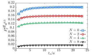
Figure 4: The determination of pion decay constant $F_{\pi}$. The data points are the effective $F^{\rm eff}_{\pi}(t_{s})$ as determined from the $\langle{\cal A}_{3}\pi\rangle(t_{s})$ correlator, and the curves are fits to $F_{\pi}+Ae^{-\delta mt_{s}}$.

We determined the pion decay constant through the spectral decomposition of the correlator $C_{{\cal A}-\pi}$ in Eq. (37) as,

$$C_{{\cal A}-\pi}(t_{s}) = \frac{-F_{\pi}}{\sqrt{2M_{\pi}^{\rm val}}}M_{\pi}^{\rm val}A_{0}\left(e^{-M_{\pi}^{\rm val}t_{s}}-e^{-M_{\pi}^{\rm val}(aL_{3}-t_{s})}\right)$$ (42)

$$\qquad+A^{\prime}e^{-E^{\prime}t_{s}}+\ldots,$$

which follows from Eq. (4) with $\mu=3$. The factor of $\sqrt{2M_{\pi}^{\rm val}}$ is to convert the lattice normalization of state vectors to the relativistic one used in defining $F_{\pi}$. The factor $A_{0}$ is the amplitude $\langle 0|\pi^{S}|\pi\rangle$, which we take from the smeared-smeared pion two-point function at zero momentum; we only determine the magnitude of $A_{0}$, and therefore we are assuming there is no phase in $A_{0}$. The correlator is anti-periodic in the $t$-direction, which can be seen by a rotation in the $xt$-plane; taking $(x_{1},x_{2},x_{3})\to(-x_{1},x_{2},-x_{3})$ along with $u,d\to\sigma_{2}u,\sigma_{2}d$. The excited state contributions captured by $e^{-E^{\prime}t_{s}}$. We fit the above functional form along with a subleading excited state contribution to the $C_{{\cal A}-\pi}(t_{s})$ correlator to determine $F_{\pi}$. Such fits worked well even starting from $t_{s}=2a$ with the fitted value of $F_{\pi}$ independent of the fit range. In Fig. 4, we show an effective $F_{\pi}^{\rm eff}(t_{s})$ obtained by inverting right-hand side of Eq. (42) without excited state term to get a $t_{s}$ dependent value of $F_{\pi}$. The curves in the plot are the expectations for $F_{\pi}^{\rm eff}(t_{s})$ from the excited state fits, which can be seen to perform well. From this analysis, we find $F_{\pi}a^{0.5}=0.200(1),0.1574(7),0.1249(4),0.0164(1)$ for $N=0,2,4,8$ in lattice units.

VII Results

We will present the results in the following logical order; first, we will explain how we measure the presence of infrared scale, by which we establish that the infrared scales are indeed depleted as a function of number of massless fermion flavors $N$. Then, we will infer the Mellin moments of the PDF and reconstruct the PDF based on a two-parameter model, and see how the PDF related quantities change as a function of $N$. This induces a correlation between the infrared scale and the PDF parameters, which we look for.

VII.1 The depletion of infrared scales

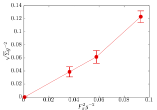
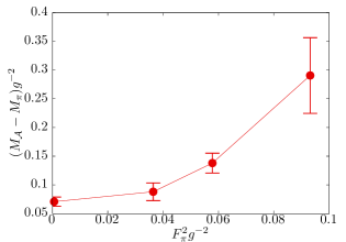
Figure 5: The changes to the infrared scales when the number of massless quark flavor is changed. (Top panel) the quark condensate as a function of decay constant, both implicitly depending on the number of quark flavors. (Bottom panel) a similar plot showing how the mass gap between the pion and the axial vector changes as a function of decay constant.

For the $N=0$ pure-gauge theory, the confining infrared can simply be characterized by the string-tension, which takes a value $\sqrt{\sigma}=0.335g^{2}$ for the SU(2) theory Teper (1999). For theories with non-zero $N$, string-tension is not a good parameter to use; instead we use the condensate $\Sigma$ and the decay constant $F_{\pi}$. In a previous study with R. Narayanan Karthik and Narayanan (2018), we measured the scalar condensate $\Sigma$ that breaks the Sp$(N)$ global flavor symmetry, as a function of $N$ in the massless limit of the theory. For this, we compared the finite-size scaling (FSS) of the low-lying eigenvalues, $\lambda_{i}\propto z_{i}\Sigma^{-1}\ell^{-3}$ behavior of the eigenvalues in an $\ell^{3}$ box, where the proportionality constant $z_{i}$ are the eigenvalues of the random matrix model from the non-chiral Gaussian Orthogonal Ensemble Verbaarschot and Zahed (1994), which shares the same symmetries as the Dirac operator coupled to SU(2) gauge field in 2+1 dimension. The coefficient $\Sigma$ is the condensate in the massless limit. We found non-zero $\Sigma/g^{4}=0.0152(22),0.0038(12),0.0025(7)$ and $0.0(6)10^{-6}$ for $N=0,2,4,8$ flavor respectively. The $N=8$ and 12 theories were instead likely to be infrared conformal with non-trivial mass anomalous dimensions $\gamma_{m}=0.38(8)$ and $\gamma_{m}=0.48(6)$ respectively; that is, the Dirac eigenvalues displayed its FSS as $\lambda_{i}\propto\ell^{-\gamma_{m}-1}$ rather than an $\ell^{-3}$ FSS expected from SSB. Here, we should remark that we found that it was also possible to describe the eigenvalue FSS in the $N=4$ theory assuming a rather large $\gamma_{m}=0.6$ along with additional subleading $1/\ell$ FSS corrections; however, in light of the results on $F_{\pi}$ in this work, it appears that the $N=4$ theory indeed is more likely to be scale-broken in the IR. The $F_{\pi}$ we determined here are at finite volume and finite valence pion mass, but it cannot change the non-zero $F_{\pi}$ result for $N=4$ because of the following. One should notice that the very small $F_{\pi}^{2}=6\times 10^{-4}g^{2}$ for $N=8$ is most likely to arise due to finite volume and valence quark mass, and hence it gives the typical correction to $F_{\pi}$ due to these effects; the value of $F_{\pi}$ for $N=4$ theory is $F_{\pi}^{2}=0.036g^{2}$, which is much larger than those typical corrections, and hence justifying our inference about the IR fate of $N=4$. Thus, our current understanding about the IR fate of many-flavor SU(2) gauge theory is that $N=0,2,4$ are likely to be scale-broken, whereas the $N\geq 8$ are likely to be conformal in the IR.

The depletion of all the infrared scales due to the monotonic reduction in condensate is quite apparent. To see this, we plot different mass-scales, all appropriately casted to have mass-dimension 1, one versus another. In the top panel of Fig. 5, we plot the mass-scale from condensate, $\sqrt{\Sigma}/g^{2}$, as a function of another scale, $F_{\pi}^{2}/g^{2}$. The two seem to be almost directly proportional. Another infrared scale one could use is the mass-gap, $M_{\cal A}-M_{\pi}^{\rm val}$ between the pion and the axial-vector meson. In the bottom panel of Fig. 5, we correlate this mass-gap with $F_{\pi}^{2}$. Again, it is clear than the mass-splitting also shrinks with the other diminishing, perhaps a more fundamental scale, $F_{\pi}$. The mass-splitting does not go to zero even for $N=8$ most likely because of the finite fixed volume and the quark mass. The one-to-one positive correlation between the infrared scales also suggests that we can now make the number of flavors implicit, and simply ask for the effect of reducing one infrared scale on another, as done in Fig. 5. As one would have expected, a factor reduction in $F_{\pi}$ induces a reduction in other scales by a similar factor. We now apply this perspective to quark structure of pion, where the effect is not obvious.

VII.2 Response of the pion PDF to changes in infrared

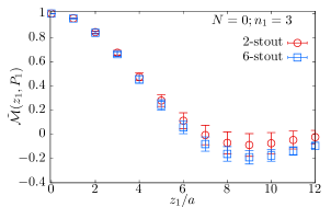
Figure 6: A cross-check that at least an application of small number of Stout smearing to the Wilson-line connecting quark-antiquark is harmless. The pion bilocal matrix element at $n_{1}=3$ momentum in $N=0$ theory with 2-stout and 6-stout smeared Wilson line insertions are compared and shown to be consistent once the ratio is taken.

The central object in our analysis of PDF is the equal time bilocal matrix element $\tilde{\cal M}(z_{1},P_{1})$ in Eq. (23), formed by taking ratios of the matrix elements ${\cal M}^{B}(z_{1},P_{1})$ that we obtained directly from the three-point function analysis. We formed these ratios to remove the presence of $\exp(-c^{\prime}g^{2}z_{1})$ behavior due to the Wilson-line which is present in the definition of the bilocal operator, and hence ensure a better description by the OPE. In Appendix A, we describe features of ${\cal M}^{B}$ itself, and here we proceed with using the improved $\tilde{\cal M}$. Through its OPE in Eq. (22), $\tilde{\cal M}$ contains the leading twist terms that relate to the pion PDF as well as contribution from operators with higher-twist, which could have interesting physics in their own right, but for our purposes here are contaminations. We can distill the leading-twist PDF terms in a practical lattice computation, when $z_{1}$ is small and $P_{1}$ is large, so that one has a finite range of $z_{1}P_{1}$ which can simply be described the lead-twist part of the OPE in the analysis. Before going further, we need to first make sure that the ratio in Eq. (23) indeed cancels any remnant non-perturbative $z_{1}$-dependent factor from the usage of Wilson line in the operator. For this, we performed the computations of $\tilde{\cal M}(z_{1},P_{1})$ with 2-stout and 6-stout smeared Wilson lines for a sample case with $n_{1}=3$ momentum in the $N=0$ theory. The results from the two are compared in Fig. 6, where one can see a good agreement between the two, giving confidence that the results are not stout smearing dependent, at least for few steps of it. The results get less noisier when number of stout smearing steps increases, but we use 2-stout in order to be conservative.

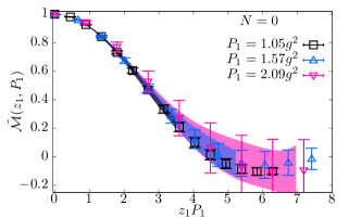
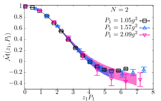
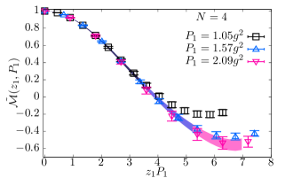
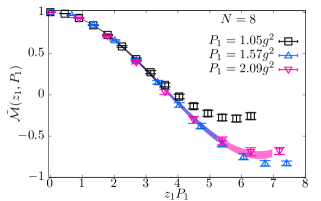
Figure 7: The pion bilocal quark bilinear matrix elements, $\tilde{{\cal M}}(z_{1},P_{1})$ from $N=0,2,4$ and 8 flavor theories are shown in the four panels. In each panel, the matrix elements from $P_{1}=1.05,1.57,2.09g^{2}$ are put together and shown as a function of $z_{1}P_{1}$. The color and symbols differentiate the data at fixed $P_{1}$. The bands are the expectations for $\tilde{{\cal M}}(z_{1},P_{1})$ based on the fits to the leading twist expression in Eq. (43). The bands extend over points included in the fit.

We perform two types of analysis on $\tilde{\cal M}$, namely, a model-independent determination of the even moments of the valence quark PDF, and secondly, by model-dependent reconstruction of $x$-dependent PDF (even the model-independent determination can have additional systematic dependences on the modelling of higher-twist effects, lattice corrections, fit ranges, etc). For both the ways, the starting point is the working version of the leading twist OPE in Eq. (22) with some unknown higher-twist $z_{1}^{2}$ corrections, namely,

$$\tilde{\cal M}(z_{1},P_{1})=\frac{1+\left[\sum_{k=1}^{N_{\rm max}}(-1)^{k}\frac{(z_{1}P_{1})^{2k}}{(2k)!}\langle x^{2k}\rangle_{v}\right]+bz_{1}^{2}}{1+bz_{1}^{2}}.$$ (43)

We have rewritten leading twist part of Eq. (22) in a different form above so that is clear that $\langle x^{0}\rangle=1$, $\tilde{\cal M}$ is purely real and that only even valence PDF moments $\langle x^{2k}\rangle_{v}$ appear. These are very specific properties of $\tilde{\cal M}$ for a pion in 2+1 as well as 3+1 dimensions. We have modelled the higher-twist effect in such a way that the individual matrix elements ${\cal M}(z_{1},P_{1})$ and ${\cal M}(z_{1},0)$, that enter the ratio for $\tilde{\cal M}(z_{1},P_{1})$, suffer from a momentum independent leading $bz_{1}^{2}$ higher-twist correction, which leads to the presence of similar term in the numerator and demoninator of Eq. (43). Effectively, this causes a leading $(z_{1}P_{1})^{2}z_{1}^{2}$ correction term in the ratio. The upper-cutoff of the sum $N_{\rm max}$ is infinity but for practical implementation, we need to work with smaller $N_{\rm max}$ since the data is only sensitive to some smaller powers $k$. Here, the moments of the PDF are the unknowns we are interested it, but we will also fit the parameter $b$ to effectively take care any higher twist $g^{2}z,F_{\pi}^{2}z$ corrections, and also any target mass corrections. We also tried adding lattice corrections of the form $(aP_{1})^{2}$ to the above functional form of OPE Gao et al. (2020) for $z_{1}>0$, but such terms were found to be unnecessary and consistent with zero well within errors. Therefore, we do not present such an analysis here. Since this work is at a fixed lattice spacing, any overall $O(a)$ correction that is independent of $z_{1}$ and $P_{1}$ cannot quantified, but a correction such as $(az_{1})^{2}$ can be absorbed with the $z_{1}^{2}$ correction that we have already added.

In any method of analysis, we need to choose the range of $z_{1}$ and $P_{1}$ carefully, since we will not be taking either $z_{1}\to 0$ or $P_{1}\to\infty$ limits, and instead we will simply be fitting the data which spans a finite range of $z_{1}$ and $P_{1}$. First, we will work with momenta $P_{1}/g^{2}\geq 1$ to make sure that for a given separation $z_{1}$, a term like $(P_{1}z_{1})^{k}$ is larger than a similar order term $(g^{2}z_{1})^{k}$. This leaves the momenta corresponding to $n_{1}=2,3,4$. Through this choice, we are also guaranteed that $M_{\pi}^{\rm val}/P_{1}$ and $F_{\pi}^{2}/P_{1}$ corrections would also be controlled. For the range of quark-antiquark separation $z_{1}$, we have two choices; we might want $z_{1}g^{2}<1$ or $z_{1}F_{\pi}^{2}<1$, where the first factor is simply due to the superficial dimensional scale in the system and the second is the natural infrared scale. We assume that the superficial scale will arise simply due the $\exp(-cg^{2}z)$-type Wilson-line term which we find to be nicely canceled in the ratio $\tilde{\cal M}$. Due to the natural infrared scales being at least a factor $10$ smaller than $g^{2}$ for $N=0$, and even smaller for larger $N$, even a usage of $z=10a$ will only lead to $F_{\pi}^{2}z=0.4$ in this system. Thus, we restricted ourselves to $z\in[a,8a]$ and change the maximum $z_{1}$ to $6a$ and $10a$ to check for the robustness of results. The justifications for the used ranges of $z_{1},P_{1}$, will also bear out in the data.

VII.2.1 Model-independent inferences

In the model independent analysis Karpie et al. (2018); Gao et al. (2020), we first fit Eq. (43) to $\tilde{\cal M}(z_{1},P_{1})$ data over the specified range of $z_{1}$ and $P_{1}$ with the even moments $\langle x^{2k}\rangle_{v}$ being the fit parameters. In addition, we also fitted the high-twist parameter $b$ to take care leading higher twist effects; but their values were consistent with zero, and when we performed the fits without the higher-twist corrections, the results were consistent with the one including it. Here, we keep this correction nonetheless. Since the valence quark PDF is positive (since the anti-$u$ quark and $d$ quark arises only radiatively in $u\overline{d}$ pion , whereas the $u$ quark is present at tree-level itself), it imposes a set of inequalities to be satisfied by the moments as discussed in Gao et al. (2020); with the important one being $\langle x^{k}\rangle_{v}<\langle x^{m}\rangle_{v}$ for $k>m$. We imposed these constraints in the fit using the methods discussed in Gao et al. (2020). With such constraints, one can add as many moments, $N_{\rm max}$, in the analysis without over-fitting the data, except that it will result in many of the higher-moments, which the data is not sensitive, to converge to zero. We found that $N_{\rm max}=5$ was sufficient to describe the data in the range we fitted, as we describe below.

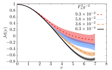
Figure 8: The effect of reduction in $F^{2}_{\pi}$ on the bilocal matrix element (Ioffe-time distribution) ${\cal M}(\nu)$ is shown. The bands are inferred from the fits to lead-twist expression in Eq. (43) and taking its $z_{1}\to 0,P_{1}\to\infty$ limit at fixed $P_{1}z_{1}=\nu$. The matrix element is shown as a function of $\nu=P^{+}\xi^{-}$ (Ioffe time). The different colored bands are at different $F_{\pi}^{2}g^{-2}$.

In Fig. 7, we show the data for $\tilde{\cal M}(z_{1},P_{1})$ as a function of $z_{1}P_{1}$; the data from different fixed pion momenta $P_{1}$ are differentiated by the colored symbols. The four different panels show the data from $N=0,2,4,8$ flavors. The data can be seen to fall on almost universal curves as a function of $z_{1}P_{1}$, which demonstrates the dominance of the lead-twist part, as is essential for this work. As seen by the early peeling-off of $P_{1}=1.05g^{2}$ data from the higher momenta data beyond $P_{1}z_{1}>4$ for $N=4,8$ suggests that the leading twist dominance works better for $N=0$ than for $N=8$. This could be because the natural higher-twist scale in the broken phase is $F_{\pi}^{2}$ which is smaller than the natural scale corrections $g^{2}z$, and the finite-box scale, $z/\ell$, which could be important in the conformal phase. However, for the range of $z_{1}=6a,8a,10a$, this ensuing higher twist effect is less important even for $P_{1}=1.05g^{2}$, and definitely not important for higher momenta. This justifies our choices of fit ranges and the reasoning we presented before. The data gets increasingly precise with increasing $N$ because the fluctuations in the gauge field decreases roughly as $1/\sqrt{N}$ for larger $N$. The bands of various colors in Fig. 7 are the expectations for ${\cal M}(z_{1},P_{1})$ from the best fits from the analysis; the colors match the corresponding color for the momenta for the data. The bands cover the range of $P_{1}z_{1}$ for each $P_{1}$ for a fixed range of $z_{1}$ up to $8a$, and for $P_{1}=1.05g^{2}$ this range is within the point where the higher twist effects start becoming visible at this lower momentum. The quality of fits are very good with resulting $\chi^{2}/{\rm dof}\approx 0.6$ to 0.8.

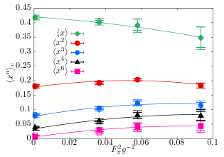
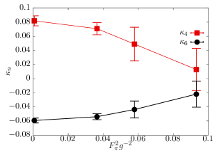
Figure 9: (Top) The correlation between decay constant and the valence PDF moments. The filled symbols are obtained from model-independent fits and the open ones from model-dependent PDF ansatz fits. For model-independent fits only the even moments are directly obtained, whereas the odd moments $\langle x\rangle_{v}$ and $\langle x^{3}\rangle_{v}$ were obtained indirectly by definition in Eq. (46). The curves are quadratic fits in order to interpolate the data. (Bottom) The correlation between decay constant and the cumulants $\kappa_{4}$ and $\kappa_{6}$ of $u-d$ PDF.

In Fig. 8, we have taken the results of the above model-independent fits to $\tilde{\cal M}(z_{1},P_{1})$ and extracted the light-front bilocal matrix element, ${\cal M}(\nu)$, which is the Ioffe-time Distribution (ITD). As we discussed, the variation of infrared scales with $N$, induces a direct infrared scale dependence of various quantities. Therefore, in Fig. 8, we have shown the ITD dependence on the decay constant. This is the main result in this paper, which we will process further and look at from various angles. As the infrared scale-breaking is made stronger, as reflected in $F_{\pi}$, the corresponding valence quark ITD starts peeling off from the large-$N$ conformal curve at shorter and shorter $\nu$. In this process, however, the ITD remains almost universal up until $\nu\approx 3$. This tells us that the lowest non-zero $u-d$ moment, $\langle x^{2}\rangle_{u-d}=\langle x^{2}\rangle_{v}$, must remain quite insensitive to the scale changes. Thus, the effect of scale-breaking seems to be encoded in the fall-off rate of the ITD for $\nu>3$ with an almost fixed lowest even moment. We can infer simply that this will reflect in the low-$x$ behavior, which is typically modeled as a Regge-type $x^{\alpha}$ behavior, and also in the large-$x$, $(1-x)^{\beta}$ behavior of the underlying valence PDF. This is because, the tail of the ITD typically carries information on the small-$x$ asymptotic of the PDF, whereas given the inference that the lowest moment will be almost fixed, will induce a variation in $\beta$ as well via the implicit relation $\langle x^{2}\rangle_{v}(\alpha,\beta,\ldots)$, with $(\alpha,\beta,\ldots)$ being the parametrization of the shape of the PDF.

In the top panel of Fig. 9, we have plotted the $F_{\pi}^{2}$ dependence of the first three even moments $\langle x^{2}\rangle_{v},\langle x^{4}\rangle_{v},\langle x^{6}\rangle_{v}$, as obtained directly from the model-independent analysis discussed above, using the closed symbols. Since we can directly get only the even valence moments, we infer the odd moments from $\langle x^{2}\rangle_{v}$ and $\langle x^{4}\rangle_{v}$ by assuming a two-parameter PDF ansatz,

$$f_{v}(x)={\cal N}x^{\alpha}(1-x)^{\beta},$$ (44)

with normalization ${\cal N}$ to ensure $\langle x^{0}\rangle_{v}=1$, and simply solve for $\alpha$ and $\beta$ through the two equations,

$$\frac{\Gamma(3+\alpha)\Gamma(2+\alpha+\beta)}{\Gamma(1+\alpha)\Gamma(4+\alpha+\beta)} = \langle x^{2}\rangle_{v},$$ (45)

$$\frac{\Gamma(5+\alpha)\Gamma(2+\alpha+\beta)}{\Gamma(1+\alpha)\Gamma(6+\alpha+\beta)} = \langle x^{4}\rangle_{v}.$$ (46)

Through this we get $\langle x^{2k-1}\rangle_{v}(\alpha,\beta)$ by this semi-model-dependent analysis. As a cross-check, this procedure also predicts the even moment $\langle x^{6}\rangle(\alpha,\beta)$, which we found to agree well with the actual value we obtained in the model-independent analysis. These odd moments $\langle x\rangle_{v}$ and $\langle x^{3}\rangle_{v}$ are also shown in Fig. 9. The inferred value of $\langle x\rangle_{v}$, the fraction of pion mass carried by a valence quark, seems to be $\approx 0.35$ in $N=0$ theory and increases to $\approx 0.45$ as $F_{\pi}$ decreases to zero. Thus, even in the strongly confined regime of 2+1 dimensional SU(2) QCD, about 30% of pion mass is carried by gluons and sea quarks, which one might want to contrast with the 3+1 dimensional QCD where this fraction is about $\approx 55$%, at a scale of $3$ GeV Barry et al. (2018), and decreases further as the scale approaches $\Lambda_{\rm QCD}$. Thus, it might be that the scale-independent value of moments in 2+1 dimensions has to be compared with PDFs in 3+1 dimensions determined at typical non-perturbative hadronic scales to serve as good analogues. We interpolated the data with a quadratic in $F^{2}_{\pi}g^{-2}$, which are shown as the curves in Fig. 9. It is quite striking how the individual moments themselves weakly depend on $F_{\pi}$. One should contrast this behavior with the commensurate dependence of other IR quantities to this decrease in $F_{\pi}$. As we inferred from the ITD itself, $\langle x^{2}\rangle_{v}$ seems to be the least sensitive to changes in $F_{\pi}$.

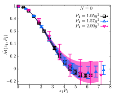
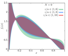
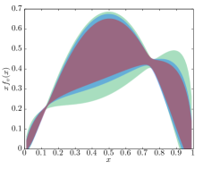
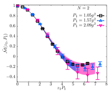
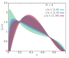
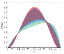
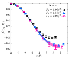
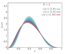
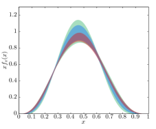
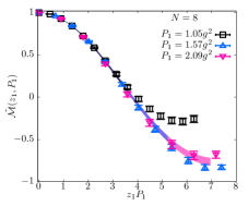
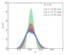
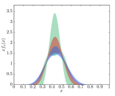
Figure 10: Reconstruction of valence PDF, $f_{v}(x)$, by fits to two-parameter ansatz. The left panels show the fits (bands) to the bilocal matrix element $\tilde{\cal M}(z_{1},P_{1})$ (points) via leading-twist expression in Eq. (43). The middle panels show the inferred valence PDF, $f_{v}(x)$. The different colored bands correspond to different fit ranges $[0,z_{1}]$. The right panels show $xf_{v}(x)$. Top to bottom are $N=0,2,4,8$ theories respectively.

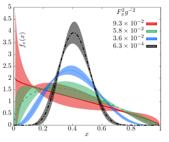
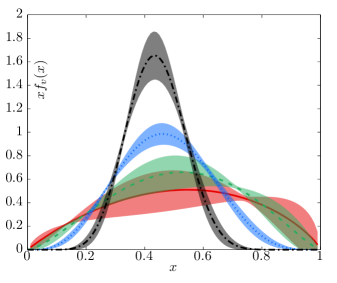
Figure 11: (left) The reconstructed valence pion PDFs, $f_{v}(x)$, and (right) their corresponding momentum distribution, $xf_{v}(x)$ are shown as a function of pion decay constant that characterizes the vacuum of different $N=0,2,4,8$ flavor theories.

It is the observables that dictate the shape of the full $x$-dependent PDF that are quite sensitive the infrared rather than the moments themselves. One such observable is the $\log$-derivatives Gao et al. (2020) of moments $\beta_{\rm eff}(k)=-1-\partial\log(\langle x^{k}\rangle_{v})/\partial\log(k)$ which approaches the large-$x$ exponent $\beta$ for $k\to\infty$. As explained in Gao et al. (2020), we define the discretized version of the effective $\beta$ for any $k$ as

$$\beta_{\rm eff}(k)=\frac{\langle x^{k-2}\rangle_{v}-\langle x^{k+2}\rangle_{v}}{\langle x^{k}\rangle_{v}}\frac{k}{4}-1.$$ (47)

Using $k=4$, we find $\beta_{\rm eff}$ for $N=0,2,4,8$ to be $0.8(5),1.0(4),2.1(2),3.3(2)$ respectively. As expected, this quantity shows a sharp increase as the theory moves from being strongly confined to being infrared conformal. The $u-d$ PDF, $f_{u-d}(x)$ being a positive quantity and having a probabilistic interpretation, also admits the canonical shape observables, cumulants $\kappa_{n}$,

$$\kappa_{n} \equiv \frac{\partial^{n}}{\partial s^{n}}\log\left(\int_{-1}^{1}f_{u-d}(x)e^{sx}dx\right)\bigg{|}_{s=0}\qquad{\rm with},$$ (48)

$$\kappa_{4} = \langle x^{4}\rangle_{v}-3\langle x^{2}\rangle_{v}^{2},$$ (49)

$$\kappa_{6} = \langle x^{6}\rangle_{v}-15\langle x^{2}\rangle_{v}\langle x^{4}\rangle_{v}+30\langle x^{2}\rangle_{v}^{3}.$$ (50)

Using the model independent estimates of the even moments up to $\langle x^{6}\rangle_{v}$, we find the fourth and sixth cumulants, $[\kappa_{4},\kappa_{6}]$, for $N=0,2,4,8$ flavors to be [0.01(3), -0.02(2)], [0.05(2), -0.04(1)], [0.071(8), -0.054(4)], [0.02(8), -0.059(4)] respectively. This variation is shown in the bottom panel of Fig. 9, and it can seen to be very sensitive to the IR changes. One could do a similar analysis by including the non-vanishing odd valence moments, but we specifically chose the cumulants of $u-d$ PDF so as to keep the analysis fully model-independent. The aim of this exercise was to point to some good observables of the pion PDF that seem to be sensitive about the IR, and consequently, we were able to deduce simply from the model independent analysis that the shape of the PDF will show sharp changes as the theory morphs. Next, we will see these inferences concretely arise in the reconstructed $x$-dependent valence PDFs.

VII.2.2 Model dependent analysis: PDF reconstruction

Now we reconstruct the $x$-dependent valence PDFs that best describe the real space data for $\tilde{\cal M}(z_{1},P_{1})$. For this we use the two-parameter functional form of the PDF in Eq. (44) that was completely sufficient to describe $\tilde{\cal M}(z_{1},P_{1})$ at all $N$ and in the range of $z_{1}$ and $P_{1}$ described before; in fact, when we tried to make the ansatz more complex by adding subleading small-$x$ terms $x^{\alpha+0.5}$ and $x^{\alpha+1}$, the fits became quite unstable and hence we resort to the simpler two-parameter ansatz. Essentially, the parametrized PDF enters through its corresponding moments $\langle x^{2k}\rangle_{v}(\alpha,\beta)$, that is then input into the leading twist OPE in Eq. (43) to get the best values of $\alpha$ and $\beta$. In the left panels of Fig. 10, we have shown the resulting curves for $\tilde{\cal M}(z_{1},P_{1})$ from such two-parameter fits superimposed on the data. The quality of fits are as good as the one from model-independent fits shown in Fig. 7.

The valence PDFs, $f_{v}(x)$, corresponding to the best fits are shown in the middle panels of Fig. 10, and the rightmost panels are simply the same data replotted as the momentum distribution, $xf_{v}(x)$. We checked that the reconstructed PDFs were robust against variations in the fit ranges by changing the maximum of the fit range from $z_{1}=6a$ to $z_{1}=10a$. These variations are shown as the bands of different colors in the middle and right panels of Fig. 10. Since the data points fall on universal curves well to begin with, the reconstructed PDFs also show almost no variations; so we simply take the estimate with $z_{1}=8a$ for further discussions. It should be noted that the scales in the different panels in Fig. 10 are different, but it is already clear that the PDFs get narrower as $N$ increases. In terms of the exponents $[\alpha,\beta]$ of the PDFs, they change as $[0.0(7),0.8(8)]$, $[0.5(6),1.4(8)]$, $[2.5(6),4.1(8)]$, $[9(2),13(3)]$ for $N=0,2,4,8$ respectively. The values of the large-$x$ exponent $\beta$ for the strongly broken phase for $N=0$ and 2, are the typical value around 1 and 2 as in 3+1 dimensions. The exponent subsequently gets larger as the theory is pushed into the near-conformal and conformal regimes. Perhaps it is of interest to note that numerically, $\beta\approx\alpha+1$ for these PDFs, which makes $xf_{v}(x)$ appear almost symmetrical around their peak positions. As a cross-check, we also plot the values of moments from this analysis using PDF ansatz in the top panel of Fig. 9 as the open symbols, which nicely agrees with the moments obtained from the model-independent analysis.

We summarize the PDF determination in Fig. 11 by putting together the PDFs from all $N$, and showing it as a function of the induced dependence on the infrared scale $F_{\pi}^{2}$. The left and right panels show $f_{v}(x)$ and $xf_{v}(x)$ respectively. The depletion of the IR scales can be seen to have visible effect on the pion PDF. The effect of strong scale-breaking is to broaden the pion PDF over the entire range of $x$; implying indirectly, the increased importance of gluons and the sea quarks. This is the case for $F_{\pi}^{2}=9.3\times 10^{-2}g^{2},5.8\times 10^{-2}g^{2}$. As the symmetry-breaking is made about three-times weaker with $F_{\pi}^{2}=3.6\times 10^{-2}g^{2}$, we start seeing the PDF get sharper around the middle values $x\approx 0.4$ to 0.5, pointing to less important role of the gluons, as well as of instances of valence quarks that carry all of the pion momentum. As the theory enters a phase with $F_{\pi}^{2}\approx 0$ which is most likely to be conformal in the infrared, which is made gapped simply by finite quark mass and finite box size, the PDF gets sharply peaked around $\langle x\rangle_{v}\approx 0.42$, pointing to a near dominance of the valence quarks. This extreme case can be seen as a control in this calculation; that is, the quark structure of an artificial pion-like state emerging simply because of finite mass and volume, being not consistent with the quark structure of an actual pion state in the scale-broken theories points to the important causal role of the infrared vacuum structure in shaping the valence quark structure of the Nambu-Goldstone boson.

VIII Conclusions and discussion

We presented a lattice calculation of the valence quark structure of the Nambu-Goldstone boson (which we refer to as the pion) of the flavor symmetry breaking in 2+1 dimensional SU(2) gauge theory coupled to many massless flavors of fermions. The motivation for this work was to first of all see if the quark structure of the pion is sensitive to the long-distance vacuum structure, as one would expect; and secondly to understand precisely how much this dependence is and in what observables this shows up. For this work, we used $N=0,2,4$ and 8 flavors of nearly massless dynamical Wilson-Dirac fermions in the sea, and the valence fermion mass tuned such that the pion mass stayed the same at $0.53g^{2}$ for all flavors. We studied the theories at a fixed lattice spacing and fixed finite box size. We used the pion decay constant $F_{\pi}$ as a measure of the strength of scale-breaking in the infrared, and correlated its decrease as a function of $N$ with other infrared quantities and to the short-distance quark structure of the pion to $F_{\pi}$.

We showed that as the strength of the infrared scale breaking decreases, the pion Ioffe-time distribution (ITD) or bilocal quark bilinear matrix element on the light-cone becomes sensitive to this effect for Ioffe-time (or light-front distance) $\nu>3$ with an almost near-universal behavior for $\nu<3$; the effect is seen by a slower fall-off of the ITD at $\nu>3$ as the theory gets more broken. We found that the individual moments of the valence pion PDF themselves show only a weak dependence to the changes in the infrared. However, the effect gets amplified when one constructs observables appropriately from the moments, such that they underlie the shape of the $x$-dependent valence PDF and equivalently of the $u-d$ PDF; we demonstrated this in terms of the first few cumulants of the $u-d$ PDF and in terms of the log-derivative of the moments with respect to the order of the moment that determine the large-$x$ behavior. We reconstructed the valence PDF of the pion based on a two-parameter ansatz. The above behavior of the ITD resulted in a broadening of the valence PDF over small and large $x$ regions when the value of the $F_{\pi}$ increased. When the $F_{\pi}$ was near zero in the near-conformal region, one could see a sharp localization of the PDF around $\langle x\rangle_{v}\approx 0.42$. The key results in this paper are shown in Fig. 8 and Fig. 11.

As an outcome of this work, we established the 2+1 dimensional QCD as a good model system to perform computational experiments on the nonperturbative aspects of the internal structure of hadrons using the recent developments in leading-twist matching frameworks. The short-coming of the present work is that we do not compare and contrast the behavior of the pion PDF with that of another ordinary non-Goldstone boson, such the axial-vector or the diquark states. We intend to perform these comparative studies in future computations, especially by using lattices which have larger extents in the direction of boost so as to reduce the effect of Lorentz contraction (rather an expansion) of the lattice extent longitudinal to the boost. Another improvement one could do is to extend this calculation to SU(3) theory in 2+1 dimensions; this will extend the range of flavor $N$ where the theory is scale-broken, thereby making the changes to the PDFs more gradual and easier to study than done here. Owing to the lower-dimension used, performing an exact massless overlap fermion computation to improve on this work will be feasible. Understanding the observations made in this paper in terms of simplistic model calculations will also shed more light on how the UV is correlated to the IR. With the availability of many-flavor theory computations in 3+1 dimensions (e.g., Appelquist et al. (2020)), performed due to its relevance to composite Higgs models, it would be interesting to use them to understand the evolution of quark structures with scale depletion as $N_{f}$ is changed from 2 to the near-conformal point near 8 or 10; especially, ask how does large-$x$ exponent $\beta$ change for 3+1 dimensional pion?

It would also be amusing to study the properties of the bilocal bilinear matrix element (Ioffe time distribution) in the long distance limit of the quark-antiquark separation when the theory is in the conformal phase for $N>6$, such that the higher-twist effects now are actually going to be due to operators with non-trivial infrared scaling dimensions, and thereby shed new light into the higher-spin operators of fixed twist in the infrared CFT and its conformal blocks, possibly corresponding to scalar-vector-vector-scalar four point function. A recent study Braun et al. (2020) of conformal QCD in 4-$\epsilon$ dimensions might be helpful in this endeavor, by carefully extrapolating the results to $\epsilon=1$.

Appendix A The behavior of $P_{1}=0$ matrix element ${\cal M}^{B}$

In Section VI.2, we described the extrapolation of three-point function to obtain the “bare” matrix element, ${\cal M}^{B}(z_{1},P_{1})$. The nomenclature “bare” here simply means the matrix element obtained before taking the ratio in Eq. (23), as there are no truly divergent behaviors in 2+1 dimensions due to its super-renormalizability, and even for the Wilson-line, we expect it to contribute only a benign $\exp{-c^{\prime}g^{2}z}$ nonperturbative higher twist effect. In this appendix, we look at ${\cal M}^{B}(z_{1},P_{1}=0)$ itself.

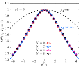
Figure 12: The matrix element ${\cal M}^{B}(z_{1},P_{1}=0)$ (before forming ratios) is shown as a function of quark-antiquark separation $g^{2}z_{1}$ in units of coupling. The different colored symbols are the data taken from $N=0,2,4,8$ flavor theories. The black dashed line is the expectation based on target mass corrections from leading-twist trace terms. The blue dashed line is the behavior modeled by Eq. (52) to take into account the screening behavior of the Wilson-line.

From Fig. 3 in the main text, we can notice that the $P_{1}=0$ matrix element with pion at rest shows a $z_{1}$ dependence. To see why it is interesting, for argument-sake, if we assume that the leading-twist term was the only piece at $P_{1}=0$ OPE, then one simply does not expect any $z_{1}$ dependence. In Fig. 12, we have put together the $P_{1}=0$ data (shown as the points) for ${\cal M}^{B}$ at all flavors $N$ as a function of lattice separation, $z_{1}/a$. For the data shown, the Wilson-line entering the bilocal operator was smeared using 2-steps of Stout. It is quite surprising that the $P_{1}=0$ matrix element shows absolutely no dependence on the flavor or changing $F_{\pi}$ equivalently. Due to the finite valence pion mass, there can be $z_{1}$ dependence from the target mass corrections (TMC) that arises due to trace terms at leading twist Chen et al. (2016b); Radyushkin (2017b). We expect this to be described by

$${\cal M}^{\rm TMC}(z_{1})=1-\frac{(M_{\pi}^{\rm val}z_{1})^{2}}{8}\langle x^{2}\rangle_{v}+{\cal O}\left((M^{\rm val}_{\pi}z_{1})^{4}\right).$$ (51)

To see if this arises because of the TMC, we have plotted Eq. (51) as the dashed black curve, using the value of $\langle x^{2}\rangle\approx 0.2$ that we observed in Fig. 9. This behavior is definitely not sufficient to describe the data. The other $z_{1}$ dependence should, of course, be from the Wilson-line due to its $\exp(-c^{\prime}g^{2}z)$ behavior for larger $|z_{1}|$ with some $c^{\prime}$. Since it should be even with respect to $z_{1}\to-z_{1}$, we model this behavior as

$${\cal M}^{\rm TMC,WL}(z_{1})\equiv\frac{{\cal M}^{\rm TMC}(z_{1})}{\cosh(c^{\prime}g^{2}z_{1})}.$$ (52)

In Fig. 12, we plot ${\cal M}^{\rm TMC,WL}$ as the blue dashed curve using $c^{\prime}=0.281$. The value of $c^{\prime}$ will be dependent on the construction of Wilson-line itself, such as the steps of smearing (in our case, the value of $c^{\prime}$ decreases to 0.206 when 6-step stout was used). We see that ${\cal M}^{\rm TMC,WL}$ nicely describes the data at all $z_{1}$ and for all $N$. Thus, through this exercise, we first understand that the non-perturbative screening behavior of Wilson-line is important in ${\cal M}^{B}$, and therefore, it is very important to form ratios, like in 3+1 dimensions, to get rid of this trivial $z_{1}$ dependence. In Fig. 6, we showed how this cancellation works well by using Wilson-lines with two-different smearing parameters, thereby justifying the application of leading twist framework to the ratio $\tilde{\cal M}$. Secondly, due to universal behavior of ${\cal M}^{B}(P_{1}=0)$ at all $N$, the screening behavior does not care about the infrared physics at all, pointing to the fact that it arises due to the Wilson-line self-interaction at ultraviolet scales.

References

- Dissertori et al. (2003) G. Dissertori, I. G. Knowles, and M. Schmelling, Quantum chromodynamics: high energy experiments and theory, Vol. 115 (Oxford University Press, 2003).
- Liu (2017) C. Liu, PoS LATTICE2016, 006 (2017), arXiv:1612.00103 [hep-lat] .
- Padmanath (2018) M. Padmanath, PoS LATTICE2018, 013 (2018), arXiv:1905.09651 [hep-lat] .
- Briceno et al. (2018) R. A. Briceno, J. J. Dudek, and R. D. Young, Rev. Mod. Phys. 90, 025001 (2018), arXiv:1706.06223 [hep-lat] .
- Accardi et al. (2016) A. Accardi et al., Eur. Phys. J. A 52, 268 (2016), arXiv:1212.1701 [nucl-ex] .
- Ji (1995) X.-D. Ji, Phys. Rev. Lett. 74, 1071 (1995), arXiv:hep-ph/9410274 .
- Hatta and Zhao (2020) Y. Hatta and Y. Zhao, Phys. Rev. D 102, 034004 (2020), arXiv:2006.02798 [hep-ph] .
- Alexandrou et al. (2017) C. Alexandrou, M. Constantinou, K. Hadjiyiannakou, K. Jansen, C. Kallidonis, G. Koutsou, A. Vaquero Avilés-Casco, and C. Wiese, Phys. Rev. Lett. 119, 142002 (2017), arXiv:1706.02973 [hep-lat] .
- Alexandrou et al. (2020) C. Alexandrou, S. Bacchio, M. Constantinou, J. Finkenrath, K. Hadjiyiannakou, K. Jansen, G. Koutsou, H. Panagopoulos, and G. Spanoudes, Phys. Rev. D 101, 094513 (2020), arXiv:2003.08486 [hep-lat] .
- Badier et al. (1983) J. Badier et al. (NA3), Z. Phys. C 18, 281 (1983).
- Betev et al. (1985) B. Betev et al. (NA10), Z. Phys. C 28, 9 (1985).
- Conway et al. (1989) J. Conway et al., Phys. Rev. D 39, 92 (1989).
- Owens (1984) J. Owens, Phys. Rev. D 30, 943 (1984).
- Sutton et al. (1992) P. Sutton, A. D. Martin, R. Roberts, and W. Stirling, Phys. Rev. D 45, 2349 (1992).
- Gluck et al. (1992) M. Gluck, E. Reya, and A. Vogt, Z. Phys. C 53, 651 (1992).
- Gluck et al. (1999) M. Gluck, E. Reya, and I. Schienbein, Eur. Phys. J. C 10, 313 (1999), arXiv:hep-ph/9903288 .
- Wijesooriya et al. (2005) K. Wijesooriya, P. Reimer, and R. Holt, Phys. Rev. C 72, 065203 (2005), arXiv:nucl-ex/0509012 .
- Aicher et al. (2010) M. Aicher, A. Schafer, and W. Vogelsang, Phys. Rev. Lett. 105, 252003 (2010), arXiv:1009.2481 [hep-ph] .
- Brodsky and Farrar (1973) S. J. Brodsky and G. R. Farrar, Phys. Rev. Lett. 31, 1153 (1973).
- Nguyen et al. (2011) T. Nguyen, A. Bashir, C. D. Roberts, and P. C. Tandy, Phys. Rev. C 83, 062201 (2011), arXiv:1102.2448 [nucl-th] .
- Chen et al. (2016a) C. Chen, L. Chang, C. D. Roberts, S. Wan, and H.-S. Zong, Phys. Rev. D 93, 074021 (2016a), arXiv:1602.01502 [nucl-th] .
- Cui et al. (2020) Z.-F. Cui, M. Ding, F. Gao, K. Raya, D. Binosi, L. Chang, C. D. Roberts, J. Rodríguez-Quintero, and S. M. Schmidt, Eur. Phys. J. C 80, 1064 (2020).
- Roberts and Schmidt (2020) C. D. Roberts and S. M. Schmidt (2020) arXiv:2006.08782 [hep-ph] .
- de Teramond et al. (2018) G. F. de Teramond, T. Liu, R. S. Sufian, H. G. Dosch, S. J. Brodsky, and A. Deur (HLFHS), Phys. Rev. Lett. 120, 182001 (2018), arXiv:1801.09154 [hep-ph] .
- Ruiz Arriola (2002) E. Ruiz Arriola, Acta Phys. Polon. B 33, 4443 (2002), arXiv:hep-ph/0210007 .
- Broniowski and Ruiz Arriola (2017) W. Broniowski and E. Ruiz Arriola, Phys. Lett. B 773, 385 (2017), arXiv:1707.09588 [hep-ph] .
- Lan et al. (2020) J. Lan, C. Mondal, S. Jia, X. Zhao, and J. P. Vary, Phys. Rev. D 101, 034024 (2020), arXiv:1907.01509 [nucl-th] .
- Barry et al. (2018) P. Barry, N. Sato, W. Melnitchouk, and C.-R. Ji, Phys. Rev. Lett. 121, 152001 (2018), arXiv:1804.01965 [hep-ph] .
- Novikov et al. (2020) I. Novikov et al., Phys. Rev. D 102, 014040 (2020), arXiv:2002.02902 [hep-ph] .
- Bednar et al. (2020) K. D. Bednar, I. C. Cloët, and P. C. Tandy, Phys. Rev. Lett. 124, 042002 (2020), arXiv:1811.12310 [nucl-th] .
- Ji (2013) X. Ji, Phys. Rev. Lett. 110, 262002 (2013), arXiv:1305.1539 [hep-ph] .
- Ji (2014) X. Ji, Sci. China Phys. Mech. Astron. 57, 1407 (2014), arXiv:1404.6680 [hep-ph] .
- Radyushkin (2017a) A. Radyushkin, Phys. Rev. D 96, 034025 (2017a), arXiv:1705.01488 [hep-ph] .
- Orginos et al. (2017) K. Orginos, A. Radyushkin, J. Karpie, and S. Zafeiropoulos, Phys. Rev. D 96, 094503 (2017), arXiv:1706.05373 [hep-ph] .
- Braun and Müller (2008) V. Braun and D. Müller, Eur. Phys. J. C 55, 349 (2008), arXiv:0709.1348 [hep-ph] .
- Ma and Qiu (2018a) Y.-Q. Ma and J.-W. Qiu, Phys. Rev. D 98, 074021 (2018a), arXiv:1404.6860 [hep-ph] .
- Ma and Qiu (2018b) Y.-Q. Ma and J.-W. Qiu, Phys. Rev. Lett. 120, 022003 (2018b), arXiv:1709.03018 [hep-ph] .
- Constantinou (2020) M. Constantinou, in 38th International Symposium on Lattice Field Theory (2020) arXiv:2010.02445 [hep-lat] .
- Zhao (2019) Y. Zhao, Int. J. Mod. Phys. A 33, 1830033 (2019), arXiv:1812.07192 [hep-ph] .
- Cichy and Constantinou (2019) K. Cichy and M. Constantinou, Adv. High Energy Phys. 2019, 3036904 (2019), arXiv:1811.07248 [hep-lat] .
- Monahan (2018) C. Monahan, PoS LATTICE2018, 018 (2018), arXiv:1811.00678 [hep-lat] .
- Ji et al. (2020) X. Ji, Y.-S. Liu, Y. Liu, J.-H. Zhang, and Y. Zhao, (2020), arXiv:2004.03543 [hep-ph] .
- Gao et al. (2020) X. Gao, L. Jin, C. Kallidonis, N. Karthik, S. Mukherjee, P. Petreczky, C. Shugert, S. Syritsyn, and Y. Zhao, Phys. Rev. D 102, 094513 (2020), arXiv:2007.06590 [hep-lat] .
- Zhang et al. (2019) J.-H. Zhang, J.-W. Chen, L. Jin, H.-W. Lin, A. Schäfer, and Y. Zhao, Phys. Rev. D 100, 034505 (2019), arXiv:1804.01483 [hep-lat] .
- Izubuchi et al. (2019) T. Izubuchi, L. Jin, C. Kallidonis, N. Karthik, S. Mukherjee, P. Petreczky, C. Shugert, and S. Syritsyn, Phys. Rev. D 100, 034516 (2019), arXiv:1905.06349 [hep-lat] .
- Joó et al. (2019) B. Joó, J. Karpie, K. Orginos, A. V. Radyushkin, D. G. Richards, R. S. Sufian, and S. Zafeiropoulos, Phys. Rev. D 100, 114512 (2019), arXiv:1909.08517 [hep-lat] .
- Lin et al. (2020) H.-W. Lin, J.-W. Chen, Z. Fan, J.-H. Zhang, and R. Zhang, (2020), arXiv:2003.14128 [hep-lat] .
- Sufian et al. (2019) R. S. Sufian, J. Karpie, C. Egerer, K. Orginos, J.-W. Qiu, and D. G. Richards, Phys. Rev. D 99, 074507 (2019), arXiv:1901.03921 [hep-lat] .
- Sufian et al. (2020) R. S. Sufian, C. Egerer, J. Karpie, R. G. Edwards, B. Joó, Y.-Q. Ma, K. Orginos, J.-W. Qiu, and D. G. Richards, Phys. Rev. D 102, 054508 (2020), arXiv:2001.04960 [hep-lat] .
- Aguilar et al. (2019) A. C. Aguilar et al., Eur. Phys. J. A 55, 190 (2019), arXiv:1907.08218 [nucl-ex] .
- Adams et al. (2018) B. Adams et al., (2018), arXiv:1808.00848 [hep-ex] .
- Karthik and Narayanan (2018) N. Karthik and R. Narayanan, Phys. Rev. D 97, 054510 (2018), arXiv:1801.02637 [hep-th] .
- Seiberg et al. (2016) N. Seiberg, T. Senthil, C. Wang, and E. Witten, Annals Phys. 374, 395 (2016), arXiv:1606.01989 [hep-th] .
- Karch and Tong (2016) A. Karch and D. Tong, Phys. Rev. X 6, 031043 (2016), arXiv:1606.01893 [hep-th] .
- Choi et al. (2020) C. Choi, D. Delmastro, J. Gomis, and Z. Komargodski, JHEP 03, 078 (2020), arXiv:1810.07720 [hep-th] .
- Sharon (2018) A. Sharon, JHEP 08, 078 (2018), arXiv:1803.06983 [hep-th] .
- Gazit et al. (2018) S. Gazit, F. F. Assaad, S. Sachdev, A. Vishwanath, and C. Wang, Proc. Nat. Acad. Sci. 115, E6987 (2018), arXiv:1804.01095 [cond-mat.str-el] .
- Song et al. (2020) X.-Y. Song, Y.-C. He, A. Vishwanath, and C. Wang, Phys. Rev. X 10, 011033 (2020), arXiv:1811.11182 [cond-mat.str-el] .
- Ma and He (2020) R. Ma and Y.-C. He, Phys. Rev. Res. 2, 033348 (2020), arXiv:2003.05954 [cond-mat.str-el] .
- Chester and Pufu (2016a) S. M. Chester and S. S. Pufu, JHEP 08, 069 (2016a), arXiv:1603.05582 [hep-th] .
- Chester and Pufu (2016b) S. M. Chester and S. S. Pufu, JHEP 08, 019 (2016b), arXiv:1601.03476 [hep-th] .
- Pufu (2014) S. S. Pufu, Phys. Rev. D 89, 065016 (2014), arXiv:1303.6125 [hep-th] .
- Ji et al. (2019) X. Ji, Y. Liu, and I. Zahed, Phys. Rev. D 99, 054008 (2019), arXiv:1807.07528 [hep-ph] .
- Jia et al. (2018) Y. Jia, S. Liang, X. Xiong, and R. Yu, Phys. Rev. D 98, 054011 (2018), arXiv:1804.04644 [hep-th] .
- Del Debbio et al. (2020) L. Del Debbio, T. Giani, and C. J. Monahan, JHEP 09, 021 (2020), arXiv:2007.02131 [hep-lat] .
- Kock et al. (2020) A. Kock, Y. Liu, and I. Zahed, Phys. Rev. D 102, 014039 (2020), arXiv:2004.01595 [hep-ph] .
- Magnea (2000) U. Magnea, Phys. Rev. D 61, 056005 (2000), arXiv:hep-th/9907096 .
- Pisarski (1984) R. D. Pisarski, Phys. Rev. D 29, 2423 (1984).
- Vafa and Witten (1984) C. Vafa and E. Witten, Commun. Math. Phys. 95, 257 (1984).
- Appelquist and Nash (1990) T. Appelquist and D. Nash, Phys. Rev. Lett. 64, 721 (1990).
- Goldman and Mulligan (2016) H. Goldman and M. Mulligan, Phys. Rev. D 94, 065031 (2016), arXiv:1606.07067 [hep-th] .
- Niemi and Semenoff (1983) A. Niemi and G. Semenoff, Phys. Rev. Lett. 51, 2077 (1983).
- Redlich (1984) A. Redlich, Phys. Rev. D 29, 2366 (1984).
- Thomson and Sachdev (2017) A. Thomson and S. Sachdev, Phys. Rev. B 95, 205128 (2017), arXiv:1607.05279 [cond-mat.str-el] .
- Del Debbio and Zwicky (2010) L. Del Debbio and R. Zwicky, Phys. Rev. D 82, 014502 (2010), arXiv:1005.2371 [hep-ph] .
- Rummukainen and Gottlieb (1995) K. Rummukainen and S. A. Gottlieb, Nucl. Phys. B 450, 397 (1995), arXiv:hep-lat/9503028 .
- Braun et al. (1995) V. Braun, P. Gornicki, and L. Mankiewicz, Phys. Rev. D 51, 6036 (1995), arXiv:hep-ph/9410318 .
- Carlson and Freid (2017) C. E. Carlson and M. Freid, Phys. Rev. D 95, 094504 (2017), arXiv:1702.05775 [hep-ph] .
- Briceño et al. (2017) R. A. Briceño, M. T. Hansen, and C. J. Monahan, Phys. Rev. D 96, 014502 (2017), arXiv:1703.06072 [hep-lat] .
- Martinelli and Sachrajda (1987) G. Martinelli and C. T. Sachrajda, Phys. Lett. B 196, 184 (1987).
- Izubuchi et al. (2018) T. Izubuchi, X. Ji, L. Jin, I. W. Stewart, and Y. Zhao, Phys. Rev. D 98, 056004 (2018), arXiv:1801.03917 [hep-ph] .
- Chen et al. (2016b) J.-W. Chen, S. D. Cohen, X. Ji, H.-W. Lin, and J.-H. Zhang, Nucl. Phys. B 911, 246 (2016b), arXiv:1603.06664 [hep-ph] .
- Radyushkin (2017b) A. Radyushkin, Phys. Lett. B 770, 514 (2017b), arXiv:1702.01726 [hep-ph] .
- Dotsenko and Vergeles (1980) V. Dotsenko and S. Vergeles, Nucl. Phys. B 169, 527 (1980).
- Ishikawa et al. (2017) T. Ishikawa, Y.-Q. Ma, J.-W. Qiu, and S. Yoshida, Phys. Rev. D 96, 094019 (2017), arXiv:1707.03107 [hep-ph] .
- Ji et al. (2018) X. Ji, J.-H. Zhang, and Y. Zhao, Phys. Rev. Lett. 120, 112001 (2018), arXiv:1706.08962 [hep-ph] .
- Teper (1999) M. J. Teper, Phys. Rev. D 59, 014512 (1999), arXiv:hep-lat/9804008 .
- Karthik and Narayanan (2016a) N. Karthik and R. Narayanan, Phys. Rev. D 93, 045020 (2016a), arXiv:1512.02993 [hep-lat] .
- Karthik and Narayanan (2015) N. Karthik and R. Narayanan, Phys. Rev. D 92, 025003 (2015), arXiv:1505.01051 [hep-th] .
- Morningstar and Peardon (2004) C. Morningstar and M. J. Peardon, Phys. Rev. D 69, 054501 (2004), arXiv:hep-lat/0311018 .
- Capitani et al. (2006) S. Capitani, S. Durr, and C. Hoelbling, JHEP 11, 028 (2006), arXiv:hep-lat/0607006 .
- Gupta and Karthik (2013) S. Gupta and N. Karthik, Phys. Rev. D 87, 094001 (2013), arXiv:1302.4917 [hep-lat] .
- Duane et al. (1987) S. Duane, A. Kennedy, B. Pendleton, and D. Roweth, Phys. Lett. B 195, 216 (1987).
- Omelyan et al. (2002) I. P. Omelyan, I. M. Mryglod, and R. Folk, Phys. Rev. E 65, 056706 (2002).
- Karthik (2014) N. Karthik, (2014), arXiv:1401.1072 [hep-lat] .
- Gusken et al. (1989) S. Gusken, U. Low, K. Mutter, R. Sommer, A. Patel, and K. Schilling, Phys. Lett. B 227, 266 (1989).
- Bali et al. (2016) G. S. Bali, B. Lang, B. U. Musch, and A. Schäfer, Phys. Rev. D 93, 094515 (2016), arXiv:1602.05525 [hep-lat] .
- Karthik and Narayanan (2016b) N. Karthik and R. Narayanan, Phys. Rev. D 94, 065026 (2016b), arXiv:1606.04109 [hep-th] .
- Mastropas and Richards (2014) E. V. Mastropas and D. G. Richards (Hadron Spectrum), Phys. Rev. D 90, 014511 (2014), arXiv:1403.5575 [hep-lat] .
- Verbaarschot and Zahed (1994) J. Verbaarschot and I. Zahed, Phys. Rev. Lett. 73, 2288 (1994), arXiv:hep-th/9405005 .
- Karpie et al. (2018) J. Karpie, K. Orginos, and S. Zafeiropoulos, JHEP 11, 178 (2018), arXiv:1807.10933 [hep-lat] .
- Appelquist et al. (2020) T. Appelquist et al. (Lattice Strong Dynamics), (2020), arXiv:2007.01810 [hep-ph] .
- Braun et al. (2020) V. Braun, Y. Ji, and A. Manashov, (2020), arXiv:2011.04533 [hep-ph] .