Probing the spin structure of the fractional quantum Hall magnetoroton with polarized Raman scattering

Abstract

Starting from the Luttinger model for the band structure of GaAs, we derive an effective theory that describes the coupling of the fractional quantum Hall (FQH) system with photons in resonant Raman scattering experiments. Our theory is applicable in the regime when the energy of the photons $\omega_{0}$ is close to the energy gap $E_{G}$, but $|\omega_{0}-E_{G}|$ is much larger than the energy scales of the quantum Hall problem. In the literature, it is often assumed that Raman scattering measures the dynamic structure factor $S(\omega,\mathbf{k})$ of the FQH. However, in this paper, we find that the light scattering spectrum measured in the experiments are proportional to the spectral densities of a pair of operators which we identified with the spin-2 components of the kinetic part of the stress tensor. In contrast with the dynamic structure factor, these spectral densities do not vanish in the long-wavelength limit $k\to 0$. We show that Raman scattering with circularly polarized light can measure the spin of the magnetoroton excitation in the FQH system. We give an explicit expression for the kinetic stress tensor that works on any Landau level and which can be used for numerical calculations of the spectral densities that enter the Raman scattering amplitudes. We propose that Raman scattering provides a way to probe the bulk of the $\nu=5/2$ quantum Hall state to determine its nature.

I Introduction

The fractional quantum Hall effect (FQHE) was discovered in experiment almost forty years ago [1]. Fractional quantum Hall (FQH) systems support a host of intriguing physical phenomenons; they are also a playground for many exotic theoretical ideas ranging from anyons [2, 3, 4] to superconductivity [5], skyrmion [6], and bimetric gravity [7], to name a few. Anyonic excitations in a nonabelian FQH states such as the Moore-Read state at filling fraction 5/2 [8] may provide the building blocks for a topological quantum computer [9]. However, FQHE is still one of the most difficult and important unsolved problems of modern physics.

In a classic paper [10], Girvin, MacDonald, and Platzman proposed a single mode approximation for the FQHE, in which the only excitation of the FQH system is a gapped charge-neutral mode called “magnetoroton.” In the original treatment, the magnetoroton was interpreted as the charge density wave in the lowest Landau level (LLL). The dispersion relation of this neutral mode has a minimum at the wave length is of order the magnetic length $\ell_{B}$, which imitate the behavior of the roton mode in superfluid ⁴He. Experiments have confirmed the existence of the magnetoroton mode in light scattering experiments [11, 12, 13] . In the widely accepted theoretical interpretation of these experiments, the light scattering intensity has been associated with the dynamical structure factor $S(\omega,\mathbf{k})$ in the LLL [15]. However, in the LLL limit, the dynamical structure factor goes to zero as $k^{4}$ [10] in the limit where the momentum of the magnetoroton $k$ goes to zero. On the other hand, the Raman signal seems to persist down to $k=0$, signaling that the identification of the intenstity of Raman scattering with the dynamic structure factor may not be correct.

In this paper, we provide a new theoretical treatment for Raman scattering experiments. We first note that the problem of Raman scattering involves many energy scales. The largest energy scale is that of the semiconductor gap $E_{G}$ and the photon energy $\omega_{0}$. The next scale is the distance between the Landau levels of the conduction-band electrons, $\omega_{c}=eB/m^{*}c$, and the smallest energy scale is the Coulomb interacting energy between these electrons, $\Delta$. We assume a hierarchy

$$\Delta\ll\omega_{c}\ll E_{G}.$$ (1)

Only the physics at the scale $\Delta$ is “hard,” i.e., nonperturbative or strongly correlated, while the physics at the scales $E_{G}$ and and $\omega_{c}$ are weakly coupled. To solve the Raman scattering problem effectively, one needs to separate out the nonperturbative, strongly correlated physics at the scale $\Delta$ from the perturbative, weak coupling physics at the other scales. (This is similar to the philosophy of “factorization” in quantum chromodynamics [16] where the perturbative physics at the hadronic scale is separated from the perturbative physics of higher energy scales.)

We perform this “factorization” procedure in two steps. The first is to integrate out the energy scale $E_{G}$. Starting with the Luttinger’s Hamiltonian for GaAs [17], we introduce a coupling between the lowest conduction band and highest valence band due to the interaction with light waves. We focus on the regime of resonant Raman scattering in which the frequency of the incoming light is close to the semiconductor energy gap: $\omega_{0}\approx E_{G}$. Under the assumption that the detuning between the frequency of light and the gap, $|\omega_{0}-E_{G}|$, is larger than both energy scales of the Hall effect $\omega_{c}$ and $\Delta$, we integrate out valence bands to obtain the coupling of the conduction-band electon to the photon. The second step is to do projection to a single Landau level. The result is an effective coupling of the Raman photons to operators acting on a single Landau level.

Our result differs drastically from that of Ref. [15]. We find that instead of measuring the spectral density of the density operator (the dynamic structure factor), the Raman scattering experiment measures the spectral densities of the operators that can be called the “kinetic stress tensor” operators, $T^{\text{kin}}_{ij}=\frac{1}{m^{*}}\partial_{i}\psi^{\dagger}\partial_{j}\psi$. These operatores are the components of the stress tensor that arise from the kinetic energy term in the many-body Hamiltonian. For simple model Hamiltonians leading to exact zero-energy trial wave functions, the kinetic stress tensor coincides with the full stress tensor, but that is not the case for the general case, including that of Coulomb interaction. Moreover, in the lowest Landau level limit, in the long-wavelength limit the only components of the kinetic stress tensor that have nonvanishing spectral densities are the two spin-2 components, $T^{\text{kin}}_{zz}$ and $T^{\text{kin}}_{\bar{z}\bar{z}}$ (the spin-0 component, $T^{\text{kin}}_{z\bar{z}}$ has vanishing spectral density in the limit $k\to 0$).

Recent theoretical works [18, 19, 20, 21] advance a new proposal on the interpretation of the magnetoroton. According to this proposal, the magnetoroton is the quantum a dynamical metric, and at the long-wavelength regime $k\sim 0$ has an angular momentum equals 2 in the direction of the applied magnetic field [19]. In order to determine the spin of the magnetoroton, it has been suggested [19, 20, 21] that the spin of the magnetoroton can be detected through polarized Raman scattering.

We show it this paper how Raman scattering with cicrularly polarized light can indeed be used to confirm the spin of the magnetoroton, including the sign. The basic idea is very simple: if angular momentum is exactly conserved, an FQH state can absorb only one specific circular polarized photon to excite a spin-2 magnetoroton mode and emit a photon with opposite circular polarization. However, the real system does not have full rotational symmetry, but only $C_{4}$, so spins 2 and $-2$ are not distinct from the point of view of symmetry. In this paper we carefully analyze the resonant Raman scattering using the Luttinger model of GaAs. We determine the magnitude of the effect of nonconservation of angular momentum through the Luttinger parameters and show that it is numerically small (of order $1/40$).

We organize the paper as follows. We start Section II by introducing our theoretical model for Raman scattering of an FQH state. In Section III, we present the calculation of the intensity of cirularly polarized light scattering . We show that, in contrast with previous theoretical proposals, the peaks in scattering intensity, at the long wavelength regime, was obtained mainly due to the poles in the correlation functions of the kinetic part of stress tensor $\langle T^{\text{kin}}T^{\text{kin}}\rangle$. We relate the cross section of Raman scattering by circularly polarized light with the spectral densities of the stress tensor. In Section IV, we derive the explicit formulas for the stress tensor projected to a Landau level, which can be used to evaluate numerically the spectral function. We then conclude the paper in Section V. The Appendicies are devoted to the details of the calculation.

II Model

In GaAs the light hole and heavy hole bands make the main contribution to Raman scattering process [15]. Thus the spin-off bands can be ignored in this sense. We consider the effective Lagrangian, with only conduction band $\psi^{\alpha}$ and $j=3/2$ valence bands (which is nothing but light hole and heavy hole bands) $\chi_{i}^{\alpha}$. In the notation, $\alpha=1,2$ represents spinor index, and $i=1,2,3$ represents 3 components of $p$ wave function. The (“Rarita-Schwinger”) constraint is imposed,

$${(\sigma^{i})^{\alpha}}_{\beta}\chi^{\beta}_{i}=0,$$ (2)

which projects out the $j=1/2$ part from $\chi^{\alpha}_{i}$. Consider the Luttinger Hamiltonian for heavy hole and light hole (within approximation $\mathbf{k}\approx 0$) [17]

$$H=\frac{1}{m}\biggl{\{}\left(\gamma_{1}+\frac{5\gamma_{2}}{2}\right)\frac{\mathbf{D}^{2}}{2}-\gamma_{2}\sum_{i}J_{i}^{2}D_{i}^{2}\\ -2\gamma_{3}\left[\{J_{x}J_{y}\}\{D_{x}D_{y}\}+\{J_{y}J_{z}\}\{D_{y}D_{z}\}+\{J_{z}J_{x}\}\{D_{z}D_{x}\}\right]+\frac{e}{c}\kappa\mathbf{J}\cdot\mathbf{B}\biggr{\}},$$ (3)

where $\gamma_{1,2,3}$ are the Luttinger’s parameters, $m$ is the mass of electron, $J_{i}$ are the SO(3) generators: $(J_{i})_{jk}=-i\epsilon_{ijk}$, $D_{i}\chi=(\partial_{i}-i\frac{e}{c}A_{i})\chi$ is the covariant derivative, $\{\cdot\}$ denotes symmetrization, e.g., $\{D_{x}D_{y}\}\equiv\frac{1}{2}(D_{x}D_{y}+D_{y}D_{x})$, and $e<0$ is the electric charge of the electron. Using the equality

$$\{J_{i}J_{j}\}\{D_{i}D_{j}\}=(\mathbf{J}\cdot\mathbf{D})^{2}-\frac{e}{2c}\mathbf{J}\cdot\mathbf{B},$$ (4)

we can rewrite Hamiltonian (3) as

$$H=\frac{1}{m}\biggl{[}\Bigl{(}\gamma_{1}+\frac{5\gamma_{2}}{2}\Bigr{)}\frac{\mathbf{D}^{2}}{2}+(\gamma_{3}-\gamma_{2})\sum_{i}J_{i}^{2}D_{i}^{2}-\gamma_{3}(\mathbf{J}\cdot\mathbf{D})^{2}+\frac{e}{c}\left(\kappa+\frac{\gamma_{3}}{2}\right)\mathbf{J}\cdot\mathbf{B}\biggr{]}.$$ (5)

The Lagrangian for the hole band is

$$\mathcal{L}_{v}=i\chi^{\dagger}_{i\alpha}\partial_{t}\chi^{\alpha}_{i}-\chi^{\dagger}_{i\lambda}H_{ij}\chi^{\lambda}_{j}+E_{G}\chi^{\dagger}_{i\alpha}\chi^{\alpha}_{i},$$ (6)

where $E_{G}$ is energy gap and the covariant derivative is $D_{i}\psi\equiv(\partial_{i}-i\frac{e}{c}A_{i})\psi$. We also have Lagrangian of the conduction band

$$\mathcal{L}_{c}=i\psi_{\alpha}^{\dagger}\partial_{t}\psi^{\alpha}-\frac{D_{i}\psi_{\alpha}^{\dagger}D_{i}\psi^{\alpha}}{2m^{*}}\,,$$ (7)

and the coupling of the valence band and conduction band through interaction with light

$$\mathcal{L}_{i}=e(P^{*}\psi_{\alpha}^{\dagger}\chi^{\alpha}_{i}E_{i}+P\chi^{\dagger}_{i\alpha}\psi^{\alpha}E_{i}),$$ (8)

where $P$ is the strength of the dipole transition between the conduction and valence bands (it will be related to the parameter usually denoted as $E_{p}$ in the literature), $E_{i}$ is the electric field of electromagnetic wave.

We consider the regime of resonant Raman scattering, where the photon energy be is close to the gap: $|\omega_{0}-E_{G}|\ll E_{G}$. Here we chose $\omega_{0}=\frac{\omega_{L}+\omega_{S}}{2}$, with $\omega_{L}$ ($\omega_{S}$) is the frequency of the incoming (scattered) photon. In this case we can write

$$E_{i} =\tilde{E}_{i}e^{-i\omega_{0}t}+\tilde{E}_{i}^{*}e^{i\omega_{0}t},$$ (9)

$$\chi_{i}^{\alpha} =\tilde{\chi}_{i}^{\alpha}e^{i\omega_{0}t},$$ (10)

where $\tilde{E}_{i}$ and $\tilde{\chi}$ are slowly varying fields (e.g., fields that vary with frequencies much smaller than $\omega_{0}$). Subsituting into the action and dropping the rapidly oscillating terms, the action can be rewritten as (for notational simplicity we also drop the tildas in $\tilde{E}_{i}$ and $\tilde{\chi}$)

$$\mathcal{L}=i\psi_{\alpha}^{\dagger}\partial_{t}\psi^{\alpha}-\frac{D_{i}\psi_{\alpha}^{\dagger}D_{i}\psi^{\alpha}}{2m^{*}}+e(P^{*}\psi_{\alpha}^{\dagger}\chi^{\alpha}_{i}E_{i}+P\chi^{\dagger}_{i\alpha}\psi^{\alpha}E_{i}^{*})+i\chi^{\dagger}_{i\alpha}\partial_{t}\chi^{\alpha}_{i}+(E_{G}-\omega_{0})\chi^{\dagger}_{i\alpha}\chi^{\alpha}_{i}\\ -\chi^{\dagger}_{i\lambda}H_{ij}\chi^{\lambda}_{j}+\lambda^{\dagger}_{\alpha}{(\sigma^{i})^{\alpha}}_{\beta}\chi^{\beta}_{i}+\chi^{\dagger}_{i\alpha}{(\sigma^{i})^{\alpha}}_{\beta}\lambda^{\beta}.$$ (11)

The last two terms are Lagrange multiplier for constraints (2).

Integrating out $\chi$ and $\lambda$ is equivalent to solving the field equations and the constraints

$$eP\psi^{\alpha}E_{i}^{*}+(E_{G}-\omega)\chi_{i}^{\alpha}+{(\sigma^{i})^{\alpha}}_{\beta}\lambda^{\beta}+i\partial_{t}\chi_{i}^{\alpha}-H_{ij}\chi^{\alpha}_{j}=0,$$ (12)

$${(\sigma^{i})^{\alpha}}_{\beta}\chi_{i}^{\beta}=0.$$ (13)

We will focus on the regime where the photon energy is not too close to the gap. More precisely, we will assume that the detuning $|\omega_{0}-E_{G}|$ is still much larger than the distance between the Landau levels in the bands,

$$\omega_{c}\equiv\frac{|e|B}{mc}\ll|\omega_{0}-E_{G}|\ll\omega_{0}.$$ (14)

In the FQH regime that and holes the typical momentum scale is $1/\ell_{B}$, one has

$$H\sim\frac{1}{m}D^{2}\sim\frac{eB}{mc}\,.$$ (15)

This means that one can solve Eq. (12), ignoring the $\partial_{t}$ and $H$ terms,

$$\chi^{\alpha}_{i}=-\frac{eP}{3(E_{G}-\omega_{0})}\left[2\psi^{\alpha}E^{*}_{i}+i\epsilon^{ijk}{(\sigma^{j})^{\alpha}}_{\beta}\psi^{\beta}E_{k}^{*}\right]+O\left(\frac{\omega_{c}}{|E_{G}-\omega_{0}|}\right).$$ (16)

Substituting this solution into the action, we then find the effective action for $\psi$ alone. In fact since $\chi$ is the saddlie point, an error of order $O(\omega_{c}/|E_{G}-\omega_{0}|)$ translated into an error $O(\omega_{c}^{2}/|E_{G}-\omega_{0}|^{2})$ in the action; thus it is justified to also keep terms the terms $\chi^{\dagger}\partial_{t}\chi$ and $\chi^{\dagger}H\chi$ when we do the subsitution (16).

To simplify the result, we assume that the electrons are fully polarized with spin $s_{z}=\frac{1}{2}$, so

$$\psi^{\alpha}=\begin{pmatrix}\psi\\ 0\end{pmatrix}.$$ (17)

We assume the incoming and outgoing photons to have momenta along the $z$ direction, so $E_{i}$ are independent of $x$ and $y$. In this case, the Lagrangian describing the interaction of the conduction-band electron with the Raman photons have the form

$$\mathcal{I}_{\text{int}}=V_{\alpha\beta}(E^{*})^{\alpha}E^{\beta},$$ (18)

where $V_{\alpha\beta}$ is some operators quadratic over $\psi$.

The photon spin then points along or opposite to the $z$-axis, corresponding to the two circular polarizations. We will distinguish processes in which the direction of the spin of the photon flips from those in which the photon spin does not change direction. Introducing the complex coordinates (in the quantum Hall convention)

$$z=x-iy,\quad\bar{z}=x+iy,\quad\partial_{z}=\frac{1}{2}(\partial_{x}+i\partial_{y}),\quad\partial_{\bar{z}}=\frac{1}{2}(\partial_{x}-i\partial_{y}),$$ (19)

so

$$E^{z}=E_{x}-iE_{y},\qquad E^{\bar{z}}=E_{x}+iE_{y},$$ (20)

and

$$D_{z}=\frac{1}{2}(D_{x}+iD_{y}),\qquad D_{\bar{z}}=\frac{1}{2}(D_{x}-iD_{y}),$$ (21)

the interaction Lagrangian can be written as

$$\mathcal{I}_{\rm int}=V_{zz}(E^{\bar{z}})^{*}E^{z}+V_{\bar{z}\bar{z}}(E^{z})^{*}E^{\bar{z}}+V_{z\bar{z}}(E^{\bar{z}})^{*}E^{\bar{z}}+V_{\bar{z}z}(E^{z})^{*}E^{z}.$$ (22)

The terms responsible for scatterings with a switch in the photon helicity contain $V_{zz}$ and $V_{\bar{z}\bar{z}}$. Direct calculation yields

$$V_{\bar{z}\bar{z}} =\frac{e^{2}|P|^{2}}{6(E_{G}-\omega_{0})^{2}}\left[(\gamma_{3}+\gamma_{2})D_{z}\psi^{\dagger}D_{z}\psi-(\gamma_{3}-\gamma_{2})D_{\bar{z}}\psi^{\dagger}D_{\bar{z}}\psi\right],$$ (23)

$$V_{zz} =\frac{e^{2}|P|^{2}}{6(E_{G}-\omega_{0})^{2}}\left[(\gamma_{3}+\gamma_{2})D_{\bar{z}}\psi^{\dagger}D_{\bar{z}}\psi-(\gamma_{3}-\gamma_{2})D_{z}\psi^{\dagger}D_{z}\psi\right].$$ (24)

Terms proportional to $\gamma_{3}+\gamma_{2}$ in $V_{zz}$ and $V_{\bar{z}\bar{z}}$ preserves rotational symmetry, while terms proportional to $\gamma_{3}-\gamma_{2}$ breaks the angular momentum conservation by 4.

It is convenient to introduce the “kinetic” stress tensor

$$T_{zz}^{\text{kin}}=\frac{1}{m^{*}}D_{z}\psi^{\dagger}D_{z}\psi,\quad T_{\bar{z}\bar{z}}^{\text{kin}}=\frac{1}{m^{*}}D_{\bar{z}}\psi^{\dagger}D_{\bar{z}}\psi,\quad T_{z\bar{z}}^{\text{kin}}=\frac{1}{2m^{*}}(D_{z}\psi^{\dagger}D_{\bar{z}}\psi+D_{\bar{z}}\psi^{\dagger}D_{z}\psi).$$ (25)

These components are the variation of the kinetic-energy part of the Hamiltonian over the external metric. This is different from the full stress tensor which contains also the variation of the potential energy over the metric. The effective operators coupled to the Raman photon (and flips the direction of its spin) are

$$V_{\bar{z}\bar{z}} =\frac{e^{2}|P|^{2}m^{*}}{6(E_{G}-\omega_{0})^{2}}\left[(\gamma_{3}+\gamma_{2})T_{zz}-(\gamma_{3}-\gamma_{2})T_{\bar{z}\bar{z}}\right],$$ (26)

$$V_{zz} =\frac{e^{2}|P|^{2}m^{*}}{6(E_{G}-\omega_{0})^{2}}\left[(\gamma_{3}+\gamma_{2})T_{\bar{z}\bar{z}}-(\gamma_{3}-\gamma_{2})T_{zz}\right].$$ (27)

For details of calculations see the Appendix A. For completeness, we also write down the operators that do not flip the photon spin,

$$V_{\bar{z}z} =\frac{e^{2}|P|^{2}}{(E_{G}{-}\omega_{0})^{2}}\left[\left(\theta^{*}\omega_{c}{-}\frac{(E_{G}{-}\omega_{0})}{2}{+}\frac{\beta^{*}\omega_{c}}{4}\right)\rho+\left(2\alpha^{*}{-}\beta^{*}{+}\gamma^{\prime*}\right)T_{z\bar{z}}+\frac{i}{2}\psi^{\dagger}\partial_{t}\psi\right],$$ (28a)

$$V_{z\bar{z}} =\frac{e^{2}|P|^{2}}{9(E_{G}{-}\omega_{0})^{2}}\left[\left(-\theta^{*}\omega_{c}{-}\frac{9(E_{G}{-}\omega_{0})}{2}{-}\frac{\beta^{*}\omega_{c}}{4}\right)\rho+\left(6\alpha^{*}{-}5\beta^{*}{+}5\gamma^{\prime*}\right)T_{z\bar{z}}+\frac{9i}{2}\psi^{\dagger}\partial_{t}\psi\right],$$ (28b)

where

$$\alpha^{*} =\frac{m^{*}}{2m}\left(\gamma_{1}+\frac{5\gamma_{2}}{2}\right),\quad\gamma^{\prime*}=\frac{m^{*}}{m}(\gamma_{3}-\gamma_{2}),$$ (29)

$$\beta^{*} =\frac{m^{*}}{m}\gamma_{3},\quad\theta^{*}=-\frac{m^{*}}{m}\left(\kappa+\frac{\gamma_{3}}{2}\right).$$ (30)

III Scattering of circularly polarized light in the FQH regime

In this Section, we will calculate the Raman scattering on the fractional quantum Hall state. The magnitude of the effect can be characterized by the per-particle differential cross-ssection

$$\frac{d\sigma_{\lambda\lambda^{\prime}}}{d\omega d\Omega}\,,$$ (31)

where $\omega$ is the difference between the energy of the incoming photon $\omega_{L}$ and the scattered photon $\omega_{S}$: $\omega=\omega_{L}-\omega_{S}$, $d\Omega$ is the infinitesimal solid angle of the scattered photon, and $\lambda$ and $\lambda^{\prime}$ are the indices denoting the polarization of the incoming and scattered photons. For simplicity, we consider the case when the incident and reflection light are directed perpendicularly to the sample. The light can pass through the sample, or, as depicted in Fig. 1, be reflected from the sample. We will assume that both incident light and scattered lights have circular polarization, and and $\lambda$ and $\lambda^{\prime}$ can be either $+$ and $-$ depending on the projection of the proton spin on the $z$ axis. For example, for $\sigma_{++}$ the incident light is left-handed (in the “classical optics” convention, see, e.g., Ref. [22]) and so the incident photons have spin pointing along the direction of their momentum, and the scattered light is right-handed, as in Fig. 1 (a)),

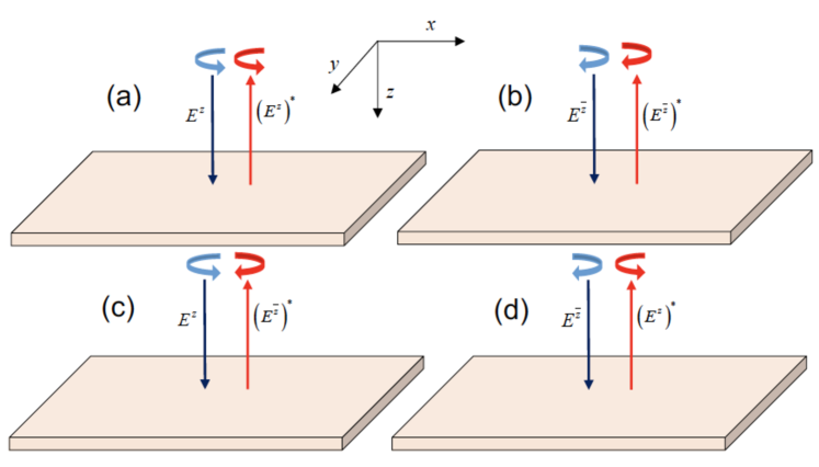
Figure 1: Setup experiment for circular polarized light scattering

we have the formula for cross section per electron [15, 23],

$$\frac{d\sigma_{++}(\omega)}{d\omega d\Omega}=\frac{1}{N_{e}}\frac{\omega_{S}}{\omega_{L}}\omega_{S}^{2}\omega_{L}^{2}\sum_{f}|\langle f|V_{\bar{z}z}|i\rangle|^{2}\delta(\epsilon_{f}-\epsilon_{i}-\hbar\omega)\approx-\frac{1}{\bar{\rho}}\frac{\omega_{0}^{4}}{\pi}\mathop{\mathrm{Im}}\langle V^{\dagger}_{\bar{z}z}V_{\bar{z}z}\rangle_{\omega,\mathbf{0}},$$ (32)

with $N_{e}$ being the total electron number in the conductance band and $\bar{\rho}$ is the electron density in the conductance band, $\epsilon_{f},\epsilon_{i}$ are energies of final and initial states, and

$$\langle A^{\dagger}A\rangle_{\omega,\mathbf{k}}\equiv\int\!dt\,d\mathbf{x}\,e^{i\omega t-i\mathbf{k}\cdot\mathbf{x}}\langle TA(t,\mathbf{x})A^{\dagger}(0,\mathbf{0})\rangle.$$ (33)

Thus we need to calculate the spectral density of the operator $V_{\bar{z}z}(\omega,0)$.

Similarly, in the case of setups in Figure 1 (b), (c), and (d), we have

$$\frac{d\sigma_{--}(\omega)}{d\omega d\Omega} =-\frac{1}{\bar{\rho}}\frac{\omega_{0}^{4}}{\pi}\mathop{\mathrm{Im}}\langle V^{\dagger}_{z\bar{z}}V_{z\bar{z}}\rangle,$$ (34)

$$\frac{d\sigma_{+-}(\omega)}{d\omega d\Omega} =-\frac{1}{\bar{\rho}}\frac{\omega_{0}^{4}}{\pi}\mathop{\mathrm{Im}}\langle V^{\dagger}_{zz}V_{zz}\rangle,$$ (35)

$$\frac{d\sigma_{-+}(\omega)}{d\omega d\Omega} =-\frac{1}{\bar{\rho}}\frac{\omega_{0}^{4}}{\pi}\mathop{\mathrm{Im}}\langle V^{\dagger}_{\bar{z}\bar{z}}V_{\bar{z}\bar{z}}\rangle.$$ (36)

The intensity of the Raman scattering in these channels are proportional to the spectral densities of he operators $V_{z\bar{z}}$, $V_{zz}$, and $V_{\bar{z}\bar{z}}$.

Let us now show that in the limit of negligible Landau level mixing, the spectral densities of the operators $V_{z\bar{z}}$ and $V_{\bar{z}z}$ are zero, implying that the processes depicted on Fig. 1 (a) and (b) do not happen. For that, we note from Eqs. (28) that the integrals of $V_{z\bar{z}}$ and $V_{\bar{z}z}$ over space are linear combinations of

$$\int\!d\mathbf{x}\,\rho,\quad\int\!d\mathbf{x}\,T_{z\bar{z}}^{\text{kin}},\quad\int\!d\mathbf{x}\,i\psi^{\dagger}\partial_{t}\psi.$$ (37)

The first integral is the total number of particles $N_{e}$. As this quantity is conserved, it does not contribute to the spectral density. From Appendix D we find the results for $N^{th}$ Landau level

$$\int\!d\mathbf{x}\,T_{z\bar{z}}^{\text{kin}} =(N+\frac{1}{2})\frac{\omega_{c}}{2}N_{e},$$ (38)

$$\int\!d\mathbf{x}\,i\psi^{\dagger}\partial_{t}\psi =2E-(N+\frac{1}{2})\omega_{c}N_{e},$$ (39)

where $E$ is the total energy. Both integrals reduce to conserved quantities. Thus, the Raman processes that does not involve flipping the direction of the photon spin are suppressed.

In previous experiments [11, 12], the momentum transfer to the electron gass is rather small $kl_{B}\leq 0.15$. This implies that these experiments mainly probe the transitions where the photon spin flips sign, and effectively measures the spectral densities of the traceless components of the kinetic stress tensor. The picture suggested here is different from the previous one suggested in Ref. [15] where the main coupling of the Raman photon to the electron liquids is through the $\psi^{\dagger}\psi A_{i}^{2}$ term in the Lagrangian. This coupling would lead to a vanishing Raman scattering at $k=0$.

Let us introduce the short-hand notation for the spectral densities of the off-diagonal components of the stress tensor,

$$-\mathop{\mathrm{Im}}\left\langle T_{zz}^{\text{kin}}T_{\bar{z}\bar{z}}^{\text{kin}}\right\rangle_{\omega,\mathbf{0}} =I_{+}(\omega),$$ (40)

$$-\mathop{\mathrm{Im}}\left\langle T_{\bar{z}\bar{z}}^{\text{kin}}T_{zz}^{\text{kin}}\right\rangle_{\omega,\mathbf{0}} =I_{-}(\omega).$$ (41)

These functions should be calculated numerically. The intensity of Raman scatterings can now be expressed as

$$\frac{d\sigma_{+-}}{d\omega d\Omega}= \frac{1}{\pi\bar{\rho}}\left[\frac{e^{2}|P|^{2}\omega_{0}^{2}m^{*}}{6(E_{0}-\omega_{0})^{2}}\right]^{2}\left[(\gamma_{3}+\gamma_{2})^{2}I_{+}(\omega)+(\gamma_{3}-\gamma_{2})^{2}I_{-}(\omega)\right],$$ (42)

$$\frac{d\sigma_{-+}}{d\omega d\Omega}= \frac{1}{\pi\bar{\rho}}\left[\frac{e^{2}|P|^{2}\omega_{0}^{2}m^{*}}{6(E_{0}-\omega_{0})^{2}}\right]^{2}\left[(\gamma_{3}+\gamma_{2})^{2}I_{-}(\omega)+(\gamma_{3}-\gamma_{2})^{2}I_{+}(\omega)\right].$$ (43)

In Ref. [24] it was proven that $I_{+}(\omega)=0$ for the trial ground states of model Hamiltonians with contact interactions. While there is no argument that $I_{+}$ should be zero for more general Hamiltonians, numerically it was found that for Coulomb interaction $I_{+}$ is much smaller than $I_{-}$ for the Laughlin $\nu=1/3$ state [20].

If one ignore $I_{+}$ compared to $I_{-}$, we find the ratio of scattered light intensity of experiment setups 1 (c) and 1 (d)

$$\frac{I_{-+}(\omega=\Delta)}{I_{+-}(\omega=\Delta)}=\frac{(\gamma_{3}+\gamma_{2})^{2}}{(\gamma_{3}-\gamma_{2})^{2}}\,.$$ (44)

The ratio only depends on the Luttinger parameters. Moreover, the fact that $I_{+-}$ will vanish if $\gamma_{3}-\gamma_{2}=0$ suggests that the signal of $I_{+-}$ is due to rotational symmetry breaking. These results confirm that at zero momentum ($\mathbf{k}=0$), the magneto-roton excitation has spin 2 in $\hat{z}$ direction. However, in the case of finite momentum, the magneto-roton excitation will be mixed of modes with spin $+2$ and spin $-2$ in $\hat{z}$ direction, which was suggested in the previous work [19].

The numerical values for the Luttinger parameters of GaAs are [25]

$$\gamma_{1}=6.9,\quad\gamma_{2}=2.1,\quad\gamma_{3}=2.9,\quad\kappa=1.2.$$ (45)

Substituting these parameters in equation (44) yields the ratio of intensities

$$\frac{I_{-+}(\omega=\Delta)}{I_{+-}(\omega=\Delta)}\approx 40.$$ (46)

Note that this relies on the assumption that $I_{+}=0$, which is not expected to hold exactly for the Coulomb interaction. However, if $I_{+}$ is small compared to $I_{-}$, one still expect that $I_{-+}\ll I_{+-}$ for $\nu=1/3$ states. This is also expected for the Jain states $\nu=n/(2n+1)$, in which the composite fermion theory implies that the magnetoroton has the same sign of spin as in the $\nu=1/3$ state. In the particle-hole conjugate Jain states $\nu=(n+1)/(2n+1)$, in contrast, one expects that $I_{-+}\gg I_{+-}$ [26, 27].

IV Stress tensor projected on a Landau level

As we have seen from the previous section, to obtain the cross section of polarized Raman scattering, we need to calculate the spectral function of the kinetic part of the stress tensor projected on a specific Landau level (the fractionally filled one). To enable future numerical calculations of these spectral functions we need the expressions for the operators $T^{\text{kin}}_{ij}$ after the projection to a Landau level. In this section, we will derive the explicit form of the projected kinetic stress tensor.

We summarize the result here. For a system of particles interacting through a two-body isotropic potential $V(|\mathbf{x}-\mathbf{y}|)$ on the $N$th Landau level, the kinetic part of the stress tensor (at zero momentum) can be written as

$$\int\!d\mathbf{x}\,T_{ij}^{\text{kin}}=\int_{\mathbf{q}}\frac{q_{i}q_{j}}{q}\frac{\partial}{\partial q}\left\{e^{-x_{q}}[L_{N}(x_{q})]^{2}\right\}V(q)\bar{\rho}(\mathbf{q})\bar{\rho}(-\mathbf{q}),$$ (47)

where $\int_{\mathbf{q}}\equiv\int\!d\mathbf{q}/(2\pi)^{2}$,

$$x_{q}\equiv\frac{q^{2}\ell_{B}^{2}}{2}\,,$$ (48)

$L_{N}(x)$ is the Laguerre polynomial, and $ij$ can be either $zz$ or $\bar{z}\bar{z}$, and $\bar{\rho}(\mathbf{q})$ is the projected density operator in momentum space [10].

The interpretation of the above equation is rather simple. Recall that the projected Hamiltonian of the system is

$$H=\int_{\mathbf{q}}e^{-x_{q}}[L_{N}(x_{q})]^{2}V(q)\bar{\rho}(\mathbf{q})\bar{\rho}(-\mathbf{q}),$$ (49)

where the form-factor $e^{-x_{q}}[L_{N}(x_{q})]^{2}$ arises from the projection to the $N$th Landau level. Polarized Raman scattering, as explained above, has the effect of changing the effective metric in the kinetic term for the electron (making the effective mass $m^{*}$ anisotropic). This makes the Landau orbit on the $N$th Landau level anistropic, and the effect of that is the operator $(q_{i}q_{j}/q)\partial_{q}$ acting on the form-factor.

For $N=0$, Eq. (47) reads

$$\int\!d\mathbf{x}\,T_{zz}^{\text{kin}}=-\ell_{B}^{2}\int_{\mathbf{q}}q_{z}^{2}e^{-q^{2}\ell_{B}^{2}/2}V(q)\bar{\rho}(\mathbf{q})\bar{\rho}(-\mathbf{q}),$$ (50)

which is exactly the operator considered in Ref. [20]. Thus the spectral densities computed in Ref. [20] are directly related to polarized Raman scattering on FQH states on the LLL.

For the next-to-lowest Landau level $N=1$ we have

$$\int\!d\mathbf{x}\,T_{zz}^{\text{kin}}=-\ell_{B}^{2}\int_{\mathbf{q}}q_{z}^{2}e^{-x_{q}}(1-x_{q})(3-x_{q})V(q)\bar{\rho}(\mathbf{q})\bar{\rho}(-\mathbf{q}).$$ (51)

The general expression for the kinetic stress tensor (47) has also been found by Kun Yang [28]. In the rest of this Section, we provide a derivation of Eq. (47).

IV.1 Preliminaries

We use the complex coordinates (19) and the symmetric gauge $A_{x}=-\frac{1}{2}By$, $A_{y}=\frac{1}{2}Bx$. In the complex coordinates

$$A_{z}=\frac{1}{2}(A_{x}+iA_{y})=i\frac{B}{4}\bar{z},\qquad A_{\bar{z}}=\frac{1}{2}(A_{x}-iA_{y})=-i\frac{B}{4}z,$$ (52)

Then in the symmetric gauge

$$D_{z} =\partial_{z}-\frac{ie}{c}A_{z}=\partial_{z}-\frac{\bar{z}}{4}\,,$$ (53)

$$D_{\bar{z}} =\partial_{\bar{z}}-\frac{ie}{c}A_{\bar{z}}=\partial_{\bar{z}}+\frac{z}{4}\,.$$ (54)

Note that

$$[D_{z},\,D_{\bar{z}}]=-\frac{eB}{2c}=\frac{1}{2\ell_{B}^{2}}\,.$$ (55)

The (complex) guiding center coordinates are defined as

$$Z =z-2\ell_{B}^{2}D_{\bar{z}}=\frac{z}{2}-2\ell_{B}^{2}\partial_{\bar{z}},$$ (56)

$$\bar{Z} =\bar{z}+2\ell_{B}^{2}D_{z}=\frac{\bar{z}}{2}+2\ell_{B}^{2}\partial_{z}$$ (57)

which satisfy

$$[D_{z},\,Z]=[D_{z},\,\bar{Z}]=[D_{\bar{z}},\,Z]=[D_{\bar{z}},\,\bar{Z}]=0.$$ (58)

and

$$[\bar{Z},\,Z]=2\ell_{B}^{2}.$$ (59)

We define another set of coordinates: the relative coordinates which describes the motion around the guiding center,

$$\zeta =2\ell_{B}^{2}D_{\bar{z}}=\frac{z}{2}+2\ell_{B}^{2}\partial_{\bar{z}},$$ (60)

$$\bar{\zeta} =-2\ell_{B}^{2}D_{z}=\frac{\bar{z}}{2}-2\ell_{B}^{2}\partial_{z},$$ (61)

which commute with $Z$ and $\bar{Z}$ [Eqs. (58)] and have the commutator

$$[\bar{\zeta},\,\zeta]=-2\ell_{B}^{2}.$$ (62)

Then $z=Z+\zeta$, $\bar{z}=\bar{Z}+\bar{\zeta}$. We denote the 2D vector whose complex coordinates are $Z$ and $\bar{Z}$ as $\mathbf{R}$, and the vector with complex coordinates $\zeta$ and $\bar{\zeta}$ as $\tilde{\mathbf{r}}$. That means $\mathbf{x}=\mathbf{R}+\tilde{\mathbf{r}}$.

One defines two sets of creation and annihilation operators. One set moves between different Landau levels

$$a=\sqrt{2}\ell_{B}D_{\bar{z}}=\frac{\zeta}{\sqrt{2}\ell_{B}},\qquad a^{\dagger}=-\sqrt{2}\ell_{B}D_{z}=\frac{\bar{\zeta}}{\sqrt{2}\ell_{B}}\,,$$ (63)

and another set moves within a Landau level

$$b=\frac{1}{\sqrt{2}\ell_{B}}\bar{Z},\qquad b^{\dagger}=\frac{1}{\sqrt{2}\ell_{B}}Z.$$ (64)

The orbitals are obtained by acting creation operator on the lowest state

$$|M,m\rangle=\frac{1}{\sqrt{M!m!}}a^{\dagger M}b^{\dagger m}|0,0\rangle,$$ (65)

where

$$\langle\mathbf{x}|0,0\rangle\sim e^{-|z|^{2}/4\ell_{B}^{2}}.$$ (66)

IV.2 The kinetic stress tensor on a Landau level

Our task is to find the expression for the kinetic part of the stress tensor in the theory where the electrons live on one Landau level. This will be done through a field-theory formalism. The action describing electrons on the $N$th Landau level is

$$S=\int\!dt\,d\mathbf{x}\left[i\psi^{\dagger}\partial_{t}\psi+\chi^{\dagger}\left(2\ell_{B}^{2}D_{z}D_{\bar{z}}\psi+N\psi\right)+\left(2\ell_{B}^{2}D_{\bar{z}}D_{z}\psi^{\dagger}+N\psi^{\dagger}\right)\chi\right]\\ -\frac{1}{2}\!\int\!dt\,d\mathbf{x}\,d\mathbf{x}^{\prime}\,V(\mathbf{x}-\mathbf{x}^{\prime})\psi^{\dagger}(\mathbf{x})\psi^{\dagger}(\mathbf{x}^{\prime})\psi(\mathbf{x}^{\prime})\psi(\mathbf{x}).$$ (67)

The fields $\chi$ and $\chi^{\dagger}$ are simply the Lagrange multipliers enforcing the constraint

$$2\ell_{B}^{2}D_{z}D_{\bar{z}}\psi+N\psi=0,$$ (68)

which is simply the condition that $\psi$ lies on the $N$th Landau level.

To find the stress tensor, we first rewrite the action by integration by part,

$$S=\int\!dt\,d\mathbf{x}\left[i\psi^{\dagger}\partial_{t}\psi-2\ell_{B}^{2}D_{z}\chi^{\dagger}D_{\bar{z}}\psi-2\ell_{B}^{2}D_{z}\psi^{\dagger}D_{\bar{z}}\chi+N(\chi^{\dagger}\psi+\psi^{\dagger}\chi)\right]\\ -\frac{1}{2}\!\int\!dt\,d\mathbf{x}\,d\mathbf{x}^{\prime}\,V(\mathbf{x}-\mathbf{x}^{\prime})\psi^{\dagger}(\mathbf{x})\psi^{\dagger}(\mathbf{x}^{\prime})\psi(\mathbf{x}^{\prime})\psi(\mathbf{x}),$$ (69)

then the kinetic part of the stress tensor can be calculated from Noether’s theorem:

$${T^{i}}_{j}=-\frac{\partial L}{\partial(\partial_{i}\phi_{a})}\partial_{j}\phi_{a},$$ (70)

where one sums over all fields $\phi_{a}$, which in our case encompass $\psi$, $\phi^{\dagger}$, $\chi$, and $\chi^{\dagger}$. For the polarized Raman experiment with perpendicularly incoming and outgoing photons, with a flipping of the photon spin, one only needs the traceless part of the stress tensor, integrated over space:

$$\int\!d\mathbf{x}\,T^{\text{kin}}_{zz} =-\ell_{B}^{2}\int\!d\mathbf{x}\,(\chi^{\dagger}D_{z}^{2}\psi+D_{z}^{2}\psi^{\dagger}\chi),$$ (71)

$$\int\!d\mathbf{x}\,T^{\text{kin}}_{\bar{z}\bar{z}} =-\ell_{B}^{2}\int\!d\mathbf{x}\,(\chi^{\dagger}D_{\bar{z}}^{2}\psi+D_{\bar{z}}^{2}\psi^{\dagger}\chi).$$ (72)

We can expand $\chi$ as a sum over Landau levels: $\chi=\chi_{0}+\chi_{1}+\chi_{2}+\cdots$. We recall that when acting on $\psi$ and $\chi$, $D_{z}$ raises and $D_{\bar{z}}$ lowers the Landau level index, while when acting on $\psi^{\dagger}$ and $\chi^{\dagger}$ they switch roles. Due to the orthogonality of wavefunctions on different Landau levels, only the parts of $\chi$ that are on the $(N+2)$th and (if $N\geq 2$) $(N-2)$th Landau level’s contribute to the integrals in Eqs. (71). We then have, for $N\geq 2$

$$\int\!d\mathbf{x}\,T^{\text{kin}}_{zz} =-\ell_{B}^{2}\int\!d\mathbf{x}\,(\chi_{N+2}^{\dagger}D_{z}^{2}\psi+D_{z}^{2}\psi^{\dagger}\chi_{N-2}),$$ (73)

$$\int\!d\mathbf{x}\,T^{\text{kin}}_{\bar{z}\bar{z}} =-\ell_{B}^{2}\int\!d\mathbf{x}\,(\chi_{N-2}^{\dagger}D_{\bar{z}}^{2}\psi+D_{\bar{z}}^{2}\psi^{\dagger}\chi_{N+2}),$$ (74)

and for $N=0$ or 1

$$\int\!d\mathbf{x}\,T^{\text{kin}}_{zz} =-\ell_{B}^{2}\int\!d\mathbf{x}\,\chi_{N+2}^{\dagger}D_{z}^{2}\psi,$$ (75)

$$\int\!d\mathbf{x}\,T^{\text{kin}}_{\bar{z}\bar{z}} =-\ell_{B}^{2}\int\!d\mathbf{x}\,D_{\bar{z}}^{2}\psi^{\dagger}\chi_{N+2}.$$ (76)

The equation determining $\chi$ is

$$0=\frac{\delta S}{\delta\psi^{\dagger}}=i\partial_{t}\psi+(2\ell_{B}^{2}D_{z}D_{\bar{z}}+N)\chi+W(\mathbf{x}),$$ (77)

which, for $n\neq N$, implies

$$\chi_{n}=\frac{W_{n}}{n-N}\,.$$ (78)

In particular

$$\chi_{N+2} =\frac{1}{2}W_{N+2}\,,$$ (79)

$$\chi_{N-2} =-\frac{1}{2}W_{N-2}\,\quad(N\geq 2),$$ (80)

and therefore

$$\int\!d\mathbf{x}\,T^{\text{kin}}_{zz} =-\frac{1}{2}\ell_{B}^{2}\int\!d\mathbf{x}\,(W^{\dagger}D_{z}^{2}\psi-D_{z}^{2}\psi^{\dagger}W),$$ (81)

$$\int\!d\mathbf{x}\,T^{\text{kin}}_{\bar{z}\bar{z}} =\frac{1}{2}\ell_{B}^{2}\int\!d\mathbf{x}\,(W^{\dagger}D_{\bar{z}}^{2}\psi-D_{\bar{z}}^{2}\psi^{\dagger}W),$$ (82)

where we have used the orthogonality of the functions on different Landau levels to replace $W_{N+2}$ and $W_{N-2}$ by simply $W$.

Using formulas of Appendix C, we then find

$$\int\!d\mathbf{x}\,T^{\text{kin}}_{zz}=-\frac{1}{2}\int_{\mathbf{q}}\ell_{B}^{2}q_{z}^{2}e^{-x_{q}}L_{N}(x_{q})\left[L_{N}^{2}(x_{q})-L_{N-2}^{2}(x_{q})\right]V(q)\bar{\rho}(\mathbf{q})\bar{\rho}(-\mathbf{q}),\quad x_{q}\equiv\frac{q^{2}\ell_{B}^{2}}{2}\,,$$ (83)

and a similar equation where $T_{zz}$ is replaced by $T_{\bar{z}\bar{z}}$ and $q_{z}$ by $q_{\bar{z}}$. Here $L_{N}$ is the Laguerre polynomial and $L_{N}^{2}$ is not the square of $L_{N}$ but the associate Laguerre polynomial $L_{N}^{k}$ with $k=2$, and for the uniformity of the equation we have defined $L^{2}_{-1}=L^{2}_{-2}=0$.

These equations can be brought to an alternative form by using the following identities involving the associated Laguerre polynomials,

$$L_{N}^{k}(x)=L_{N}^{k+1}(x)-L_{N-1}^{k+1}(x),\qquad\frac{d}{dx}L^{k}_{N}(x)=-L_{N-1}^{k+1}(x).$$ (84)

One can show that, for $N\geq 2$

$$L_{N}^{2}(x)-L_{N-2}^{2}(x)=L_{N}(x)-2\frac{d}{dx}L_{N}(x),$$ (85)

while one can also check directly that

$$L_{0}(x)\left[L_{0}(x)-2L^{\prime}_{0}(x)\right]=L_{0}(x)L_{0}^{2}(x),\qquad L_{1}(x)\left[L_{1}(x)-2L^{\prime}_{1}(x)\right]=L_{1}(x)L_{1}^{2}(x).$$ (86)

We then can rewrite the kinetic part of stress tensor for a general Landau level $N$ as

$$\int\!d\mathbf{x}\,T^{\rm kin}_{zz}=-\frac{\ell_{B}^{2}}{2}\sum_{\mathbf{q}}q_{z}^{2}e^{-x_{q}}L_{N}(x_{q})\left[L_{N}(x_{q})-2L^{\prime}_{N}(x_{q})\right]V(q)\bar{\rho}(\mathbf{q})\bar{\rho}(-\mathbf{q}),$$ (87)

and another equation with the replacement $T_{zz}^{\text{kin}}\to T_{\bar{z}\bar{z}}^{\text{kin}}$ and $q_{z}\to q_{\bar{z}}$. This can be further transformed to Eq. (47).

Some remarks are in order. The kinetic part of stress tensor operators (87) for the LLL share the same form as the spin-2 operators in Ref [20], in which the authors calculated the normalized spectral functions. One can employ the same approach to obtain the spectral density of the stress tensor for higher Landau levels. The result will provide the estimation for Raman scattering intensity of an FQH system at higher Landau levels in our theoretical model. In Appendix E, we give the expression for the full stress tensor operators, including the contribution from the interaction. This can be used calculate the spectral function of LLL stress tensor and check the sum rules derived in Ref. [19].

V Conclusions

In this paper, we have derived the coupling of the electrons in a single Landau level with applied electromagnetic waves, which effectively captures the essential physics of Raman scattering on FQH systems. We show that the electron operator responsible for Raman scattering is not the density operator, but the “kinetic stress tensor,” and we derive the expression of the latter after projection to a single Landau level. We then show that, in the long-wavelength regime, the light scattering intensity in Raman experiments measures the spectral function of the kinetic part of stress tensors. Our calculation explains the scattering intensity peaks at zero momentum without relying on any momentum-noncoserving processes.

In addition, we proposed experimental setups to verify the spin-2 hypothesis of magneto-roton mode in FQH systems using Raman scattering with circularly polarized light. We show that, for a magnetoroton with a well-defined sign of spin, the ratio between light scattering intensities of different configurations of circularly polarized Raman experiments only depends on Luttinger parameters, which are well known. Measuring those ratios can confirm our theoretical model and unveil the spin of the magnetoroton excitations in a FQH state.

Using the explicit form of the stress tensor operator derived in this paper, one can perform the numerical calculation to obtain the stress tensors’ spectral function. One then use the numerical results to verify the LLL sum rules proposed in Ref. [19], and to predict the result of Raman scattering on states on higher Landau levels.

Raman scattering may help resolve the question about the nature of the $\nu=5/2$ state. In a recent experiment [29], the thermal Hall conductance at the edge of the $\nu=5/2$ state was determined to be consistent with the PH-Pfaffian state [30], but not the Pfaffian [8], or the anti-Pfaffian state [31, 32], seemingly contradicting the results of numerical simulations [33]. Theoretical proposals aiming to explain this discrepancy include a disorder-stabilized thermal metal phase which is adiabatically connected to the PH-Pfaffian phase [34, 35] and an incomplete thermalization on the edge [36, 37, 38]. Raman scattering provides a way to probe directly the bulk of the $\nu=5/2$ state. The magnetoroton in the Pfaffian (Moore-Read) state [8] must have a spin of the same sign as in the $\nu=1/3$ Lauglin state, while in the anti-Pfaffian state [31, 32] it must have the opposite sign. The PH-Pfaffian state [30], in the absence of Landau-level mixing, is particle-hole symmetric, hence the Raman scattering probabilities $I_{+-}$ and $I_{-+}$ must be the same. However, it is not clear how significant the effect of Landau level mixing would be in this case.

To derive the coupling of the Raman photons to FQH electron liquid, we have assume that the detuning $|\omega_{0}-E_{G}|$ is much larger than the cyclotron energy $\omega_{c}$. This allows us to perform the first step of our “factorization” procedure—integrating out the holes—without having to think about the effect of the magnetic field on the conduction-band electrons. We suspect that our final result is valid under a weaker assumption—that the detuning is larger than the energy scale of the FQHE, i.e., of the Coulomb interaction between the conduction-band electrons. A derivation of this result would need to be a one-step procedure—integrating out the valence bands and the projecting to one Landau level at the same time. We defer this to future work.

Appendix A Detailed derivation of Raman scattering coupling

In this section, we present the detailed derivation the coupling of the FQH system with photon. We define new parameters

$$\alpha =\frac{1}{2m}\left(\gamma_{1}+\frac{5\gamma_{2}}{2}\right),\quad\gamma^{\prime}=\frac{1}{m}(\gamma_{3}-\gamma_{2}),$$ (88)

$$\beta =\frac{1}{m}\gamma_{3},\quad\theta=-\frac{1}{m}\left(\kappa+\frac{\gamma_{3}}{2}\right).$$ (89)

After integrating out fields in valence band, we derive the effective Lagrangian for conduction band

$$\mathcal{L}=i\psi_{\alpha}^{\dagger}\partial_{t}\psi^{\alpha}-\frac{D_{i}\psi_{\alpha}^{\dagger}D_{i}\psi^{\alpha}}{2m^{*}}+i\chi^{\dagger}_{i\alpha}\partial_{t}\chi^{\alpha}_{i}-(E_{G}-\omega_{0})\chi^{\dagger}_{i\alpha}\chi^{\alpha}_{i}\\ -\chi^{\dagger}_{k^{\prime}\lambda}\biggl{[}\alpha\mathbf{D}^{2}+\gamma^{\prime}\sum_{i}J_{i}^{2}D_{i}^{2}-\beta(\mathbf{J}\cdot\mathbf{D})^{2}-\frac{e}{c}\theta\mathbf{J}\cdot\mathbf{B}\biggr{]}_{k^{\prime}k}\chi^{\lambda}_{k}.$$ (90)

All terms which contain valence band field $\chi^{\alpha}_{i}$ can be considered as coupling of conduction band field $\psi^{\alpha}$ with the electric field through substitution (16). We define

$$\mathcal{I}_{0} =i\chi_{i\lambda}^{\dagger}\partial_{t}\chi_{i}^{\lambda},$$ (91)

$$\mathcal{I}_{1} =-(E_{G}-\omega_{0})\chi^{\dagger}_{i\alpha}\chi^{\alpha}_{i},$$ (92)

$$\mathcal{I}_{\alpha} =-\alpha\chi^{\dagger}_{k\lambda}\mathbf{D}^{2}\chi^{\lambda}_{k},$$ (93)

$$\mathcal{I}_{\beta} =\beta\chi^{\dagger}_{k^{\prime}\lambda}\left[(\mathbf{J}\cdot\mathbf{D})^{2}\right]_{k^{\prime}k}\chi^{\lambda}_{k},$$ (94)

$$\mathcal{I}_{\gamma^{\prime}} =-\gamma^{\prime}\chi^{\dagger}_{k^{\prime}\lambda}\sum_{i}(J_{i}^{2})_{k^{\prime}k}D_{i}^{2}\chi^{\lambda}_{k},$$ (95)

$$\mathcal{I}_{\theta} =\theta\frac{e}{c}\sum_{k,k^{\prime},\lambda}\chi^{\dagger}_{k^{\prime}\lambda}(\mathbf{J}_{k^{\prime}k}\cdot\mathbf{B})\chi^{\lambda}_{k}.$$ (96)

Consequently, the effective Lagrangian can be rewritten as

$$\mathcal{L}_{\rm eff}=i\psi^{\dagger}\partial_{t}\psi-\frac{(D_{i}\psi)^{\dagger}D_{i}\psi}{2m^{*}}+\mathcal{I}_{0}+\mathcal{I}_{1}+\mathcal{I}_{\alpha}+\mathcal{I}_{\beta}+\mathcal{I}_{\gamma^{\prime}}+\mathcal{I}_{\theta}.$$ (97)

Substitution of equation (16) for $\chi^{\alpha}_{i}$ in equation (92) yields

$$\mathcal{I}_{1}=-\frac{e^{2}|P|^{2}}{3(E_{G}-\omega_{0})}\left[2\psi^{\dagger}\psi|E|^{2}+i\epsilon^{ijk}\psi^{\dagger}\sigma^{j}\psi E_{k}^{*}E_{i}\right].$$ (98)

The first term in $\mathcal{I}_{1}$ is the interaction of light with charge density, the second term is the interaction of light with spin density. Considering that the electrons in the conduction band, under strong magnetic field in $\hat{z}$ direction, only have the spin component $s_{z}=\frac{1}{2}$, we can rewrite

$$\mathcal{I}_{1}=-\frac{e^{2}|P|^{2}}{3(E_{G}-\omega_{0})}\left[2E_{i}E_{i}^{*}+i(E_{2}^{*}E_{1}-E_{1}^{*}E_{2})\right]\rho,$$ (99)

where $\rho=\psi^{\dagger}\psi$. Since $E_{i}^{*}$ is a slow varying field under the redefinition (9), the term with $\partial_{t}E_{i}^{*}$ in $\mathcal{I}_{0}$ is small in comparison with $\mathcal{I}_{1}$. We then have

$$\mathcal{I}_{0}=i\frac{e^{2}|P|^{2}}{3(E_{G}-\omega_{0})^{2}}\left[2E_{i}E_{i}^{*}+i(E_{2}^{*}E_{1}-E_{1}^{*}E_{2})\right]\psi^{\dagger}\partial_{t}\psi.$$ (100)

To understand the next interaction terms (the Luttinger terms), we recall the formula for the kinetic part of stress energy tensor

$$T^{\rm kin}_{ij}=\frac{(D_{i}\psi)^{\dagger}D_{j}\psi}{2m^{*}}+\frac{(D_{j}\psi)^{\dagger}D_{i}\psi}{2m^{*}}.$$ (101)

Under above assumption of spin state of electrons in the conduction band and $k_{3}=0$ (we consider 2D system in $xy$ plane, and the applied magnetic field is in $\hat{z}$ direction), we can rewrite the Luttinger terms as

$$\mathcal{I}_{\alpha}=\frac{\alpha^{*}e^{2}|P|^{2}}{3(E_{G}-\omega_{0})^{2}}\left[2E_{i}E_{i}^{*}+i(E_{2}^{*}E_{1}-E_{1}^{*}E_{2})\right](T^{\rm kin}_{11}+T^{\rm kin}_{22}),$$ (102)

$$\mathcal{I}_{\beta}= -\frac{\beta^{*}e^{2}|P|^{2}}{9(E_{G}-\omega_{0})^{2}}\left\{T^{\rm kin}_{11}\left[5E_{2}E_{2}^{*}+5E_{3}E_{3}^{*}+2E_{1}E_{1}^{*}+i(E_{2}E_{1}^{*}-E_{1}E_{2}^{*})\right]\right.$$ (103)

$$\left.+T^{\rm kin}_{22}\left[5E_{1}E_{1}^{*}+5E_{3}E_{3}^{*}+2E_{2}E_{2}^{*}+i(E_{2}E_{1}^{*}-E_{1}E_{2}^{*})\right]\right.$$

$$\left.-3T^{\rm kin}_{12}\left(E_{1}E_{2}^{*}+E_{2}E_{1}^{*}\right)+i\frac{\omega_{c}}{2c}\left[5(E_{2}E_{1}^{*}-E_{1}E_{2}^{*})-4iE_{a}E_{a}^{*}-2iE_{3}E_{3}^{*}\right]\rho\right\},$$

$$\mathcal{I}_{\gamma^{\prime}}= \frac{{\gamma^{\prime}}^{*}e^{2}|P|^{2}}{9(E_{G}-\omega_{0})^{2}}\left\{T^{\rm kin}_{11}\left[5E_{2}E_{2}^{*}+5E_{3}E_{3}^{*}+2E_{1}E_{1}^{*}+i(E_{2}E_{1}^{*}-E_{1}E_{2}^{*})\right]\right.$$

$$\left.+T^{\rm kin}_{22}\left[5E_{1}E_{1}^{*}+5E_{3}E_{3}^{*}+2E_{2}E_{2}^{*}+i(E_{2}E_{1}^{*}-E_{1}E_{2}^{*})\right]\right\},$$ (104)

$$\mathcal{I}_{\theta}=i\theta^{*}\omega_{c}\frac{e^{2}|P|^{2}}{9(E_{G}-\omega_{0})^{2}}\left[5(E_{1}E_{2}^{*}-E_{2}E_{1}^{*})+4iE_{a}E_{a}^{*}+2iE_{3}E_{3}^{*}\right]\rho,$$ (105)

where we have defined the parameters

$$\beta^{*}=\beta m^{*},\quad\alpha^{*}=\alpha m^{*},$$ (106)

$$\gamma^{\prime*}=\gamma^{\prime}m^{*},\quad\theta^{*}=\theta m^{*},$$ (107)

and the cyclotron frequency

$$\omega_{c}=-\frac{eB}{cm^{*}}=\frac{|eB|}{cm^{*}}.$$ (108)

The effective Lagrangian for the conduction band includes the coupling of the electric field $E_{i}$ with charge density $\rho$ and the kinetic part of stress energy tensor $T^{\rm kin}_{ij}$. We have the effective interaction of conduction band with light through $\mathcal{I}_{0},\mathcal{I}_{1},\mathcal{I}_{\alpha},\mathcal{I}_{\beta},\mathcal{I}_{\gamma^{\prime}},\mathcal{I}_{\theta}$. We can rewrite the interaction term in the convenient form for circular polarized light scattering experiment setup in the Figure 1. In this case, we can consider $E_{3}=0,E_{3}^{*}=0$. Going to the complex coordinates (19) and (20), in which

$$T^{\rm kin}_{zz}=\frac{1}{4}(T^{\rm kin}_{xx}-T^{\rm kin}_{yy}+2iT^{\rm kin}_{xy}),\quad T^{\rm kin}_{\bar{z}\bar{z}}=\frac{1}{4}(T^{\rm kin}_{xx}-T^{\rm kin}_{yy}-2iT^{\rm kin}_{xy}),\quad T^{\rm kin}_{z\bar{z}}=\frac{1}{4}(T^{\rm kin}_{xx}+T^{\rm kin}_{yy}),$$ (109)

we can rewrite the interaction terms as

$$\mathcal{I}_{0}=i\frac{e^{2}|P|^{2}}{6(E_{G}-\omega_{0})^{2}}\left[3E^{\bar{z}}(E^{\bar{z}})^{*}+E^{z}(E^{z})^{*}\right]\psi^{\dagger}\partial_{t}\psi,$$ (110)

$$\mathcal{I}_{1}=-\frac{e^{2}|P|^{2}}{6(E_{G}-\omega_{0})}\left[3E^{\bar{z}}(E^{\bar{z}})^{*}+E^{z}(E^{z})^{*}\right]\rho,$$ (111)

$$\mathcal{I}_{\alpha}=\alpha^{*}\frac{e^{2}|P|^{2}}{3(E_{G}-\omega_{0})^{2}}\left[6E^{\bar{z}}(E^{\bar{z}})^{*}+2E^{z}(E^{z})^{*}\right]T^{\rm kin}_{z\bar{z}},$$ (112)

$$\mathcal{I}_{\beta}=-\frac{\beta^{*}e^{2}|P|^{2}}{9(E_{G}-\omega_{0})^{2}}\left\{-3E^{z}(E^{\bar{z}})^{*}T^{\rm kin}_{zz}-3E^{\bar{z}}(E^{z})^{*}T^{\rm kin}_{\bar{z}\bar{z}}+(5E^{z}(E^{z})^{*}+9E^{\bar{z}}(E^{\bar{z}})^{*})T^{\rm kin}_{z\bar{z}}\right.\\ \left.+\frac{\omega_{c}}{4}(E^{z}(E^{z})^{*}-9E^{\bar{z}}(E^{\bar{z}})^{*})\rho\right\},$$ (113)

$$\mathcal{I}_{\gamma^{\prime}}= \frac{\gamma^{\prime*}e^{2}|P|^{2}}{9(E_{G}-\omega_{0})^{2}}\left\{-\frac{3}{2}\left[E^{z}(E^{\bar{z}})^{*}+E^{\bar{z}}(E^{z})^{*}\right](T^{\rm kin}_{zz}+T^{\rm kin}_{\bar{z}\bar{z}})+\left[5E^{z}(E^{z})^{*}+9E^{\bar{z}}(E^{\bar{z}})^{*}\right]T^{\rm kin}_{z\bar{z}}\right\},$$ (114)

$$\mathcal{I}_{\theta}=\theta^{*}\frac{\omega_{c}e^{2}|P|^{2}}{18(E_{G}-\omega_{0})^{2}}\left[E^{z}(E^{z})^{*}-9E^{\bar{z}}(E^{\bar{z}})^{*}\right]\rho.$$ (115)

We can easily check that only $\mathcal{I}_{\gamma^{\prime}}$ violates rotational invariance.

Appendix B The dipole-transition oefficient $P$

In this Appendix, we follow Ref. [39] to derive an expression for the dipole-transition coefficient $P$ through the electron Bloch wave functions. The first term of Eq. (8) absorbs a photon and creates a hole in the valence band and adds an electron to the conductance band. We can rewrite this term in the Hamiltonian as

$$-\int\!dx\,eP^{*}_{ij}\psi^{\alpha\dagger}\chi^{i}_{\alpha}E^{j},$$ (116)

with $P_{ij}^{*}=P^{*}\delta_{ij}$. Comparing with Eq. (11.23) in Ref. [39], we see that

$$-eP_{ij}^{*}i\omega_{ph}\left<n_{ph}{-}1|A^{j}|n_{ph}\right>=-\frac{e}{m}\left<\psi^{\alpha}_{\mathbf{k}},n_{ph}{-}1|A^{j}p_{j}|\chi_{i\alpha,\mathbf{k}},n_{ph}\right>,$$ (117)

with $m$ being the free electron mass and $p_{j}$ is the free electron momentum operator. Then we have

$$P^{*}_{ij}=-\frac{i}{m\omega_{ph}}\left<\psi^{\alpha}_{\mathbf{k}}|p_{j}|\chi_{i\alpha,\mathbf{k}}\right>,$$ (118)

where $\psi^{\alpha}_{\mathbf{k}}$ is the Bloch wavefunction of electron in the conductance band ($s$-band)

$$\psi^{\alpha}_{\mathbf{k}}=\frac{1}{\sqrt{N_{\rm site}}}\sum_{a}e^{i\mathbf{k}\cdot\mathbf{x}}u^{\alpha}_{c}(\mathbf{x}-\mathbf{R}_{a}),$$ (119)

and $\chi_{i\alpha,\mathbf{k}}$ is the Bloch wavefunction of electron in the valence bands (p-band)

$$\chi_{i\alpha,\mathbf{k}}=\frac{1}{\sqrt{N_{\rm site}}}\sum_{a}e^{i\mathbf{k}\cdot\mathbf{x}}u^{i\alpha}_{v}(\mathbf{x}-\mathbf{R}_{a}).$$ (120)

We have

$$\left<\psi^{\alpha}_{\mathbf{k}}|p_{j}|\chi_{i\alpha,\mathbf{k}}\right>=\frac{1}{N_{\rm site}}\sum_{a,b}\int\!d^{3}\mathbf{x}\,[k_{j}(u^{\alpha})^{*}_{c}(\mathbf{x}-\mathbf{R}_{a})u^{i\alpha}_{v}(\mathbf{x}-\mathbf{R}_{b})-i(u^{\alpha})^{*}_{c}(\mathbf{x}-\mathbf{R}_{a})\partial_{j}u^{i\alpha}_{v}(\mathbf{x}-\mathbf{R}_{b})],$$ (121)

The first term vanishes due to the orthogonality of LCAO. The second term can be written as

$$\left<\psi^{\alpha}_{\mathbf{k}}|p_{j}|\chi_{i\alpha,\mathbf{k}}\right>=-i\sum_{a,b}\int_{\text{unit cell}}d^{3}\mathbf{x}\,(u^{\alpha})^{*}_{c}(\mathbf{x}-\mathbf{R}_{a})\partial_{j}u^{i\alpha}_{v}(\mathbf{x}-\mathbf{R}_{b}).$$ (122)

Due to the angular momentum conservation, we have

$$\left<\psi^{\alpha}_{\mathbf{k}}|p_{j}|\chi_{i\alpha,\mathbf{k}}\right>=-i\delta_{ij}\sum_{a,b}\int_{\text{unit cell}}d^{3}\mathbf{x}\,(u^{\alpha})^{*}_{c}(\mathbf{x}-\mathbf{R}_{a})\partial_{i}u^{i\alpha}_{v}(\mathbf{x}-\mathbf{R}_{b}).$$ (123)

Following Ref. [39], we obtain

$$\left<\psi^{\alpha}_{\mathbf{k}}|p_{i}|\chi_{i\alpha,\mathbf{k}}\right>=|\hat{e}\cdot\vec{p}_{\rm cv}|,$$ (124)

where $\hat{e}$ is any unit vector and $p^{x}_{\rm cv}=p^{y}_{\rm cv}=p^{z}_{\rm cv}$ with the definition

$$p^{i}_{\rm cv}=-i\sum_{a,b}\int_{\text{unit cell}}d^{3}\mathbf{x}\,(u^{\alpha})^{*}_{c}(\mathbf{x}-\mathbf{R}_{a})\partial_{i}u^{i\alpha}_{v}(\mathbf{x}-\mathbf{R}_{b}).$$ (125)

We also have the relation between $|\hat{e}\cdot\vec{p}_{\rm cv}|$ and the parameter $E_{p}$ often use in the photonics literature [39]

$$|\hat{e}\cdot\vec{p}_{\rm cv}|^{2}=\frac{E_{p}m}{2}\,.$$ (126)

We then obtain

$$P^{*}=-\frac{i}{m\omega_{ph}}\sqrt{\frac{E_{p}m}{2}}\,.$$ (127)

Note that the coupling depends on the frequency of photon. However, if we rewrite the coupling with electric field to coupling with gauge potential, there will be no dependence on the photon frequency. We can rewrite the coupling with photon (8) as

$$\mathcal{L}_{i}=e\sqrt{\frac{E_{p}}{2m}}(\psi_{\alpha}^{\dagger}\chi^{\alpha}_{i}A_{i}+\chi^{\dagger}_{i\alpha}\psi^{\alpha}A_{i}^{*}).$$ (128)

Appendix C How to project to a Landau level

In this section, we provide the detail calculation for kinetic part of stress tensor in a specific Landau level. The electron field can be expanded in orbitals

$$\psi(\mathbf{x})=\sum_{Mm}\langle\mathbf{x}|Mm\rangle c_{Mm},$$ (129)

where $M$ labels the Landau level, and $m$ labels the states within the Landau level. In order to obtain the kinetic part of stress tensor, we need to compute

$$\int\!d\mathbf{x}\,W^{\dagger}(\mathbf{x})D_{z}^{2}\psi(\mathbf{x})=-\!\int\!d\mathbf{x}\,d\mathbf{x}^{\prime}\,\psi^{\dagger}(\mathbf{x})\psi^{\dagger}(\mathbf{x}^{\prime})V(\mathbf{x}-\mathbf{x}^{\prime})\psi(\mathbf{x}^{\prime})D_{z}^{2}\psi(\mathbf{x}).$$ (130)

Inserting the expansion over modes, and limiting to the $N$th Landau level, this becomes

$$-\int\!d\mathbf{x}\,d\mathbf{x}^{\prime}\sum_{mnm^{\prime}n^{\prime}}\langle Nm|\mathbf{x}\rangle\langle Nm^{\prime}|\mathbf{x}^{\prime}\rangle V(\mathbf{x}-\mathbf{x}^{\prime})\langle\mathbf{x}^{\prime}|Nn^{\prime}\rangle D_{z}^{2}\langle\mathbf{x}|Nn\rangle c^{\dagger}_{Nm}c^{\dagger}_{Nm^{\prime}}c_{Nn^{\prime}}c_{Nn}.$$ (131)

Introducing the Fourier transform of the potential

$$V(\mathbf{x}-\mathbf{x}^{\prime})=\int\!\frac{d\mathbf{q}}{(2\pi)^{2}}\,e^{i\mathbf{q}\cdot(\mathbf{x}-\mathbf{x}^{\prime})}V(\mathbf{q}),$$ (132)

the expression becomes

$$-\!\sum_{mnm^{\prime}n^{\prime}}\int_{\mathbf{q}}V(\mathbf{q})\!\int\!d\mathbf{x}\,\langle Nm|\mathbf{x}\rangle e^{i\mathbf{q}\cdot\mathbf{x}}D_{z}^{2}\langle\mathbf{x}|Nn\rangle\!\int\!d\mathbf{x}^{\prime}\,\langle Nm^{\prime}|\mathbf{x}^{\prime}\rangle e^{-i\mathbf{q}\cdot\mathbf{x}^{\prime}}\langle\mathbf{x}^{\prime}|Nn^{\prime}\rangle c^{\dagger}_{m}c^{\dagger}_{m^{\prime}}c_{n^{\prime}}c_{n}.$$ (133)

Now we have

$$\int\!d\mathbf{x}^{\prime}\,\langle Nm^{\prime}|\mathbf{x}^{\prime}\rangle e^{-i\mathbf{q}\cdot\mathbf{x}^{\prime}}\langle\mathbf{x}^{\prime}|Nn^{\prime}\rangle=\langle Nm^{\prime}|e^{-i\mathbf{q}\cdot\hat{\mathbf{x}}}|Nn^{\prime}\rangle=\langle N|e^{-i\mathbf{q}\cdot\tilde{\mathbf{r}}}|N\rangle\langle m^{\prime}|e^{-i\mathbf{q}\cdot\mathbf{R}}|n^{\prime}\rangle,$$ (134)

but

$$\langle N|e^{-i\mathbf{q}\cdot\tilde{\mathbf{r}}}|N\rangle=\langle N|\exp\left[-\frac{i\ell_{B}}{\sqrt{2}}(q^{z}a^{\dagger}+q^{\bar{z}}a)\right]|N\rangle\\ =e^{-x_{q}/2}\langle N|\exp\left(-\frac{i\ell_{B}}{\sqrt{2}}q^{z}a^{\dagger}\right)\exp\left(-\frac{i\ell_{B}}{\sqrt{2}}q^{\bar{z}}a\right)|N\rangle=e^{-x_{q}/2}L_{N}(x_{q}),\quad x_{q}=\frac{q^{2}\ell_{B}^{2}}{2}\,,$$ (135)

therefore

$$\sum_{m^{\prime}n^{\prime}}\!\int\!d\mathbf{x}^{\prime}\,\langle Nm^{\prime}|\mathbf{x}^{\prime}\rangle e^{-i\mathbf{q}\cdot\mathbf{x}^{\prime}}\langle\mathbf{x}^{\prime}|Nn^{\prime}\rangle c^{\dagger}_{m^{\prime}}c_{n^{\prime}}=e^{-x_{q}/2}L_{N}(x_{q})\bar{\rho}(\mathbf{q}).$$ (136)

Analogously

$$\int\!d\mathbf{x}\,\langle Nm|\mathbf{x}\rangle e^{i\mathbf{q}\cdot\mathbf{x}}D_{z}^{2}\langle\mathbf{x}|Nn^{\prime}\rangle=\frac{1}{2}\langle Nm|e^{i\mathbf{q}\cdot\hat{\mathbf{x}}}\frac{a^{\dagger 2}}{\ell_{B}^{2}}|Nn\rangle\\ =\frac{1}{2\ell_{B}^{2}}\sqrt{(N+1)(N+2)}\langle N|e^{i\mathbf{q}\cdot\tilde{\mathbf{r}}}|N+2\rangle\langle m|e^{i\mathbf{q}\cdot\mathbf{R}}|n\rangle=-q_{z}^{2}e^{-x_{q}/2}L_{N}^{2}(x_{q})\langle m|e^{i\mathbf{q}\cdot\mathbf{R}}|n\rangle,$$ (137)

therefore

$$\sum_{mn}\!\int\!d\mathbf{x}\,\langle Nm|\mathbf{x}\rangle e^{-i\mathbf{q}\cdot\mathbf{x}}D_{z}^{2}\langle\mathbf{x}|Nn\rangle c^{\dagger}_{m}c_{n}=-q_{z}^{2}e^{-x_{q}/2}L_{N}^{2}(x_{q})\bar{\rho}(-\mathbf{q}).$$ (138)

Finally we obtain

$$\int\!d\mathbf{x}\,W^{\dagger}(\mathbf{x})D_{z}^{2}\psi(\mathbf{x})=\int\!\frac{d\mathbf{q}}{(2\pi)^{2}}\,q_{z}^{2}e^{-x_{q}}L_{N}(x_{q})L_{N}^{2}(x_{q})V(q)\bar{\rho}(\mathbf{q})\bar{\rho}(-\mathbf{q}).$$ (139)

Similarly, for $N\geq 2$

$$\int\!d\mathbf{x}\,W^{\dagger}(\mathbf{x})D_{\bar{z}}^{2}\psi(\mathbf{x})=\int\!\frac{d\mathbf{q}}{(2\pi)^{2}}\,q_{\bar{z}}^{2}e^{-x_{q}}L_{N}(x_{q})L_{N-2}^{2}(x_{q})V(q)\bar{\rho}(\mathbf{q})\bar{\rho}(-\mathbf{q}),$$ (140)

while for $N=0$ or 1 the expression is obviously zero due to the presence of two lowering operators $D_{\bar{z}}$ acting on $\psi$. Equations (139) and (140) are used in Sec. IV to obtain the explicit form of the kinetic part of stress tensor on a specific Landau level.

Appendix D $i\psi^{\dagger}\partial_{t}\psi$ and $T^{\rm kin}_{z\bar{z}}$

In this Appendix, we derive the explicit form of $i\psi^{\dagger}\partial_{t}\psi$ in the lowest Landau level. The field equation reads

$$i\partial_{t}\psi(\mathbf{x})=-\frac{1}{m^{*}}\left(D_{z}D_{\bar{z}}+D_{\bar{z}}D_{z}\right)\psi(\mathbf{x})+\int\!d\mathbf{x}^{\prime}\,V(\mathbf{x}-\mathbf{x}^{\prime})\psi^{\dagger}(\mathbf{x}^{\prime})\psi(\mathbf{x}^{\prime})\psi(\mathbf{x}),$$ (141)

we then use the constraint equation $2\ell_{B}^{2}D_{z}D_{\bar{z}}\psi=-N\psi$ and the commutator (55) from that we get

$$i\!\int\!d\mathbf{x}\,\psi^{\dagger}\partial_{t}\psi=I_{0}+(N+\frac{1}{2})\omega_{c}N_{e},$$ (142)

with $N_{e}$ being the total electron number in the conductance band and

$$I_{0}=\int\!d\mathbf{x}\,d\mathbf{x}^{\prime}\,V(\mathbf{x}-\mathbf{x}^{\prime})\psi^{\dagger}(\mathbf{x})\psi^{\dagger}(\mathbf{x}^{\prime})\psi(\mathbf{x}^{\prime})\psi(\mathbf{x})=\int_{\mathbf{q}}V(\mathbf{q})e^{-q^{2}\ell_{B}^{2}/2}\bar{\rho}(\mathbf{q})\bar{\rho}(-\mathbf{q}).$$ (143)

The first term on the on the right hand side of Eq. (142) is twice the interacting energy and second term is the kinetic energy of electrons. We also have

$$\int\!d\mathbf{x}\,T^{\rm kin}_{z\bar{z}} =\int\!d\mathbf{x}\,\frac{1}{2m^{*}}\left(D_{z}\psi^{\dagger}D_{\bar{z}}\psi+D_{\bar{z}}\psi^{\dagger}D_{z}\psi\right)$$

$$=\int\!d\mathbf{x}\,\frac{1}{2m^{*}}\left(-2\psi^{\dagger}D_{z}D_{\bar{z}}\psi-\frac{eB}{2c}\psi^{\dagger}\psi\right)$$

$$=\frac{\omega_{c}}{2}(N+\frac{1}{2})\!\int\!d\mathbf{x}\,\rho=(N+\frac{1}{2})\frac{N_{e}\omega_{c}}{2}.$$ (144)

Where we used the contraint $2\ell_{B}^{2}D_{z}D_{\bar{z}}\psi=-N\psi$ to obtain the last equality.

Appendix E Two sum rules

This Appendix is not directly related to Raman scattering, but contains some exact sum rules. First we write down formulas for the full stress tensor. For the model Hamiltonian, at the long wave length regime $\mathbf{k}\sim 0$, the full stress tensor is the same as $T^{\rm kin}$ [24]. For the general case, one needs to take into account the potential-energy term in the Lagrangian. When the metric varies with time (but remains uniform in space), the potential changes according to

$$V(\mathbf{x})\to V(\sqrt{g_{ij}x^{i}x^{j}}),$$ (145)

and so the Fourier transform changes as

$$V(\mathbf{q})\to V(\sqrt{g^{ij}q_{i}q_{j}}).$$ (146)

Given that the stress tensor is give by $\delta S=\frac{1}{2}\int\!dx\,T_{ij}\delta g_{ij}$, the potential part of the stress-energy tensor is then

$$\int\!d\mathbf{x}\,T_{ij}^{\rm pot}=\frac{1}{2}\int_{\mathbf{q}}\frac{q_{i}q_{j}}{q}V^{\prime}(q)\rho(\mathbf{q})\rho(-\mathbf{q}).$$ (147)

This can be projected to the $N$th Landau level to become

$$\int\!d\mathbf{x}\,T_{ij}^{\rm pot}=\frac{1}{2}\int_{\mathbf{q}}e^{-x_{q}}\left[L_{N}(x_{q})\right]^{2}\frac{q_{i}q_{j}}{q}V^{\prime}(q)\bar{\rho}(\mathbf{q})\bar{\rho}(-\mathbf{q}).$$ (148)

It is interesting to compare the formula to to that of the kinetic stress tensor, Eq. (47): the “stretching operator” $(q_{i}q_{j}/q)\partial_{q}$ now acts on the potential $V(q)$ instead of acting on the form-factor. The full stress tensor is the sum of the kinetic stress tensor, Eqs. (87), and the potential stress tensor, Eq. (148). It can be written as

$$\int\!d\mathbf{x}\,T_{ij}^{\text{full}}=\frac{1}{2}\sum_{\mathbf{q}}\frac{q_{i}q_{j}}{q}\frac{\partial}{\partial q}\left\{e^{-x_{q}}[L_{N}(x_{q})]^{2}V(q)\right\}\bar{\rho}(\mathbf{q})\bar{\rho}(-\mathbf{q}).$$ (149)

We define the spectral densities [19]

$$\rho_{T}(\omega) =\frac{1}{N}\sum_{n}|\langle n|\int\!d\mathbf{x}\,T_{zz}|0\rangle|^{2}\delta(\omega-E_{n}),$$ (150)

$$\bar{\rho}_{T}(\omega) =\frac{1}{N}\sum_{n}|\langle n|\int\!d\mathbf{x}\,T_{\bar{z}\bar{z}}|0\rangle|^{2}\delta(\omega-E_{n}),$$ (151)

where $N$ is the total number of electrons, $|0\rangle$ is the ground state, the sum is taken over all excited states $|n\rangle$ in the lowest Landau level, and $E_{n}$ is the energy of the state $|n\rangle$. The two spectrum densities satisfy the sum rules [19]

$$\int_{0}^{\infty}\frac{d\omega}{\omega^{2}}\left[\rho_{T}(\omega)-\bar{\rho}_{T}(\omega)\right] =\frac{\bar{s}}{4}\,,$$ (152)

$$\int_{0}^{\infty}\frac{d\omega}{\omega^{2}}\left[\rho_{T}(\omega)+\bar{\rho}_{T}(\omega)\right] =S_{4},$$ (153)

where $\bar{s}$ is the “guiding center spin” [18], which is equal to $(\mathcal{S}-1)/2$ on the LLL where $\mathcal{S}$ is the shift, and $S_{4}$ is the coefficient in front of $(k\ell_{B})^{4}$ in the static structure factor.