A Julia implementation of Algorithm NCL
for constrained optimization

Abstract

Algorithm NCL is designed for general smooth optimization problems where first and second derivatives are available, including problems whose constraints may not be linearly independent at a solution (i.e., do not satisfy the LICQ). It is equivalent to the LANCELOT augmented Lagrangian method, reformulated as a short sequence of nonlinearly constrained subproblems that can be solved efficiently by IPOPT and KNITRO, with warm starts on each subproblem. We give numerical results from a Julia implementation of Algorithm NCL on tax policy models that do not satisfy the LICQ, and on nonlinear least-squares problems and general problems from the CUTEst test set.

1 Introduction

Algorithm NCL (nonlinearly constrained augmented Lagrangian [15]) is designed for smooth, constrained optimization problems for which first and second derivatives are available. Without loss of generality, we take the problem to be

NCO $${\displaystyle\mathop{\mathrm{minimize}}_{x\in\mathds{R}^{n}}}$$

subject to

where $\phi(x)$ is a scalar objective function and $c(x)\in\mathds{R}^{m}$ is a vector of linear or nonlinear constraints. Inequality constraints are accommodated by including slack variables within $x$. We take the primal and dual solutions to be $(x^{\ast},y^{\ast},z^{\ast})$. We denote the objective gradient by $g(x)=\nabla\phi(x)\in\mathds{R}^{n}$, and the constraint Jacobian by $J(x)\in\mathds{R}^{m\times n}$. The objective and constraint Hessians are $H_{i}(x)\in\mathds{R}^{n\times n}$, $i=0,1,\dots,m$.

If $J(x^{\ast})$ has full row rank $m$, problem NCO satisfies the linear independence constraint qualification (LICQ) at $x^{\ast}$. Most constrained optimization solvers have difficulty if NCO does not satisfy the LICQ. An exception is LANCELOT [4, 5, 13]. Algorithm NCL inherits this desirable property by being equivalent to the LANCELOT algorithm. Assuming first and second derivatives are available, Algorithm NCL may be viewed as an efficient implementation of the LANCELOT algorithm. Previously we have implemented Algorithm NCL in AMPL [1, 6, 15] for tax policy problems [11, 15] that could not otherwise be solved. Here we describe our implementation in Julia [3] and give results on the tax problems and on a set of nonlinear least-squares problems from the CUTEst test set [9].

2 LANCELOT and NCL

For problem NCO, LANCELOT implements what we call a BCL algorithm (bound-constrained augmented Lagrangian algorithm), which solves a sequence of about 10 bound-constrained subproblems

BC_k $${\displaystyle\mathop{\mathrm{minimize}}_{x}}$$

subject to

for $k=0,1,2,\dots$, where $y_{k}$ is an estimate of the dual variable associated with $c(x)=0$, and $\rho_{k}>0$ is a penalty parameter. Each subproblem BC_k is solved (approximately) with a decreasing optimality tolerance $\omega_{k}$, giving an iterate $(x^{*}_{k},z^{*}_{k})$. If $\|c(x^{*}_{k})\|$ is no larger than a decreasing feasibility tolerance $\eta_{k}$, the dual variable is updated to $y_{k+1}=y_{k}-\rho_{k}c(x^{*}_{k})$. Otherwise, the penalty parameter is increased to $\rho_{k+1}>\rho_{k}$.

Optimality is declared if $c(x^{*}_{k})\leq\eta_{k}$ and $\eta_{k}$, $\omega_{k}$ have already been decreased to specified minimum values $\eta^{\ast}$, $\omega^{\ast}$. Infeasibility is declared if $c(x^{*}_{k})>\eta_{k}$ and $\rho_{k}$ has already been increased to a specified maximum value $\rho^{\ast}$.

If $n$ is large and not many bounds are active at $x^{\ast}$, the BC_k subproblems have many degrees of freedom, and LANCELOT must optimize in high-dimension subspaces. The subproblems are therefore computationally expensive. The algorithm in MINOS [16] (we call it an LCL algorithm) reduces this expense by including linearizations of the constraints within its subproblems:

LC_k $${\displaystyle\mathop{\mathrm{minimize}}_{x}}$$

subject to

The SQP algorithm in SNOPT [8] solves subproblems with the same linearized constraints and a quadratic approximation to the LC_k objective. Complications arise for both MINOS and SNOPT if the linearized constraints are infeasible.

Algorithm NCL proceeds in the opposite way by introducing additional variable $r\equiv-c(x)$ into subproblems LC_k to obtain the NCL subproblems

NC_k $${\displaystyle\mathop{\mathrm{minimize}}_{x,\,r}}$$

subject to

These subproblems have nonlinear constraints and far more degrees of freedom than the original NCO! Indeed, the extra variables $r$ make the subproblems more difficult if they are solved by MINOS and SNOPT. However, the subproblems satisfy the LICQ because of $r$. Also, interior solvers such as IPOPT [10] and KNITRO [12] find $r$ helpful because at each interior iteration $p$ they update the current primal-dual point $(x_{p},r_{p},\lambda_{p})$ by computing a search direction $(\Delta x,\Delta r,\Delta\lambda)$ from a linear system of the form

$$\begin{pmatrix}(H_{p}+D_{p})&&J_{p}^{T}\\ &\!\!\!\!\rho_{k}I&I\\ J_{p}&I&\end{pmatrix}\begin{pmatrix}\Delta x\\ \Delta r\\ \Delta\lambda\end{pmatrix}=-\begin{pmatrix}g(x_{p})+J_{p}^{T}\lambda_{p}-z_{p}+w_{p}\\ y_{k}+\rho_{k}r_{p}+\lambda_{p}\\ c(x_{p})+r_{p}\end{pmatrix},$$ (1)

where $D_{p}$, $z_{p}$ and $w_{p}$ are an ill-conditioned positive-definite diagonal matrix and two vectors arising from the interior method, and each Lagrangian Hessian $H_{p}=H_{0}(x_{p})-\sum_{i}(y_{k})_{i}H_{i}(x_{p})$ may be altered to be more positive definite. Direct methods for solving each sparse system (1) are affected very little by the higher dimension caused by $r$, and they benefit significantly from $\begin{pmatrix}J_{p}&I\end{pmatrix}$ always having full row rank.

If an optimal solution for NC_k is $(x^{*}_{k},r^{*}_{k},y^{*}_{k},z^{*}_{k})$ and the feasibility and optimality tolerances have decreased to their minimum values $\eta^{*}$ and $\omega^{*}$, a natural stopping condition for Algorithm NCL is $\|r^{*}_{k}\|_{\infty}\leq\eta^{*}$, because the major iterations drive $r$ toward zero and we see that if $r=0$, subproblem NC_k is equivalent to the original problem NCO.

We have found that Algorithm NCL is successful in practice because

• there are only about 10 major iterations ($k=1,2,\dots,10$);

• the search-direction computation (1) for interior solvers is more stable than if the solvers are applied to NCO directly;

• IPOPT and KNITRO have run-time options that facilitate warm starts for each subproblem NC_k, $k>1$.

3 Optimal tax policy problems

The above observations were confirmed by our AMPL implementation of Algorithm NCL in solving some large problems modeling taxation policy [11, 15, 17]. The problems have very many nonlinear inequality constraints $c(x)\geq 0$ in relatively few variables. They have the form

TAX $${\displaystyle\mathop{\mathrm{maximize}}_{c,\,y}}$$

subject to

where $c_{i}$ and $y_{i}$ are the consumption and income of taxpayer $i$, and $\lambda$ is a vector of positive weights. The utility functions $U^{i}(c_{i},y_{i})$ are each of the form

$$U(c,y)=\frac{(c-\alpha)^{1-1/\gamma}}{1-1/\gamma}-\psi\frac{(y/w)^{1/\eta+1}}{1/\eta+1},$$

where $w$ is the wage rate and $\alpha$, $\gamma$, $\psi$ and $\eta$ are taxpayer heterogeneities. More precisely, the utility functions are of the form

$$U^{i,j,k,g,h}(c_{p,q,r,s,t},y_{p,q,r,s,t})=\frac{(c_{p,q,r,s,t}-\alpha_{k})^{1-1/\gamma_{h}}}{1-1/\gamma_{h}}-\psi_{g}\frac{(y_{p,q,r,s,t}/w_{i})^{1/\eta_{j}+1}}{1/\eta_{j}+1},$$

where $(i,j,k,g,h)$ and $(p,q,r,s,t)$ run over $na$ wage types, $nb$ elasticities of labor supply, $nc$ basic need types, $nd$ levels of distaste for work, and $ne$ elasticities of demand for consumption, with $na$, $nb$, $nc$, $nd$, $ne$ determining the size of the problem, namely $m=T(T-1)$ nonlinear constraints, $n=2T$ variables, with $T:=na\times nb\times nc\times nd\times ne$.

To achieve reliability, we found it necessary to extend the AMPL model’s definition of $U(c,y)$ to be a piecewise-continuous function that accommodates negative values of $(c-\alpha)$.

At a solution, a large proportion of the constraints are essentially active. The failure of LICQ causes numerical difficulties for MINOS, SNOPT, and IPOPT. LANCELOT is more able to find a solution, except it is very slow on each subproblem NC_k. For example, on the smallest problem of Table 2 with 32220 constraints and 360 variables, LANCELOT running on NEOS [18] timed-out at a near-optimal point on the 11th major iteration after 8 hours of CPU.

Note that when the constraints of NCO are inequalities $c(x)\geq 0$ as in problem TAX, the constraints of subproblem NC_k become inequalities $c(x)+r\geq 0$ (and similarly for mixtures of equalities and inequalities). The inequalities mean ‘‘more free variables’’ (more variables that are not on a bound). This increases the problem difficulty for MINOS and SNOPT, but has only a positive effect on the interior solvers.

Table 1: Run-time options for warm-starting IPOPT and KNITRO on subproblem NC_k.

	IPOPT	KNITRO
$k=1$		algorithm=1
$k\geq 2$	warm_start_init_point=yes	bar_directinterval=0
		bar_initpt=2
		bar_murule=1
$k=2,3$	mu_init=1e-4	bar_initmu=1e-4
		bar_slackboundpush=1e-4
$k=4,5$	mu_init=1e-5	bar_initmu=1e-5
		bar_slackboundpush=1e-5
$k=6,7$	mu_init=1e-6	bar_initmu=1e-6
		bar_slackboundpush=1e-6
$k=8,9$	mu_init=1e-7	bar_initmu=1e-7
		bar_slackboundpush=1e-7
$k\geq 10$	mu_init=1e-8	bar_initmu=1e-8
		bar_slackboundpush=1e-8

Table 2: Solution of tax problems of increasing dimension using IPOPT and KNITRO on the original problem (cold starts) and the AMPL implementation of Algorithm NCL with IPOPT or KNITRO as subproblem solvers (warm-starting with the options in Table 1). The problem size increases with a problem parameter $na$. Other problem parameters are fixed at $nb=nc=3$, $nd=ne=2$. There are $m$ nonlinear inequality constraints and $n$ variables. For IPOPT, $>$ indicates optimality was not achieved.

			IPOPT		KNITRO		NCL/IPOPT		NCL/KNITRO
$na$	$m$	$n$	itns	time	itns	time	itns	time	itns	time
5	32220	360	449	217	168	53	322	146	339	63
9	104652	648	$>98$	$>360$	928	825	655	1023	307	239
11	156420	792	$>87$	$>600$	2769	4117	727	1679	383	420
17	373933	1224			2598	11447	1021	6347	486	1200
21	570780	1512					1761	17218	0712	2880

In wishing to improve the efficiency of Algorithm NCL on larger tax problems, we found it possible to warm-start IPOPT and KNITRO on each NC_k subproblem ($k>1$) by setting the run-time options shown in Table 1. These options were used by NCL/IPOPT and NCL/KNITRO to obtain the results in Table 2. We see that NCL/IPOPT performed significantly better than IPOPT itself, and similarly for NCL/KNITRO compared to KNITRO. The feasibility and optimality tolerances $\eta_{k}$, $\omega_{k}$ were fixed at $\eta^{*}=\omega^{*}=\hbox{\tt 1e-6}$ for all $k$. Our Julia implementation saves computation by starting with larger $\eta_{k}$, $\omega_{k}$ and reducing them toward $\eta^{*}$, $\omega^{*}$ as in LANCELOT.

4 Julia implementation

Modeling languages such as AMPL and GAMS are domain-specific languages, as opposed to full-fledged, general-purpose programming languages like C or Java. In the terminology of Bentley [2], they are little languages. As such, they have understandable, yet very real limitations, that make it difficult, impractical, and perhaps even impossible, to implement an algorithm such as Algorithm NCL in a sufficiently generic manner so that it may be applied to arbitrary problems. Indeed, our AMPL implementation of Algorithm NCL is specific to the optimal tax policy problems, and it would be difficult to generalize it to other problems. One of the main motivations for implementing Algorithm NCL in a language such as Julia is to be able to solve a greater variety of optimization problems.

We now describe the key features of our Julia implementation of Algorithm NCL and show that it solves examples of the same tax problems more efficiently. We then give results on a set of nonlinear least-squares problems from the CUTEst test set to indicate that Algorithm NCL is a reliable solver for such problems where first and second derivatives are available for the interior solvers used at each major iteration. To date, this means that Algorithm NCL is effective for optimization problems modeled in AMPL, GAMS, and CUTEst. (We have not made an implementation in GAMS [7], but it would be possible to build a major-iteration loop around calls to IPOPT or KNITRO in the way that we did for AMPL [15].)

4.1 Key features

The main advantage of a Julia implementation over our original AMPL implementation is that we may take full advantage of our Julia software suite for optimization, hosted under the JuliaSmoothOptimizers (JSO) organization [22]. Our suite provides a general consistent API for solvers to interact with models by providing flexible data types to represent the objective and constraint functions, to evaluate their derivatives, to examine bounds on the variables, to add slack variables transparently, and to provide essentially any information that a solver might request from a model. Thanks to interfaces to modeling languages such as AMPL, CUTEst and JuMP [14], solvers in JSO may be written without regard for the language in which the model was written.

The modules from our suite that are particularly useful in the context of our implementation of Algorithm NCL are the following.

• NLPModels [24] is the main modeling package that defines the API on which solvers can rely to interact with models. Models are represented as instances of a data type deriving from the base type AbstractNLPModel, and solvers can evaluate the objective value by calling the obj() method, the gradient vector by calling the grad() method, and so forth. The main advantage of the consistent API provided by NLPModels is that solvers need not worry about the provenance of models. Other modules ensure communication between modeling languages such as AMPL, CUTEst or JuMP, and NLPModels.

• AmplNLReader [20] is one such module, and, as the name indicates, allows a solver written in Julia to interact with a model written in AMPL. The communication is made possible by the AMPL Solver Library (ASL), which requires that the model be decoded as an nl file.

• NLPModelsIpopt [23] is a thin translation layer between the low-level Julia interface to IPOPT provided by the IPOPT.jl package and NLPModels, and lets users solve any problem conforming to the NLPModels API with IPOPT.

• NLPModelsKnitro [25] is similar to NLPModelsIpopt, but lets users solve problems with KNITRO via the low-level interface provided by KNITRO.jl.

Julia is a convenient language built on top of state-of-the-art infrastructure underlying modern compilers such as Clang. Julia may be used as an interactive language for exploratory work in a read-eval-print loop similar to Matlab. However, Julia functions are transparently translated to low-level code and compiled the first time they are called. The net result is efficient compiled code whose efficiency rivals that of binaries generated from standard compiled languages such as C and Fortran. Though this last feature is not particularly important in the context of Algorithm NCL because the compiled solvers IPOPT and KNITRO perform all the work, it is paramount when implementing pure Julia optimization solvers.

4.2 Implementation and solver features

The Julia implementation of Algorithm NCL, named NCL.jl [19], is in two parts. The first part defines a data type NCLModel that derives from the basic data type AbstractNLPModel mentioned earlier and represents subproblem NC_k. An NCLModel is a wrapper around the underlying problem NCO in which the current values of $\rho_{k}$ and $r$ can be updated efficiently. The second part is the solver itself, each iteration of which consists of a call to IPOPT or KNITRO, and parameter updates. The solver takes an NCLModel as input. If the input problem is not an NCLModel, it is first converted into one. Parameters are initialized as

$$\eta_{0}=10,\quad\omega_{0}=10,\quad\rho_{0}=100,\quad\mu_{0}=0.1,$$

where $\mu_{0}$ is the initial barrier parameter for IPOPT or KNITRO. The initial values of $x$ are those defined in the underlying model if any, or zero otherwise. We initialize $r$ to zero and $y$ to the vector of ones. When the subproblem solver returns with NC_k solution $(x^{*}_{k},r^{*}_{k},y^{*}_{k},z^{*}_{k})$, we check whether $\|r^{*}_{k}\|\leq\max(\eta_{k},\,\eta_{*})$. If so, we decide that good progress has been made toward feasibility and update

$$y_{k+1}=y_{k}-\rho_{k}r^{*}_{k},\quad\eta_{k+1}=\eta_{k}/10,\quad\omega_{k+1}=\omega_{k}/10,\quad\rho_{k+1}=\rho_{k},$$

where this definition of $y_{k+1}$ is the first-order update of the multipliers. Otherwise, we keep most things the same but increase the penalty parameter:

$$y_{k+1}=y_{k},\quad\eta_{k+1}=\eta_{k},\quad\omega_{k+1}=\omega_{k},\quad\rho_{k+1}=\min(10\rho_{k},\,\rho^{*}),$$

where $\rho^{\ast}>0$ is the threshold beyond which the user is alerted that the problem may be infeasible. In our implementation, we use $\rho^{\ast}=10^{12}$.

Note that updating the multipliers based on $\|r^{*}_{k}\|$ instead of $\|c(x^{*}_{k})\|$ is a departure from the classical augmented-Lagrangian update. From the optimality conditions for NC_k we can prove that the first-order update is equivalent to choosing $y_{k+1}=y^{*}_{k}$ when NC_k is solved accurately. We still have a choice between the two updates because we use low accuracy for the early NC_k. We could also ‘‘trim’’ $y_{k+1}$ (i.e., for inequality constraints $c_{i}(x)+r_{i}\geq 0$ or $\leq 0$, set components of $y_{k+1}$ with non-optimal sign to zero). These are topics for future research.

With IPOPT as subproblem solver, we warm-start subproblem NC_k+1 with the options in Table 1 and $(y^{*}_{k},z^{*}_{k})$ as initial values for the Lagrange multipliers. With KNITRO as subproblem solver, $(y^{*}_{k},z^{*}_{k})$ as starting point did not help or harm KNITRO significantly. We allowed KNITRO to determine its own initial multipliers, and it proved to be significantly more reliable than IPOPT in solving the NC_k subproblems for the optimal tax policy problems. In the next sections, Algorithm NCL means our Julia implementation with KNITRO as subproblem solver.

4.3 Results with Julia/NCL on the tax policy problems

AMPL models of the optimal tax policy problems were input to the Julia implementation of Algorithm NCL. The notation 1D, 2D, 3D, 4D, 5D refers to problem parameters $na$, $nb$, $nc$, $nd$, $ne$ that define the utility function appearing in the objective and constraints. The subproblem solver was KNITRO 12 [12].

Tables 3--7 illustrate that, as with our AMPL implementation of Algorithm NCL, about 10 major iterations are needed independent of the problem size. (The problems have increasing numbers of variables and greatly increasing numbers of nonlinear inequality constraints.) In each iteration log,

outer and inner refer to the NCL major iteration number $k$ and the total number of KNITRO iterations for subproblems NC_k;

NCL obj is the augmented Lagrangian objective value, which converges to the objective value for the model;

$\eta$ and $\omega$ show the KNITRO feasibility and optimality tolerances $\eta_{k}$ and $\omega_{k}$ decreasing from $10^{-2}$ to $10^{-6}$;

$\|\nabla L\|$ is the size of the augmented Lagrangian gradient, namely $\|g(x^{*}_{k})-J(x^{*}_{k})^{T}y_{k+1}\|$ (a measure of the dual infeasibility at the end of major iteration $k$);

$\rho$ is the penalty parameter $\rho_{k}$;

$\mu$ init is the initial value of KNITRO’s barrier parameter;

$\|x\|$ is the size of the primal variable $x^{*}_{k}$ at the (approximate) solution of NC_k;

$\|y\|$ is the size of the corresponding dual variable $y^{*}_{k}$;

time is the number of seconds to solve NC_k.

We see from the decreasing inner iteration counts that KNITRO was able to warm-start each subproblem, and from the decreasing $\|r\|$ and $\|\nabla L\|$ values that it is sufficient to solve the early subproblems with low (but steadily increasing) accuracy.

Table 3: Tax1D problem with realistic data. NCL with KNITRO solving subproblems.

⬇

julia> using NCL

julia> using AmplNLReader

julia> tax1D = AmplModel("data/tax1D")

Maximization problem data/tax1D

nvar = 24, ncon = 133 (1 linear)

julia> NCLSolve(tax1D, outlev=0)

outer inner NCL obj $\|$r$\|$ $\eta$ $\|$$\nabla$L$\|$ $\omega$ $\rho$ $\mu$ init $\|$y$\|$ $\|$x$\|$ time

1 5 -8.00e+02 9.7e-02 1.0e-02 7.6e-03 1.0e-02 1.0e+02 1.0e-01 1.0e+00 2.0e+02 0.13

2 12 -7.89e+02 4.2e-02 1.0e-02 4.3e-03 1.0e-02 1.0e+03 1.0e-03 1.0e+00 1.9e+02 0.00

3 7 -7.83e+02 5.7e-03 1.0e-02 1.0e-03 1.0e-02 1.0e+04 1.0e-03 1.0e+00 1.9e+02 0.00

4 3 -7.82e+02 1.3e-04 1.0e-03 1.0e-05 1.0e-03 1.0e+04 1.0e-05 5.8e+01 1.9e+02 0.00

5 2 -7.82e+02 2.3e-06 1.0e-04 1.0e-05 1.0e-04 1.0e+04 1.0e-05 5.9e+01 1.9e+02 0.00

6 2 -7.82e+02 9.3e-08 1.0e-05 1.0e-06 1.0e-05 1.0e+04 1.0e-06 5.9e+01 1.9e+02 0.00

7 2 -7.82e+02 7.7e-09 1.0e-06 1.0e-08 1.0e-06 1.0e+04 1.0e-06 5.9e+01 1.9e+02 0.00

Table 4: Tax2D problem. NCL with KNITRO solving subproblems.

⬇

julia> tax2D = AmplModel("data/tax2D")

Maximization problem data/tax2D

nvar = 120, ncon = 3541 (1 linear)

julia> NCLSolve(tax2D, outlev=0)

outer inner NCL obj $\|$r$\|$ $\eta$ $\|$$\nabla$L$\|$ $\omega$ $\rho$ $\mu$ init $\|$y$\|$ $\|$x$\|$ time

1 16 -4.35e+03 6.1e-02 1.0e-02 4.2e-03 1.0e-02 1.0e+02 1.0e-01 1.0e+00 4.0e+02 0.15

2 15 -4.31e+03 2.5e-02 1.0e-02 2.7e-04 1.0e-02 1.0e+03 1.0e-03 1.0e+00 4.0e+02 0.13

3 16 -4.29e+03 7.8e-03 1.0e-02 3.5e-04 1.0e-02 1.0e+04 1.0e-03 1.0e+00 4.0e+02 0.16

4 15 -4.28e+03 5.1e-03 1.0e-03 1.0e-05 1.0e-03 1.0e+04 1.0e-05 7.9e+01 4.0e+02 0.14

5 32 -4.28e+03 1.2e-03 1.0e-03 1.0e-05 1.0e-03 1.0e+05 1.0e-05 7.9e+01 4.0e+02 0.32

6 12 -4.28e+03 1.5e-04 1.0e-03 1.5e-05 1.0e-03 1.0e+06 1.0e-06 7.9e+01 4.0e+02 0.15

7 4 -4.28e+03 1.8e-05 1.0e-04 2.7e-06 1.0e-04 1.0e+06 1.0e-06 2.0e+02 4.0e+02 0.06

8 4 -4.28e+03 1.2e-06 1.0e-05 1.3e-07 1.0e-05 1.0e+06 1.0e-07 2.0e+02 4.0e+02 0.05

9 3 -4.28e+03 3.5e-07 1.0e-06 1.0e-07 1.0e-06 1.0e+06 1.0e-07 2.0e+02 4.0e+02 0.05

Table 5: Tax3D problem. NCL with KNITRO solving subproblems.

⬇

julia> pTax3D = AmplModel("data/pTax3D")

Maximization problem data/pTax3D

nvar = 216, ncon = 11557 (1 linear)

julia> NCLSolve(pTax3D, outlev=0)

outer inner NCL obj $\|$r$\|$ $\eta$ $\|$$\nabla$L$\|$ $\omega$ $\rho$ $\mu$ init $\|$y$\|$ $\|$x$\|$ time

1 9 -6.97e+03 4.5e-02 1.0e-02 9.1e-03 1.0e-02 1.0e+02 1.0e-01 1.0e+00 5.7e+02 0.54

2 18 -6.87e+03 1.7e-02 1.0e-02 2.4e-04 1.0e-02 1.0e+03 1.0e-03 1.0e+00 5.6e+02 0.99

3 16 -6.83e+03 7.8e-03 1.0e-02 1.7e-03 1.0e-02 1.0e+04 1.0e-03 1.0e+00 5.7e+02 1.01

4 17 -6.81e+03 5.2e-03 1.0e-03 1.5e-05 1.0e-03 1.0e+04 1.0e-05 7.9e+01 5.6e+02 0.99

5 54 -6.80e+03 2.6e-03 1.0e-03 1.2e-05 1.0e-03 1.0e+05 1.0e-05 7.9e+01 5.6e+02 3.15

6 22 -6.80e+03 4.5e-04 1.0e-03 8.0e-05 1.0e-03 1.0e+06 1.0e-06 7.9e+01 5.6e+02 1.30

7 9 -6.80e+03 1.1e-04 1.0e-04 1.0e-06 1.0e-04 1.0e+06 1.0e-06 5.2e+02 5.6e+02 0.56

8 8 -6.80e+03 1.1e-05 1.0e-04 1.1e-07 1.0e-04 1.0e+07 1.0e-07 5.2e+02 5.6e+02 0.49

9 5 -6.80e+03 1.1e-06 1.0e-05 1.0e-07 1.0e-05 1.0e+07 1.0e-07 5.3e+02 5.6e+02 0.32

10 3 -6.80e+03 8.9e-08 1.0e-06 1.0e-08 1.0e-06 1.0e+07 1.0e-08 5.3e+02 5.6e+02 0.22

Table 6: Tax4D problem. NCL with KNITRO solving subproblems.

⬇

julia> pTax4D = AmplModel("data/pTax4D")

Minimization problem data/pTax4D

nvar = 432, ncon = 46441 (1 linear)

julia> NCLSolve(pTax4D, outlev=0)

outer inner NCL obj $\|$r$\|$ $\eta$ $\|$$\nabla$L$\|$ $\omega$ $\rho$ $\mu$ init $\|$y$\|$ $\|$x$\|$ time

1 12 -1.34e+04 3.3e-02 1.0e-02 5.4e-03 1.0e-02 1.0e+02 1.0e-01 1.0e+00 7.2e+02 3.38

2 12 -1.31e+04 1.3e-02 1.0e-02 4.0e-03 1.0e-02 1.0e+03 1.0e-03 1.0e+00 7.2e+02 3.23

3 15 -1.30e+04 5.1e-03 1.0e-02 2.1e-04 1.0e-02 1.0e+04 1.0e-03 1.0e+00 7.1e+02 3.86

4 31 -1.30e+04 3.2e-03 1.0e-03 1.3e-05 1.0e-03 1.0e+04 1.0e-05 5.2e+01 7.0e+02 7.95

5 37 -1.30e+04 1.8e-03 1.0e-03 1.2e-05 1.0e-03 1.0e+05 1.0e-05 5.2e+01 7.0e+02 9.89

6 44 -1.29e+04 5.0e-04 1.0e-03 1.1e-06 1.0e-03 1.0e+06 1.0e-06 5.2e+01 7.0e+02 11.93

7 16 -1.29e+04 2.6e-04 1.0e-04 1.2e-05 1.0e-04 1.0e+06 1.0e-06 5.3e+02 7.0e+02 3.74

8 30 -1.29e+04 4.4e-05 1.0e-04 1.2e-07 1.0e-04 1.0e+07 1.0e-07 5.3e+02 7.0e+02 8.15

9 9 -1.29e+04 2.3e-05 1.0e-05 1.2e-07 1.0e-05 1.0e+07 1.0e-07 8.2e+02 7.0e+02 2.49

10 11 -1.29e+04 3.8e-06 1.0e-05 1.0e-08 1.0e-05 1.0e+08 1.0e-08 8.2e+02 7.0e+02 3.09

11 6 -1.29e+04 1.7e-07 1.0e-06 1.3e-08 1.0e-06 1.0e+08 1.0e-08 9.4e+02 7.0e+02 1.74

Table 7: Tax5D problem. NCL with KNITRO solving subproblems.

⬇

julia> pTax5D = AmplModel("data/pTax5D")

Minimization problem data/pTax5D

nvar = 864, ncon = 186193 (1 linear)

julia> NCLSolve(pTax5D, outlev=0)

outer inner NCL obj $\|$r$\|$ $\eta$ $\|$$\nabla$L$\|$ $\omega$ $\rho$ $\mu$ init $\|$y$\|$ $\|$x$\|$ time

1 64 -1.76e+05 2.0e-01 1.0e-02 2.3e-03 1.0e-02 1.0e+02 1.0e-01 1.0e+00 1.1e+04 80.43

2 29 -1.74e+05 4.9e-02 1.0e-02 1.2e-03 1.0e-02 1.0e+03 1.0e-03 1.0e+00 1.1e+04 35.02

3 23 -1.74e+05 1.6e-02 1.0e-02 1.0e-03 1.0e-02 1.0e+04 1.0e-03 1.0e+00 1.1e+04 28.96

4 46 -1.74e+05 4.1e-03 1.0e-02 3.6e-05 1.0e-02 1.0e+05 1.0e-05 1.0e+00 1.1e+04 54.50

5 41 -1.74e+05 2.8e-03 1.0e-03 1.7e-05 1.0e-03 1.0e+05 1.0e-05 4.1e+02 1.1e+04 52.72

6 28 -1.74e+05 6.1e-04 1.0e-03 1.0e-06 1.0e-03 1.0e+06 1.0e-06 4.1e+02 1.1e+04 34.38

7 13 -1.74e+05 2.1e-04 1.0e-04 1.4e-06 1.0e-04 1.0e+06 1.0e-06 1.0e+03 1.1e+04 14.81

8 12 -1.74e+05 5.3e-05 1.0e-04 1.2e-07 1.0e-04 1.0e+07 1.0e-07 1.0e+03 1.1e+04 14.80

9 7 -1.74e+05 4.5e-06 1.0e-05 1.0e-07 1.0e-05 1.0e+07 1.0e-07 1.0e+03 1.1e+04 9.49

10 5 -1.74e+05 8.0e-07 1.0e-06 1.2e-08 1.0e-06 1.0e+07 1.0e-08 1.0e+03 1.1e+04 7.02

4.4 Results with Julia/NCL on CUTEst test set

Our Julia module CUTEst.jl [21] provides an interface with the CUTEst [9] environment and problem collection. Its main feature is to let users instantiate problems from CUTEst using the CUTEstModel constructor so they can be manipulated transparently or passed to a solver like any other NLPModel.

On a set of $166$ constrained problems with at least $100$ variables whose constraints are all nonlinear, KNITRO solves $147$ and NCL solves $126$. Although our simple implementation of NCL is not competitive with plain KNITRO in general, it does solve a few problems on which KNITRO fails. Those are summarized in Tables 8 and 9. The above results suggest that NCL’s strength might reside in solving difficult problems (rather than being the fastest), and that more research is needed to improve its efficiency.

. name nvar ncon $f$ $\|\nabla L\|_{2}$ $\|c\|_{2}$ $t$ iter #$f$ #$\nabla f$ #$c$ #$\nabla c$ #$\nabla^{2}L$ status CATENARY $3003$ $1000$ $-2.01$e$+10$ $4.9$e$+00$ $2.0$e$+09$ $18.50$ $2000$ $7835$ $2002$ $7835$ $2002$ $2000$ max_iter COSHFUN $6001$ $2000$ $-9.82$e$+17$ $5.0$e$-01$ $0.0$e$+00$ $19.40$ $2000$ $2001$ $2001$ $2001$ $2001$ $2000$ max_iter DRCAVTY1 $4489$ $3969$ $0.00$e$+00$ $0.0$e$+00$ $2.2$e$-03$ $456.00$ $2000$ $9191$ $2002$ $9191$ $2002$ $2000$ max_iter EG3 $10001$ $20000$ $5.11$e$+05$ $2.0$e$+03$ $3.3$e$-01$ $7.18$ $51$ $55$ $52$ $55$ $52$ $52$ infeasible JUNKTURN $10010$ $7000$ $1.78$e$-03$ $1.0$e$-02$ $6.4$e$-07$ $123.00$ $1913$ $15051$ $1915$ $15051$ $1915$ $1914$ unknown LUKVLE11 $9998$ $6664$ $5.12$e$+04$ $5.1$e$+02$ $4.1$e$-01$ $86.50$ $2000$ $6945$ $2001$ $6945$ $2001$ $2000$ max_iter LUKVLE17 $9997$ $7497$ $3.22$e$+04$ $1.8$e$-02$ $9.9$e$-07$ $47.00$ $2000$ $3190$ $2001$ $3190$ $2001$ $2000$ max_iter LUKVLE18 $9997$ $7497$ $1.12$e$+04$ $4.0$e$+01$ $2.5$e$-08$ $83.90$ $2000$ $4190$ $2001$ $4190$ $2001$ $2000$ max_iter ORTHRDS2 $5003$ $2500$ $7.62$e$+02$ $3.7$e$-01$ $5.0$e$-13$ $0.70$ $42$ $92$ $43$ $92$ $43$ $43$ unknown

Table 8: KNITRO results on CUTEst constrained problems (a subset that failed).

Table 9: NCL results on the same problems (all successful).

name nvar ncon $f$ $\|\nabla L\|_{2}$ $\|c\|_{2}$ $t$ iter #$f$ #$\nabla f$ #$c$ #$\nabla c$ #$\nabla^{2}L$ status CATENARY $3003$ $1000$ $-2.10$e$+06$ $1.54$e$-09$ $1.00$e$-07$ $1.76$ $183$ $430$ $195$ $430$ $206$ $194$ first_order COSHFUN $6001$ $2000$ $-7.81$e$-01$ $9.02$e$-07$ $1.00$e$-07$ $6.46$ $328$ $1712$ $337$ $1712$ $346$ $337$ first_order DRCAVTY1 $4489$ $3969$ $0.00$e$+00$ $1.19$e$-08$ $1.00$e$-06$ $29.30$ $222$ $344$ $233$ $344$ $243$ $232$ first_order EG3 $10001$ $20000$ $1.94$e$-07$ $1.00$e$-08$ $1.00$e$-07$ $4.94$ $37$ $47$ $47$ $47$ $57$ $47$ first_order JUNKTURN $10010$ $7000$ $9.94$e$-06$ $6.79$e$-07$ $1.00$e$-07$ $5.29$ $108$ $131$ $119$ $131$ $129$ $118$ first_order LUKVLE11 $9998$ $6664$ $9.32$e$+02$ $4.57$e$-08$ $1.00$e$-06$ $1.86$ $37$ $63$ $47$ $63$ $57$ $47$ first_order LUKVLE17 $9997$ $7497$ $3.24$e$+04$ $1.59$e$-08$ $1.00$e$-07$ $2.45$ $60$ $94$ $78$ $94$ $96$ $78$ first_order LUKVLE18 $9997$ $7497$ $1.10$e$+04$ $2.00$e$-12$ $1.00$e$-09$ $3.43$ $60$ $81$ $79$ $81$ $98$ $79$ first_order ORTHRDS2 $5003$ $2500$ $7.62$e$+02$ $9.96$e$-08$ $1.00$e$-07$ $1.23$ $47$ $63$ $62$ $63$ $77$ $62$ first_order

5 Nonlinear least squares

An important class of problems worthy of special attention is nonlinear least-squares (NLS) problems of the form

$$\min_{x}\ {\textstyle\frac{1}{2}}\|c(x)\|^{2}\text{ \ subject to \ }\ell\leq x\leq u,$$ (2)

where the Jacobian of $c(x)$ is again $J(x)$, and the bounds are often empty. Such problems are not immediately meaningful to Algorithm NCL, but if they are presented in the (probably infeasible) form

$$\min_{x}\ 0\text{ \ subject to \ }c(x)=0,\quad\ell\leq x\leq u,$$ (3)

the first NCL subproblem will be

NC₀ $${\displaystyle\mathop{\mathrm{minimize}}_{x,\,r}}$$

subject to

which is well suited to KNITRO and is equivalent to (2) if $y_{0}=0$ and $\rho_{0}>0$. If we treat NLS problems as a special case, we can set $y_{0}=0$, $\rho_{0}=1$, $\eta_{0}=\eta^{\ast}$, $\omega_{0}=\omega^{\ast}$ and obtain an optimal solution in one NCL iteration. In this sense, Algorithm NCL is ideally suited to NLS problems (2).

The CUTEst collection features a number of NLS problems in both forms (2) and (3). While formulation (2) allows evaluation of the objective gradient $J(x)^{T}c(x)$, it does not give access to $J(x)$ itself. In contrast, a problem modeled as (3) allows solvers to access $J(x)$ directly.

The NLPModels modeling package allows us to formulate (2) from a problem given as (3) and fulfill requests for $J(x)$ in (2) by returning the constraint Jacobian of (3). Alternatively, problem NC₀ is easily created by the NCLModel constructor. The construction of both models is illustrated in Listing 1. Once a problem in the form (2) has been simulated in this way, it can be passed to KNITRO’s nonlinear least-squares solver, which is a variant of the Levenberg-Marquardt method in which bound constraints are treated via an interior-point method.

Listing 1: Formulating (2) from (3)

⬇

julia> using CUTEst

julia> model = CUTEstModel("ARWHDNE") # problem in the form (3)

julia> nls_model = FeasibilityResidual(model) # interpretation of (3) as representing (2)

julia> knitro(nls_model) # NLPModelsKnitro calls KNITRO/Levenberg-Marquardt

julia> ncl_model = NCLModel(model, y=zeros(model.meta.ncon), $\rho$=1.0) # problem NC₀

julia> knitro(ncl_model) # NLPModelsKnitro calls standard KNITRO

We identified $127$ problems in the form (3) in CUTEst. We solve each problem in two ways:

Solver knitro_nls	applies KNITRO’s nonlinear least-squares method to (2).
Solver ncl_nls	uses KNITRO to perform a single NCL iteration on NC0.

In both cases, KNITRO is given a maximum of $500$ iterations and $30$ minutes of CPU time. Optimality and feasibility tolerances are set to $10^{-6}$.

knitro_nls solved $101$ problems to optimality, reached the iteration limit in $19$ cases and the time limit in $3$ cases, and failed for another reason in $4$ cases. ncl_nls solved $119$ problems to optimality, reached the iteration limit in $3$ cases and the time limit in $3$ cases, and failed for another reason in $2$ cases.

Figure 1 shows Dolan-Moré performance profiles comparing the two solvers. The top and middle plots use the number of residual and residual Jacobian evaluations as metric, which, in the case of (3), corresponds to the number of constraint and constraint Jacobian evaluations. The bottom plot uses time as metric. ncl_nls outperforms knitro_nls in all three measures and appears substantially more robust. It is important to keep in mind that a key difference between the two algorithms is that ncl_nls uses second-order information, and therefore performs Hessian evaluations. Nevertheless, those evaluations are not so costly as to put NCL at a disadvantage in terms of run-time. For reference, Tables LABEL:tab:knitro-nls and LABEL:tab:ncl-nls in Appendix A give the detailed results.

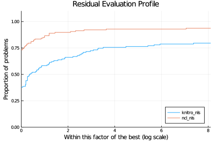
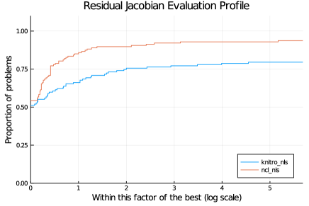
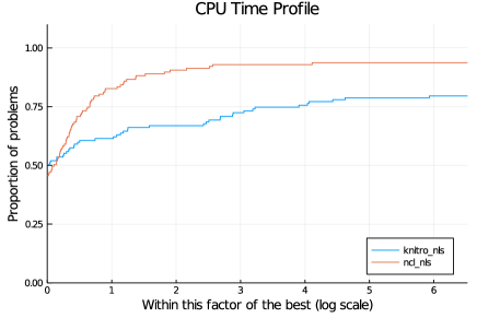
Figure 1: Performance profiles comparing knitro_nls (KNITRO’s NLS solver applied to (2)) and ncl_nls (KNITRO solving NC₀) on 127 nonlinear least squares problems from CUTEst. ncl_nls is more efficient.

6 Summary

Our AMPL implementation of the tax policy models and Algorithm NCL has been the only way we could handle these particular problems reliably [15], with KNITRO solving each subproblem accurately. Our Julia implementation of NCL achieves greater efficiency on these AMPL models by gradually tightening the KNITRO feasibility and optimality tolerances. It also permits testing on a broad range of problems, as illustrated on nonlinear least-squares problems and other problems from the CUTEst test set. We believe Algorithm NCL could become an effective general-purpose optimization solver when first and second derivatives are available. It is especially useful when the LICQ is not satisfied at the solution. The current Julia implementation of NCL (with KNITRO as subproblem solver) is not quite competitive with KNITRO itself on the general CUTEst problems in terms of run-time or number of evaluations, but it does solve some problems on which KNITRO fails. An advantage is that the implementation is generic and may be applied to problems from any collection adhering to the interface of the NLPModels.jl package [24].

Appendix A Detailed results for Julia/NCL on NLS problems

Table LABEL:tab:knitro-nls reports the detailed results of KNITRO/Levenberg-Marquardt on problems of the form (2) using the modeling mechanism of Section 5. In the table headers, ‘‘nvar’’ is the number of variables, ‘‘ncon’’ is the number of constraints (i.e., the number of least-squares residuals), $f$ is the final objective value, $\|\nabla L\|_{2}$ is the final dual residual, $t$ is the run-time in seconds, ‘‘iter’’ is the number of iterations, ‘‘#$c$’’ is the number of constraint (i.e, residual) evaluations, ‘‘#$\nabla c$’’ is the number of constraint (i.e., residual) Jacobian evaluations, and ‘‘status’’ is the final solver status.

Table LABEL:tab:ncl-nls reports the results of Julia/NCL solving Problem NC₀ for the same models. In the interest of space, the second table does not repeat problem dimensions. The other columns are as follows: $\|c\|_{2}$ is the final primal feasibility, and $\#\nabla^{2}L$ is the number of Hessian evaluations.

Table 10: knitro_nls results on $127$ CUTEst nonlinear least-squares problems. $101$ problems were solved successfully.

name	nvar	ncon	$f$	$\|\nabla L\|_{2}$	$t$	iter	#$c$	#$\nabla c$	status
ARWHDNE	$500$	$998$	$6.971$e$+01$	$8.5$e$-06$	$0.46$	$22$	$167$	$23$	first_order
BA-L1	$57$	$12$	$1.204$e$-25$	$3.8$e$-10$	$0.00$	$5$	$6$	$6$	first_order
BA-L16	$66462$	$167436$	$4.243$e$+05$	$4.2$e$-04$	$69.92$	$27$	$30$	$28$	first_order
BA-L1SP	$57$	$12$	$1.620$e$-23$	$5.1$e$-09$	$0.01$	$5$	$6$	$6$	first_order
BA-L21	$34134$	$72910$	$1.975$e$+05$	$7.2$e$-05$	$129.28$	$119$	$160$	$120$	first_order
BA-L49	$23769$	$63686$	$1.241$e$+05$	$4.0$e$+05$	$1809.44$	$121$	$728$	$122$	max_time
BA-L52	$192627$	$694346$	$2.147$e$+06$	$3.9$e$+07$	$1808.91$	$37$	$200$	$38$	max_time
BA-L73	$33753$	$92244$	$6.312$e$+05$	$9.5$e$+06$	$1801.24$	$396$	$2312$	$397$	max_time
BARDNE	$3$	$15$	$4.107$e$-03$	$2.7$e$-09$	$0.00$	$5$	$6$	$6$	first_order
BDQRTICNE	$5000$	$9992$	$1.000$e$+04$	$1.4$e$-01$	$91.67$	$500$	$3668$	$501$	max_iter
BEALENE	$2$	$3$	$1.491$e$-25$	$2.6$e$-12$	$0.00$	$6$	$8$	$7$	first_order
BIGGS6NE	$6$	$13$	$2.367$e$-17$	$5.9$e$-09$	$0.01$	$30$	$124$	$31$	first_order
BOX3NE	$3$	$10$	$3.259$e$-19$	$3.9$e$-10$	$0.00$	$5$	$6$	$6$	first_order
BROWNBSNE	$2$	$3$	$0.000$e$+00$	$0.0$e$+00$	$0.00$	$12$	$53$	$13$	first_order
BROWNDENE	$4$	$20$	$4.291$e$+04$	$2.4$e$+00$	$0.09$	$500$	$1697$	$501$	max_iter
BRYBNDNE	$5000$	$5000$	$1.499$e$-21$	$8.2$e$-11$	$1.16$	$6$	$7$	$7$	first_order
CHAINWOONE	$4000$	$11994$	$4.699$e$+03$	$5.9$e$+01$	$63.96$	$500$	$1339$	$501$	max_iter
CHEBYQADNE	$100$	$100$	$4.749$e$-03$	$1.5$e$-04$	$7.53$	$500$	$1994$	$501$	max_iter
CHNRSBNE	$50$	$98$	$7.394$e$-18$	$3.2$e$-08$	$0.01$	$38$	$78$	$39$	first_order
CHNRSNBMNE	$50$	$98$	$1.452$e$-20$	$1.8$e$-09$	$0.02$	$54$	$132$	$55$	first_order
COATINGNE	$134$	$252$	$2.527$e$-01$	$5.5$e$-07$	$0.01$	$9$	$11$	$10$	first_order
CUBENE	$2$	$2$	$1.085$e$-26$	$1.1$e$-13$	$0.00$	$4$	$9$	$5$	first_order
DECONVBNE	$63$	$40$	$4.542$e$-10$	$6.0$e$-07$	$0.03$	$54$	$214$	$55$	first_order
DECONVNE	$63$	$40$	$2.245$e$-16$	$8.5$e$-10$	$0.00$	$2$	$3$	$3$	first_order
DENSCHNBNE	$2$	$3$	$8.573$e$-27$	$1.9$e$-13$	$0.00$	$5$	$6$	$6$	first_order
DENSCHNCNE	$2$	$2$	$2.838$e$-22$	$8.4$e$-11$	$0.00$	$7$	$8$	$8$	first_order
DENSCHNDNE	$3$	$3$	$8.307$e$-10$	$5.5$e$-07$	$0.00$	$17$	$18$	$18$	first_order
DENSCHNENE	$3$	$3$	$3.005$e$-22$	$2.4$e$-11$	$0.00$	$8$	$19$	$9$	first_order
DENSCHNFNE	$2$	$2$	$1.392$e$-26$	$2.1$e$-12$	$0.00$	$5$	$6$	$6$	first_order
DEVGLA1NE	$4$	$24$	$1.063$e$-13$	$2.4$e$-08$	$0.00$	$11$	$31$	$12$	first_order
DEVGLA2NE	$5$	$16$	$4.828$e$-15$	$5.9$e$-07$	$0.00$	$9$	$16$	$10$	first_order
EGGCRATENE	$2$	$4$	$4.744$e$+00$	$9.6$e$-07$	$0.00$	$5$	$6$	$6$	first_order
ELATVIDUNE	$2$	$3$	$2.738$e$+01$	$3.2$e$-06$	$0.00$	$15$	$30$	$16$	first_order
ENGVAL2NE	$3$	$5$	$2.465$e$-32$	$2.2$e$-16$	$0.00$	$10$	$14$	$11$	first_order
ERRINROSNE	$50$	$98$	$2.020$e$+01$	$1.8$e$-05$	$0.01$	$45$	$63$	$46$	first_order
ERRINRSMNE	$50$	$98$	$1.926$e$+01$	$1.7$e$-05$	$0.01$	$44$	$66$	$45$	first_order
EXP2NE	$2$	$10$	$1.618$e$-19$	$8.7$e$-12$	$0.00$	$5$	$6$	$6$	first_order
EXPFITNE	$2$	$10$	$1.203$e$-01$	$4.9$e$-07$	$0.00$	$10$	$12$	$11$	first_order
EXTROSNBNE	$1000$	$999$	$8.071$e$-31$	$1.3$e$-14$	$0.07$	$6$	$14$	$7$	first_order
FBRAIN2NE	$4$	$2211$	$1.842$e$-01$	$6.8$e$-07$	$0.08$	$8$	$11$	$9$	first_order
FBRAINNE	$2$	$2211$	$2.083$e$-01$	$5.7$e$-07$	$0.02$	$5$	$6$	$6$	first_order
FREURONE	$2$	$2$	$2.449$e$+01$	$1.8$e$-05$	$0.01$	$19$	$102$	$20$	first_order
GENROSEBNE	$500$	$998$	$7.965$e$+02$	$3.6$e$-06$	$0.04$	$8$	$10$	$10$	first_order
GENROSENE	$1000$	$1999$	$1.247$e$+02$	$6.3$e$+00$	$3.40$	$500$	$1567$	$501$	max_iter
GULFNE	$3$	$99$	$2.107$e$-01$	$4.0$e$+06$	$0.27$	$500$	$2578$	$501$	max_iter
HATFLDANE	$4$	$4$	$2.172$e$-17$	$3.4$e$-09$	$0.00$	$8$	$10$	$9$	first_order
HATFLDBNE	$4$	$4$	$2.786$e$-03$	$1.4$e$-07$	$0.00$	$7$	$8$	$8$	first_order
HATFLDCNE	$25$	$25$	$1.018$e$-15$	$1.5$e$-08$	$0.00$	$3$	$4$	$4$	first_order
HATFLDDNE	$3$	$10$	$1.273$e$-07$	$7.1$e$-11$	$0.00$	$6$	$9$	$7$	first_order
HATFLDENE	$3$	$21$	$1.364$e$-06$	$8.2$e$-12$	$0.00$	$5$	$6$	$6$	first_order
HATFLDFLNE	$3$	$3$	$3.254$e$-05$	$9.1$e$-07$	$0.01$	$11$	$69$	$12$	first_order
HELIXNE	$3$	$3$	$2.195$e$-20$	$2.8$e$-09$	$0.00$	$9$	$11$	$10$	first_order
HIMMELBFNE	$4$	$7$	$1.593$e$+06$	$4.4$e$-04$	$0.01$	$28$	$66$	$29$	first_order
HS1NE	$2$	$2$	$3.274$e$-17$	$4.0$e$-09$	$0.00$	$9$	$20$	$10$	first_order
HS25NE	$3$	$99$	$1.642$e$+01$	$9.2$e$-09$	$0.00$	$0$	$1$	$1$	first_order
HS2NE	$2$	$2$	$2.471$e$+00$	$2.1$e$-08$	$0.00$	$6$	$8$	$8$	first_order
INTEQNE	$12$	$12$	$6.938$e$-14$	$2.1$e$-07$	$0.00$	$2$	$3$	$3$	first_order
JENSMPNE	$2$	$10$	$6.218$e$+01$	$7.1$e$-06$	$0.01$	$10$	$82$	$11$	first_order
JUDGENE	$2$	$20$	$8.041$e$+00$	$1.2$e$-06$	$0.00$	$9$	$10$	$10$	first_order
KOEBHELBNE	$3$	$156$	$3.876$e$+01$	$7.5$e$-07$	$0.10$	$194$	$757$	$195$	first_order
KOWOSBNE	$4$	$11$	$1.539$e$-04$	$6.9$e$-07$	$0.00$	$16$	$30$	$17$	first_order
LIARWHDNE	$5000$	$10000$	$1.608$e$-27$	$4.4$e$-12$	$1.07$	$5$	$6$	$6$	first_order
LINVERSENE	$1999$	$2997$	$3.405$e$+02$	$1.2$e$-02$	$13.28$	$500$	$1753$	$502$	max_iter
MANCINONE	$100$	$100$	$7.966$e$-22$	$2.2$e$-08$	$0.10$	$5$	$6$	$6$	first_order
MANNE	$6000$	$4000$	$3.261$e$+39$	$1.4$e$+19$	$95.71$	$167$	$168$	$168$	unknown
MARINE	$11215$	$11192$	$3.922$e$-21$	$8.0$e$-08$	$8.51$	$9$	$10$	$10$	first_order
MEYER3NE	$3$	$16$	$4.397$e$+01$	$1.1$e$-03$	$0.00$	$11$	$19$	$12$	unknown
MODBEALENE	$20000$	$39999$	$1.374$e$+00$	$8.3$e$-07$	$109.80$	$38$	$73$	$39$	first_order
MOREBVNE	$10$	$10$	$1.085$e$-14$	$1.9$e$-08$	$0.00$	$2$	$3$	$3$	first_order
MUONSINE	$1$	$512$	$2.194$e$+04$	$8.8$e$-04$	$0.02$	$36$	$37$	$37$	first_order
NGONE	$200$	$5048$	$7.203$e$-13$	$8.3$e$-07$	$36.90$	$221$	$914$	$223$	first_order
NONDIANE	$5000$	$5000$	$4.949$e$-01$	$1.9$e$-08$	$2.63$	$16$	$39$	$17$	first_order
NONMSQRTNE	$4900$	$4900$	$3.543$e$+02$	$1.1$e$+01$	$154.67$	$500$	$2624$	$501$	max_iter
NONSCOMPNE	$5000$	$5000$	$1.378$e$-06$	$5.6$e$-07$	$11.31$	$80$	$217$	$81$	first_order
OSCIGRNE	$100000$	$100000$	$3.138$e$-24$	$8.3$e$-09$	$3.62$	$7$	$8$	$8$	first_order
OSCIPANE	$10$	$10$	$5.000$e$-01$	$1.1$e$-01$	$0.11$	$500$	$2880$	$501$	max_iter
PALMER1ANE	$6$	$35$	$4.494$e$-02$	$6.7$e$-07$	$0.01$	$25$	$84$	$26$	first_order
PALMER1BNE	$4$	$35$	$1.724$e$+00$	$2.6$e$-08$	$0.00$	$6$	$7$	$7$	first_order
PALMER1ENE	$8$	$35$	$1.822$e$-01$	$1.3$e$+02$	$0.17$	$500$	$3471$	$501$	max_iter
PALMER1NE	$4$	$31$	$5.877$e$+03$	$8.4$e$+00$	$0.13$	$500$	$2561$	$501$	max_iter
PALMER2ANE	$6$	$23$	$8.555$e$-03$	$5.9$e$-07$	$0.02$	$58$	$248$	$59$	first_order
PALMER2BNE	$4$	$23$	$3.116$e$-01$	$5.2$e$-08$	$0.00$	$8$	$10$	$9$	first_order
PALMER2ENE	$8$	$23$	$1.952$e$-02$	$8.9$e$-07$	$0.01$	$9$	$68$	$10$	first_order
PALMER2NE	$4$	$23$	$1.826$e$+03$	$4.1$e$-06$	$0.01$	$26$	$92$	$27$	unknown
PALMER3ANE	$6$	$23$	$1.022$e$-02$	$1.0$e$-07$	$0.00$	$18$	$39$	$19$	first_order
PALMER3BNE	$4$	$23$	$2.114$e$+00$	$1.5$e$-07$	$0.00$	$11$	$14$	$12$	first_order
PALMER3ENE	$8$	$23$	$2.303$e$-02$	$1.2$e$+01$	$0.15$	$500$	$3348$	$501$	max_iter
PALMER3NE	$4$	$23$	$1.133$e$+03$	$5.7$e$-02$	$0.15$	$500$	$3303$	$501$	max_iter
PALMER4ANE	$6$	$23$	$2.030$e$-02$	$3.8$e$-07$	$0.03$	$98$	$445$	$99$	first_order
PALMER4BNE	$4$	$23$	$3.418$e$+00$	$6.1$e$-07$	$0.00$	$14$	$18$	$15$	first_order
PALMER4ENE	$8$	$23$	$6.286$e$-02$	$9.3$e$-07$	$0.04$	$69$	$667$	$70$	first_order
PALMER4NE	$4$	$23$	$1.143$e$+03$	$2.2$e$-05$	$0.01$	$35$	$163$	$36$	unknown
PALMER5ANE	$8$	$12$	$1.706$e$-01$	$1.2$e$+00$	$0.13$	$500$	$3000$	$501$	max_iter
PALMER5BNE	$9$	$12$	$4.876$e$-03$	$3.4$e$-07$	$0.03$	$93$	$481$	$94$	first_order
PALMER5ENE	$8$	$12$	$1.699$e$-02$	$1.4$e$+00$	$0.16$	$500$	$3508$	$501$	max_iter
PALMER6ANE	$6$	$13$	$2.797$e$-02$	$2.3$e$-07$	$0.00$	$17$	$30$	$18$	first_order
PALMER6ENE	$8$	$13$	$2.424$e$-02$	$5.8$e$-07$	$0.08$	$142$	$1654$	$143$	first_order
PALMER7ANE	$6$	$13$	$5.526$e$+00$	$2.4$e$+00$	$0.13$	$500$	$2806$	$501$	max_iter
PALMER7ENE	$8$	$13$	$3.353$e$+00$	$1.4$e$+02$	$0.16$	$500$	$3243$	$500$	max_iter
PALMER8ANE	$6$	$12$	$3.700$e$-02$	$5.8$e$-07$	$0.02$	$72$	$303$	$73$	first_order
PALMER8ENE	$8$	$12$	$1.687$e$-01$	$2.3$e$-04$	$0.22$	$500$	$5007$	$501$	max_iter
PENLT1NE	$10$	$11$	$3.576$e$-10$	$8.1$e$-07$	$0.02$	$111$	$385$	$112$	first_order
PENLT2NE	$4$	$8$	$4.701$e$-11$	$9.6$e$-07$	$0.03$	$163$	$613$	$164$	first_order
PINENE	$8805$	$8795$	$5.184$e$-17$	$1.1$e$-07$	$1.72$	$2$	$10$	$3$	first_order
POWERSUMNE	$4$	$4$	$2.325$e$-17$	$7.6$e$-07$	$0.00$	$17$	$21$	$18$	first_order
PRICE3NE	$2$	$2$	$5.614$e$-22$	$3.9$e$-10$	$0.00$	$7$	$8$	$8$	first_order
PRICE4NE	$2$	$2$	$1.321$e$-14$	$9.8$e$-07$	$0.00$	$21$	$22$	$22$	first_order
QINGNE	$100$	$100$	$9.461$e$-20$	$1.2$e$-09$	$0.00$	$5$	$8$	$6$	first_order
RSNBRNE	$2$	$2$	$4.832$e$-30$	$3.1$e$-15$	$0.00$	$11$	$34$	$12$	first_order
S308NE	$2$	$3$	$3.866$e$-01$	$9.1$e$-07$	$0.00$	$34$	$36$	$35$	first_order
SBRYBNDNE	$5000$	$5000$	$1.790$e$-21$	$3.0$e$-07$	$1.16$	$6$	$7$	$7$	first_order
SINVALNE	$2$	$2$	$3.852$e$-32$	$2.8$e$-15$	$0.00$	$4$	$11$	$5$	first_order
SPECANNE	$9$	$15000$	$3.291$e$-13$	$5.3$e$-08$	$0.08$	$6$	$7$	$7$	first_order
SROSENBRNE	$5000$	$5000$	$5.547$e$-28$	$6.7$e$-16$	$0.49$	$2$	$3$	$3$	first_order
SSBRYBNDNE	$5000$	$5000$	$5.274$e$-22$	$4.0$e$-10$	$1.15$	$6$	$7$	$7$	first_order
STREGNE	$4$	$2$	$2.236$e$-03$	$4.7$e$-01$	$0.05$	$500$	$535$	$501$	max_iter
STRTCHDVNE	$10$	$9$	$3.723$e$-10$	$4.4$e$-07$	$0.00$	$8$	$9$	$9$	first_order
TQUARTICNE	$5000$	$5000$	$2.631$e$-26$	$2.3$e$-13$	$0.39$	$1$	$2$	$2$	first_order
TRIGON1NE	$10$	$10$	$6.724$e$-16$	$1.0$e$-07$	$0.00$	$4$	$5$	$5$	first_order
TRIGON2NE	$10$	$31$	$1.620$e$+00$	$1.5$e$-09$	$0.00$	$7$	$8$	$8$	first_order
VARDIMNE	$10$	$12$	$7.960$e$-16$	$4.0$e$-07$	$0.00$	$9$	$10$	$10$	first_order
VIBRBEAMNE	$8$	$30$	$7.822$e$-02$	$6.9$e$-07$	$0.00$	$10$	$11$	$11$	first_order
WATSONNE	$12$	$31$	$1.429$e$-15$	$1.3$e$-13$	$0.00$	$4$	$5$	$5$	first_order
WAYSEA1NE	$2$	$2$	$3.683$e$-16$	$8.7$e$-07$	$0.00$	$7$	$8$	$8$	first_order
WAYSEA2NE	$2$	$2$	$3.388$e$-18$	$1.3$e$-08$	$0.00$	$11$	$17$	$12$	first_order
WEEDSNE	$3$	$12$	$1.294$e$+00$	$3.0$e$-07$	$0.00$	$15$	$25$	$16$	first_order
WOODSNE	$4000$	$3001$	$5.000$e$-01$	$0.0$e$+00$	$0.33$	$2$	$3$	$3$	first_order

Table 11: ncl_nls results on $127$ CUTEst nonlinear least-squares problems. 119 problems were solved successfully.

name	$f$	$\|\nabla L\|_{2}$	$\|c\|_{2}$	$t$	iter	#$c$	#$\nabla c$	#$\nabla^{2}L$	status
ARWHDNE	$6.971$e$+01$	$1.5$e$-14$	$1.4$e$-16$	$2.65$	$30$	$105$	$32$	$31$	first_order
BA-L1	$4.400$e$-31$	$9.1$e$-16$	$2.0$e$-10$	$0.01$	$5$	$6$	$7$	$6$	first_order
BA-L16	$4.324$e$+05$	$1.4$e$+03$	$4.5$e$-07$	$937.15$	$88$	$454$	$90$	$89$	unknown
BA-L1SP	$3.204$e$-23$	$7.4$e$-12$	$8.3$e$-05$	$0.01$	$4$	$5$	$6$	$5$	first_order
BA-L21	$1.975$e$+05$	$1.5$e$-02$	$3.0$e$-05$	$947.20$	$201$	$1093$	$203$	$203$	max_time
BA-L49	$1.674$e$+04$	$1.2$e$-01$	$1.6$e$-04$	$869.15$	$217$	$1189$	$219$	$219$	max_time
BA-L52	$3.860$e$+06$	$2.0$e$+02$	$8.0$e$-01$	$1778.45$	$31$	$50$	$33$	$32$	max_time
BA-L73	$9.609$e$+05$	$1.1$e$+02$	$1.9$e$-06$	$693.06$	$135$	$635$	$137$	$136$	unknown
BARDNE	$4.107$e$-03$	$2.3$e$-14$	$5.7$e$-12$	$0.00$	$5$	$6$	$7$	$6$	first_order
BDQRTICNE	$1.000$e$+04$	$3.4$e$-10$	$1.7$e$-11$	$0.47$	$17$	$25$	$19$	$18$	first_order
BEALENE	$4.598$e$-20$	$2.0$e$-10$	$1.6$e$-09$	$0.00$	$8$	$9$	$10$	$9$	first_order
BIGGS6NE	$2.153$e$-17$	$6.8$e$-12$	$7.2$e$-08$	$0.02$	$60$	$74$	$62$	$61$	first_order
BOX3NE	$2.641$e$-19$	$7.3$e$-12$	$1.8$e$-10$	$0.00$	$5$	$6$	$7$	$6$	first_order
BROWNBSNE	$5.933$e$-33$	$5.6$e$-12$	$1.1$e$-10$	$0.00$	$13$	$42$	$15$	$14$	first_order
BROWNDENE	$4.291$e$+04$	$9.7$e$-09$	$3.0$e$-11$	$0.00$	$14$	$22$	$16$	$15$	first_order
BRYBNDNE	$6.662$e$-20$	$2.6$e$-10$	$2.5$e$-10$	$0.20$	$6$	$7$	$8$	$7$	first_order
CHAINWOONE	$6.598$e$+03$	$1.8$e$+00$	$2.1$e$-01$	$14.40$	$500$	$546$	$502$	$501$	max_iter
CHEBYQADNE	$4.358$e$-03$	$5.1$e$-07$	$2.9$e$-07$	$0.60$	$33$	$51$	$35$	$34$	first_order
CHNRSBNE	$2.913$e$-21$	$1.9$e$-10$	$7.2$e$-11$	$0.02$	$34$	$51$	$36$	$35$	first_order
CHNRSNBMNE	$6.544$e$-23$	$4.0$e$-11$	$3.9$e$-10$	$0.02$	$38$	$57$	$40$	$39$	first_order
COATINGNE	$2.527$e$-01$	$1.5$e$-09$	$3.9$e$-10$	$0.02$	$11$	$22$	$13$	$12$	first_order
CUBENE	$2.479$e$-33$	$9.6$e$-17$	$6.7$e$-15$	$0.00$	$2$	$7$	$4$	$3$	first_order
DECONVBNE	$1.285$e$-03$	$3.1$e$-07$	$5.3$e$-06$	$0.03$	$20$	$34$	$23$	$21$	first_order
DECONVNE	$2.694$e$-15$	$3.8$e$-08$	$6.4$e$-10$	$0.00$	$2$	$3$	$4$	$3$	first_order
DENSCHNBNE	$1.225$e$-17$	$2.6$e$-09$	$5.8$e$-09$	$0.00$	$6$	$8$	$8$	$7$	first_order
DENSCHNCNE	$9.992$e$-38$	$4.3$e$-19$	$6.7$e$-06$	$0.00$	$6$	$7$	$8$	$7$	first_order
DENSCHNDNE	$4.012$e$-28$	$4.5$e$-17$	$3.6$e$-04$	$0.00$	$15$	$16$	$17$	$16$	first_order
DENSCHNENE	$4.540$e$-21$	$9.5$e$-11$	$1.7$e$-06$	$0.00$	$15$	$20$	$17$	$16$	first_order
DENSCHNFNE	$2.351$e$-38$	$2.2$e$-19$	$1.9$e$-06$	$0.00$	$4$	$5$	$6$	$5$	first_order
DEVGLA1NE	$1.063$e$-13$	$2.9$e$-08$	$4.0$e$-11$	$0.01$	$16$	$45$	$18$	$17$	first_order
DEVGLA2NE	$1.672$e$-14$	$6.3$e$-08$	$3.0$e$-07$	$0.00$	$9$	$12$	$11$	$10$	first_order
EGGCRATENE	$4.744$e$+00$	$3.1$e$-08$	$2.4$e$-09$	$0.00$	$4$	$5$	$6$	$5$	first_order
ELATVIDUNE	$2.738$e$+01$	$1.2$e$-09$	$5.0$e$-10$	$0.00$	$8$	$9$	$10$	$9$	first_order
ENGVAL2NE	$6.374$e$-15$	$1.3$e$-08$	$1.2$e$-07$	$0.00$	$12$	$20$	$14$	$13$	first_order
ERRINROSNE	$2.020$e$+01$	$1.4$e$-09$	$4.1$e$-10$	$0.01$	$17$	$24$	$19$	$18$	first_order
ERRINRSMNE	$1.926$e$+01$	$1.7$e$-08$	$1.2$e$-09$	$0.02$	$25$	$38$	$27$	$26$	first_order
EXP2NE	$1.617$e$-19$	$7.1$e$-13$	$1.9$e$-13$	$0.00$	$5$	$6$	$7$	$6$	first_order
EXPFITNE	$1.203$e$-01$	$2.4$e$-10$	$4.9$e$-12$	$0.01$	$21$	$149$	$23$	$22$	first_order
EXTROSNBNE	$-2.002$e$+00$	$1.0$e$-06$	$1.3$e$-09$	$1.16$	$250$	$1860$	$252$	$251$	first_order
FBRAIN2NE	$1.842$e$-01$	$6.3$e$-10$	$3.1$e$-11$	$0.11$	$5$	$6$	$7$	$6$	first_order
FBRAINNE	$2.083$e$-01$	$8.4$e$-08$	$1.7$e$-09$	$0.05$	$4$	$5$	$6$	$5$	first_order
FREURONE	$2.449$e$+01$	$1.5$e$-10$	$5.5$e$-12$	$0.00$	$7$	$15$	$9$	$8$	first_order
GENROSEBNE	$7.965$e$+02$	$1.3$e$-06$	$1.5$e$-06$	$0.04$	$6$	$8$	$9$	$7$	first_order
GENROSENE	$5.000$e$-01$	$8.9$e$-14$	$1.1$e$-14$	$2.07$	$436$	$639$	$438$	$437$	first_order
GULFNE	$1.755$e$-20$	$3.4$e$-11$	$1.6$e$-10$	$0.02$	$20$	$28$	$22$	$21$	first_order
HATFLDANE	$8.445$e$-20$	$5.4$e$-11$	$6.2$e$-09$	$0.00$	$9$	$10$	$11$	$10$	first_order
HATFLDBNE	$2.786$e$-03$	$4.8$e$-12$	$1.1$e$-11$	$0.00$	$7$	$8$	$9$	$8$	first_order
HATFLDCNE	$2.674$e$-17$	$4.6$e$-09$	$7.8$e$-09$	$0.00$	$3$	$4$	$5$	$4$	first_order
HATFLDDNE	$1.273$e$-07$	$4.1$e$-09$	$9.7$e$-07$	$0.00$	$5$	$8$	$7$	$6$	first_order
HATFLDENE	$1.364$e$-06$	$5.8$e$-11$	$1.7$e$-09$	$0.00$	$5$	$6$	$7$	$6$	first_order
HATFLDFLNE	$3.008$e$-05$	$9.2$e$-12$	$7.3$e$-09$	$0.02$	$103$	$443$	$105$	$104$	first_order
HELIXNE	$5.661$e$-43$	$1.7$e$-21$	$1.7$e$-10$	$0.00$	$9$	$12$	$11$	$10$	first_order
HIMMELBFNE	$2.168$e$+06$	$2.1$e$+02$	$2.9$e$-04$	$0.09$	$500$	$720$	$502$	$501$	max_iter
HS1NE	$3.359$e$-17$	$4.1$e$-09$	$5.8$e$-16$	$0.00$	$7$	$11$	$9$	$8$	first_order
HS25NE	$1.642$e$+01$	$8.1$e$-08$	$3.6$e$-11$	$0.00$	$3$	$5$	$6$	$4$	first_order
HS2NE	$2.471$e$+00$	$8.4$e$-12$	$1.3$e$-12$	$0.00$	$5$	$7$	$8$	$6$	first_order
INTEQNE	$6.816$e$-37$	$8.7$e$-19$	$1.6$e$-07$	$0.00$	$2$	$3$	$4$	$3$	first_order
JENSMPNE	$6.218$e$+01$	$1.6$e$-08$	$3.1$e$-09$	$0.00$	$8$	$14$	$10$	$9$	first_order
JUDGENE	$8.041$e$+00$	$4.8$e$-07$	$2.5$e$-07$	$0.00$	$5$	$6$	$7$	$6$	first_order
KOEBHELBNE	$3.876$e$+01$	$1.4$e$-08$	$4.5$e$-09$	$0.13$	$119$	$164$	$121$	$121$	first_order
KOWOSBNE	$1.539$e$-04$	$2.9$e$-10$	$2.6$e$-09$	$0.00$	$11$	$14$	$13$	$12$	first_order
LIARWHDNE	$1.113$e$-21$	$4.7$e$-11$	$4.0$e$-11$	$0.17$	$6$	$7$	$8$	$7$	first_order
LINVERSENE	$3.405$e$+02$	$3.3$e$-07$	$1.4$e$-07$	$0.31$	$19$	$22$	$22$	$20$	first_order
MANCINONE	$2.507$e$-32$	$1.1$e$-16$	$2.4$e$-09$	$0.12$	$4$	$5$	$6$	$5$	first_order
MANNE	$-9.698$e$-01$	$9.6$e$-07$	$0.0$e$+00$	$10.27$	$344$	$346$	$347$	$345$	first_order
MARINE	$2.009$e$+06$	$1.7$e$-08$	$1.1$e$-08$	$3.76$	$40$	$43$	$43$	$41$	first_order
MEYER3NE	$4.397$e$+01$	$2.0$e$-06$	$1.1$e$-08$	$0.00$	$8$	$14$	$10$	$9$	first_order
MODBEALENE	$2.521$e$-18$	$1.5$e$-09$	$2.8$e$-09$	$1.80$	$11$	$12$	$13$	$12$	first_order
MOREBVNE	$2.674$e$-37$	$9.3$e$-19$	$7.6$e$-08$	$0.00$	$2$	$3$	$4$	$3$	first_order
MUONSINE	$2.194$e$+04$	$2.4$e$-11$	$6.2$e$-14$	$0.02$	$10$	$15$	$12$	$11$	first_order
NGONE	$-8.551$e$+00$	$4.0$e$-09$	$3.8$e$-11$	$2.46$	$106$	$108$	$109$	$107$	first_order
NONDIANE	$4.949$e$-01$	$1.3$e$-16$	$1.5$e$-07$	$0.16$	$6$	$7$	$8$	$7$	first_order
NONMSQRTNE	$3.543$e$+02$	$1.1$e$-07$	$2.5$e$-06$	$4.01$	$19$	$30$	$21$	$20$	first_order
NONSCOMPNE	$1.805$e$-07$	$1.8$e$-10$	$3.0$e$-06$	$0.52$	$19$	$28$	$21$	$20$	first_order
OSCIGRNE	$1.449$e$-35$	$4.0$e$-18$	$1.4$e$-07$	$3.78$	$6$	$7$	$8$	$7$	first_order
OSCIPANE	$5.000$e$-01$	$9.8$e$-06$	$5.5$e$-04$	$0.16$	$500$	$2698$	$502$	$501$	max_iter
PALMER1ANE	$2.988$e$+01$	$2.4$e$-06$	$6.8$e$-08$	$0.01$	$12$	$16$	$14$	$13$	first_order
PALMER1BNE	$1.724$e$+00$	$1.9$e$-08$	$1.9$e$-10$	$0.01$	$11$	$16$	$13$	$12$	first_order
PALMER1ENE	$4.176$e$-04$	$7.7$e$-09$	$1.4$e$-06$	$0.00$	$7$	$8$	$9$	$8$	first_order
PALMER1NE	$5.877$e$+03$	$2.7$e$-06$	$2.4$e$-09$	$0.02$	$37$	$46$	$39$	$38$	first_order
PALMER2ANE	$8.555$e$-03$	$1.9$e$-10$	$4.1$e$-08$	$0.02$	$44$	$69$	$46$	$45$	first_order
PALMER2BNE	$3.116$e$-01$	$1.9$e$-07$	$3.1$e$-09$	$0.00$	$8$	$11$	$10$	$9$	first_order
PALMER2ENE	$5.815$e$-02$	$6.9$e$-08$	$3.2$e$-10$	$0.01$	$20$	$23$	$22$	$21$	first_order
PALMER2NE	$1.826$e$+03$	$3.4$e$-06$	$5.3$e$-08$	$0.02$	$49$	$64$	$51$	$50$	first_order
PALMER3ANE	$1.022$e$-02$	$2.0$e$-08$	$9.0$e$-07$	$0.01$	$13$	$17$	$15$	$14$	first_order
PALMER3BNE	$2.114$e$+00$	$6.1$e$-12$	$1.1$e$-14$	$0.01$	$27$	$38$	$29$	$28$	first_order
PALMER3ENE	$2.537$e$-05$	$4.1$e$-11$	$1.2$e$-09$	$0.01$	$14$	$19$	$16$	$15$	first_order
PALMER3NE	$1.208$e$+03$	$1.1$e$-05$	$2.4$e$-08$	$0.00$	$6$	$10$	$8$	$7$	first_order
PALMER4ANE	$2.030$e$-02$	$2.8$e$-08$	$1.6$e$-07$	$0.01$	$11$	$20$	$13$	$12$	first_order
PALMER4BNE	$3.418$e$+00$	$1.3$e$-12$	$2.3$e$-14$	$0.01$	$32$	$41$	$34$	$33$	first_order
PALMER4ENE	$7.400$e$-05$	$4.7$e$-09$	$2.0$e$-07$	$0.01$	$11$	$13$	$13$	$12$	first_order
PALMER4NE	$1.212$e$+03$	$1.5$e$-05$	$4.2$e$-08$	$0.00$	$6$	$10$	$8$	$7$	first_order
PALMER5ANE	$1.452$e$-02$	$9.5$e$-07$	$4.3$e$-07$	$0.10$	$182$	$874$	$184$	$183$	first_order
PALMER5BNE	$4.876$e$-03$	$3.7$e$-09$	$1.1$e$-07$	$0.01$	$44$	$50$	$46$	$45$	first_order
PALMER5ENE	$1.036$e$-02$	$1.3$e$-09$	$3.3$e$-07$	$0.02$	$60$	$200$	$62$	$61$	first_order
PALMER6ANE	$2.797$e$-02$	$2.1$e$-08$	$7.5$e$-06$	$0.01$	$22$	$31$	$24$	$23$	first_order
PALMER6ENE	$6.462$e$-02$	$5.5$e$-07$	$2.3$e$-06$	$0.00$	$7$	$10$	$9$	$8$	first_order
PALMER7ANE	$5.168$e$+00$	$1.6$e$-07$	$2.6$e$-05$	$0.16$	$355$	$1551$	$357$	$358$	first_order
PALMER7ENE	$3.346$e$+00$	$1.5$e$-06$	$4.0$e$-10$	$0.03$	$54$	$274$	$56$	$55$	first_order
PALMER8ANE	$3.700$e$-02$	$9.3$e$-08$	$3.6$e$-07$	$0.01$	$19$	$31$	$21$	$20$	first_order
PALMER8ENE	$3.170$e$-01$	$6.3$e$-08$	$3.3$e$-09$	$0.01$	$25$	$35$	$27$	$26$	first_order
PENLT1NE	$3.544$e$-10$	$5.5$e$-14$	$3.8$e$-05$	$0.00$	$8$	$9$	$10$	$9$	first_order
PENLT2NE	$4.688$e$-11$	$1.4$e$-18$	$5.6$e$-08$	$0.00$	$5$	$10$	$7$	$6$	first_order
PINENE	$4.194$e$-05$	$4.9$e$-10$	$1.1$e$-06$	$0.72$	$13$	$18$	$16$	$14$	first_order
POWERSUMNE	$1.799$e$-22$	$1.2$e$-11$	$6.0$e$-10$	$0.01$	$45$	$48$	$47$	$46$	first_order
PRICE3NE	$1.505$e$-35$	$5.2$e$-18$	$1.1$e$-05$	$0.00$	$6$	$7$	$8$	$7$	first_order
PRICE4NE	$3.508$e$-32$	$3.4$e$-19$	$1.1$e$-04$	$0.00$	$13$	$14$	$15$	$14$	first_order
QINGNE	$1.318$e$-33$	$2.8$e$-17$	$9.2$e$-05$	$0.00$	$4$	$7$	$6$	$5$	first_order
RSNBRNE	$5.556$e$-32$	$3.3$e$-16$	$3.1$e$-14$	$0.00$	$1$	$3$	$3$	$2$	first_order
S308NE	$3.866$e$-01$	$1.7$e$-09$	$9.0$e$-10$	$0.00$	$10$	$16$	$12$	$11$	first_order
SBRYBNDNE	$6.690$e$-20$	$2.6$e$-10$	$2.5$e$-10$	$0.18$	$6$	$7$	$8$	$7$	first_order
SINVALNE	$1.578$e$-30$	$1.8$e$-15$	$1.8$e$-15$	$0.00$	$1$	$3$	$3$	$2$	first_order
SPECANNE	$3.291$e$-13$	$3.5$e$-08$	$1.2$e$-12$	$0.49$	$10$	$14$	$12$	$11$	first_order
SROSENBRNE	$5.892$e$-33$	$1.1$e$-18$	$2.2$e$-18$	$0.05$	$2$	$3$	$4$	$3$	first_order
SSBRYBNDNE	$6.663$e$-20$	$2.6$e$-10$	$2.5$e$-10$	$0.21$	$6$	$7$	$8$	$7$	first_order
STREGNE	$2.204$e$-27$	$6.6$e$-22$	$4.4$e$-15$	$0.00$	$2$	$3$	$4$	$3$	first_order
STRTCHDVNE	$2.260$e$-15$	$1.8$e$-10$	$6.1$e$-07$	$0.00$	$10$	$11$	$12$	$11$	first_order
TQUARTICNE	$0.000$e$+00$	$0.0$e$+00$	$2.2$e$-16$	$0.05$	$1$	$2$	$3$	$2$	first_order
TRIGON1NE	$3.427$e$-39$	$5.7$e$-20$	$1.8$e$-08$	$0.00$	$4$	$5$	$6$	$5$	first_order
TRIGON2NE	$1.620$e$+00$	$2.7$e$-09$	$1.3$e$-09$	$0.00$	$11$	$12$	$13$	$12$	first_order
VARDIMNE	$4.873$e$-20$	$2.9$e$-09$	$1.2$e$-10$	$0.00$	$14$	$19$	$16$	$15$	first_order
VIBRBEAMNE	$7.822$e$-02$	$2.3$e$-11$	$1.7$e$-14$	$0.01$	$7$	$8$	$9$	$8$	first_order
WATSONNE	$1.430$e$-15$	$5.8$e$-16$	$5.6$e$-14$	$0.00$	$4$	$5$	$6$	$5$	first_order
WAYSEA1NE	$0.000$e$+00$	$0.0$e$+00$	$2.7$e$-08$	$0.00$	$7$	$8$	$9$	$8$	first_order
WAYSEA2NE	$8.386$e$-17$	$2.3$e$-09$	$1.0$e$-07$	$0.00$	$10$	$20$	$12$	$11$	first_order
WEEDSNE	$1.294$e$+00$	$8.6$e$-08$	$7.4$e$-07$	$0.01$	$17$	$24$	$19$	$18$	first_order
WOODSNE	$-1.906$e$+04$	$9.1$e$-13$	$8.0$e$-10$	$0.04$	$3$	$4$	$5$	$4$	first_order

References

- [1] AMPL modeling system. http://www.ampl.com.
- [2] Jon Bentley. Programming pearls: Little languages. Commun. ACM, 29(8):711--–721, August 1986.
- [3] Jeff Bezanson, Alan Edelman, Stefan Karpinski, and Viral B Shah. Julia: A fresh approach to numerical computing. SIAM Rev., 59(1):65--98, 2017.
- [4] A. R. Conn, N. I. M. Gould, and Ph. L. Toint. A globally convergent augmented Lagrangian algorithm for optimization with general constraints and simple bounds. SIAM J. Numer. Anal., 28:545--572, 1991.
- [5] A. R. Conn, N. I. M. Gould, and Ph. L. Toint. LANCELOT: A Fortran Package for Large-scale Nonlinear Optimization (Release A). Lecture Notes in Computation Mathematics 17. Springer Verlag, Berlin, Heidelberg, New York, London, Paris and Tokyo, 1992.
- [6] R. Fourer, D. M. Gay, and B. W. Kernighan. AMPL: A Modeling Language for Mathematical Programming. Brooks/Cole, Pacific Grove, second edition, 2002.
- [7] GAMS modeling system. http://www.gams.com.
- [8] P. E. Gill, W. Murray, and M. A. Saunders. SNOPT: An SQP algorithm for large-scale constrained optimization. SIAM Rev., 47(1):99--131, 2005. SIGEST article.
- [9] N. I. M. Gould, D. Orban, and Ph. L. Toint. CUTEst: a Constrained and Unconstrained Testing Environment with safe threads. Comput. Optim. Appl., 60:545--557, 2015.
- [10] COIN-OR Interior Point Optimizer IPOPT. https://github.com/coin-or/Ipopt.
- [11] K. L. Judd and C.-L. Su. Optimal income taxation with multidimensional taxpayer types. Working paper, Hoover Institution, Stanford University, 2011.
- [12] KNITRO optimization software. https://www.artelys.com/tools/knitro_doc/2_userGuide.html.
- [13] LANCELOT optimization software. http://www.numerical.rl.ac.uk/lancelot/blurb.html.
- [14] M. Lubin and I. Dunning. Computing in operations research using julia. INFORMS J. Comput., 27(2), 2015.
- [15] D. Ma, K. L. Judd, D. Orban, and M. A. Saunders. Stabilized optimization via an NCL algorithm. In M. Al-Baali et al., editor, Numerical Analysis and Optimization, NAO-IV, Muscat, Oman, January 2017, pages 173--191. Springer International Publishing AG, 2018.
- [16] B. A. Murtagh and M. A. Saunders. A projected Lagrangian algorithm and its implementation for sparse nonlinear constraints. Math. Program. Study, 16:84--117, 1982.
- [17] NCL AMPL models. http://stanford.edu/group/SOL/multiscale/models/NCL/.
- [18] NEOS server for optimization. http://www.neos-server.org/neos/.
- [19] D. Orban and P. E. Personnaz. NCL.jl: A nonlinearly-constrained augmented-Lagrangian method. https://github.com/JuliaSmoothOptimizers/NCL.jl, July 2020.
- [20] D. Orban, A. S. Siqueira, and contributors. AmplNLReader.jl: A Julia interface to AMPL. https://github.com/JuliaSmoothOptimizers/AmplNLReader.jl, July 2020.
- [21] D. Orban, A. S. Siqueira, and contributors. CUTEst.jl: Julia’s CUTEst interface. https://github.com/JuliaSmoothOptimizers/CUTEst.jl, October 2020.
- [22] D. Orban, A. S. Siqueira, and contributors. JuliaSmoothOptimizers: Infrastructure and solvers for continuous optimization in Julia. https://github.com/JuliaSmoothOptimizers, July 2020.
- [23] D. Orban, A. S. Siqueira, and contributors. NLPModelsIpopt.jl: A thin IPOPT wrapper for NLPModels. https://github.com/JuliaSmoothOptimizers/NLPModelsIpopt.jl, July 2020.
- [24] D. Orban, A. S. Siqueira, and contributors. NLPModels.jl: Data structures for optimization models. https://github.com/JuliaSmoothOptimizers/NLPModels.jl, July 2020.
- [25] D. Orban, A. S. Siqueira, and contributors. NLPModelsKnitro.jl: A thin KNITRO wrapper for NLPModels. https://github.com/JuliaSmoothOptimizers/NLPModelsKnitro.jl, July 2020.