Local absorbing boundary conditions on fixed domains give order-one errors for high-frequency waves
Abstract.
We consider approximating the solution of the Helmholtz exterior Dirichlet problem for a nontrapping obstacle, with boundary data coming from plane-wave incidence, by the solution of the corresponding boundary value problem where the exterior domain is truncated and a local absorbing boundary condition coming from a Padé approximation (of arbitrary order) of the Dirichlet-to-Neumann map is imposed on the artificial boundary (recall that the simplest such boundary condition is the impedance boundary condition). We prove upper- and lower-bounds on the relative error incurred by this approximation, both in the whole domain and in a fixed neighbourhood of the obstacle (i.e. away from the artificial boundary). Our bounds are valid for arbitrarily-high frequency, with the artificial boundary fixed, and show that the relative error is bounded away from zero, independent of the frequency, and regardless of the geometry of the artificial boundary.
1. Introduction and statement of the main results
1.1. Informal discussion of the main results, their context, and their novelty
Background on absorbing boundary conditions.
Wave-scattering problems are usually posed in unbounded domains. However, when computing approximations to the solutions of such problems via discretisation methods in the domain, such as finite-element methods (as opposed to discretisation methods on the boundary such as boundary-element methods), an artificial boundary is introduced so that the computational domain is finite. The question then arises of what boundary condition to impose on this artificial boundary. If the exact Dirichlet-to-Neumann map for the domain exterior to the artificial boundary is used as the boundary condition, then the solution of the truncated problem is exactly the restriction to the truncated domain of the solution of the scattering problem. However, the Dirichlet-to-Neumann map is a nonlocal operator and is expensive to compute.
Since the late 1970s, starting with the papers [Lin75, EM77a, EM77b, EM79, BT80, BGT82], there has been much research on designing local boundary conditions to impose on the artificial boundary, with these boundary conditions approximating the (nonlocal) Dirichlet-to-Neumann map. Since the goal is for these boundary conditions to “absorb” waves hitting this boundary, and not reflect them back into the computational domain, they are often called “absorbing” or “non-reflecting” boundary conditions. These boundary conditions are now standard tools in the numerical simulation of waves propagating in unbounded domains; see, e.g., the reviews [Giv91, Hag97, Tsy98, Hag99, Giv04], [Ihl98, §3.3].
The error incurred by absorbing boundary conditions
The following natural and important question then arises: what is the error between the solution of the truncated problem and the solution of the true scattering problem, and how does this error depend on the following factors?
-
(i)
The shape of the artificial boundary.
-
(ii)
The distance of the artificial boundary from the scatterer.
-
(iii)
The position in the computational domain where the error is measured (e.g., is the error smaller away from the artificial boundary than near it?).
-
(iv)
Either the time (for problems posed in the time domain) or the frequency of the waves (for problems posed in the frequency domain).
-
(v)
The order of the artificial boundary condition.
Perhaps surprisingly, despite the decades-long interest in absorbing boundary conditions, there do not yet exist rigorous answers to many of these questions.
A summary of the existing answers to these questions is as follows: In the time domain, there exist error estimates describing how the error depends on the distance of the artificial boundary from the scatterer [BT80, Theorem 3.2], [DJ05, Theorem 2.4], on the order of the boundary conditions [Hag97, §2.3] (for fixed boundary), and on the average frequency present in the solution [HR87, §5]. In the frequency domain for fixed frequency, there exist error estimates describing how the error depends on the distance of the artificial boundary from the scatterer [BGT82, Theorems 4.1 and 4.2], [Gol82, Theorem 3.1].
The Helmholtz problem most studied by the numerical-analysis community: artificial boundary fixed and frequency arbitrarily high.
One situation where, to our knowledge, there do not yet exist any estimates on the error incurred by absorbing boundary conditions is in the frequency domain when the artificial boundary is fixed and the frequency is arbitrarily high. This situation is a ubiquitous model problem for numerical methods applied to the Helmholtz equation.
Indeed, the following is a non-exhaustive list of papers analysing numerical methods applied to this set up, with the analyses valid in the high-frequency limit with the domain fixed. We highlight that this list includes some of the most influential work in the numerical analysis of the Helmholtz equation from the last 15 years.111More specifically, all of the following papers consider either the Helmholtz boundary-value problem (1.2) below with the impedance boundary condition (1.2c) on the truncation boundary, or the analogous boundary-value problem with variable coefficients in the PDE.
- •
- •
- •
- •
- •
- •
- •
Informal summary of the results of this paper.
The present paper proves error bounds on the accuracy of absorbing boundary conditions for the ubiquitous model problem discussed above. These bounds show how the error in this set up depends on each of the factors (i)-(v) described above, and all but one of our bounds are provably sharp.
More specifically, we consider the Helmholtz exterior Dirichlet problem with boundary data coming from plane-wave incidence when the artificial boundary is fixed and the frequency is arbitrarily high. We consider absorbing boundary conditions coming from a Padé approximation (of arbitrary order) of the Dirichlet-to-Neumann map; recall that this popular class of boundary conditions was introduced in [EM77a, EM77b, EM79] in the time-dependent setting.
These results are presented in §1.2 in the simplest-possible case of an impedance boundary condition, with these results illustrated in numerical experiments in §1.7. The results for the general Padé case are presented in §1.5 and §1.6. Our results about well-posedness of the truncated problem in §1.4 are also new and of independent interest. Of the results present in the existing literature, the results in this paper are closed to those of [HR87], and we compare and contrast these two sets of results in §1.8.
How the results are obtained, and their novelty from the point of view of analysis.
The main results are obtained using techniques from semiclassical analysis; i.e., rigorous analysis of PDEs with a large/small parameter, with the analysis explicit in that parameter. In this case the parameter is the large frequency of the Helmholtz equation.
More specifically we use semiclassical defect measures [Zwo12, Chapter 5], [DZ19, §E.3]. These measures describe where the mass of Helmholtz solutions in phase space (i.e. the set of positions and momenta ) is concentrated in the high-frequency limit; for an informal discussion of Helmholtz defect measures, see [LSW22, §9.1].
The main novelty of this paper is in applying these semiclassical techniques to this long-standing numerical-analysis question of the accuracy of absorbing boundary conditions. A large part of the analysis are delicate arguments (in §5) involving constructing geometric-optic rays and controlling their properties with respect to the distance of the artificial boundary from the scatterer, and the geometry of both the artificial boundary and the scatterer. Indeed, controlling the properties of these rays is what allows us to determine how the error depends on the factors (i)-(iii) above. We highlight that the ideas behind the ray constructions are outlined in §5.6, and their use in the defect-measure arguments is described informally in §5.3.
In addition, the following two aspects of our paper are of independent interest in (non-numerical) analysis.
-
•
The arguments in §4 that use defect measures to prove bounds on the solution operator over families of domains (as opposed to a single one), with the bounds explicit in both frequency and the characteristic length scale of the domains.
- •
The wider context of absorbing boundary conditions in the numerical analysis of the Helmholtz equation
Another important use of local absorbing boundary conditions in the numerical analysis of the Helmholtz equation is in domain-decomposition (DD) methods. This large interest began with the use of impedance boundary conditions for non-overlapping DD methods in [Des91, BD97] and the connection between absorbing boundary conditions and the optimal subdomain boundary conditions (involving appropriate Dirchlet-to-Neumann maps) was highlighted in [NRdS94, EZ98]. Despite the large current interest in Helmholtz DD methods (see, e.g., the reviews in [GZ19], [GSZ20]), there are no rigorous frequency-explicit convergence proofs for any practical DD method for the high-frequency Helmholtz equation, partly due to a lack of frequency-explicit bounds on the error when absorbing boundary conditions are used to approximate the appropriate Dirichlet-to-Neumann maps. We therefore expect the results and techniques in the present paper to be relevant for the frequency-explicit analysis of DD methods for the Helmholtz equation; preliminary results on this are given in [LS22].
1.2. Overview of the main results in the simplest-possible setting
In this section, we present a selection of our bounds on the error in their simplest-possible setting when an impedance boundary condition is imposed on the truncation boundary. Our upper and lower bounds on the error when the absorbing boundary condition comes from a general Padé approximation of the Dirichlet-to-Neumann map are given in §1.5 and 1.6, with results on the wellposedness of this problem in §1.4.
Let , , be a bounded open set such that the open complement is connected, and let be . Given and with , let be the solution to the Helmholtz equation in
| (1.1a) | |||
| with the Dirichlet boundary condition | |||
| (1.1b) | |||
| and satisfying the Sommerfeld radiation condition | |||
| (1.1c) | |||
as , uniformly in . (The technical reason we only consider Dirichlet boundary conditions on , and not also Neumann boundary conditions, is discussed in Remark 5.2 below.)
The physical interpretation of (1.1) is that is minus the scattered wave for the plane-wave scattering problem with sound-soft boundary conditions; i.e., is the total field for the sound-soft scattering problem.
We assume throughout that the obstacle is nontrapping, i.e. all billiard trajectories (in the sense of [Hör85, §24.3]) starting in a neighbourhood of the convex hull of escape that neighbourhood after some uniform time. Without loss of generality, we assume that has characteristic length scale one (results explicit in the size of can then be obtained by a scaling argument). In principle, our arguments could also cover the case when the Helmholtz equation (1.1) has variable coefficients, but the ray arguments would be more complicated, since the rays are no longer straight lines (at least in a neighbourhood of the scatterer).
Let be the solution of the analogous exterior Dirichlet problem, but with the exterior domain truncated, and an impedance boundary condition prescribed on the truncation boundary. More precisely, let be such that for some , is and , where denotes compact containment. The subscripts on and emphasise that both have characteristic length scale , and the subscript on emphasises that this is the truncation boundary. We assume that the family is continuous in and is such that the limit exists. Let , and let be the solution of
| (1.2a) | ||||
| (1.2b) | ||||
| (1.2c) | ||||
Theorem 1.1 (Lower and upper bounds when ).
Theorem 1.1 shows that, for sufficiently high frequency, the error is proportional to in both the whole domain (1.3) and a neighbourhood of the obstacle (1.4).
We make two comments: (i) The reason that and depends on is discussed below Theorem 1.7 (the more-general version of Theorem 1.1). (ii) When the impedance boundary condition is replaced by the more-general boundary condition corresponding to Padé approximation, the only changes in (1.3) and (1.4) are in the powers of (see (1.14) and (1.19) below).
The following theorem shows that when is not a sphere centred at the origin, the relative error between and does not decrease with .
Theorem 1.2 (Lower bound for generic ).
Suppose that is nontrapping, , and there exists such that
Assume that is smooth and strictly convex and (i) is not a sphere centred at the origin, and (ii) the convergence is in globally and in (for some ) away from any corners of .
Remark 1.3.
We make four comments: (i) Even under the more-general boundary condition corresponding to Padé approximation, the lower bound analogous to (1.5) is still independent of ; see Theorem 1.8 below. (ii) The numerical experiments in §1.7 indicate that in Theorem 1.2 is independent of , and in fact a lower bound holds uniformly in and ; see Tables 1.3 and 1.4. (iii) Under further smoothness assumption on , Theorem 1.9 proves an upper bound on the relative error. (iv) The reason why the error decreases with when , but is independent of for generic is explained in the text immediately after the statement of Theorem 1.9.
1.3. Definitions of the boundary conditions corresponding to Padé approximation of the Dirichlet-to-Neumann map
We now consider a more-general truncated problem than (1.2). With and as in §1.2, let be the solution of
| (1.6a) | ||||
| (1.6b) | ||||
| (1.6c) | ||||
where , (i.e. and are semiclassical pseudodifferential operators on of order and respectively) and both have real-valued principal symbols (see §A for background material on semiclassical pseudodifferential operators).
While most of our analysis applies to much more general choices of and , we focus on and corresponding to a Padé approximation (up to terms that are lower order both in and differentiation order) of the principal symbol of the Dirichlet-to-Neumann map; this class of and was introduced in [EM77a, EM77b, EM79] in the time-dependent setting. In the following assumption, denotes the set of operators of the form
with , , Furthermore, we use Fermi normal coordinates , with , the signed distance to , , and orthogonal. We also let denote the symbol of one plus the tangential Laplacian on , i.e.
| (1.7) |
where is the norm induced on the co-tangent space (i.e. the space of the Fourier variables corresponding to the tangential variables ) of from ; see §2.3 for more details.
Let the coefficients and be defined so that is the Padé approximant of of type at to , where
| (1.8) |
with and . This definition implies that
| (1.9) |
where
Assumption 1.4 (Boundary condition corresponding to Padé approximation).
We assume that
where
By (1.7), and involve powers of . Since is a quadratic form in the variables , the boundary condition (1.6c) involves differential operators, and is thus local.
Recall that the rationale behind these particular and consists of the following three points.
(i) The ideal condition to impose on is that the Neumann trace, , equals the Dirichlet-to-Neumann map for the exterior of under the Sommerfeld radiation condition (1.1c) applied to the Dirichlet trace, (see §2.7 and the references therein).
(ii) When is strictly convex, the principal symbol of this Dirichlet-to-Neumann map (as a semiclassical pseudodifferential operator), away from glancing rays, i.e. rays that are tangent to the boundary, equals ; see Remark 2.1 for more details.
(iii) The definitions of and (1.8) imply that if and satisfy Assumption 1.4, then the boundary condition (1.6c) corresponds to approximating by the Padé approximant of type at , i.e. at rays that are normal to the boundary.
The polynomials and are constructed based on their properties at . However, the quantity can have other zeros in , which corresponds to the boundary condition (1.6c) not reflecting certain non-normal rays. We record here notation used later in the paper for these other zeros. Given , let be the zeros of in where and are defined by (1.8). Then since is analytic on , continuous at , and (see Lemma 4.4 below). Let be the highest multiplicity of the zeros .
1.4. Wellposedness of the truncated problem and -explicit bound on its solution
Theorem 1.5.
Let be a non-trapping obstacle, , be convex with smooth boundary that is nowhere flat to infinite order and such that in . Let and satisfy Assumption 1.4 with either or .
There exists such that given , there exists such that, given , , and , if , then the solution of
| (1.11a) | ||||
| (1.11b) | ||||
| (1.11c) | ||||
exists, is unique, and satisfies
| (1.12) |
Note that results analogous to the wellposedness statement in Theorem 1.5 in the time domain are given in [TH86, Theorem 4], [EM79, Theorem 1] for problems where the spatial domain is a half-plane.
Because of the importance of the truncated problem in numerical analysis, proving bounds analogous to (1.12) when satisfies the impedance boundary condition
| (1.13) |
has been the subject of many investigations in the literature, including [Mel95, §8.1], [CF06, Het07, BYZ12, LMS13], [MS14, Remark 4.7], [CF15, §2.1], [BY16, BSW16], [CFN18, Appendix B], [ST18], [GPS19, Appendix A], [GS20]. Indeed, the bound (1.12) under the boundary condition (1.13) and various assumptions on and (often for star-shaped and and sometimes with ) in [Mel95, Proposition 8.1.4], [CF06, Theorem 1], [Het07, Proposition 3.3], [BSW16, Theorem 1.8], [CF15, §2.1.5], [ST18, Theorem 22], [GPS19, §A.2], [GS20, Theorems 3.2 and 5.10] (with the last four references considering the variable-coefficient Helmholtz equation).
1.5. Bounds on the relative error in
All the results in this section proved under the assumption that and satisfy Assumption 2.2 with either or , so the the truncated problem is wellposed by Theorem 1.5.
Theorem 1.6 (Lower bound for general strictly-convex ).
If is nontrapping and is strictly convex, then there exists that depends continuously on and , such that, for any direction ,
The following three results prove bounds on the relative error that are explicit in . Theorem 1.7 considers the case , and Theorems 1.8 and 1.9 consider the case when tends to a limiting object that is not a sphere.
Theorem 1.7 (Quantitative lower and upper bounds when ).
Suppose that is nontrapping, , and with . Then, there exists such that for any , there exists such that, for any direction ,
| (1.14) |
The reason that in Theorem 1.7 depends on is because of the difference between the limits with fixed and with fixed. To illustrate this difference, consider the boundary conditions
| (1.15) |
Both satisfy Assumption 1.4 with , with, respectively , and . Therefore, in both cases the error for fixed as by Theorem 1.7. However, for fixed as ,
| (1.16) |
and
| (1.17) |
The fact that the right-hand sides of (1.16) and (1.17) are different shows that, while the behaviour of for the two boundary conditions in (1.15) is the same as with fixed by Theorem 1.7, the behaviour as with fixed is different. We expect that the bounds in this paper – for the limit with fixed – in fact hold uniformly when for some (i.e., when the large parameter is smaller than the large parameter ).
When the limiting object is not a sphere, the lower and upper bounds are given separately in Theorems 1.8 and 1.9, respectively. This is because the lower bound allows the limiting object to, e.g., have corners, whereas the upper bound requires the limiting object to be smooth.
Theorem 1.8 (Quantitative lower bound for generic ).
Suppose that is nontrapping, , and there exists such that
| (1.18) |
Assume that is smooth and strictly convex and such that (i) is not a sphere centred at the origin, and (ii) the convergence is in globally and in (for some ) away from any corners of .
Then there exists such that for all , there exists such that, for any direction ,
Theorem 1.9 (Quantitative upper bound for generic ).
Suppose that is nontrapping with . Suppose that, for every , , is smooth, convex, and nowhere flat to infinite order, and in as . Then there exists such that for any , there exists such that for any ,
We now explain why the constants in the upper and lower bounds in Theorems 1.6-1.9 decrease with when , but are independent of for generic . Recall from §1.3 that the boundary condition (1.6c) corresponds to approximating by a Padé approximant in , with this approximation valid to order in at (i.e., rays hitting in the normal direction) by (1.9); recall also that there exists finitely-many other values of such that , which corresponds to there being finitely-many non-normal angles such that rays hitting at these angles are not reflected by . When and is large, the rays originating from hit in a direction whose angle with the normal decreases with increasing (in fact the angle ; see Lemma 5.14 below). Thus, if is sufficiently large, the finitely-many special non-normal angles are avoided, and the error for large decreases with , with the accuracy depending on ; see Theorem 1.7. When is not a sphere centred at the origin, for every incident direction there exist rays hitting at a fixed, non-normal angle that is also not one of the finitely-many special non-normal angles (see Lemma 5.12 below). Since the Dirichlet-to-Neumann map is not approximated by the boundary condition (1.6c) at such an angle, the error is therefore independent of and ; see Theorems 1.8 and 1.9.
1.6. Bounds on the relative error in subsets of
Given the upper and lower bounds on the error in Theorems 1.6-1.9, a natural question is: is the error any smaller in a neighbourhood of the obstacle (i.e. away from the artificial boundary)?
We focus on the case when either or is the boundary of a hypercube with smoothed corners. We do this because the artificial boundaries most commonly used in applications are and is a hypercube, but in the latter case we need to smooth the corners for technical reasons.
Theorem 1.10 (Quantitative lower bound on subset of when ).
Suppose that is nontrapping, , and with . Then, there exists and such that for any , there exists such that, for any direction ,
| (1.19) |
Furthermore, if , then .
That is, when , the error in is bounded below, independently of , and the lower bound has the same dependence on as for the error in (see Theorem 1.7). The fact that we have explicit information about when is because in this case , i.e. there are no non-normal angles for which the reflection coefficient vanishes, and the proof is simpler.
Theorem 1.11.
(Quantitative lower bound on subset of when is the boundary of a smoothed hypercube.) Suppose that is nontrapping and . Let be the set of corners of and, given , let
i.e. is a neighbourhood of the corners. Then, there exists , and such that, for any , if is smooth and
then there exists such that, for any direction ,
That is, when is a smoothed hypercube, the error in is bounded below independently of , in a similar way to the error in (see Theorem 1.8). However, whereas the lower bound in Theorem 1.8 is independent of , Theorem 1.11 allows for the possibility that the large--limit of the error in decreases with .
Remark 1.12 (Smoothness of boundaries).
Theorems 1.6, 1.7, 1.8, 1.9, and 1.5 are proved under the assumptions that and are , with Theorem 1.5 also assuming that is . In all these proofs one actually requires that these boundaries are for some unspecified . One could in principle go through the arguments in the present paper, and those in [Mil00] about defect measures on the boundary (which we adapt in §2), to determine the smallest such that the results hold, but we have not done this.
1.7. Numerical experiments in 2-d illustrating some of the main results
These numerical experiments all consider the simplest boundary condition satisfying Assumption 1.4, i.e. the impedance boundary condition , which is covered by Assumption 1.4 with .
We first describe the set up common to Experiments 1.13, 1.14, and 1.15. The set up for Experiments 1.16 and 1.17 is slightly different, and is described at the beginning of Experiment 1.16.
The absorbing boundary condition. We let , for some specified , , in (1.6c); therefore , , and .
The PML solution used as a proxy for the exact solution. As a proxy for the solution to (1.1), we use defined to be the solution of the boundary value problem analogous to (1.1) but truncated with a radial PML in an annular region , with , using the particular PML described in [CM98, §3]. The one change from [CM98, §3] is that we take the scaled variable to be independent of , i.e.,
(compare to [CM98, Second displayed equation on Page 2067] where in our notation is in their notation). We choose
| (1.20) |
With this set up, the error between the PML solution and the solution to (1.1) decreases exponentially with by [GLS23, Theorem 1.2]. (Note, in particular, that in the notation of [GLS23] and thus the choice of (1.20) satisfies the regularity assumptions in [GLS23] – indeed, this particular is given as an example in [GLS23, Equation 1.7].) The width of the PML, is chosen as a constant independent of (specified in each experiment) which is always larger than the largest wavelength considered.
The FEM approximation space. The boundary value problems for and are discretised using the finite element method with P4 elements (i.e. conforming piecewise polynomials of degree ) and implemented in FreeFEM++ [Hec12]. The finite-element approximations to and are denoted by and respectively, and the same mesh is used inside when computing both. We then compute the relative error
| (1.21) |
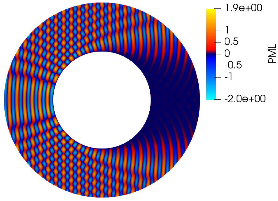
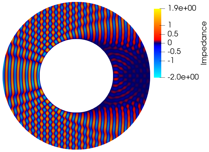
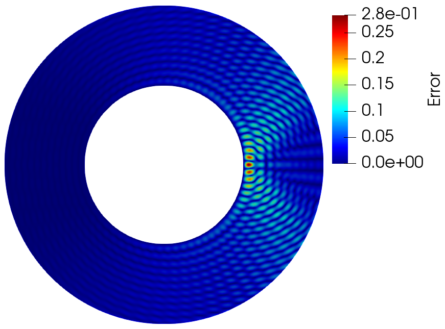
using an element-wise quadrature rule. In the figures we plot the total fields corresponding to and , i.e. and respectively; this is because the total field is easier to interpret than the scattered fields.
Ensuring accuracy of the FEM solutions. The relative errors in the FEM approximations of and are both controllably small, uniformly in , if
| (1.22) |
for some , independent of all parameters, where is the polynomial degree and is the meshwidth. This is proved in [GS23, Theorems 4.9 and 5.3], following earlier results in [DW15, Theorem 5.1 and Corollary 5.2] for the impedance problem with no scatterer and [LW19, Theorem 4.4] for the PML problem with no scatterer and (see also [CFGNT22] for related results). Although , we choose to satisfy (1.22) with . This choice ensures that the FEM error decreases as , and thus the difference between and decreases as . We choose (depending on and ) such that when , (i.e., there are points per wavelength at ). We use triangular elements, and thus there is a variational crime caused by approximating the curved boundaries and ; empirically this error is controlled if is sufficiently small, and thus decreases as under the meshthreshold (1.22). The linear systems are solved using preconditioned GMRES, using the package “ffddm” with tolerance and the preconditioner ORAS (Optimized Restricted Additive Schwarz), as described in [Fre20].
Experiment 1.13 (Scattering by ball, verifying Theorems 1.1/1.7).
We choose , , , and (i.e. the plane wave is incident from the left). Figure 1.1 shows the real parts of the total fields
| (1.23) |
at . We see the error is largest in the shadow of the scatterer near .
Table 1.1 then shows the relative error (defined by (1.21)) for increasing for . The errors in Table 1.1 are constant for fixed as increases, in agreement with Theorems 1.1/1.7. The errors for are roughly 4 to 4.5 times smaller than the errors for , and the errors for are roughly 4 times smaller than the errors for . Since , the factor in the bound (1.14) means that we expect the error for to be 4 times smaller than that for , and the error for to be 4 times smaller than that for , at least when (with the unspecified constant in Theorems 1.1/1.7).
| Relative error for ball | Relative error for ball | Relative error for ball | |
|---|---|---|---|
| 20 | 0.052557755 | 0.012321440 | 0.0035458354 |
| 40 | 0.050360302 | 0.011438903 | 0.0029200006 |
| 80 | 0.050034175 | 0.011050890 | |
| 160 | 0.049001901 |
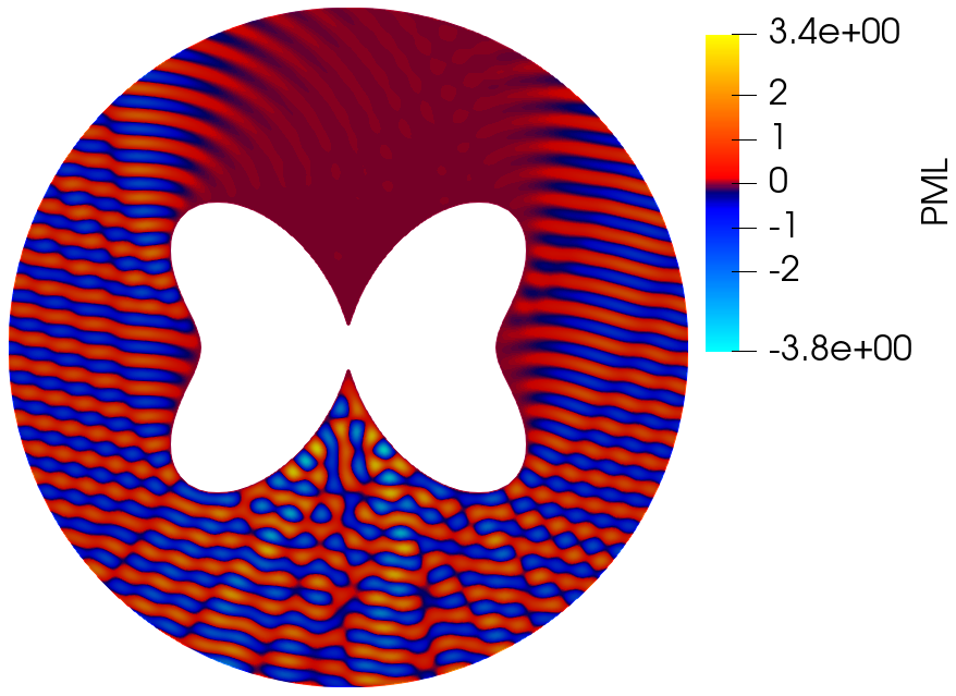
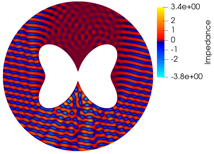
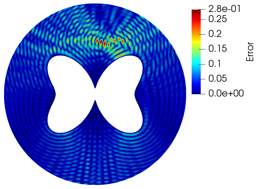
Experiment 1.14 (Scattering by a butterfly-shaped obstacle, verifying Theorems 1.1/1.7).
We choose to be the curve defined in polar coordinates by
, and . We consider the two different incident plane waves corresponding to and .
Figure 1.2 shows the real parts of the total fields (1.23) at with , computed with and . In this case, the error is large in the shadow of the scatterer not only near , but also away from the obstacle. The choice gives a qualitatively similar picture.
Table 1.2 shows the relative error (defined by (1.21)) for this set up for increasing and the two different incident plane waves. For each , the error is constant as increases, again in agreement with Theorems 1.1/1.7. While the errors depend on , the results are consistent with the statement in Theorems 1.1/1.7 that the error can be bounded, from above and below, uniformly in .
| Relative error, incident angle | Relative error, incident angle | |
|---|---|---|
| 20 | 0.066501411 | 0.060746128 |
| 40 | 0.063926342 | 0.061104428 |
| 80 | 0.063212656 | 0.058719452 |
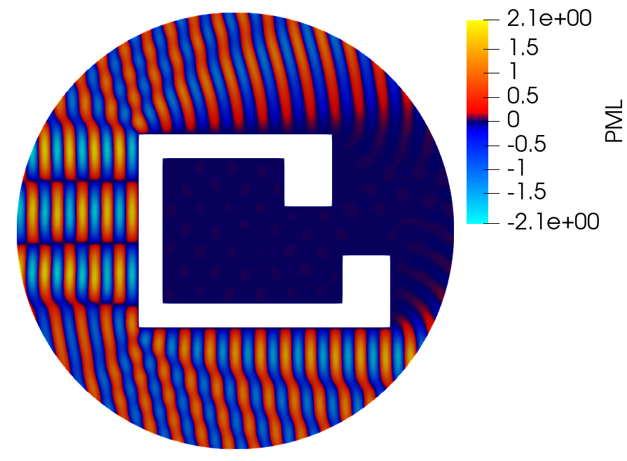
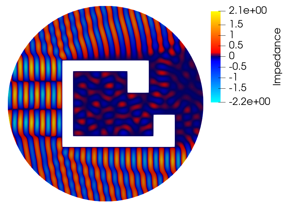
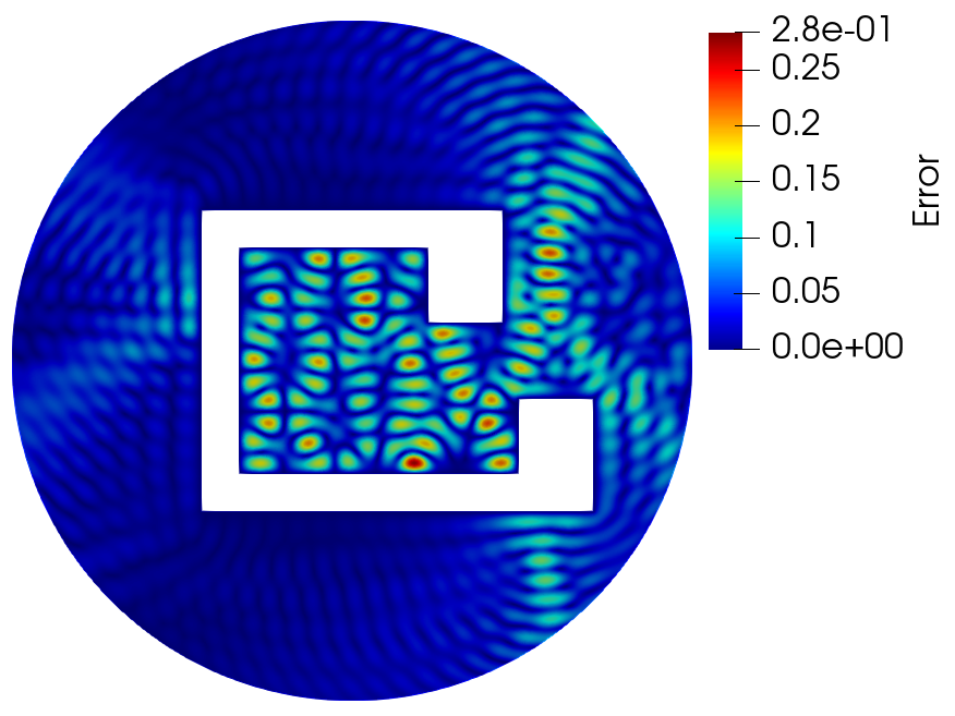
Experiment 1.15 (Trapping created by the impedance boundary).
We choose , , , , and the polygon connecting the points , , , , , , , , , , , The total fields are plotted in Figure 1.3.
This set up is not included in Theorems 1.1/1.7, since is trapping. However we include this experiment to show that artificial reflections from the impedance boundary can excite trapped waves not present in the PML solution (as long as the incident angle is chosen in a careful way depending on , , and the position of ).
Experiment 1.16 (Square , investigating accuracy for increasing with fixed).
Both this experiment and Experiment 1.17 investigate the effect of a non-circular impedance boundary. is the square of side length centred at the origin. We still compute our proxy for using a radial PML, posing the boundary-value problem for on , with the PML region being . Observe that , and so is a fixed distance away from the PML region. We choose , (observe that is then inside – as required), and incident direction . Table 1.3 then shows the relative error for increasing .
When , Table 1.1 showed the error decreasing by roughly a factor of as doubled. In Table 1.3 we see very different behaviour: going from to the error decreases by less than a factor of , and going from to the error does not decrease. Although this experiment is not covered by Theorems 1.2/1.8, since the theorem requires to be smooth, the behaviour of the error is consistent with the main result of Theorems 1.2/1.8, namely that when is not a ball centred at the origin, the relative error is bounded above and below, independent of , as increases.
| Relative error for | Relative error for | Relative error for | |
|---|---|---|---|
| 20 | 0.0832432 | 0.0582767 | 0.0529081 |
| 40 | 0.0802578 | 0.0578435 | 0.0528049 |
| 80 | 0.0772090 |
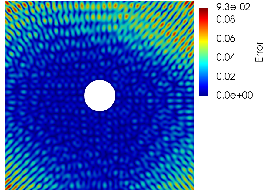
Experiment 1.17 (Square , investigating accuracy for increasing with fixed).
We now investigate the error when is a square as increases with fixed. This situation is not covered by any of Theorems 1.6-1.9. However, we include this experiment since its results, along with those in Experiment 1.16, indicate that the lower bound in Theorems 1.2/1.8 holds uniformly in and .
To investigate the case when increases with fixed, we consider an equivalent problem when is fixed, increases, and the obstacle diameter decreases like . The set up is as in Experiment 1.16 with (so the PML region is ), (so that we need for to be inside ), and the incident direction . Figure 1.4 plots the relative error for this set up with , and Table 1.4 displays the relative error (1.21) for . This set up is equivalent to , , and , and Table 1.4 is labelled with these parameters.
| Relative error | |
|---|---|
| 4 | 0.0593483 |
| 8 | 0.0532721 |
| 16 | 0.0515247 |
1.8. Comparison to the results of [HR87]
Out of the existing results on absorbing boundary conditions in the literature, the closest to those in the present paper are in [HR87]. Indeed, [HR87] used microlocal methods to study the time-domain analogue of the problems (1.1)/(1.6) when (i.e., no obstacle), and proved a bound on the error between the solutions of the analogues of (1.1)/(1.6) at an arbitrary time.
While the results of the present paper also use microlocal methods (using defect measures instead of propagation of singularities used in [HR87]), differences between the results of the present paper and the results of [HR87] are the following.
- •
- •
-
•
[HR87] does not have to deal with glancings rays because it assumes that (i) and (ii) the data is supported away from the artificial boundary. In contrast, (i) we allow the obstacle to be non-empty and have tangent points, and so have to deal with glancing here, and (ii) we allow in (1.11a) to have support up to the boundary (as is needed to use the bound (1.12) in, e.g., the analysis of finite-element methods); therefore a large part of the analysis in §4 takes place at glancing.
1.9. Outline of paper
§2 contains results about semiclassical defect measures of Helmholtz solutions, with these results used in proofs of both the upper and lower bounds in Theorems 1.6-1.11.
§3 proves three results about outgoing solutions of the Helmholtz equation (i.e., solutions satisfying the Sommerfeld radiation condition (1.1c)), Lemmas 3.1, 3.2, and 3.3, with the first used in the proof of the lower bounds, and the last two used in the proof of the upper bounds.
§4 proves Theorem 1.5 (the wellposedness result). Important ingredients for this proof are the trace bounds of Theorem 4.1; since the proofs of these are long and technical, they are postponed to §6.
§5 proves Theorems 1.6-1.11. The upper bounds follow immediately from Theorem 1.5 and Lemma 3.2. However, the lower bounds require showing that there exist rays, created by the incident plane wave, that reflect off and hit at an angle for which the reflection coefficient is not zero. Furthermore, to prove the qualitative bounds Theorems 1.7-1.11 we need to control various properties of these rays explicitly in . §5.3 outlines the ideas used to construct these rays.
Acknowledgements. The authors thank Martin Averseng (University of Bath), Shihua Gong (University of Bath), and Pierre-Henri Tournier (Sorbonne Université, CNRS) for their help in performing the numerical experiments in §1.7. We thank Théophile Chaumont-Frelet (INRIA, Nice) and Ivan Graham (University of Bath) for commenting on an early draft of the introduction; in particular we thank TCF for asking us about the error in subsets of , prompting us to prove the results in §1.6. We also thank the anonymous referee for their constructive comments. EAS and DL were supported by EPSRC grant EP/R005591/1. This research made use of the Balena and Nimpus High Performance Computing (HPC) Services at the University of Bath.
2. Results about defect measures of solutions of the Helmholtz equation
2.1. Restatement of the boundary-value problems in semiclassical notation
While we anticipate the vast majority of “end users” of Theorems 1.6, 1.7, 1.8, and 1.9 will use the Helmholtz equation in the form (1.1) with frequency (and be interested in the limit ), the tools and existing results from semiclassical-analysis that we use to prove these results are more convenient to write using the semiclassical parameter (and the corresponding limit ).
The boundary-value problem (1.1) therefore becomes,
| (2.1a) | ||||
| (2.1b) | ||||
| (2.1c) | ||||
and the boundary-value problem (1.6) becomes,
| (2.2a) | ||||
| (2.2b) | ||||
| (2.2c) | ||||
In the rest of the paper, we use the “-notation” instead of the “-notation”.
Appendix A recaps semiclassical pseudodifferential operators and associated notation.
2.2. The Helmholtz equation posed a Riemannian manifold
While the main results of this paper concern the Helmholtz equation posed in , in the rest of this section (§2), in §4, and in §6, unless specifically indicated otherwise, we consider the Helmholtz equation posed on a Riemannian manifold with smooth boundary and such that there exists a smooth extension of . The reason we do this is that we expect the intermediary results of Theorems 2.15 and 4.1 to be of interest in this manifold setting, independent of their application in proving the main results (Theorems 1.6-1.11). This manifold setting involves the operator , where is the metric Laplacian. Nevertheless, for the reader unfamiliar with this set up, we highlight that can be replaced by , replaced by , and replaced by , and all the statements and proofs remain unchanged.
2.3. The local geometry and the flow
Near the boundary , we use Riemannian/Fermi normal coordinates , in which is given by and is . The conormal and cotangent variables are given by . In these coordinates,
| (2.3) |
where , and are tangential pseudodifferential operators (in sense of §A.3), with of order , and of order with -symbol , with (where the metric in the norm is that induced by the boundary). That is, is the symbol of one plus the tangential Laplacian; in what follows, we often abbreviate to .
The fact that is self adjoint implies that is self adjoint, , and (with the latter two conditions obtained by integration by parts in the variable near ). Let denote the semiclassical principal symbol of , i.e. . In a classical way (see, e.g., [Hör85, §24.2 Page 423]), the cotangent bundle to the boundary is divided in three regions, corresponding to the number of solutions of the second order polynomial equation :
-
•
the elliptic region , where this equation has no solution,
-
•
the hyperbolic region , where it has two distinct solutions
(2.4) -
•
the glancing region , where it has exactly one solution, .
The hyperbolic region plays a crucial role in obtaining the lower bounds in the main results, while we perform analysis near glancing to obtain the upper bounds.
With (i.e., the semiclassical principal symbol of ), the Hamiltonian vector field of is defined for compactly supported by
where denotes the Poisson bracket. Let denote the formal adjoint of , and let denote the generalised bicharacteristic flow in (see [Hör85, §24.3]), defined such that
| (2.5) |
In particular, when and , . By Hamilton’s equations, away from the boundary of , this flow satisfies and , so that it has speed (since ). Recall that the projection of the flow in the spatial variables are the rays.
We now defined some projection maps. Let be defined by . Let be defined by
| (2.6) |
Let and let .
Remark 2.1 (The Dirichlet-to-Neumann map away from glancing in local coordinates).
In the notation above, locally on , the map has semiclassical principal symbol . The minus sign in front of the square root is chosen since, when (i.e. corresponds to a normally-incident wave), the outgoing condition is that (i.e. ), as opposed to (i.e. ).
2.4. Existence and basic properties of defect measures
We first assume that is a solution to
| (2.7) |
where is open with smooth boundary and . When taking traces of , we always do so from rather than from . To define the defect measures associated with we need the following boundedness assumption.
Assumption 2.2.
Given , there exists , and such that for any
Theorem 2.3 (Existence of defect measures).
Reference for the proof.
See [Zwo12, Theorem 5.2]. ∎
Remark 2.4 (The measure ).
The joint measure also describes pairings with the Neumann and Dirichlet traces swapped, since, by (A.2),
We use the notation that for the pairing of a function and a measure. We also use the notation that , where and .
We now recall the following two fundamental results.
Lemma 2.5 (Invariance and support of defect measures).
Let satisfy (2.7) and let be a defect measure of .
(i) In the interior of ,
| (2.9) |
for all ; in particular, if as , then is invariant under the flow.
(ii) is supported in the characteristic set:
| (2.10) |
References for the proof.
2.5. Evolution of defect measures under the flow
Lemma 2.6 (Integration by parts).
Let , , and let . If
| (2.11) |
then, for all ,
| (2.12) |
Corollary 2.7.
Proof of Lemma 2.6.
First recall that is self adjoint, , and ; see §2.3. By integration by parts,
and
Using theses two identities, the expression for (2.3), the self-adjointness of , and the fact that , we obtain that
| (2.14) |
The definition of and the form of in (2.3) imply that
| (2.15) |
Therefore, using (2.14) and (2.15), we have
| (2.16) |
Next, using the definition of , integration by parts, and (2.11), we find that, for any ,
| (2.17) |
Letting , combining (2.16) and (2.17), and using the fact that , we obtain
which is (2.12). ∎
Proof of Corollary 2.7.
Letting in (2.12), using the third equation in (A.2) and the definitions of the measures in Theorem 2.3, we have
| (2.18) |
where , . The idea of the proof is to construct a satisfying the assumptions of Lemma 2.6 with and (and thus ). Since (2.13) is linear in , without loss of generality, we assume that is real. Since and are both smooth, even functions of , abusing notation slightly, we can write
| (2.19) |
Let
| (2.20) |
and
Since and (by (2.3)),
therefore
Since is supported on by (2.10),
| (2.21) |
2.6. Properties of defect measures on the boundary
In this subsection we review the calculations from [Mil00], adapting them to the case when the right-hand side of the PDE is non-zero.
Remark 2.8 (Notation in [Mil00]).
Recall that has defect measure , trace measures , , and , and and have joint defect measure . By [GSW20, Lemma 3.3], is absolutely continuous with respect to , and for some ; hence (2.13) becomes
| (2.22) |
For convenience, we define the differential operator
Lemma 2.9.
There is a distribution on supported in such that
| (2.23) |
where denotes tensor product of distributions. Furthermore, on ,
| (2.24) |
where are positive measures on supported in , and are defined by (2.4).
Proof.
The proof follows [Mil00, Proposition 1.7], replacing at every step by . In particular, by (2.22), is supported in and hence is of the form where each is a distribution on . But, letting with , for and applying (2.22) to , we have for ,
In particular, for , and (2.23) follows.
The result (2.24) about the structure of in the hyperbolic set follows by considering a small neighbourhood in of a point and such that each geodesic trajectory of length centered in intersects the boundary exactly once. We may then use
as coordinates on an open neighbourhood, of . In these coordinates, writing for the pull-back of under , we obtain
In particular, is null for any , and testing by with , and with on , , we have
Now is identically zero on and on . Therefore, for supported in
Similarly, for supported in , . In particular, is a positive distribution on and a negative distribution of , and the result follows. ∎
Next, we decompose into its interior and boundary components, with the following lemma the analogue of [Mil00, Proposition 1.8].
Lemma 2.10.
There is a positive measure on such that
Proof.
Let with and . Then, with , (2.22) implies that
Now,
Therefore, by the dominated convergence theorem,
and, since ,
Since was arbitrary, decomposes as claimed. ∎
The following lemma is the analogue of [Mil00, Lemma 1.9].
Lemma 2.11.
On (i.e. ), and .
Proof.
Let with on and . Let and define . Then, by (2.22) together with the fact that ,
Sending , we obtain
Since was arbitrary, . Replacing by and applying the same argument, we obtain
∎
Next, we prove the analogue of [Mil00, Proposition 1.10]
Lemma 2.12.
On the hyperbolic set ,
(i)
| (2.25) |
(ii) If on some Borel set , then
| (2.26) |
(iii) If
| (2.27) |
on some Borel set for a complex valued function such that is never zero on then
| (2.28) |
where
| (2.29) |
where the superscript “ref” stands for “reflected”. If instead, is never zero, then
Proof.
(i) By combining Lemmas 2.9 and 2.10,
| (2.30) |
Let with on and on . For (so ), let . Since , for and for . Combining (2.30) and (2.22), and using the facts that is even in and for , we find that
By (2.24),
Therefore, by the dominated convergence theorem,
| (2.31) |
Similarly, since is an odd function of , (2.30) and (2.22) imply that
By (2.24),
Therefore, by the dominated convergence theorem,
| (2.32) |
The result (2.25) now follows from solving (2.31) and (2.32) for and .
Lemma 2.13.
In particular, is supported in and does not charge .
Proof.
Lemma 2.14.
Let . Then,
where .
Theorem 2.15.
Suppose that is nowhere tangent to to infinite order. Then, for
| (2.35) |
where denotes the -cotangent bundle to and is defined by (see [GSW20, Section 4.2]).
Proof.
This result is analogous to [GSW20, Lemma 4.8], except that [GSW20, Lemma 4.8] only considers zero Dirichlet boundary conditions, and thus only appears on the right-hand side of [GSW20, Equation 4.3] compared to (2.35) (note that [GSW20] defines the joint measure differently to (2.8), with the result that the signs of are changed here compared to in [GSW20] – compare the definitions [GSW20, Equation 3.1] and (2.8), and then the sign change in the propagation statements [GSW20, Lemma 4.4] and (2.13)).
Examination of the proof of [GSW20, Lemma 4.8] shows that the only time absolute continuity of the measure in that proof is used is in the higher-order glancing set. Therefore, since Lemma 2.14 shows that for some measure that is absolutely continuous with respect to on the glancing set, the result (2.35) follows in exactly the same way as in [GSW20, Equation 4.3 and Lemma 4.8]. ∎
2.7. Linking Lemma 2.12 to concepts in the applied literature
The summary is that in (2.29) is the square of the reflection coefficient describing how plane waves interact with the boundary condition
| (2.36) |
where is a semiclassical pseudodifferential operator. Indeed, when , the boundary condition (2.36) corresponds to the first-order impedance boundary condition at , i.e. (since ). The Helmholtz solution
in the half-plane , corresponds to an incoming plane wave with unit amplitude, and an outgoing plane wave with amplitude . Imposing the boundary condition at , we obtain that
which equals when (since when is flat).
The interpretation of as the reflection coefficient is consistent with the relation in (2.28). Indeed, the defect measure of the solution of (1.6) records where the mass of the solution is concentrated in phase space in the high-frequency limit (see, e.g., the discussion and references in [LSW22, §9.1]). The relation therefore describes how much mass of (since the defect measure is quadratic in ) is reflected from .
The expression for in (2.29) shows that, to minimise reflection from (i.e. to make small), must approximate the symbol of the Dirichlet-to-Neumann map ; recall the discussion in §1.3 and see, e.g. [Ihl98, §3.3.2] for similar discussion in this frequency-domain setting, and, e.g., [EM77b, Pages 631-632], [EM79, Equation 1.12], [Tsy98, §2.2], and [Giv04, §3] for analogous discussion in the time domain.
2.8. Relationship between boundary measures and the measure in the interior
The goal of this subsection is to prove Lemma 2.16 relating the measures and to the measure . We first introduce some notation.
Recall that is defined by (2.6); let
be defined by
| (2.37) |
(i.e., takes a point in and gives it outgoing/incoming normal momentum).
For , let
| (2.38) |
i.e. is the positive time at which the flow starting at from hits again. Similarly, let
i.e. is the negative time at which the flow starting at from hits again.
Given , let be defined by
i.e. is the union of the outgoing flows from points in up to their times and i.e. is the union of the incoming flows from points in up to their (negative) times .
The whole point of these definitions is that in we can work in geodesic coordinates
defined for by (in a similar way to in the proof of Lemma 2.9). Similarly, in we work in geodesic coordinates
In the following lemma, recall that the pushforward measure is defined by .
Lemma 2.16 (Relationship between boundary measures and the measure in the interior).
Proof.
We prove the result for ; the proof for is similar. By Part (i) of Lemma 2.5, is invariant away from the boundary, therefore is invariant on (away from ). Since the flow is generated by in geodesic coordinates, and, in these coordinates, ,
for some . Since ,
and thus, on
| (2.39) |
from which
| (2.40) |
On the other hand, since is in geodesic coordinates, Lemma 2.9 implies that
| (2.41) |
where the factors of arise because .
The following corollary of Lemma 2.16 is an essential ingredient of our proofs of the lower bounds in Theorems 1.6, 1.7, 1.8, 1.10, and 1.11.
Corollary 2.17.
(Relationships between incoming boundary measures, outgoing boundary measures, and measures in the interior.) Let be a solution of (2.7), and let be any defect measure of .
(i) (Between two pieces of the boundary.) Let . Assume that , and that for all . Let
(i.e. is the union of the outgoing flows from points in , projected into ). Then
| (2.42) |
(ii) (Between the boundary and the interior.) Let and . Then
| (2.43) |
and
| (2.44) |
The integrals on the right-hand sides of (2.43) and (2.44) are the shortest times that elements of spend in under, respectively, the outgoing forward flow and the incoming backward flow, with the flows considered until they hit again.
Proof of Corollary 2.17.
(i) The definition of implies that
let denote this set. In , we work in both sets of geodesic coordinates:
as defined above. The coordinates , of satisfy
| (2.45) |
The first equation in (2.45) implies that . By Lemma 2.16, in ,
where the subscripts and show on which neighbourhood of , , , and are considered. This last equality and the second equation in (2.45) imply that
Then
(ii) We prove (2.43); the proof of (2.44) is similar. Using Lemma 2.16 along with the definitions of , , and the geodesic coordinates, we have
where we have used the fact that the point represented in geodesic coordinates by is in iff . Using the change of variables , for , and then Fubini’s theorem, we then have that
as required. ∎
2.9. The reflection coefficient on
To understand how the defect measures of the solution of the truncated problem (1.6) are affected by the artificial boundary , we now show that the hypotheses of Part (iii) of Lemma 2.12 are satisfied, and get expressions for the numerator and denominator in the reflection coefficient in (2.29).
Lemma 2.18.
Corollary 2.19.
Proof of Lemma 2.18.
We prove that
| (2.49) |
and
| (2.50) |
The result then follows from Part (iii) of Lemma 2.12, since (2.49) and (2.50) imply that (2.27) is satisfied.
For , if the traces of have associated defect measures, then, as ,
| (2.51) |
On the other hand, in local coordinates, the boundary condition (2.2c) is
| (2.52) |
so that
| (2.53) |
We now use a similar, but slightly more involved, argument to obtain (2.50). First observe that if is real and the trace of has an associated defect measure , then
| (2.54) |
as , since both and are (see (A.2) and [DZ19, Proposition E.17]). Therefore, (2.54) with and implies that
| (2.55) |
On the other hand by (2.52) and (2.54) (with and ),
| (2.56) |
2.10. The mass produced by the Dirichlet boundary data on
Lemma 2.20.
Suppose that and , then the defect measure of
is given by
where denotes Lebesgue measure on , is the tangential component of the direction at the point , denotes the lowering map given by the metric, and denotes Dirac measure.
Proof.
By using a partition of unity argument, it is sufficient to work locally in a neighbourhood of a point . We work in Euclidean coordinates such that in a neighbourhood of ,
If , then, since ,
and the metric on in the coordinates is
Therefore, since we identify the tangent space of with
Let ; the previous calculation implies that . By change of variable for the semiclassical quantisation (see, e.g., [Zwo12, Theorem 9.3, p. 203],
Observe that for fixed, the phase
is stationary (i.e. ) if and only if
where it is additionally non-degenerate. Consequently, by stationary phase (see, e.g., [Zwo12, §3.5])
The result follows by letting . ∎
3. Properties of outgoing solutions of the Helmholtz equation
The goal of this section is to prove three lemmas (Lemmas 3.1, 3.2, and 3.3), the first two of which concern the solution to the exterior Dirichlet problem:
| (3.1) |
observe that the problem (2.1) is a special case of (3.1) with .
Lemma 3.1.
Suppose that is non-trapping. Then there is such that for all there is such that for solving (3.1)
Lemma 3.2.
The quantity controls, on all rays that are approximately radial, the reflection coefficient as well as the change of the reflection coefficient under the Hamiltonian flow.
Lemma 3.3 (Bounds on ).
If and satisfy Assumption 1.4, then the following hold.
(i) There exists , independent of , such that if , then .
(ii) There exists , independent of , such that if is uniformly in , then .
Regarding Lemma 3.1: this result gives us a lower bound on , and we use this in proving the -explicit lower bounds on the relative error in Theorems 1.7, 1.8, 1.9. The analogue of this result without the explicit dependence of the constant on was proved in [BSW16, Theorem 3.5].
Regarding Lemmas 3.2 and 3.3: the upper bounds in Theorem 1.7 and in Theorem 1.9 follow from applying Theorem 1.5 to and then using these two lemmas.
3.1. Proof of Lemma 3.1
We define the directly-incoming set by
| (3.3) |
where we recall that denotes projection in the variable. The following lemma reflects the fact that is an outgoing solution.
Lemma 3.4.
Proof.
Let be the outgoing resolvent for
i.e., . Fix such that , and let , , with on , . We now extend the Dirichlet boundary data off by letting be the solution of
We now show that can be expressed as an outgoing resolvent plus a function with compact support. To this end, let
and observe that . Since the Dirichlet Laplacian is a black box Hamiltonian in the sense of [DZ19, Chapter 4], by [DZ19, Theorem 4.17], the radiation condition for implies that and hence Now, by, e.g., [DZ19, Theorem 4.4], the range of lies in the range of where denotes the free resolvent. In particular, by the outgoing property of (see e.g. [DZ19, Theorem 3.37])
| (3.4) |
Now, suppose that , where is as in (3.3). Then, for large enough,
and, moreover,
Therefore, by (3.4), Now, since , and
by propagation of singularities (see e.g. [DZ19, Appendix E.4]), .
Now, suppose . Then, and, in particular, there is such that Let
and . Then, , , , and
Observe that
Then consider
In particular, if , .
Next, observe that
so that
In particular,
Taking completes the proof. ∎
Corollary 3.5.
There exists such that, if solves (3.1) and has defect measure , then for any , if with , then, for ,
Proof.
This follows from Lemma 3.4 by observing that, by the definition of defect measures, ; then, if and with , then . ∎
By the definitions of and , another corollary of Lemma 3.4 is the following lemma, originally proved in [Bur02, Proposition 3.5] (see also [GSW20, Lemma 3.4]).
Lemma 3.6.
Suppose that solves (3.1) and has defect measure . Then .
We now prove Lemma 3.1.
Proof of Lemma 3.1.
Suppose that the lemma fails. Then there exist , , such that as and such that
| (3.5) |
Let solve
Since Lemma 3.1 is not used in the proof of Theorem 1.5, the upper bound in this latter result implies that there exists a such that
Let with near and put so that
and , . In particular, by e.g. [GSW20, Theorem 1] there is such that for any with on and , and any small enough,
| (3.6) |
Now, taking the proof is complete for . To see this, observe that using (3.6) with and on
which contradicts (3.5).
Now, for , we can pass to a subsequence in , and assume that has defect measure . By Lemma 3.6, and
3.2. Proof of Lemmas 3.2 and 3.3
In the next lemma, we identify with a subset of .
Lemma 3.7.
Suppose that and Then there is such that
Proof.
First, note that for with supported away from , we can write using the elliptic parametrix construction (Lemma A.2) that there is such that
In particular, by the Sobolev embedding as in [Gal19a, Lemma 5.1] see also [Zwo12, Lemma 7.10],
Therefore, we can assume that
for any . Next, if , then there is with in a neighbourhood of such that
In particular,
Lemma 3.8.
Let be the solution to (3.1). For any , there exists such that, for and small enough (depending on )
| (3.7) |
Proof.
We define . First, observe that it is sufficient to prove that there exists such that, for any and any solving (3.1) having defect measure ,
| (3.8) |
Indeed, if (3.7) fails, then there exists and and such that, for solving (3.1) with and some ,
| (3.9) |
Then, passing to a subsequence, we can assume that has defect measure . Let be arbitrary. Take equal to one in and supported in and supported in and equal to one in . The estimate (3.9) implies
passing to the limit and using e.g. [GSW20, Lemma 4.2] we obtain
which in turn implies, by the support properties of ,
In particular, sending , and using monotonicity of measures
which contradicts (3.8).
We therefore only need to prove (3.8). The definition of defect measures implies , thus, by Lemma 3.4,
Now, invariance of defect measures away from the obstacle combined with the above implies that, for , so that , and ,
By Corollary 3.5, there exist such that
Fix such that . Then, for , we have . Therefore, using the fact that on , we have
| (3.10) |
Now, let and and consider
We claim that ; to see this, suppose that and with and . Then,
and , contradicting (3.10).
Now, since is invariant,
In particular,
Choosing large enough yields (3.8), and the proof is complete. ∎
Proof of Lemma 3.2.
Let be a smooth extension of the normal vector field to , and so that the conclusions of Lemma 3.4 hold, and, , smooth extensions of and . Next, fix such that
and let be smooth, supported in
and equal to one near . By Lemma 3.4, we can find with such that
Now, since is convex, and , . In particular, by Lemma 3.7,
and, using the fact that ,
| (3.11) |
Let
Then, for , the proof is completed, since for any . We now consider the case .
Observe that, by Lemma 3.4,
| (3.12) |
Now, let with on with , and with
with on
and . By (3.12)
where has principal -symbol
| (3.13) |
and thus , and then, by[Zwo12, Theorem 5.1],
However, by the support properties of and and the definition (3.13) of ,
and it follows that, given , there exists such that, for ,
| (3.14) |
On the other hand, by Lemma 3.4,
we obtain in the same way as before, reducing if necessary, that for
| (3.15) |
where is supported in the support of and equal to one on the support of . But, since , has -wavefront set in , thus so does , and it follows that, taking compactly supported near one
| (3.16) | ||||
Hence, by (3.15), for ,
| (3.17) |
Finally, observe that has principal symbol
therefore, using Lemma 3.4 in the same way as before, we obtain
By the support properties of and
Reducing depending on if necessary, we obtain that for
| (3.18) |
Proof of Lemma 3.3.
Proof of (i). First observe that if , then for , . Therefore, on
since , we have
We now claim that
| (3.19) |
where is smooth on . Indeed, the existence of follows from the definition of (1.8) and that on .
Therefore
| (3.20) |
Next, we bound the terms in (3.2) involving the Hamiltonian vector field . First, using again that (where we abuse notation slightly to identify vectors and covectors), we have . Thus, on ,
| (3.21) |
where we have used that is tangent to to write in the last line. Now, by (3.19),
In particular,
| (3.22) |
The required bound on follows by combining (3.20), (3.21), and (3.22).
Proof of (ii). This follows from the fact that and have uniformly bounded norms in . ∎
4. Proof of wellposedness of the truncated problem (Theorem 1.5)
4.1. Trace bounds for higher order boundary conditions
In this section, we consider the solution to
| (4.1) |
where is a Riemannian manifold with smooth boundary such that are the connected components of , and , and have real-valued principal symbols. We further assume that for all ,
| (4.2) |
and for each one of the following holds:
| (4.3) | ||||||
| (4.4) | or | |||||
| (4.5) | ||||||
The first condition in (4.2) ensures non-degeneracy at infinity in (with (4.3), (4.4) and (4.5) the different options for which term in the boundary condition is dominant), and the second condition in (4.2) ensures that the Dirichlet trace is bounded.
Theorem 4.1.
4.1.1. Application of Theorem 4.1 with right hand sides
Corollary 4.2.
Suppose that
| (4.10) |
and either
| (4.11) |
or
| (4.12) |
Then there exists and such that, for , the solution to
with and satisfies
| (4.13) |
Proof.
Let
If , then Theorem 4.1 holds and (4.7) and (4.8) become
| (4.14) |
and
| (4.15) |
respectively. Focusing on (4.14), we therefore impose the conditions that
i.e.,
(observe that this range of is nonempty since , , and ). Choosing , we have
| (4.16) |
where
If , i.e., if (4.11) holds, then the result (4.13) follows from combining (4.16) with (4.15).
4.1.2. Application of Theorem 4.1 to Dirichlet boundary conditions
Corollary 4.3.
There exist and such that if , then the solution of
with and satisfies
4.2. Recap of results of [TH86] about Padé approximants
We now recall results of [TH86] about Padé approximants. These results consider a larger class of approximants than covered in our Assumption 1.4; before stating these results, we explain this difference.
With and defined by (1.8), by Assumption 1.4,
| (4.17) |
As described in §1.3, this choice of and is based on approximating with a rational function in .
The boundary conditions in [TH86] are based on approximating with a rational function in , i.e. [TH86] consider Padé approximants with polynomials and , where the degrees and allowed to be either even or odd. Our polynomials fit into the framework of [TH86] with
| (4.18) |
and then has degree and has degree . For (i.e. when the boundary dimension is ), polynomials with odd powers of do not lead to and being local differential operators, but for (i.e. ) they do, since in this case , i.e., a polynomial in . Our arguments also apply to polynomials with odd powers of in , but we do not analyze them specifically, instead leaving this to the interested reader.
To state the results of [TH86], we let and be polynomials of degree and respectively; this notation is chosen so that, when we specialise the results to our case with (4.18), these and are the same as in Theorem 4.1/Corollary 4.2, i.e., and . Finally, we let
Lemma 4.4.
([TH86, Theorems 2 and 4].) If, and only if, or , then
(a) for , and
(b) the zeros and poles of are real and simple and interlace along the real axis.
Corollary 4.5.
If or , then neither nor has any zeros in .
Proof.
For , this property follows directly from Part (a) of Lemma 4.4. For , this property follows from Parts (a) and (b) of Lemma 4.4; indeed, if there were a zero of (i.e. a pole of ) in , since the zeros of are simple and interlace with the zeros of (by Part (b)), would change sign in , contradicting Part (a). ∎
4.3. Proof of Theorem 1.5
Throughout this section, we let be a smooth family of domains depending on and assume that there is such that
| (4.19) |
Furthermore, we assume that
in the sense that in .
We prove below that Theorem 1.5 is a consequence of the following result, combined with the results from [TH86] in §4.2.
Theorem 4.6.
Let be as in (4.19) and with non-trapping. Let , have real-valued principal symbols and satisfy (4.2) and one of (4.3)-(4.5). Let and satisfy the assumptions of Corollary 4.2, and furthermore let and satisfy
| (4.20) |
Let
satisfy
Then there exists such that for , there is such that for , is well defined and satisfies
| (4.21) |
Proof of Theorem 1.5 using Theorem 4.6.
Theorem 1.5 will follow from Theorem 4.6 (translating between the - and -notations using §2.1) if we can show that the boundary conditions in Assumption 1.4 with either or , with , satisfy
(i) (4.2),
(iii) the assumptions of Corollary 4.2, and
(iv) (4.20),
where and .
Regarding (iii): the first two inequalities in (4.10) are satisfied since , and the third inequality is satisfied both when and when . If , then (4.11) is satisfied, and if then (4.12) is satisfied (since and thus ).
Regarding (ii): if , then (4.4) holds since by definition. If , then (4.5) holds since by definition.
We now prove Theorem 4.6. We first show that, for each and the operator
is Fredholm with ; we do this by checking the conditions of [Hör85, Theorem 20.1.8’, Page 249]. Observe that, for fixed , as a homogeneous pseudodifferential operator, has symbol . Therefore, in Fermi normal coordinates at , we need to check that the map
is bijective, where denotes the solutions to with is bounded on , and
Since ,
and bijectivity follows if the limit on the right-hand side is non-zero. Since and are both real, this is ensured by (4.2) and any of (4.3)-(4.5).
Now, to see that is invertible somewhere, consider . First, note that for the map
is invertible with inverse (see e.g. [Eva98, Chapter 6]). In particular, the Dirichlet to Neumann map
is well defined. Furthermore, is a semiclassical pseudodifferential operator with symbol (see, e.g., [Gal19b, Proposition 4.1.1, Lemma 4.27]). In particular, by (4.2) and (4.3)-(4.5), exists, and hence
Therefore, since for , the operator is invertible, by the analytic Fredholm Theorem (see e.g. [DZ19, Theorem C.8]) the family of operators solving
is a meromorphic family of operators with finite rank poles. To include the Dirichlet boundary values, we observe that by standard elliptic theory, the operator solving
is a meromorphic family of operators with finite rank poles. With with near ,
and thus the operator is well defined.
We start by studying .
Lemma 4.7.
Let and assume that and satisfy the assumptions of Theorem 4.1. Then there exist such that , the solution to
satisfies
Proof.
Suppose the lemma fails. Then there exist with such that ,
Extracting subsequences, we can assume that has defect measure . Moreover, by Corollaries 4.2 and 4.3, we can assume that the trace measures and exist. In particular, since in , . Let denote the billiard flow outside . Then by Lemma 2.12 together with [GSW20, Section 4],
| (4.26) |
Furthermore, using again Corollaries 4.2 and 4.3, we find that
Note also that , , , and satisfy the relations in Lemma 2.12. Next, by Lemma 2.18,
| (4.27) |
Here, we abuse notation slightly, since when , may take the value . In that case, the first equation in (4.27) is replaced by .
Finally, these measures satisfy Theorem 2.15 with which is well defined and satisfies since on .
The proof of Lemma 4.7 is completed by the following lemma.
Lemma 4.8.
Proof of Lemma 4.8.
We consider only the case where . The other case follows from an identical argument but reversing the time direction.
By (4.26), is invariant under away from . We first study the glancing set, . Note that since is convex, where is a boundary defining function for . Note that for , since is convex and , there exist and independent of such that
In particular, since on (by (4.20)), and hence by Theorem 2.15, for ,
Next, we study the case where . Let be the reversed billiard ball map induced by . That is, let be the natural projection map and the inward- and outward-pointing inverse maps. Next, for define
Since is nontrapping, there is such that for all , . In particular every trajectory intersects the boundary in time .
The reversed billiard map is then given by
Since is convex is well defined and, since is invariant under , Then, using (4.27), we have
| (4.28) |
Fix and for , let
We claim that there exist such that for all
| (4.29) |
Once we prove this claim, using (4.28) together with the definition of as the derivative along the flow of , we see that if , then
and hence the proof will be complete.
We now prove (4.29). If the claim fails then there is a sequence
such that
| (4.30) |
Without loss of generality, we can assume that . Note that
By (4.20), since on ,
| (4.31) |
and in particular,
| (4.32) |
Now, let and . We consider the angle between the two vectors
Note that are the tangent vectors to the billiard trajectory just before and after reflection. We define the angle accumulated at , by
As can be seen, e.g., in Figure 4.1,
In particular,
Therefore,
Now, note that if
then
| (4.33) |
for large enough. In particular, (4.30) and (4.33) imply that
which, for large enough, is impossible since . ∎
We now set up our contradiction argument to prove the bound (4.21). Suppose there is no constant such that for all the estimate fails. Then, there exists , , with , , and , such that ,
and such that
Rescaling, we define
Then,
and, with , , ,
where, if a pseudodifferential operator on is given by
then
Putting , we have hence, extracting subsequences if necessary, we can assume that () has a defect measure and by Corollaries 4.2 and 4.3 we can assume that the trace measures for , , , and exist. Moreover, satisfies the relations from Proposition 2.12 where . Finally, extracting even further subsequences, we can assume have defect measures , has defect measure , and the joint measure of and is with
and . Therefore, using e.g. [GSW20, Lemma 4.2] together with Corollaries 4.2 and 4.3 to estimate the norm of by its norm,
Note that each is a finite measure satisfying . Therefore, the sequence is tight and bounded and hence by Prokhorov’s theorem (see, e.g., [Bil99, Theorem 5.1, Page 59] we can assume that for some measure . Moreover, and
| (4.34) |
Lemma 4.9.
The sequences of boundary measures , , and , and are tight.
Proof.
Since is a compact set, we need only consider . By Lemma 2.11,
| (4.35) |
On the other hand, the boundary condition on gives for
Sending , we obtain
In particular,
Now, since and , are real,
Similarly, for
so that, since and are both real,
and hence
which again implies
We now claim that
| (4.36) |
which then implies that is tight. We now show that (4.36) holds in each of the three cases: , and . If , then is compact by (4.5) since by (4.10). If and then is compact by (4.4); observe that the inequality follows from since by (4.10). We now show that if then the first inequality in (4.2) implies that there exists such that if then the intersection (4.36) with (with the constant in (4.3) is empty (and hence compact). Indeed, since and ,
Now, by the first inequality in (4.2)
If then, since , for sufficiently large , and thus (4.36) indeed holds with .
The tightness of and (4.35) then imply that is tight and implies that is tight. Next, the boundary condition on gives that
Hence, and are tight as above. ∎
Since the boundary measures form tight sequences, extracting subsequences if necessary, we can assume , , and for some measures , and , and a complex measure . Furthermore, , and hence . We also have .
Since these measures converge as distributions and in , the equations from Lemma 2.12 and Theorem 2.15 hold for the limiting measures on . (Here, we think of as a graph over .) In addition, since ,
We now introduce notation for various billiard flows in the next section. First, let denote the billiard flow on . Then, define
Note that, the convergence to is uniform and, in the case , agrees with the billiard flow on and we identify the two flows.
Proposition 4.10.
Suppose that and with
Then,
Proof.
Next, we show that is invariant under when .
Lemma 4.11.
Suppose that and that is closed and
Then,
Proof.
First, note that since the convergence of to is uniform,
Therefore, fixing , for large enough,
and
Now, for finite times , is invariant under up to . Combining this with the fact that our assumption on implies that, for large enough, does not intersect in , we have
and
Sending and then , we obtain
as claimed. ∎
Remark.
Note that when , the analogue of Lemma 4.11 is obvious except on the sets and since we can test against away from these sets.
In the case , we use the following lemmas.
Lemma 4.12.
If , then .
Proof.
Fix . Since is nontrapping and , there is and such that
Thus, for large enough
In particular, there is such that for ,
Since , this implies that
and hence, sending ,
Finally, sending proves the claim. ∎
Lemma 4.13.
If then is invariant under away from .
Proof.
Let
Note that is invariant under modulo . Now, . Since , and is nontrapping for ,
Similarly,
Now, for small enough, and , . In particular, for ,
Fix . Then for large enough,
In particular
where in the last line we use that on the relevant set. Similarly, for large enough (depending on ), and
Putting , sending and then , we obtain
and the claim then follows from the fact that
for all ∎
5. Proofs of the bounds on the relative error (Theorems 1.6-1.11)
As discussed in §3, the upper bounds in Theorem 1.7 and in Theorem 1.9 follow from applying Theorem 1.5 to and then using Lemma 3.2. It therefore remains to prove the lower bounds in Theorems 1.6, 1.7, 1.8, 1.10, and 1.11.
5.1. Existence of defect measures
Lemma 5.1.
Proof.
The bound on follows from Lemma 3.1; the bound on follows from Corollary 4.3 and that on follows from the condition (2.1b) that . The bound on follows from Theorem 1.5. The bounds on and follow from Corollary 4.2, and those for from Corollary 4.3. The bound on follows from the condition (2.2b) that . ∎
Remark 5.2 (Neumann boundary conditions).
We do not consider Neumann boundary conditions on because, as far as we know, propagation of measures for Neumann boundary conditions is not available. Indeed, the Neumann boundary condition does not satisfy the uniform Lopatinski–Shapiro condition (see, e.g., [Hör85, Part (ii) of Definition 20.1.1, Page 233]) and, under Neumann boundary conditions, if is normalised so that is bounded, then is typically not uniformly bounded as (for example, when is the boundary of a ball; see, e.g., [Spe14, Equation 3.31]); therefore Assumption 2.2 does not hold.
5.2. Reduction to a lower bound on the measure of the incoming set
Lemma 5.3.
There exists such that if and are sequences of solutions to (2.1) and (2.2), respectively, such that has a defect measure and has defect measure , then
| (5.1) |
and
| (5.2) |
where is the directly-incoming set defined by (3.3).
Proof.
Let be supported in and such that
If is a defect measure of , then by Lemma 3.6. By the definition of defect measures,
and therefore
(where the upper bound on is independent of by [Zwo12, Theorem 5.1]). The bound (5.1) then follows from the upper bound on in Lemma 3.1. The estimate (5.2) is proved in the same way by taking supported in and such that . ∎
Corollary 5.4.
Let , , and be sequences such that satisfies (2.2) with and has defect measure .
(i) To prove Theorem 1.6 it is sufficient to prove that there exists that depends continuously on such that
(ii) Having proved Theorem 1.6, to prove the lower bound in Theorem 1.7 it is sufficient to prove that there exists (independent of ) and such that, for all ,
| (5.3) |
(iii) Having proved Theorem 1.6, to prove Theorem 1.8 it is sufficient to prove that there exists and (independent of ) such that, for all ,
| (5.4) |
(iv) To prove Theorem 1.10 it is sufficient to prove that there exists (independent of ) and such that, for all ,
| (5.5) |
(v) To prove Theorem 1.11 it is sufficient to prove that there exists (independent of ) such that, for all ,
| (5.6) |
Proof.
We prove Part (ii), i.e. the lower bound in (1.14) in Theorem 1.7; the proofs of the other parts are essentially identical and/or simpler.
We first show that it is sufficient to prove that there exists and such that for any , there exists such that, for any direction ,
| (5.7) |
Indeed, having proved (5.7), we let
By Theorem 1.6 and the fact that the constant in this theorem depends continuously on , exists, is , and is independent of . With this definition of , (5.7) implies that the lower bound in (1.14) holds with for , and equal to the respective from Theorem 1.6 for .
We now prove (5.7); seeking a contradiction, suppose that the converse of (5.7) is true; that is, given , for any there exists and sequences , with , such that the solutions and to (2.1) and (2.2) satisfy
| (5.8) |
By extracting subsequences, we can assume that has defect measure and has defect measure by Lemma 5.1
5.3. Outline of the ideas behind rest of the proofs, and the structure of the rest of this section
By Corollary 5.4, we need to prove lower bounds on the measure of the incoming set . We argue by contradiction and assume that is small. The overall plan is the following.
(i) Show that, since is small, mass is created when incoming rays reflect off using Lemma 2.20 above.
(ii) Show that there exists a neighbourhood of rays starting from that hit directly (i.e. without hitting in the meantime) and hit at angles to the normal that are not zero, and not one of the special angles corresponding to the non-zero zeros of (these conditions are made more precise in Condition 5.9 below).
(iii) Propagate the mass created in Point (i) on the rays constructed in Point (ii) using Part (i) of Corollary 2.17 (to go from mass on to mass on ).
(iv) Show that mass is reflected on using the expression for the reflection coefficient in Corollary 2.19 and the fact that the rays hit away from angles where the reflection coefficient vanishes.
(v) Show that this reflected mass produces mass on using Part (ii) of Corollary 2.17 (to go from mass on to mass in ), contradicting the assumption that is small.
For the quantitative (i.e. explicit-in-) bounds the goal is to prove a lower bound on that is explicit in . Therefore, on top of the requirements on the rays in Point (ii) above, we need (a) the angles the rays hit to have certain -dependence (since this will affect the -dependence of the reflection coefficient in Point (iv)), and (b) information about when the reflected rays next hit .
For the bounds on the relative error in subsets of (Theorems 1.10 and 1.11), we also require information about when the rays return to a neighbourhood of , since we need information about the defect-measure mass here (more specifically, ).
Outline of the rest of §5.
§5.4 contains preliminary results required for the ray arguments. §5.5 states the condition the rays must satisfy (Condition 5.9) and results constructing rays satisfying this condition (Lemmas 5.10-5.13). §5.7 proves Lemmas 5.10-5.13. §5.8 bounds the reflection coefficient (2.48) for rays satisfying Condition 5.9. §5.9 proves the qualitative (i.e. not explicit in ) lower bound in Theorem 1.6; the steps (i)-(v) above therefore appear in their simplest form in this proof. §5.10 proves the quantitative (i.e. explicit in ) lower bounds in Theorem 1.7, 1.8, 1.10, 1.11.
5.4. Preliminary results required for the ray arguments
Recall that denotes the -dimensional unit sphere. Given with , let be defined by
The definition of the local coordinates in §2.3 and the fact that imply that
| (5.9) |
i.e., is the reflection of from if is in the illuminated part of and is just if is in the shadow part of .
Definition 5.5.
Given and with , the ray emanating from is the ray starting from .
Definition 5.6.
The ray emanating from is direct if the flow along the ray, starting at , hits before hitting .
We now show that there are direct rays emanating from in every direction.
Lemma 5.7.
Given with . Let denote the set of points of such that both and the ray emanating from is direct. Then,
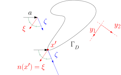
Proof.
We first prove that . Without loss of generality . Let be the point with maximal coordinate. Then by (5.9), by the fact it has maximal coordinate, and so .
We now need to show that, given , . Let be the plane defined by . Choose a cartesian system of coordinates in which , , and is right-handed oriented in . For , let ; i.e. is the reflection of from a boundary with normal . This definition implies that
so that
Hence, there exists such that .
Finally, to show , we need to find such that . Let be a cartesian system of coordinates such that ; see Figure 5.1; let be a point of with maximal coordinate. By definition, , and, since , . Therefore, . Since has maximal coordinate in , the ray emanating from only intersects at , and thus . ∎
The following dilation property is needed for one of the proofs below (the proof of Lemma 5.13).
Lemma 5.8.
Let and let be uniformly convex (i.e. the second fundamental form is positive definite) and such that, for any , . Then, there exists and such that, for any and any , if and , there exists so that
Proof of Lemma 5.8.
Let be an Euclidian system of coordinates in which . Since is included in , there exists and a smooth map such that is given by, in this Euclidian system of coordinates
First observe that, for and
and hence
| (5.10) |
By the definition of (5.9),
| (5.11) |
i.e., is the outward-pointing normal to at .
Given , our plan is to use Taylor’s theorem on to bound below, and then choose appropriately so that this lower bound is . We first record that, since and ,
| (5.12) |
Let be the component of in the direction (i.e., the direction of ), i.e.
| (5.13) |
Then, using (5.11), Taylor’s theorem, (5.13), (5.10), and (5.12), we obtain
| (5.14) |
where
and
where because is uniformly convex.
We now claim that, under the assumption that and , it is always possible to choose so that
| (5.15) |
Indeed, for , the projection of on the hyperplane is a closed hypersurface of (e.g., for it is a closed curve). Since is in the geometrical interior of this hypersurface, for any , there exists satisfying (5.15). For , the projection of on the hyperplane equals two points (one on either side of ); since in this case, there exists satisfying (5.15).
5.5. Statement of the lemmas constructing the rays
Condition 5.9.
Given , there exist , such that, given with , there exists such that
(i) ,
(ii) for all ,
(iii) the emanating rays from hit directly and, for each ray, the angle the ray makes with the normal satisfies
| (5.16) |
(iv) after hitting , the rays travel a distance before hitting either or again.
The in Condition 5.9 are arbitrary angles, but in the proofs below we choose them to be the angles at which the reflection coefficient on (i.e. (2.48)) vanishes, i.e., the angles corresponding to the zeros of in . We set
| (5.17) |
where are defined at the end of §1.3. Then, when for some ,
We now state four lemmas constructing the rays used to prove the different lower bounds on required by Corollary 5.4.
Lemma 5.10 (The rays for general strictly-convex ).
If is strictly convex, then Condition 5.9 holds with for and . Furthermore , are continuous in .
Lemma 5.11 (The rays for ).
If then there exists such that Condition 5.9 holds for all with independent of , and with independent of . Furthermore,
(iv)′ after their first reflection from , all of the rays hit .
Lemma 5.12 (The rays for generic ).
Lemma 5.13 (The rays for when is a smoothed hypercube).
Let coincide with the boundary of the hypercube at distance more than from the corners (as described in the statement of Theorem 1.11).
There exists and (both dependent on but not on ) such that, if and , then Condition 5.9 holds with , , and independent of , and with independent of , and
(iv)′ the emanating rays from hit times, each time with an angle to the normal satisfying (5.16) without hitting in between, and then, after their th reflection, the rays intersect before hitting either or again.
5.6. The ideas used in the proofs of the lemmas constructing the rays
In this subsection, we outline the ideas used in the proofs of Lemmas 5.10-5.12, in the simplest possible case when (i.e., the boundary condition on is the impedance boundary condition (1.10)). In this case and there are no non-zero angles ; when such angles exist, mass needs to be excluded in a careful way from the neighbourhoods described below so that the rays avoid these angles. The proof of Lemma 5.13 has a different character to the proofs of Lemmas 5.10-5.12, and so we postpone discussion of the ideas of that proof until the start of the proof itself.
The idea behind the ray construction for general strictly-convex in Lemma 5.10 is as follows. We consider a point in that is the extremum point on in the direction of . The rays emanating from a neighbourhood of this point are rays in the direction , and thus hit directly. Since is strictly-convex, these rays cannot be normal to at more than one point, see Figure 5.2, and thus the required neighbourhood exists.
For the proof of Lemma 5.11, we need in addition to quantify how far from the normal the ray described in the last paragraph hits . When , we show that a set of points of volume can reach with an angle ; see Figure 5.3.
For the proof of Lemma 5.12, i.e. when is not a sphere centred at zero, we recall from Lemma 5.7 that, given any direction, there exists a direct ray emanating from in that direction. We need to show that at least one of these rays hits non-normally. Since is not a sphere centred at the origin, there exists with . We use Lemma 5.7 to identify a point such that the ray emanating from is in the direction and does not hit again. In the limit , the rescaled obstacle shrinks to the origin; therefore the rays emanating from a neighbourhood of hit with an angle close to the angle between and ; this angle is , with independent of ; see Figure 5.4.
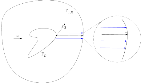
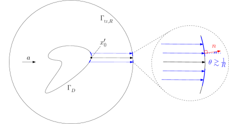
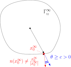
5.7. Proofs of Lemmas 5.10-5.13
In the proofs of these lemmas we use the notation that is the angle between vectors and ; i.e.
where the range of is .
Proof of Lemma 5.10.
Step 1. Construction of direct emanating rays in the direction of .
Without loss of generality, we assume that . Let be the point on with maximal coordinate. By translating the obstacle , we can assume that . Then, locally near , for any , where is small enough
| (5.18) |
where and , and . Moreover, for small enough and
| (5.19) |
Indeed, if not then there exist , such that . But then, extracting subsequences if necessary, and . In particular, by maximality of the coordinate at , . But, near (5.18) holds and in particular, for large enough, , which is a contradiction.
Observe that, shrinking if necessary, is outward-pointing along , and
| (5.20) |
where depends only on and hence . By (5.9), for all , and thus the rays emanating from are the rays in the direction; see Figure 5.2. By (5.19), these rays hit before hitting again. The neighbourhood will be a subset of , and thus Point (ii) in Condition 5.9 follows.
Step 2. Parametrisation of .
Let be such that
since is strictly convex, this property holds without needing to reduce and thus still only depends on . The outward-pointing normal to is given by
For , let be the angle between the ray emanating from and the normal to ; since ,
| (5.21) |
We use later the facts, obtained from from (5.21) by direct calculation, that,
| (5.22) |
and, in ,
| (5.23) |
We also use the following quantities,
| (5.24) |
Step 3. Avoiding the angle .
Recall that our goal is to construct so that
where and depend only on . Our plan is to exclude mass from for each , taking care that the volume is still bounded below to give Point (i) of Condition 5.9.
Avoiding the angle zero corresponds to obtaining a lower bound on . By Taylor’s theorem,
where is defined by (5.24), and depends only on . By the definition of in (5.24),
Suppose that . Then
On the other hand, if , then
Therefore, in both cases, if , then there exists a set with
| (5.25) |
such that
Therefore, for , by (5.21)
and we conclude that
| (5.26) |
Step 4. Avoiding the angles .
Given , let be such that
| (5.27) |
i.e., is the point in where is closest to . Let
| (5.28) |
In the following we use the notation for the line segment between and , i.e.
and denotes the Euclidean inner product on .
The main idea of the rest of this step is the following: is, by definition, smallest at , and will be smallest when the minimum in (5.28) is attained, i.e. ; in this case, the idea is for the size of the neighbourhood of that we exclude to be dictated by using Taylor’s theorem
| (5.29) |
where the requirement that the right-hand side is bounded below determines the size of the excluded neighbourhood. The issues we then have to deal with are (a) is not necessarily equal to , and (b) is zero when , and then the second-order term in (5.29) blows up.
To deal with Point (b), we first consider points in where the second-order term in (5.29) does not blow up. Let
| (5.30) |
where will be chosen later in the proof (when dealing with the points not in ). By (5.22), for any , for . Recalling the definitions (5.24), and using (5.29) and (5.23), we have
| (5.31) |
where
| (5.32) |
and the unit vector is defined by
| (5.33) |
Let
where ; then (5.31) implies that
We now deal with Point (a) above (i.e. that is not necessarily equal to ). If , for to be fixed later, then, by (5.27),
| (5.34) |
If , then
and then
| (5.35) |
Combining (5.34) and (5.35), we have
| (5.36) |
recall that we still have the freedom to choose and .
We now deal with the case ; the idea here is the following: consists of points such that every point on has , i.e. bounded below. If , and we chose appropriately, then can be small compared to , and thus . can be bounded below. Indeed, let ; if , then
| (5.37) |
We now need to consider with . The sequence of ideas here is that (i) by the definition of , there is a point, , in with , (ii) the argument in (5.37) applies at , (iii) , which is small, (iv) can be chosen so that on and then can also be made small. The detail is as follows: let
the set on the right-hand side is not empty by (5.22) and the definition of (5.30). Let . This definition implies that for . Therefore, using the mean-value theorem and (5.23), we have
Using this together with (5.37), we obtain
| (5.38) |
Collecting both cases (5.37) and (5.38), we obtain that
| (5.39) |
We now tune and to make the volume of big enough, and conclude the step by selecting suitable and . From the definition (5.40),
| (5.42) |
where
Observe that is the complement of a double cone, rotationally symmetric around the axis (recall that defined by (5.33) depends on and not ); therefore, decreases as . By integrating in hyperspherical coordinates centered at with axis , and comparing to , we have
Using this in (5.42), we have
| (5.43) |
We now fix both and to be sufficiently small such that
then (5.43) implies that
| (5.44) |
To conclude this step, we now restrict so that and then set ; then (5.41) implies that if
| (5.45) |
then
| (5.46) |
Step 5. Conclusion.
Combining the result of Step 3 (5.26) and the result of Step 4 (5.45)-(5.46), we see that if
then
We then let
| (5.47) |
so that
Points (i) and (iii) in Condition 5.9 then hold with
| (5.48) |
and
| (5.49) |
Since and (defined by (5.24) and (5.32)) all depend continuously on , and depends continuously on , and depend continuously on . The constant depends on , , and , and thus also depends continuously on . ∎
Before proving Lemma 5.11, we prove the following simple lemma.
Lemma 5.14.
If , then the emanating rays from hit directly with an angle to the normal satisfying .
Proof.
Since , any ray starting from hits with an angle to the normal satisfying . Since , the result follows. ∎
Proof of Lemma 5.11.
We first observe that Point (iv)′ follows from the same argument used to prove Lemma 5.14; this implies that with independent of .
The fact that is independent of follows from the proof of Lemma 5.10; see (5.20). By direct calculation from the definitions (5.24), (5.32)), using the fact that where is a constant, we obtain that
Using these asymptotics in (5.47), (5.48), and (5.49), we find that is independent of and (observe that the first minimum in (5.49) and the second minimum ).
Remark 5.15 (Lemma 5.11 when ).
Recall that when , then , inspecting the proof of Lemma 5.11, we see that the result then holds with and .
Proof of Lemma 5.12.
For , let and
We now claim that there exists such that is non-empty. Indeed, first observe that the map
is continuous. The only way for this map to be constant is for to be a sphere centred at the origin, and this is ruled out by assumption. Since in , is Lipschitz, and the set has full dimensional (i.e. surface) measure. Therefore, the image of the map contains an interval, and the claim follows. We note for later that is open in .
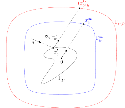
Let . By Lemma 5.7, there exists such that
see Figure 5.5. For , let denote the point where the ray emanating from first hits ; we use later the fact that this definition implies that
| (5.50) |
The neighbourhood in Condition 5.9 will be for sufficiently small, independent of , and this ensures that Point (i) holds with independent of . Let be small enough so that ; this ensures that Point (ii) holds with independent of .
We now show that Point (iii) of Condition 5.9 holds with and independent of . Let be defined by
| (5.51) |
this limit exists is the limit of subsets of and as . We claim that it is sufficient to prove that for sufficiently small (independent of ). This shows the analogue of Point (iii) in Condition 5.9 with replaced by ; i.e., that the emanating rays from points in hit directly with an angle to the normal satisfying (5.16) with and independent of . Point (iii) for with sufficiently large then follows since is the limit of subsets of , and as .
We now claim that to prove that for sufficiently small (independent of ) it is sufficient to show that for all . Indeed, if this is the case then . Then, since (i) is open in and contains , and (ii) for , there exists such that for all .
We now show that for all . We do this by showing that for a sequence , and then the result follows from (5.51). Observe that the inclusions (1.18) imply that , for any , and thus is bounded as . Therefore, there exists a sequence and a such that , and thus also
| (5.52) |
By simple geometry, as ,
by (5.50). Comparing this to (5.52), and using the uniqueness of the limit, we see that . Since is convex, and thus star-shaped, , and the proof that for all is complete; this completes the proof that Point (iii) of Condition 5.9 holds with and independent of .
Finally, we show that Point (iv) of Condition 5.9 holds for sufficiently large with with independent of . Since and satisfies the inclusions (1.18), after hitting , a ray must travel a distance before hitting . Therefore, we only need to show that, after hitting , a ray must travel a distance before hitting again. Since tends to a limit as , this result follows if the rays first hit with angle to the normal satisfying , with independent of , which is the case because and satisfies the inclusions (1.18). ∎
Proof of Lemma 5.13.
The overall plan is to select a ray emanating from that returns to after multiple reflections from the sides of the hypercube . We do this by identifying with by reflection through the lines
(where denotes the th component of the vector ); under this identification the corners of the hypercube correspond to the points . Since coincides with the boundary of the hypercube only at distance more than from the corners, we need to make sure that the selected ray avoids these neighbourhoods of the corners; hence the requirement that in the statement of the result. We highlight that the constant in the bound then depends only on the dynamics of the rays, and hence is independent of .
Step 0: Preliminary notation and results. This argument involves three domains, and three associated flows. The first domain is , with associated generalised bicharacteristic flow (as defined in §2.3). The second domain is , and we denote the generalised bicharacteristic flow on by . The third domain is the hypercube , and we denote the generalised bicharacteristic flow on by .
By the definition (5.9) of , if both and are in the illuminated part of (i.e., ), then there exists (depending on the Lipschitz constant of ) such that
| (5.53) |
i.e. is Lipschitz.
We record for later use that, since and ,
| (5.54) |
Finally, let be a non-empty, uniformly-convex open subset of in which (such a exists, since Lemma 5.7 implies that is not everywhere flat). Shrinking if necessary, we can assume that
| (5.55) |
this implies that the first assumption of Lemma 5.8 holds with . The neighbourhood we construct will be a subset of .
Step 1: Bounding the distance between projections of the flow on .
For , , since ,
| (5.56) |
We now show that the same inequality holds for the flow on ; i.e., that for , ,
| (5.57) |
To prove (5.57), we compare with by using the relationship between the two flows and .
First, observe that, since
we can assume that
Therefore, there exists and such that
| (5.58) |
i.e., after time , the free-space rays from and are either in the same hypercube or in adjacent hypercubes. We use the following notation for the components of , :
| (5.59) |
Now, observe that by (5.58) and the relationship between and ,
| (5.60) |
where
Let . We first assume that ; then
| (5.61) |
Since , , , and hence . Now, because ,
| (5.62) |
Similarly, since ,
| (5.63) |
Then, combining (5.61), (5.62), and (5.63), we have that, for with ,
| (5.64) |
If , the prove of (5.64) follows in a very similar way; if , it is straightforward to check that (5.64) holds with equality. Hence (5.64) holds for any . Recalling the notation (5.59), we therefore obtain from (5.60) and (5.64) that
Step 2: Selecting a periodic ray. Let be the finite set of unit vectors forming an angle belonging to to one of the elements , where denote the unit vectors in cartesian coordinates. With as in Step 0, contains a non-empty open subset of by Lemma 5.7, and therefore contains a vector of the form
(since vectors of this form are dense in ). Let be such that .
We identify with as described above. Then, given any ,
| (5.65) |
the factor of two is because one reflection changes the parity.
The trajectory starting from and evolving according to the flow can be identified with the trajectory in
therefore, by (5.65), the former trajectory is periodic, with period at most . Thus there exists such that ; let be the infimum of such s. Therefore
| (5.66) |
and
| (5.67) |
Since , the flows and acting on agree up to (at least) time ; i.e.
| (5.68) |
Furthermore, since , the flows and acting on never hit at an angle belonging to .
Finally, observe that a length of a ray can be reflected at most twice. Therefore, since the length of for is at most , if , then the number of reflections of this ray for , , is bounded by , i.e.,
| (5.69) |
Step 3: The neighbourhood on . The neighbourhood is chosen later in the proof as a subset of
| (5.70) |
where (independent of ) is small enough so that, for all ,
| (5.71) |
Since the neighbourhood will be a subset of , the second condition in (5.71) implies that Part (ii) of Condition 5.9 holds with , which is positive since , and the third condition in (5.71) implies that Part (iii) of Condition 5.9 holds with .
By (5.57), the fact that , (5.53), and (5.66), we have, for any and any
| (5.72) |
Therefore, if , then
| (5.73) |
for all and for all . Combining (5.73), (5.67), and (5.68), we have
| (5.74) |
and
| (5.75) |
Step 4: Avoiding the corners. Under the identification of with , the corners of the hypersquare correspond to . Given , each point on the ray for has a corner that is closest; we let denote the subset of these corners that are a distance away. More precisely,
We then order the elements of with the closest first; i.e., with non-decreasing with .
We now prove that if , then
| (5.76) |
To prove this, observe that, for , by (5.66) and (5.53) (in a similar way to as in (5.72)),
if . Therefore, if , the distance between the rays is . If then, since , is at most distance away from a point on the ray , and thus .
It turns out that we will not need to restrict further in the proof; we therefore set
| (5.77) |
and observe that this satisfies the requirements imposed on earlier in the proof (to ensure that (5.73) and (5.76) hold).
We now select one set of corners to work with for all . Let . By (5.76),
so that
| (5.78) |
Furthermore, since , the number of corners within distance of the ray is less than or equal to the number of reflections, i.e.,
| (5.79) |
We now iteratively construct , , such that the ray for is at least a distance from where , , are defined below (see (5.86)) and, in particular, have the property that . Given , if , we set . Otherwise, first observe that, for ,
| (5.80) |
by (5.54) and the fact that ; we can therefore restrict attention to . Let , to be fixed later. We first assume that there exists so that, with the constant associated to by Lemma 5.8,
| (5.81) |
we later use Lemma 5.8 to show that such an exists once the value of has been fixed. By, respectively, the triangle inequality, the convexity of , (5.81), and the fact that we’re dealing with the case that , we have that, for ,
| (5.82) |
Having bounded the distance from the ray to , we now bound the distance to for . By, respectively, the triangle inequality, (5.53), and (5.66), for and ,
| (5.83) |
The two inequalities (5.82) and (5.83) imply that if and satisfy
| (5.84) |
and is defined by
| (5.85) |
then
and
This last two inequalities, combined with (5.80), imply that
as required. We observe for use later that (5.84) implies that
| (5.86) |
Since the value of has been fixed by (5.85), it remains to show that there exists satisfying (5.81). We now use the freedom we have in choosing to ensure that the can use Lemma 5.8 to construct such an . Recall that we chose so that the assumptions of Lemma 5.8 hold; let be the associated constant. We impose the condition that
| (5.87) |
where we have used the definitions of (5.85) and (5.86) and the fact that . Observe that (5.87) is a condition that is sufficiently small (recall that has been fixed by (5.77)).
The rationale behind imposing (5.87) is as follows; recalling the definition of (5.70), we see that implies that for . The first inequality in (5.87) implies that , for all , and, since (by (5.71)),
These relations combined with (5.55) imply that the assumptions of Lemma 5.8 are satisfied with . This lemma therefore implies that there exists satisfying (5.81), for all .
In summary, we have proved that the ray , , is a distance at least from any of the corners , and a distance at least from any of the other corners by (5.78).
Let be defined by the second equation in (5.86) with and with fixed to satisfy (5.87). By (5.79) and (5.69), so that . Therefore, with
the ray , is a distance at least from any corner. By (5.86) and (5.87), (and hence ) depends on , , , and , and hence only on .
Step 5: Putting everything together. By combining the results of Step 4 with the results (5.74) and (5.75) of Step 3, we have
| (5.88) |
We now define the neighbourhood (the neighbourhood of rays in the statement of the lemma) as a neighbourhood of . Indeed, we let
with chosen sufficiently small; if is independent of , then this implies that for some independent of ; i.e., that Point (i) of Condition 5.9 holds.
We first choose sufficiently small so that ; since (5.77) is independent of , can be chosen to be independent of . As discussed below (5.71), the inclusion ensures that Points (ii) and (iii) of Condition 5.9 hold.
Point (iv) in the statement of the result will follow if we can show that, for all ,
| (5.89) |
Indeed, the second property in (5.89) (missing the corners) implies that all three flows are the same when applied to for , i.e.
5.8. Bounding below the reflection coefficient (2.48) for rays satisfying Condition 5.9
In the follow result, we use the subscripts and on to denote the hyperbolic set on and , respectively.
Lemma 5.16 (Lower bound on the reflection coefficient for general ).
Let . Given , let
| (5.90) |
observe that is well-defined since on .
We make three remarks.
-
•
The rationale behind the definition of (5.90) is that later we apply it to sets whose elements are of the form where (so that ). In this case, is the angle the vector makes with the normal to .
-
•
We have denoted the constants in (5.91) by and since we later apply this lemma with and .
-
•
We highlight that only depends on and , and not on .
5.9. Proof of Theorem 1.6 (the qualitative lower bound)
Similar to above, we use the subscripts and on (and subsets of it) to denote the hyperbolic set on and , respectively; we use analogous notation for boundary measures.
Proof of Theorem 1.6.
By Part (i) of Corollary 5.4, we only need to show that . We now follow the steps outlined in §5.3; seeking a contradiction, we assume that . The inequality (2.44) from Point (ii) of Corollary 2.17 implies that . Therefore (2.26) implies that
and Lemma 2.20 therefore gives that
| (5.95) |
Given and , let be defined by (5.17); i.e., is the set of non-zero angles at which the reflection coefficient (2.48) vanishes. Let the set be given by Lemma 5.10; i.e., the rays emanating from are non-tangent to and hit directly and at angles bounded away from . Let
By (5.95), . Therefore, using the equality (2.42) from Point (i) of Corollary 2.17 and the fact that on ,
| (5.96) |
where
where and are defined in (2.38) and (2.37) respectively, and equals restricted to ; observe that since is (strictly) convex.
5.10. Proof of the lower bounds in Theorem 1.7, Theorem 1.8, Theorem 1.9, Theorem 1.10, and Theorem 1.11
Recall from Corollary 5.4 that to prove the lower bounds in Theorems 1.7, 1.8, 1.10, and 1.11, we only need to bound and below; the following lemma provides the necessary lower bounds.
Lemma 5.17.
Suppose Condition 5.9 holds for with independent of and with independent of . Then, there exists such that, for all ,
(i)
| (5.97) |
(ii) If, in addition, there exists such that, for the interior billiard flow in , these rays are reflected on times, without being reflected on in between, and after their th reflection all of these rays intersect without being reflected before, then
| (5.98) |
Proof of (i). As in the proof of Theorem 1.6, we argue by contradiction and follow the steps in §5.3. Suppose that Condition 5.9 holds for , but, for any , there exists such that
| (5.99) |
Let
| (5.100) |
We now claim that
| (5.101) |
Indeed, Part (ii) of Corollary 2.17 implies that
and then to prove (5.101) we only need to show that
| (5.102) |
Let . Then, since and , if ,
and then (5.102) follows for . On the other hand, if , then
and then (5.102) follows for .
We now use Lemmas 2.12 and 2.20 to obtain a lower bound on . The two equations in (2.25) imply that
| (5.104) |
(see (2.32)). By Lemma 2.20 and Part (i) of Condition 5.9,
| (5.105) |
By the assumption that Condition 5.9 holds (with independent of ), on . By the definitions of (5.100) and (1.7), for and thus on . Combining (5.104) with (5.105) and (5.103), and using the facts that is nonnegative and , we have
If
| (5.106) |
(observe that, since is assumed independent of , this upper bound on is independent of ), then
We now use Corollary 2.17 to propagate this lower bound on to a lower bound on . Indeed, Part (i) of Corollary 2.17 then implies that
| (5.107) |
where
where and are defined in (2.38) and (2.37) respectively, and equals restricted to .
Finally, using Part (ii) of Corollary 2.17 with Point (iv) of Condition 5.9, and then using (5.108) and (5.107), we have,
| (5.109) |
We now restrict so that, in addition to satisfying (5.106), satisfies
(observe that, since and are assumed independent of , this upper bound is independent of ). Thus can be chosen sufficiently small (independent of ) such that (5.109) contradicts (5.99), which is the desired contradiction.
Proof of (ii).
If the assumption of (ii) holds, then our contradiction argument also assumes that for all there exists such that
| (5.110) |
Applying Part (i) of Corollary 2.17 more times and using (5.108), we construct , satisfying
| (5.111) |
and so that for any , intersects before hitting or . Therefore, by (5.111) and (5.107)
| (5.112) |
Finally, since any ray entering spends a time at least in this annulus, Part (ii) of Corollary 2.17 implies that
| (5.113) |
where we have used (5.112). Therefore, if
then (5.113) contradicts (5.110), which is the desired contradiction. (Observe that, similar to in Part (i), the upper bound on is independent of since and are independent of .) ∎
Proof of the lower bounds in Theorems 1.7, 1.8, 1.10, and 1.11.
The lower bounds will follow from combining Corollary 5.4, Lemma 5.17, and the ray constructions in Lemmas 5.10-5.13.
For Theorem 1.8 (for generic ), Lemma 5.12 implies that the assumptions of Part (i) of Lemma 5.17 are satisfied with independent of , and sufficiently large; the required lower bound (5.4) on then follows by inserting this (lack of) -dependence into (5.97).
For the lower bound in Theorem 1.7 (for ), Lemma 5.11 implies that the assumptions of Part (i) of Lemma 5.17 are satisfied with independent of , with independent of , and sufficiently large. The required lower bound (5.3) then follows by inserting these -dependences into (5.97), and observing that, for sufficiently large,
| (5.114) |
For Theorem 1.10 (i.e. the local error for ), Point (iv)′ in Lemma 5.11 implies that the assumptions of Part (ii) of Lemma 5.17 are satisfied and sufficiently large. The required lower bound on (5.5) then follows from (5.98) using (5.114) and the fact that is independent of . The fact that the result holds with when follows from Remark 5.15.
6. Proof of the trace bounds (Theorem 4.1)
6.1. Strategy of the proof
To illustrate some of the main ideas, consider the BVP (4.1) with , compact, and the boundary condition imposed on the whole of , i.e.,
| (6.1) |
In the notation of Theorem 4.1, we have , and the bounds (4.7) and (4.8) in the case are that
| (6.2) |
and
| (6.3) |
We now show how to obtain these bounds; pairing the PDE in (6.1) with and integrating by parts, we have
| (6.4) |
Taking the imaginary part of (6.4), we find that
| (6.5) |
Taking the real part of (6.4) and adding to both sides of the resulting equation, we find that
| (6.6) |
Combining the inequality (6.5) with the boundary condition in (6.1), we obtain the first result (6.2). Then, using (6.5) in (6.6), we obtain the second result (6.3).
The proof of Theorem 4.1 follows similar steps; indeed, the two main ingredients are (i) bounds on the traces in terms of the data and norms of , and (ii) a bound the norm of in term of the traces and the data. The bound in (ii) is obtained by considering and integrating by parts, similar to above, with the inequality (6.19) the generalisation of the inequality (6.6). The bounds in (i) are obtained by considering , similar to above, but also (with Lemma 2.6 above considering a general commutator, and Lemma 6.1 specialising to the case of a normal derivative).
The additional complications for the bounds in (i) are because we need to consider the cases where and are both elliptic (Lemma 6.2), where is small and elliptic (Lemma 6.3), and where is elliptic and small (Lemma 6.4), These three cases are considered in §6.2, and then in §6.3 we show that, under the assumptions (4.3)-(4.5), the bounds in these three cases cover all of .
6.2. A priori estimates
We begin by proving some a-priori estimates for (4.1). As usual, we work near where is locally given by , as in §2.3. We repeatedly use the integration by parts result in Lemma 2.6.
Lemma 6.1.
If solves (4.1), then, for all and for all ,
Proof.
Remark.
We now show a bound where and are both elliptic.
Lemma 6.2.
Suppose that . Then for any with
there exist and such that for any , ,
Proof.
Let self-adjoint with . Let with
We can assume without loss of generality that is microlocally the identity in a neighbourhood of . Next, let and and denote microlocal inverses for and on . Then, by Lemma 2.6,
First, note that
where
In particular, by the standard elliptic parametrix construction, for all ,
Therefore,
Now, using (4.1),
and
In particular, letting with ,
Now, choose self adjoint (i.e. ) such that is elliptic on . Then, since and have real-valued symbols and is elliptic on ,
and
| (6.8) | ||||
We now consider small and elliptic:
Lemma 6.3.
Let . Then for all there is and such that for all , with
| (6.9) |
and with
there is small enough such that for all and
| (6.10) | ||||
Moreover, if (6.10) holds with
Proof.
Throughout the proof, we take self-adjoint with if and otherwise. We assume that
As in Lemma 6.1, let with on . Let
| (6.11) |
Then (2.11) holds, and satisfies the assumption of Lemma 2.6; since , (2.12) implies that (6.7) holds.
Since is elliptic on , there exists a microlocal inverse for on ; that is, for any with ,
| (6.12) |
and hence, using the fact that we are working with compactly microlocalized operators on to see that all norms are equivalent up to remainders, we have
| (6.13) | ||||
Now, observe that
where
In particular, using the elliptic parametrix construction as before, we have
| (6.14) | ||||
If , we assume that . Therefore, for all
for our choice of . Next, since is elliptic on , for any compact, there exists small enough such that
Moreover, if , then there is small enough such that
In particular, since is real-valued, there is self adjoint, elliptic on , such that
In particular, then the sharp Gårding inequality [Zwo12, Theorem 9.11] gives
and we obtain from (6.14),
Next, we write, as above,
to obtain
and this finishes the proof. ∎
Finally, we consider the case elliptic and small.
Lemma 6.4.
For all , there is and such that for all , with
| (6.15) |
and with
there is small enough such that have for and ,
| (6.16) | ||||
Moreover, if , then (6.16) holds with .
Proof.
Throughout the proof, we take self-adjoint with if and otherwise. We assume that
Let and be defined by (6.11).
Since is elliptic on , there exists a microlocal inverse for on ; that is, for any with ,
| (6.17) |
Arguing as in the proof of Lemma 6.3, we obtain the analogue of (6.14) with , namely
If , we assume that . Therefore, for all
for our choice of . Now, any compact, there is small enough such that
Moreover, if , then there is small enough such that
Therefore, choosing with non-negative symbol such that is elliptic on , we have
In particular,
Therefore,
Then, using (6.17) again the second claim follows. ∎
6.3. Proof of Theorem 4.1
Throughout this section we assume that (4.2) holds. In particular, the union of the elliptic sets for and covers and is elliptic on .
Proof.
We start by briefly considering the conditions (4.3)– (4.5) separately. Suppose first that (4.3) holds. Then, fixing , such that Lemmas 6.3 and 6.4 with hold, there exist satisfying (6.9) and satisfying (6.15) (both with ) such that
Next, if (4.4) holds, there exists such that
Fixing , such that Lemma 6.3 holds with and 6.4 holds with , there exist satisfying (6.9) with and satisfying (6.15) with such that
Finally, if (4.5) holds, there exists such that
Fixing , such that Lemma 6.3 holds with and 6.4 holds with , there exist satisfying (6.9) with and satisfying (6.15) with such that
In particular, in all cases, there exist , such that for , the estimates of Lemma 6.3 hold for , those for (6.4) hold for , and those of Lemma 6.2 hold for such that
Finally, using Lemma 6.2,
Since
we have all together
| (6.18) | ||||
Finally, observe that
Letting with elliptic on and elliptic on , we have
Therefore, for any ,
| (6.19) |
Using this in (6.18) and taking
| (6.20) |
we obtain
Shrinking such that and taking small enough such that , the proof is complete since the inequality (4.6) (i.e., the first inequality in (6.20)) implies that the terms on the right can be absorbed into the left.
Appendix A Semiclassical pseudodifferential operators and notation
We review the notation and definitions for semiclassical pseudodifferential operators on and refer the reader to [DZ19, Appendix E], [Zwo12, Chapter 14] for details of how to adapt these definitions to manifolds.
Before we introduce these objects, we recall the notion of semiclassical Sobolev spaces ; these are the standard Sobolev spaces with a norm weighted with . We say that if
is the semiclassical Fourier transform.
We next introduce the notion of symbols. We say that is a symbol of order if
and write . Throughout this section we fix to be identically 1 near 0. We then say that an operator is a semiclassical pseudodifferential operator of order , and write , if can be written as
| (A.1) |
where and , where an operator if for all there exists such that
We also define
We say that if and is compactly supported, and we say that if and can be written in the form (A.1) with . We use the notation for the operator in (A.1) with .
We recall that there exists a map
called the principal symbol map and such that the sequence
is exact where . Moreover,
| (A.2) |
where denotes the Poisson bracket; see [DZ19, Proposition E.17].
A.1. Wavefront sets and elliptic sets
To introduce a notion of wavefront set that respects both decay in as well as smoothing properties of pseudodifferential operators, we introduce the set
where denotes disjoint union and we view as the ‘sphere at infinity’ in each cotangent fiber (see also [DZ19, §E.1.3] for a more systematic approach where is introduced as the fiber-radial compactification of ). We endow with the usual topology near points and define a system of neighbourhoods of a point to be
We now say that a point is not in the wavefront set of an operator , and write , if there exists a neighbourhood of such that can be written as in (A.1) with
We define the elliptic set of a pseudodifferential operator as follows. We say that is in the elliptic set of , and write , if there exists a neighbourhood of such that can be written as in (A.1) with
Next, we define the wavefront of a family of distributions depending on . We say that is tempered if for all there exists such that
For a tempered family of functions, we say that is not in the wavefront set of and write if there exists with such that for all there is such that
A.2. Bounds for pseudodifferential operators
We next review some bounds for pseudodifferential operators acting on Sobolev spaces.
Lemma A.1.
Finally, we recall the elliptic parametrix construction (see e.g. [DZ19, Proposition E.32]).
Lemma A.2.
Suppose that and with . Then there exist such that
A.3. Tangential pseudodifferential operators
It will sometimes be convenient to have families of pseudodifferential operators depending on one of the position variables. In this case, as in §2.3, we write and for the corresponding dual variables. We then consider families , that is, smooth functions in valued in pseudodifferential operators of order and write for some
References
- [ACD+14] M. Amara, S. Chaudhry, J. Diaz, R. Djellouli, and S.L. Fiedler, A local wave tracking strategy for efficiently solving mid-and high-frequency helmholtz problems, Computer Methods in Applied Mechanics and Engineering 276 (2014), 473–508.
- [ADF09] M. Amara, R. Djellouli, and C. Farhat, Convergence analysis of a discontinuous Galerkin method with plane waves and Lagrange multipliers for the solution of Helmholtz problems, SIAM J. Num. Anal. 47 (2009), no. 2, 1038–1066.
- [BCFG17] H. Barucq, T. Chaumont-Frelet, and C. Gout, Stability analysis of heterogeneous Helmholtz problems and finite element solution based on propagation media approximation, Math. Comp. 86 (2017), no. 307, 2129–2157. MR 3647953
- [BD97] J-D. Benamou and B. Després, A domain decomposition method for the Helmholtz equation and related optimal control problems, J. Comp. Phys. 136 (1997), no. 1, 68–82.
- [BGP17] D. L. Brown, D. Gallistl, and D. Peterseim, Multiscale Petrov-Galerkin method for high-frequency heterogeneous Helmholtz equations, Meshfree Methods for Partial Differential Equations VIII, Springer, 2017, pp. 85–115.
- [BGT82] A. Bayliss, M. Gunzburger, and E. Turkel, Boundary conditions for the numerical solution of elliptic equations in exterior regions, SIAM Journal on Applied Mathematics 42 (1982), no. 2, 430–451.
- [Bil99] P. Billingsley, Convergence of probability measures, second ed., John Wiley & Sons, 1999.
- [BM19] M. Bernkopf and J. M. Melenk, Analysis of the -version of a first order system least squares method for the Helmholtz equation, Advanced Finite Element Methods with Applications: Selected Papers from the 30th Chemnitz Finite Element Symposium 2017, Springer International Publishing, 2019, pp. 57–84.
- [BNO19] E. Burman, M. Nechita, and L. Oksanen, Unique continuation for the Helmholtz equation using stabilized finite element methods, J. Math. Pure. Appl. 129 (2019), 1–22.
- [BSW16] D. Baskin, E. A. Spence, and J. Wunsch, Sharp high-frequency estimates for the Helmholtz equation and applications to boundary integral equations, SIAM J. Math. Anal. 48 (2016), no. 1, 229–267.
- [BT80] A. Bayliss and E. Turkel, Radiation boundary conditions for wave-like equations, Communications on Pure and applied Mathematics 33 (1980), no. 6, 707–725.
- [Bur02] N. Burq, Semi-classical estimates for the resolvent in nontrapping geometries, International Mathematics Research Notices 2002 (2002), no. 5, 221–241.
- [BY16] G. Bao and K. Yun, Stability for the electromagnetic scattering from large cavities, Archive for Rational Mechanics and Analysis 220 (2016), no. 3, 1003–1044.
- [BYZ12] G. Bao, K. Yun, and Z. Zhou, Stability of the scattering from a large electromagnetic cavity in two dimensions, SIAM J. Math. Anal. 44 (2012), no. 1, 383–404.
- [CF06] P. Cummings and X. Feng, Sharp regularity coefficient estimates for complex-valued acoustic and elastic Helmholtz equations, Math. Mod. Meth. Appl. S. 16 (2006), no. 1, 139–160.
- [CF15] T. Chaumont Frelet, Approximation par éléments finis de problèmes d’helmholtz pour la propagation d’ondes sismiques, Ph.D. thesis, Rouen, INSA, 2015.
- [CF19] T. Chaumont-Frelet, Mixed finite element discretizations of acoustic Helmholtz problems with high wavenumbers, Calcolo 56 (2019), no. 4, 49.
- [CFGNT22] T. Chaumont-Frelet, D. Gallistl, S. Nicaise, and J. Tomezyk, Wavenumber-explicit convergence analysis for finite element discretizations of time-harmonic wave propagation problems with perfectly matched layers, Communications in Mathematical Sciences 20 (2022), no. 1, 1–52.
- [CFN18] T. Chaumont-Frelet and S. Nicaise, High-frequency behaviour of corner singularities in Helmholtz problems, ESAIM-Math. Model. Num. 52 (2018), no. 5, 1803 – 1845.
- [CFN20] by same author, Wavenumber explicit convergence analysis for finite element discretizations of general wave propagation problem, IMA Journal of Numerical Analysis 40 (2020), no. 2, 1503–1543.
- [CFV20] T. Chaumont-Frelet and F. Valentin, A multiscale hybrid-mixed method for the Helmholtz equation in heterogeneous domains, SIAM Journal on Numerical Analysis 58 (2020), no. 2, 1029–1067.
- [CHW21] Y. Chen, T. Y. Hou, and Y. Wang, Exponentially convergent multiscale methods for high frequency heterogeneous Helmholtz equations, arXiv preprint arXiv:2105.04080 (2021).
- [CLX13] H. Chen, P. Lu, and X. Xu, A hybridizable discontinuous Galerkin method for the Helmholtz equation with high wave number, SIAM J. Num. Anal. 51 (2013), no. 4, 2166–2188.
- [CM98] F. Collino and P. Monk, The perfectly matched layer in curvilinear coordinates, SIAM Journal on Scientific Computing 19 (1998), no. 6, 2061–2090.
- [CQ17] H. Chen and W. Qiu, A first order system least squares method for the Helmholtz equation, J. Comp. Appl. Math. 309 (2017), 145–162.
- [CW20] H. Cao and H. Wu, IPCDGM and multiscale IPDPGM for the Helmholtz problem with large wave number, J. Comp. Appl. Math. 369 (2020), 112590.
- [CZ13] J. Cui and W. Zhang, An analysis of HDG methods for the Helmholtz equation, IMA Journal of Numerical Analysis 34 (2013), no. 1, 279–295.
- [Des91] B. Després, Une méthodes de décomposition de domaine pour les problèmes de propagation d’ondes en régime harmonique. le théorème de borg pour l’équation de hill vectorielle, Ph.D. thesis, 1991.
- [DGMZ12] L. Demkowicz, J. Gopalakrishnan, I. Muga, and J. Zitelli, Wavenumber explicit analysis of a DPG method for the multidimensional Helmholtz equation, Computer Methods in Applied Mechanics and Engineering 213 (2012), 126–138.
- [DJ05] J. Diaz and P. Joly, An analysis of higher order boundary conditions for the wave equation, SIAM Journal on Applied Mathematics 65 (2005), no. 5, 1547–1575.
- [DMS19] G. C. Diwan, A. Moiola, and E. A. Spence, Can coercive formulations lead to fast and accurate solution of the Helmholtz equation?, J. Comp. Appl. Math. 352 (2019), 110–131.
- [DW15] Y. Du and H. Wu, Preasymptotic error analysis of higher order FEM and CIP-FEM for Helmholtz equation with high wave number, SIAM J. Num. Anal. 53 (2015), no. 2, 782–804.
- [DWZ20] Y. Du, H. Wu, and Z. Zhang, Superconvergence analysis of linear FEM based on polynomial preserving recovery for Helmholtz equation with high wave number, J. Comp. Appl. Math. 372 (2020), 112731.
- [DZ16] Y. Du and L. Zhu, Preasymptotic error analysis of high order interior penalty discontinuous Galerkin methods for the Helmholtz equation with high wave number, J. Sci. Comp. 67 (2016), no. 1, 130–152.
- [DZ19] S. Dyatlov and M. Zworski, Mathematical theory of scattering resonances, American Mathematical Society, 2019.
- [EM77a] B. Engquist and A. Majda, Absorbing boundary conditions for numerical simulation of waves, Proceedings of the National Academy of Sciences 74 (1977), no. 5, 1765–1766.
- [EM77b] by same author, Absorbing boundary conditions for the numerical simulation of waves, Math. Comp. (1977), 629–651.
- [EM79] by same author, Radiation boundary conditions for acoustic and elastic wave calculations, Communications on pure and applied mathematics 32 (1979), no. 3, 313–357.
- [EM12] S. Esterhazy and J. M. Melenk, On stability of discretizations of the Helmholtz equation, Numerical Analysis of Multiscale Problems (I. G. Graham, T. Y. Hou, O. Lakkis, and R. Scheichl, eds.), Springer, 2012, pp. 285–324.
- [EM14] S. Esterhazy and J.M. Melenk, An analysis of discretizations of the Helmholtz equation in L2 and in negative norms, Comp. Math. Appl. 67 (2014), no. 4, 830–853.
- [Eva98] L. C. Evans, Partial differential equations, American Mathematical Society Providence, RI, 1998.
- [EZ98] B. Engquist and H.-K. Zhao, Absorbing boundary conditions for domain decomposition, Applied numerical mathematics 27 (1998), no. 4, 341–365.
- [FHP21] P. Freese, M. Hauck, and D. Peterseim, Super-localized Orthogonal Decomposition for high-frequency Helmholtz problems, arXiv preprint arXiv:2112.11368 (2021).
- [FLL15] X. Feng, J. Lin, and C. Lorton, An efficient numerical method for acoustic wave scattering in random media, SIAM/ASA Journal on Uncertainty Quantification 3 (2015), no. 1, 790–822.
- [Fre20] FreeFEM++, ffddm documentation, https://doc.freefem.org/documentation/ffddm/documentation.html, 2020.
- [FW09] X. Feng and H. Wu, Discontinuous Galerkin methods for the Helmholtz equation with large wave number, SIAM J. Num. Anal. 47 (2009), no. 4, 2872–2896.
- [FW11] by same author, -Discontinuous Galerkin methods for the Helmholtz equation with large wave number, Math. Comp. 80 (2011), no. 276, 1997–2024.
- [FX13] X. Feng and Y. Xing, Absolutely stable local discontinuous Galerkin methods for the Helmholtz equation with large wave number, Math. Comp. 82 (2013), no. 283, 1269–1296.
- [G9́1] P. Gérard, Mesures semi-classiques et ondes de Bloch, Séminaire sur les Équations aux Dérivées Partielles, 1990–1991, École Polytech., Palaiseau, 1991, pp. Exp. No. XVI, 19. MR 1131589
- [Gal19a] J. Galkowski, Defect measures of eigenfunctions with maximal growth, Ann. Inst. Fourier (Grenoble) 69 (2019), no. 4, 1757–1798. MR 4010869
- [Gal19b] by same author, Distribution of resonances in scattering by thin barriers, Mem. Amer. Math. Soc. 259 (2019), no. 1248, ix+152. MR 3948573
- [GGG+22] S. Gong, M. J. Gander, I. G. Graham, D. Lafontaine, and E. A. Spence, Convergence of parallel overlapping domain decomposition methods for the Helmholtz equation, Numer. Math. (2022), 1–48.
- [GGS15] M. J. Gander, I. G. Graham, and E. A. Spence, Applying GMRES to the Helmholtz equation with shifted Laplacian preconditioning: What is the largest shift for which wavenumber-independent convergence is guaranteed?, Numer. Math. 131 (2015), no. 3, 567–614.
- [GGS21] S. Gong, I. G. Graham, and E. A. Spence, Domain decomposition preconditioners for high-order discretisations of the heterogeneous Helmholtz equation, IMA J. Num. Anal., to appear 41 (2021), no. 3, 2139–2185.
- [GGS23] by same author, Convergence of Restricted Additive Schwarz with impedance transmission conditions for discretised Helmholtz problems, Math. Comp. 92 (2023), no. 339, 175–215.
- [Giv91] D. Givoli, Non-reflecting boundary conditions, Journal of computational physics 94 (1991), no. 1, 1–29.
- [Giv04] by same author, High-order local non-reflecting boundary conditions: a review, Wave motion 39 (2004), no. 4, 319–326.
- [GKS21] M. Ganesh, F. Y. Kuo, and I. H. Sloan, Quasi-Monte Carlo finite element analysis for wave propagation in heterogeneous random media, SIAM/ASA Journal on Uncertainty Quantification 9 (2021), no. 1, 106–134.
- [GLS23] J. Galkowski, D. Lafontaine, and E. A. Spence, Perfectly-matched-layer truncation is exponentially accurate at high frequency, SIAM J. Math. Anal. to appear (2023).
- [Gol82] C. I. Goldstein, The finite element method with non-uniform mesh sizes applied to the exterior Helmholtz problem, Numerische Mathematik 38 (1982), no. 1, 61–82.
- [GP15] D. Gallistl and D. Peterseim, Stable multiscale Petrov–Galerkin finite element method for high frequency acoustic scattering, Comput. Method. Appl. M. 295 (2015), 1–17.
- [GPS19] I. G. Graham, O. R. Pembery, and E. A. Spence, The Helmholtz equation in heterogeneous media: A priori bounds, well-posedness, and resonances, J. Differ. Equations 266 (2019), no. 6, 2869–2923.
- [GS20] I. G. Graham and S. A. Sauter, Stability and finite element error analysis for the Helmholtz equation with variable coefficients, Math. Comp. 89 (2020), no. 321, 105–138.
- [GS23] J. Galkowski and E. A. Spence, Sharp preasymptotic error bounds for the Helmholtz -FEM, arXiv 2301.03574 (2023).
- [GSV17] I. G. Graham, E. A. Spence, and E. Vainikko, Domain decomposition preconditioning for high-frequency Helmholtz problems with absorption, Math. Comp. 86 (2017), no. 307, 2089–2127.
- [GSW20] J. Galkowski, E. A. Spence, and J. Wunsch, Optimal constants in nontrapping resolvent estimates, Pure and Applied Analysis 2 (2020), no. 1, 157–202.
- [GSZ20] I. G. Graham, E. A. Spence, and J. Zou, Domain Decomposition with local impedance conditions for the Helmholtz equation, SIAM J. Numer. Anal. 58 (2020), no. 5, 2515–2543.
- [GZ19] M. J. Gander and H. Zhang, A class of iterative solvers for the Helmholtz equation: factorizations, sweeping preconditioners, source transfer, single layer potentials, polarized traces, and optimized Schwarz methods, SIAM Review 61 (2019), no. 1, 3–76.
- [Hag97] T. Hagstrom, On high-order radiation boundary conditions, Computational Wave Propagation, Springer, 1997, pp. 1–21.
- [Hag99] by same author, Radiation boundary conditions for the numerical simulation of waves, Acta numerica 8 (1999), 47–106.
- [Hec12] F. Hecht, New development in freefem++, J. Numer. Math. 20 (2012), no. 3-4, 251–265. MR 3043640
- [Het07] U. Hetmaniuk, Stability estimates for a class of Helmholtz problems, Commun. Math. Sci 5 (2007), no. 3, 665–678.
- [HH08] H. Han and Z. Huang, A tailored finite point method for the Helmholtz equation with high wave numbers in heterogeneous medium, J. Comp. Math. (2008), 728–739.
- [HMP11] R. Hiptmair, A. Moiola, and I. Perugia, Plane wave discontinuous Galerkin methods for the 2D Helmholtz equation: analysis of the -version, SIAM J. Numer. Anal. 49 (2011), 264–284.
- [HMP14] by same author, Trefftz discontinuous Galerkin methods for acoustic scattering on locally refined meshes, Applied Numerical Mathematics 79 (2014), 79–91.
- [HMP16] by same author, Plane wave discontinuous Galerkin methods: Exponential convergence of the -version, Foundations of computational mathematics 16 (2016), no. 3, 637–675.
- [Hör85] L. Hörmander, The analysis of linear partial differential operators iii: pseudo-differential operators, Springer, 1985.
- [HP22] M. Hauck and D. Peterseim, Multi-resolution localized orthogonal decomposition for Helmholtz problems, Multiscale Modeling & Simulation 20 (2022), no. 2, 657–684.
- [HR87] L. Halpern and J. Rauch, Error analysis for absorbing boundary conditions, Numerische Mathematik 51 (1987), no. 4, 459–467.
- [HS13] R.H.W. Hoppe and N. Sharma, Convergence analysis of an adaptive interior penalty discontinuous Galerkin method for the Helmholtz equation, IMA J. Num. Anal. 33 (2013), no. 3, 898–921.
- [HS20] Q. Hu and R. Song, A novel least squares method for Helmholtz equations with large wave numbers, SIAM J. Numer. Anal. 58 (2020), no. 5, 3091Ð3123.
- [HY18] Q. Hu and L. Yuan, A plane wave method combined with local spectral elements for nonhomogeneous Helmholtz equation and time-harmonic Maxwell equations, Advances in Computational Mathematics 44 (2018), no. 1, 245–275.
- [HZ20] Q. Hu and Wang Z., A geometric optics ansatz-based plane wave method for two dimensional Helmholtz equations with variable wave numbers, arXiv preprint 2012.14250 (2020).
- [Ihl98] F. Ihlenburg, Finite element analysis of acoustic scattering, Springer Verlag, 1998.
- [Lin75] E. L. Lindman, “Free-space” boundary conditions for the time dependent wave equation, Journal of Computational Physics 18 (1975), no. 1, 66–78.
- [LMS13] H. Li, H. Ma, and W. Sun, Legendre spectral Galerkin method for electromagnetic scattering from large cavities, SIAM J. Num. Anal. 51 (2013), no. 1, 353–376.
- [LS22] D. Lafontaine and E. A. Spence, Sharp bounds on Helmholtz impedance-to-impedance maps and application to overlapping domain decomposition, arXiv preprint (2022).
- [LSW22] D. Lafontaine, E.A. Spence, and J. Wunsch, A sharp relative-error bound for the Helmholtz -FEM at high frequency, Numerische Mathematik 150 (2022), 137–178.
- [LW19] Y. Li and H. Wu, FEM and CIP-FEM for Helmholtz Equation with High Wave Number and Perfectly Matched Layer Truncation, SIAM Journal on Numerical Analysis 57 (2019), no. 1, 96–126.
- [LWZ18] J. Li, X. Wang, and K. Zhang, An efficient alternating direction method of multipliers for optimal control problems constrained by random Helmholtz equations, Numerical Algorithms 78 (2018), no. 1, 161–191.
- [LXSdH20] X. Liu, Y. Xi, Y. Saad, and M.V. de Hoop, Solving the Three-Dimensional High-frequency Helmholtz Equation Using Contour Integration and Polynomial Preconditioning, SIAM Journal on Matrix Analysis and Applications 41 (2020), no. 1, 58–82.
- [MAS23] C. Ma, C. Alber, and R. Scheichl, Wavenumber explicit convergence of a multiscale GFEM for heterogeneous Helmholtz problems, SIAM J. Num. Anal. 61 (2023), no. 3, 1546–1584.
- [McL00] W. McLean, Strongly elliptic systems and boundary integral equations, Cambridge University Press, 2000.
- [Mel95] J. M. Melenk, On generalized finite element methods, Ph.D. thesis, The University of Maryland, 1995.
- [Mil00] L. Miller, Refraction of high-frequency waves density by sharp interfaces and semiclassical measures at the boundary, J. Math. Pures Appl. (9) 79 (2000), no. 3, 227–269. MR 1750924
- [MPP19] L. Mascotto, I. Perugia, and A. Pichler, A nonconforming Trefftz virtual element method for the Helmholtz problem, Math. Mod. Meth. Appl. S. 29 (2019), no. 09, 1619–1656.
- [MPS13] J. M. Melenk, A. Parsania, and S. Sauter, General DG-methods for highly indefinite Helmholtz problems, J. Sci. Comp. 57 (2013), no. 3, 536–581.
- [MS11] J. M. Melenk and S. Sauter, Wavenumber explicit convergence analysis for Galerkin discretizations of the Helmholtz equation, SIAM J. Numer. Anal. 49 (2011), 1210–1243.
- [MS14] A. Moiola and E. A. Spence, Is the Helmholtz equation really sign-indefinite?, SIAM Review 56 (2014), no. 2, 274–312.
- [MST20] J.M. Melenk, S.A. Sauter, and C. Torres, Wavenumber Explicit Analysis for Galerkin Discretizations of Lossy Helmholtz Problems, SIAM J. Numer. Anal. 58 (2020), no. 4, 2119–2143.
- [MWY14] L. Mu, J. Wang, and X. Ye, A new weak Galerkin finite element method for the Helmholtz equation, IMA Journal of Numerical Analysis 35 (2014), no. 3, 1228–1255.
- [Neč67] J. Nečas, Les méthodes directes en théorie des équations elliptiques, Masson, 1967.
- [NRdS94] F. Nataf, F. Rogier, and E. de Sturler, Optimal interface conditions for domain decomposition methods, technical report, CMAP Ecole Polytechnique (1994), no. 301.
- [OV18] M. Ohlberger and B. Verfürth, A new heterogeneous multiscale method for the Helmholtz equation with high contrast, Multiscale Model. Sim. 16 (2018), no. 1, 385–411. MR 3769687
- [Pet17] D. Peterseim, Eliminating the pollution effect in Helmholtz problems by local subscale correction, Math. Comp. 86 (2017), no. 305, 1005–1036.
- [PV20] D. Peterseim and B. Verfürth, Computational high frequency scattering from high-contrast heterogeneous media, Math. Comp. 89 (2020), 2649–2674.
- [RN20] L.G. Ramos and R. Nabben, A two-level shifted Laplace Preconditioner for Helmholtz Problems: Field-of-values analysis and wavenumber-independent convergence, arXiv preprint arXiv:2006.08750 (2020).
- [SL20] N. Song and E. Lee, Dual system least squares finite element method for the Helmholtz equation, Results in Applied Mathematics 9 (2020), 100138.
- [Spe14] E. A. Spence, Wavenumber-explicit bounds in time-harmonic acoustic scattering, SIAM J. Math. Anal. 46 (2014), no. 4, 2987–3024.
- [ST18] S. Sauter and C. Torres, Stability estimate for the Helmholtz equation with rapidly jumping coefficients, Zeitschrift für Angewandte Mathematik und Physik 69 (2018), no. 6, 69:139. MR 3864702
- [SW05] J. Shen and L.-L. Wang, Spectral approximation of the Helmholtz equation with high wave numbers, SIAM journal on numerical analysis 43 (2005), no. 2, 623–644.
- [SZ15] S. Sauter and J. Zech, A posteriori error estimation of -dG finite element methods for highly indefinite Helmholtz problems, SIAM J. Num. Anal. 53 (2015), no. 5, 2414–2440.
- [TH86] L. N. Trefethen and L. Halpern, Well-posedness of one-way wave equations and absorbing boundary conditions, Math. Comp. 47 (1986), no. 176, 421–435.
- [Tsy98] S.V. Tsynkov, Numerical solution of problems on unbounded domains. a review, Applied Numerical Mathematics 27 (1998), no. 4, 465–532.
- [Wu14] H. Wu, Pre-asymptotic error analysis of CIP-FEM and FEM for the Helmholtz equation with high wave number. Part I: linear version, IMA J. Num. Anal. 34 (2014), no. 3, 1266–1288.
- [WWZZ18] R. Wang, X. Wang, Q. Zhai, and K. Zhang, A weak Galerkin mixed finite element method for the Helmholtz equation with large wave numbers, Numer. Meth. Part. Diff. Eq. 34 (2018), no. 3, 1009–1032.
- [YH20] L. Yuan and Q. Hu, Generalized plane wave discontinuous Galerkin methods for nonhomogeneous Helmholtz equations with variable wave numbers, International Journal of Computer Mathematics 97 (2020), no. 4, 920–941.
- [ZD15] L. Zhu and Y. Du, Pre-asymptotic error analysis of -interior penalty discontinuous Galerkin methods for the Helmholtz equation with large wave number, Comp. Math. Appl. 70 (2015), no. 5, 917–933.
- [ZPC20] L. Zhao, E.-J. Park, and E.T. Chung, Staggered discontinuous Galerkin methods for the Helmholtz equation with large wave number, Computers & Mathematics with Applications 80 (2020), no. 12, 2676–2690.
- [ZW13] L. Zhu and H. Wu, Preasymptotic error analysis of CIP-FEM and FEM for Helmholtz equation with high wave number. Part II: hp version, SIAM J. Num. Anal. 51 (2013), no. 3, 1828–1852.
- [ZW21] B. Zhu and H. Wu, Preasymptotic Error Analysis of the HDG Method for Helmholtz Equation with Large Wave Number, Journal of Scientific Computing 87 (2021), no. 2, 1–34.
- [Zwo12] M. Zworski, Semiclassical analysis, Graduate Studies in Mathematics, vol. 138, American Mathematical Society, Providence, RI, 2012. MR 2952218