Experimental demonstration of the violation of the temporal Peres-Mermin inequality using contextual temporal correlations and noninvasive measurements

Abstract

We present a generalized quantum scattering circuit which can be used to perform non-invasive quantum measurements, and implement it on NMR qubits. Such a measurement is a key requirement for testing temporal non-contextual inequalities. We use this circuit to experimentally demonstrate the violation of the Peres-Mermin inequality (which is the temporal analog of a Klyachko-Can-Binicioglu-Shumovsky (KCBS) inequality), on a three-qubit NMR quantum information processor. Further, we experimentally demonstrate the violation of a transformed Bell-type inequality (the spatial equivalent of the temporal KCBS inequality) and show that its Tsirelson bound is the same as that for the temporal KCBS inequality. In the temporal KCBS scenario, the contextual bound is strictly lower than the quantum temporal and nonlocal bounds.

I Introduction

Intrinsic quantum correlations are used to distinguish between the quantum and classical realms and are an important resource for quantum information processing Nielsen and Chuang (2010). The Bell inequality was proposed in 1964, to provide bounds on classical correlations, and its violation implies inconsistency of quantum mechanics with locally realistic hidden variable models Bell (1964). In a different direction to identify intrinsic quantumness, Kochen and Specker showed that quantum mechanics is contextual in the sense that it does not come under the purview of noncontextual hidden variable theories Kochen and Specker (1967). Quantum contextuality is a fundamental quantum property of nature, which refers to the fact that the outcomes of values of an observable can depend on the context provided by all other compatible observables which are being measured along with it Roy and Singh (1993). Later work showed that quantum contextuality can be revealed by the violation of noncontextuality inequalities Cabello (2013). It was shown that the Hardy-type and GHZ-type proofs of the KS theorem involves a minimum of eighteen vectors for any dimension, thereby verifying an old conjecture by Peres Xu et al. (2020). Recently, a non-contextual hidden variable model consistent with the kinematic predictions of quantum mechanics was proposed Arora et al. (2019), the set of quantum correlations that are possible for every Bell and Kochen-Specker type contextuality was derived using graph theory Cabello (2019), and the role of contextuality in quantum key distribution (QKD) was explored Singh et al. (2017a).

Klyachko-Can-Binicioglu-Shumovsky (KCBS) first proposed a state-dependent inequality to test noncontextuality of quantum correlations on a single qutrit (three-level indivisible quantum system) Klyachko et al. (2008). Since then there have been several state dependent and state independent proposals to test contextuality Kurzynski and Kaszlikowski (2012); Cabello et al. (2015); Sohbi et al. (2016); Singh et al. (2017b). Experimental tests of quantum contextuality have been performed using photons Nagali et al. (2012), trapped ions Kirchmair et al. (2009); Leupold et al. (2018), and nuclear spin qubits Dogra et al. (2016); Singh et al. (2019). The original KS theorem was further extended to state independent inequalities and three experimentally testable inequalities were given which are valid for any noncontextual hidden variable theory and can be violated by any quantum state Cabello (2008). A state-independent test of contextuality was designed by Peres Peres (1990) and by Mermin Mermin (1990), which used a set of nine dichotomic observables and involved compatible measurements on them. This inequality, called the Peres-Mermin (PM) inequality, is considered the simplest proof of the KS theorem for a four-dimensional Hilbert space and relies on the construction of a Peres-Mermin square with elements of the square being combinations of Pauli measurements.

Bell-type inequalities are violated by quantum correlations that exist between spatially separated sub-systems. An inequality to identify the intrinsic quantumness of temporal correlations, known as the Leggett-Garg (LG) inequality, assuming macroscopic realism and noninvasive measurements was constructed Leggett and Garg (1985). Such temporal quantum correlations can be revealed via noncommuting sequential measurements on the same system at different times. Later, generalized multiple-measurement LG inequalities were constructed and were interpreted using graph theory Avis et al. (2010). Temporal quantum correlations have also been posited to be a useful resource for quantum information processing protocols and recently a theoretical framework for unifying spatial and temporal correlations has been developed Costa et al. (2018). Extensions of LG-type nonlocal realistic inequalities have been studied in the context of unsharp measurements Rai et al. (2011); Saha et al. (2015). A recent scheme demonstrated that, temporal contextuality which is generated from sequential projective measurements, can be tested by violation of the KCBS inequality Pan et al. (2019). The structure of temporal correlations for a single-qubit system was characterized and experimental implementations on nitrogen-vacancy centers in diamond were explored Hoffmann et al. (2018). The genuine multipartite nature of temporal correlations was confirmed by their simultaneous violation of pairwise temporal Clauser-Horne-Shimony-Holt (CHSH) inequalities Ringbauer et al. (2018). The Tsirelson bound refers to the maximum degree upto which a Bell inequality can be violated Tsirel’son (1987) and is always less than the algebraic bound Navascues et al. (2007); Fritz (2010). Surprisingly for LG-type inequalities, it was found that the maximum degree to which the inequality can be violated is greater than the Tsirelson bound, and the violation increases with system size Budroni and Emary (2014). It is now well understood that the Bell theorem, the KS theorem and the LG inequality are manifestations of the same underlying hypothesis, namely, that quantum mechanics contradicts noncontextual hidden variable (NCHV) theories of physical reality. A framework was developed to convert a contextual scenario into equivalent temporal LG-type and spatial Bell-type inequalities Markiewicz et al. (2014).

Temporal noncontextuality inequalities typically require noninvasive measurements to capture temporal quantum correlations, a task not easy to perform experimentally. State-independent temporal noncontextuality inequalities were constructed and used to obtain lower bounds on the quantum dimension available to the measuring device Guhne et al. (2014). It was shown that for measurements of dichotomous variables, the three-time LG inequalities cannot be violated beyond the Luders bound, which is numerically the same as the Tsirelson bound obeyed by Bell-type inequalities Halliwell and Mawby (2020). Violations of LG inequalities have been experimentally demonstrated using polarized photons Goggin et al. (2011); Dressel et al. (2011), atomic ensembles Budroni et al. (2015), a hybrid optomechanical system Marchese et al. (2020), NMR systems Souza et al. (2011); Athalye et al. (2011); Katiyar et al. (2013, 2017), and superconducting qubits Huffman and Mizel (2017). Recently, two- and three-time LG inequalities were experimentally implemented on an NMR system, using continuous in time velocity measurement and ideal negative measurement protocols Majidy et al. (2019). Generalizations of LG tests have been proposed for Bose-Einstein condensates and atom interferometers Rosales-Zárate et al. (2018).

In this work, we experimentally demonstrate the violation of a temporal contextuality PM inequality on an NMR quantum information processor, using three spin qubits. We generalize the quantum scattering circuit for two-point correlation functions given in Ref. Souza et al. (2011) to measure $n$-point correlation functions, wherein an observable is measured sequentially in time. Performing $n$ successive measurements allowed us to achieve a non-invasive measurement, without disturbing the subsequent evolution of the system. Unlike other measurement protocols, our circuit is able to measure the desired temporal correlations in a single experimental run and does not require additional CNOT and anti-CNOT gates. The violation of the temporal noncontextual inequality demonstrates the contextual nature of a particular quantum state during its time evolution. State independent contextuality was tested via the violation of the temporal analog of the KCBS inequality, the temporal PM inequality, which was experimentally demonstrated by sequentially measuring the three-point correlation function and determining the expectation values of joint probabilities. We also demonstrated the violation of a transformed Bell-type inequality, which is the spatial analogue of the temporal KCBS inequality. We have also experimentally demonstrated that the Tsirelson bound of the transformed Bell-type inequality is the same as that of the temporal KCBS inequality. For KCBS-type scenarios, the quantum contextual bound is strictly lower than the temporal and the nonlocal bound. The measured experimental violation of the inequalities match well with the theoretically predicted bounds, within experimental errors.

This paper is organized as follows: The generalized quantum scattering circuit and its deployment in generating $n$-point time correlation functions is described in Section II. Section III.1 contains details of the NMR system and experimental parameters used for the implementation of the scattering circuit. Section III.2 describes the experimental demonstration of the violation of the temporal PM inequality, while Section III.3 contains details of the implementation of the transformed Bell-type inequality on three NMR qubits. This section also contains the experimental demonstration of the Tsirelson bound of the Bell-type inequality, proving its equivalence to the bound for the temporal inequality. Section IV offers a few concluding remarks about the scope and relevance of our work.

II Generalized Quantum Scattering Circuit to Generate Temporal Correlations

Noninvasive measurements which do not disturb the subsequent evolution of a system are in general not possible in quantum mechanics, however, they can be carried out in certain specific circumstances. Several noncontextual inequalities such as the LG inequality or the temporal Bell-type inequalities require noninvasive measurements, to capture temporal quantum correlation. Experiments to carry out such noninvasive measurements are typically nontrivial to design and implement. We describe here our generalized quantum scattering circuit aimed at carrying out noninvasive measurements which we will use to investigate the violation of temporal contextuality inequalities.

The standard quantum scattering circuit consists of a probe qubit (ancillary) and the system qubit(s). The generalized quantum scattering circuit which we have designed to compute $n$ point correlations functions involves performing $n$ successive noninvasive measurements on an $N$ qubit quantum system, using only one ancilla qubit as the probe qubit. The circuit measures the $n$-point correlation function $\langle O(t_{1})O(t_{2})...O(t_{n})\rangle$, wherein an observable is measured sequentially at time instants $t_{1},t_{2},...t_{n}$.

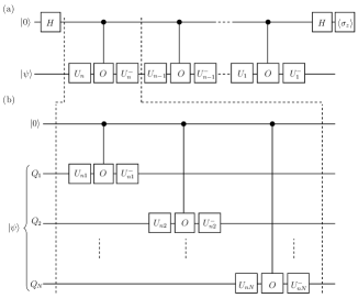
Figure 1: (a) Generalized quantum scattering circuit to measure the $n$ point time correlation function $\langle[O_{1}(t_{1})\otimes O_{2}(t_{1})\dots\otimes O_{N}(t_{1})][O_{1}(t_{2})\otimes O_{2}(t_{2})\dots\otimes O_{N}(t_{2})]\dots[O_{1}(t_{n})\otimes O_{2}(t_{n})\dots\otimes O_{N}(t_{n})]\rangle$, where each observable is a tensor product of $N$ operators, $U^{\mp}_{1}=e^{\pm\frac{iHt_{1}}{\hslash}}$,… $U^{\mp}_{n-1}=e^{\pm\frac{iHt_{n-1}}{\hslash}}$, $U^{\mp}_{n}=e^{\pm\frac{iHt_{n}}{\hslash}}$.The ‘probe’ (ancilla) qubit is initially in the state $|0\rangle$ and the system qubit is in the state $|\psi\rangle$. The correlation function is obtained by measuring the the expectation value $\left\langle\sigma_{z}\right\rangle$ of the ancilla qubit. (b) Expanded schematic of the circuit between dotted lines in panel (a), showing the decomposition of the correlation function $\langle[O_{1}(t_{n})\otimes O_{2}(t_{n})\dots\otimes O_{N}(t_{n})]\rangle$, where $O_{i}(t_{n})$ is measured on the $i$th qubit ($i=1...N$) and $|\psi\rangle$ refers to the initial state of all the system qubits and $U^{\mp}_{n1}=e^{\pm\frac{iHt_{n1}}{\hslash}}$, $U^{\mp}_{n2}=e^{\pm\frac{iHt_{n2}}{\hslash}}$…, $U^{\mp}_{nN}=e^{\pm\frac{iHt_{nN}}{\hslash}}$.

Fig. 1 depicts a schematic diagram of the generalized quantum scattering circuit to generate temporal correlations and demonstrate violation of temporal noncontextuality. The system is prepared in a known initial state, which interacts with the ancilla in such a way that a measurement over its state after the interaction, brings out the information about the system state. The ‘probe qubit’ (ancillary qubit) is prepared in a known initial state and the ‘system qubit’ is prepared in the state for which the observables are to be measured. Consider the input state:

$$\rho_{in}=\rho_{probe}\otimes\rho_{sys}=|0\rangle\langle 0|\otimes|\psi\rangle\langle\psi|$$ (1)

where the ‘probe qubit’ is prepared in the $|0\rangle$ state and the ‘system qubit’ is prepared in the state $|\psi\rangle$. After applying the unitary transformation shown in Fig. 1, the output is given by:

$$\rho_{{\rm out}}=|\psi_{{\rm out}}\rangle\langle\psi_{{\rm out}}|,\,\,{\rm with}$$

$$|\psi_{{\rm out}}\rangle=|0\rangle\otimes(I+U)|\psi\rangle+|1\rangle\otimes(I-U)|\psi\rangle,\,\,{\rm and}$$

$$U=e^{\frac{iHt_{1}}{\hslash}}Oe^{-\frac{iHt_{1}}{\hslash}}e^{\frac{iHt_{2}}{\hslash}}Oe^{-\frac{iHt_{2}}{\hslash}}\cdots e^{\frac{iHt_{n}}{\hslash}}Oe^{-\frac{iHt_{n}}{\hslash}}$$ (2)

The real part of the expectation value of the $z$-component of the spin angular momentum of the ‘probe’ qubit turns out to be related to the expectation values of desired observables of the original state as follows:

$$\langle\sigma_{z}\rangle=Tr[\rho_{sys}U]\quad{\rm therefore},$$

$$\langle\sigma_{z}\rangle=\langle O(t_{1})O(t_{2})...O(t_{n})\rangle$$ (3)

The generalized quantum scattering circuit can be used to experimentally demonstrate those inequalities which involve temporal correlation functions, such as the temporal PM noncontextual inequality and the temporal KCBS inequality. While the ideal negative measurement (INM) protocol described in Ref. Majidy et al. (2019) is similar to our measurement scheme, in the INM protocol the ancilla is coupled to only one of the two measurement outcomes and the protocol hence requires two experimental runs: with a CNOT gate as well as with an anti-CNOT gate. Our circuit on the other hand, requires only a single experimental run and does not require additional CNOT and anti-CNOT gates for its implementation.

III Violation of Temporal PM and Temporal Bell-Type Inequalities

Consider performing a set of five dichotomic (i.e. the measurement outcomes are $\pm 1$) measurements of variables $X_{j},j=1,..5$ on a single system. Each measurement $X_{j}$ is compatible with the preceding and succeeding measurements and the sums are modulo 5. Compatible measurements implies that the joint or sequential measurements of the variables $X_{j}$ do not affect each other, which basically ensures that the measurements are noninvasive. The existence of a joint probability distribution for all the measurement outcomes can be tested by constructing the KCBS inequality Markiewicz et al. (2014):

$$\sum_{j=0}^{4}\langle X_{j}X_{j+1}\rangle\geq-3$$ (4)

where $-3$ is the minimum value for an NCHV model. Noncontextual in this sense implies that the NCHV theory assigns a value to an observable which is independent of other compatible observables being measured along with it. By definition each correlation function is given by Markiewicz et al. (2014):

$$\langle X_{i}X_{j}\rangle=\sum_{x_{i},x_{j}=\pm 1}x_{i}x_{j}p(x_{i},x_{j})$$ (5)

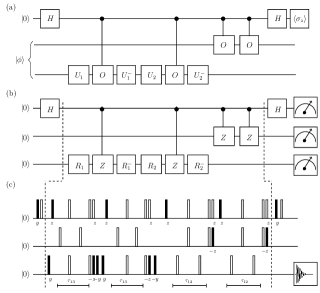
Figure 2: (a) Quantum scattering circuit for measuring the correlation function $\langle A\alpha a\rangle$ involved in the PM inequality, where $O=\sigma_{z}$ and $U^{\pm}_{1,2}=e^{\mp i\sigma_{y}\theta/2}$ with $\theta=\pi/2$. (b) Decomposition of the quantum scattering circuit in terms of rotation operators where $R^{\pm}_{1,2}$ correspond to $(\frac{\pi}{2})_{\pm y}$, $H$ are Hadamard gates and $Z$ are rotations about the $z$ axis. (c) NMR pulse sequence corresponding to the quantum scattering circuit, where filled and unfilled rectangles correspond to $\pi/2$ and $\pi$ pulses, respectively. The time intervals $\tau_{12},\tau_{13}$ are set to $\frac{1}{2J_{HF}}$ and $\frac{1}{2J_{HC}}$, respectively.

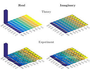
Figure 3: Real (left) and imaginary (right) parts of the theoretical and experimental tomographs of the input $\rho=|0\rangle\langle 0|\otimes|00\rangle\langle 00|$ state in the eight-dimensional Hilbert space, prepared with an experimental state fidelity of 0.964$\pm$0.004.

A “pentagon LG” inequality was constructed wherein Avis et al. (2010)

$$\sum_{1\leq i<j\leq 5}\langle X_{i}X_{j}\rangle+2\geq 0$$ (6)

This inequality has 10 two-time correlation functions which can be computed from one single experiment using compatible measurements. The two-time correlation function turns out to be Markiewicz et al. (2014)

$$\langle X_{i}X_{j}\rangle=\frac{1}{2}Tr[\rho\{X_{i},X_{j}\}]$$ (7)

for a density matrix $\rho$. The five measurable observables were chosen to be Guhne et al. (2014):

$$X_{1}\equiv\sigma_{z}\,,X_{2}\equiv\sigma_{\theta}\,,X_{3}\equiv\sigma_{z}\,,X_{4}\equiv\sigma_{\theta}\,,X_{5}\equiv\sigma_{z}$$ (8)

where $\sigma_{x},\sigma_{z}$ are the Pauli operators and $\sigma_{\theta}\equiv\cos{\theta}\,\sigma_{z}+\sin{\theta}\,\sigma_{x}$. For this set of chosen observables and with $\theta$ chosen such that $\cos{\theta}=-3/4$, the correlation function takes the value Avis et al. (2010)

$$\sum_{1\leq i<j\leq 5}\langle X_{i}X_{j}\rangle=-9/4$$ (9)

which is the smallest possible value and violates the “pentagon” LG inequality given in Eqn. (6).

III.1 The NMR system

We used the molecule of ¹³C -labeled diethyl fluoromalonate dissolved in acetone-D6 as a three-qubit system, with the ¹H, ¹⁹F and ¹³C spin-1/2 nuclei being encoded as ‘qubit one’, ‘qubit two’ and ‘qubit three’, respectively. The NMR Hamiltonian for a three-qubit system in the rotating frame is Oliveira et al. (2007):

$$\mathcal{H}=-\sum_{i=1}^{3}v_{i}I^{i}_{z}+\sum_{i>j,i=1}^{3}J_{ij}I^{i}_{z}I^{j}_{z}$$ (10)

where the indices $i,j$ = 1, 2, or 3 label the qubit, $\nu_{i}$ is the chemical shift of the $i$th qubit in the rotating frame, $J_{{ij}}$ is the scalar coupling interaction strength, and $I_{z}^{{i}}$ is $z$-component of the spin angular momentum operator of the $i^{th}$ qubit. The system was initialized in a pseudopure state (PPS), i.e., $|000\rangle$, using the spatial averaging technique Cory et al. (1998). The fidelity of the experimentally prepared PPS state was computed to be 0.964$\pm$0.004 using the Uhlmann-Jozsa fidelity measure Jozsa (1994); Uhlmann (1976). Quantum state tomography was performed to experimentally reconstruct the density operator using a reduced tomography protocol Leskowitz and Mueller (2004). The $T_{1}$ and $T_{2}$ relaxation times for all three qubits range between 3.7 s - 6.8 s and 1.0 s - 2.8 s, respectively. Nonlocal unitary operations were achieved by free evolution under the system Hamiltonian, of suitable duration under the desired scalar coupling with the help of embedded $\pi$ refocusing pulses. The durations of the $\frac{\pi}{2}$ pulses for ¹H, ¹⁹F, and ¹³C nuclei were 9.55 $\mu$s at 18.14 W power level, 23.00 $\mu$s at a power level of 42.27 W, and 15.75 $\mu$s at a power level of 179.47 W, respectively.

III.2 Experimental violation of the temporal Peres-Mermin inequality

A temporal equivalent of the KCBS inequality can be constructed similarly to the “pentagon LG” inequality by considering a set of nine dichotomic variables, and three successive measurements at two sequential times from the set of time points $t=\{t_{1},t_{2},..t_{5}\}$. The observable set chosen is the “PM square” of nine dichotomous and mutually compatible observables $A,B,C,a,b,c,\alpha,\beta,\gamma$ Guhne et al. (2014):

$$\begin{array}[]{lll}A=\sigma_{z}\otimes I,&B=I\otimes\sigma_{z},&C=\sigma_{z}\otimes\sigma_{z}\\ a=I\otimes\sigma_{x},&b=\sigma_{x}\otimes I,&c=\sigma_{x}\otimes\sigma_{x}\\ \alpha=\sigma_{z}\otimes\sigma_{x},&\beta=\sigma_{x}\otimes\sigma_{z},&\gamma=\sigma_{y}\otimes\sigma_{y}.\end{array}$$ (11)

Consider the combination of expectation values defined as follows:

$$\langle X_{{\rm PM}}\rangle=\langle ABC\rangle+\langle bca\rangle+\langle\gamma\alpha\beta\rangle+\langle A\alpha a\rangle+\langle bB\beta\rangle-\langle\gamma cC\rangle$$ (12)

If we make non-contextual assignments of values we get the inequality

$$\langle X_{{\rm PM}}\rangle\leq 4$$ (13)

which is satisfied by all NCHV theories. This is the temporal PM inequality ($X_{PM}$) Guhne et al. (2014). It has been shown that for a four-dimensional quantum system and a particular set of observables, a value of $\langle X_{PM}\rangle=6$ is obtained for any quantum state, demonstrating state-independent contextuality Cabello (2008).

We note here in passing that in this “PM square” set of measurements, each observable always occurs either in the first place or the second place or the third place in the sequential mean value. This inequality is violated whenever a joint probability distribution cannot be found which assigns predetermined outcomes to the measurements $X_{i}$ at all times $t_{1}...t_{5}$, and this violation is termed contextual in time. The system evolves under the action of a time-independent Hamiltonian $H=\hbar\omega\sigma_{x,y}$, which can be implemented in NMR using suitable rf pulses applied on the qubits. After state preparation, the probe qubit interacts with the system qubit via suitable unitaries. The temporal correlation functions are obtained by measuring the real part of the expectation value of $z$-component of the spin angular momentum of the probe qubit.

Our experimental task is to measure the expectation values of joint probabilities which are measured sequentially. To violate the temporal PM inequality we need to measure the three observables sequentially for any two-qubit state. We experimentally violated the PM inequality by measuring the six correlation functions using the generalized quantum scattering circuit. Fig. 2 shows the quantum scattering circuit, the operator decomposition and the corresponding NMR pulse sequence, to calculate the correlation function $\left\langle A\alpha a\right\rangle$ which is one of the six correlation function used in the PM temporal inequality. The PM temporal inequality is violated for any two-qubit state. The probe qubit is prepared in known $|0\rangle$ state and system qubit is prepared in $|\phi\rangle=|00\rangle$ state. We apply the transformation given in Fig. 2(a), with suitable values of $O=\sigma_{z}$ and $\theta=\pi/2$. The correlation function $\left\langle A\alpha a\right\rangle$ for the $|\phi\rangle=|00\rangle$ state can be obtained by measuring the real part of the expected value of the $z$-component of the spin for the probe qubit. The other correlation functions involved in the PM temporal inequality are measured in a similar fashion.

Since the temporal PM inequality is violated for any two-qubit state, we chose to prepare the probe qubit in a known $|0\rangle$ state and the system qubits were prepared in the $|\phi\rangle=|00\rangle$ state. The experimental tomograph of the state prepared in $\rho=|0\rangle\langle 0|\otimes|00\rangle\langle 00|$ is given in Fig 3, achieved with a fidelity of 0.964$\pm$0.004. We applied the unitary transformations given in Fig. 2 with values of $O=\sigma_{z}$ and $\theta=\pi/2$. The correlation function $\left\langle A\alpha a\right\rangle$ for the $|\phi\rangle=|00\rangle$ state can be obtained by measuring the real part of the expected value of the spin $z$-component of the probe qubit. The other correlation functions involved in the temporal PM inequality are calculated in a similar fashion. The mean value of the correlation functions and their error bars were calculated by repeating the experiment three times and the theoretically expected and experimentally calculated values are given in Table 1. The theoretically computed and experimentally measured values of the correlation functions agree well to within experimental errors. We experimentally violated the temporal PM inequality, obtaining $\langle X_{PM}\rangle_{\rm Expt}=4.667\pm 0.013$, showing the contextual nature of the measured expectation values.

III.3 Experimental violation of a temporal Bell-type inequality

Table 1: Theoretically computed and experimentally measured values of correlations functions corresponding to the PM inequality .

Observables	Theoretical	Experimental
$\langle ABC\rangle$	1	0.928 $\pm$ 0.017
$\langle bca\rangle$	1	0.706 $\pm$ 0.012
$\langle\gamma\alpha\beta\rangle$	1	0.817 $\pm$ 0.010
$\langle A\alpha a\rangle$	1	0.685 $\pm$ 0.008
$\langle bB\beta\rangle$	1	0.755 $\pm$ 0.011
$\langle\gamma cC\rangle$	-1	-0.784 $\pm$ 0.019

The temporal KCBS noncontextual inequality can be constructed by considering a dichotomic variable $X_{t}$ with successive measurements performed at two sequential times drawn from the time instants $t=\{t_{0},t_{1},....,t_{4}\}$. The two-point temporal correlations thus obtained lead to the corresponding temporal KCBS inequality Markiewicz et al. (2014):

$$\sum_{i=0}^{4}\langle X_{t_{i}}X_{t_{i+1}}\rangle\geq-3$$ (14)

The violation of this inequality can be termed as contextuality in time.

The temporal KCBS inequality can be transformed into a Bell-type inequality which tests the existence of a joint probability distribution for measurements on dichotomic variables, performed on subsystems $A$ and $B$. The transformed Bell-type inequality is given as Markiewicz et al. (2014)

$$\left\langle A_{0}B_{1}\right\rangle+\left\langle A_{1}B_{2}\right\rangle+\left\langle A_{2}B_{3}\right\rangle+\left\langle A_{3}B_{4}\right\rangle+\left\langle A_{4}B_{0}\right\rangle\geq-3$$ (15)

where $A_{i}$ and $B_{j}$ are measured on the subsystems with the additional constraint that

$$\langle A_{i}B_{i}\rangle=1\,\,\,{\rm for\,\,\,all}\,\,\,i$$ (16)

which implies that the outcomes of pairs of measurements are the same. Violation of this inequality shows the non-existence of joint probability distribution for this scenario.

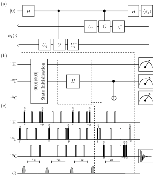
Figure 4: (a) Quantum circuit to measure the correlation function $\langle A_{r}B_{q}\rangle$ involved in the Bell-type inequality, where $U_{r,q}=e^{\frac{-i2\pi r,q}{5}}$, $O=\sigma_{z}$ and $r,q=0,1,2,3,4$. (b) Quantum circuit for state preparation. (c) Corresponding NMR pulse sequence for the quantum circuit. The sequence of pulses before the first dashed black line achieves initialization of the state into the pseudopure $|000\rangle$ state. The unfilled rectangles denote $\pi$ pulses, and the flip angle and phases of the other pulses written below each pulse. The time intervals $\tau_{12}$, $\tau_{13}$, $\tau_{23}$ are set to $\frac{1}{2J_{HF}}$, $\frac{1}{2J_{HC}}$, $\frac{1}{2J_{FC}}$, respectively.

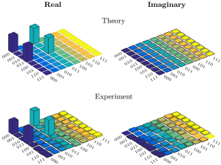
Figure 5: Real (left) and imaginary (right) parts of the theoretically expected and the experimentally reconstructed tomographs of the $\langle\psi_{1}|=\frac{1}{\sqrt{2}}(1,0,0,1,0,0,0,0)$ state in the eight-dimensional quantum system, with an experimental state fidelity of 0.947$\pm$0.009.

We experimentally demonstrated the violation of the transformed Bell-type inequality given in Eqn. 15 using the quantum scattering circuit on the same three-qubit system. Fig. 4(a) shows the quantum scattering circuit to calculate the correlation function $\langle A_{r}B_{q}\rangle$, involved in the transformed Bell-type inequality on an eight-dimensional quantum system. For the violation of the transformed Bell-type inequality, we used the ¹H as the probe qubit and ¹³C and ¹⁹F as the system qubits. We apply the transformations given in Fig. 4(a) with suitable values of $O=\sigma_{z}$ and $q,r=0,1,2,3,4$.

The optimal violation of transformed Bell-type inequality can be obtained for the state $\langle\psi_{1}|=\frac{1}{\sqrt{2}}(1,0,0,1)$ with the probe qubit prepared in the state $|0\rangle$, and for the measurements $A_{j}=\sigma_{j}\otimes I$, $B_{j}=I\otimes\sigma_{j}$ where $j=0,1,2,3,4$ and $\sigma_{j}=e^{i\frac{2\pi j}{5}\sigma_{y}}\sigma_{z}e^{-i\frac{2\pi j}{5}\sigma_{y}}$. The correlation functions $\langle A_{r}B_{q}\rangle$ for the state $\langle\psi_{1}|=\frac{1}{\sqrt{2}}(1,0,0,1)$ can be obtained by measuring the real part of the expected value of the spin $z$-component for the probe qubit. The corresponding quantum circuit for state preparation is shown in Fig. 4(b) and the NMR pulse sequence is shown in Fig. 4 (c). The sequence of pulses before the first dashed black line achieves state initialization into the $|000\rangle$ state. After this we apply the Hadamard gate (on ¹³C), followed by a CNOT₂₃ gate, and the resultant state corresponds to $\rho_{1}=|0\rangle\langle 0|\otimes|\psi_{1}\rangle\langle\psi_{1}|$ with $\langle\psi_{1}|=\frac{1}{\sqrt{2}}(1,0,0,1)$.

The tomograph of the state prepared in $\rho_{1}=|0\rangle\langle 0|\otimes|\psi_{1}\rangle\langle\psi_{1}|$ with $\langle\psi_{1}|=\frac{1}{\sqrt{2}}(1,0,0,1)$ is given in Fig 5 with an experimental fidelity of 0.947$\pm$0.009. The mean values of the correlation functions and their error bars were calculated by repeating the experiment three times and and calculated values are given in Table  2. As seen from the values tabulated in Table 2, the theoretically computed and experimentally measured values of the correlation functions agree well to within experimental errors. We have experimentally violated the transformed Bell-type inequality with the violation of $-3.755\pm 0.008$. When a temporal and a spatial scenario are interconvertible, the corresponding temporal and spatial Tsirelson bounds are always equal and are greater than or equal to the contextual Tsirelson bound Tsirel’son (1987). We also experimentally verified that the Tsirelson bound of the transformed Bell-type inequality is the same as that of the temporal KCBS inequality. For KCBS-type scenarios, the quantum contextual bound is strictly lower than the quantum temporal and nonlocal bound.

Table 2: Theoretically computed and experimentally measured values of quantum correlations corresponding to the Bell-test.

Observables	Theoretical	Experimental
$\langle A_{0}B_{1}\rangle$	-0.809	-0.684 $\pm$ 0.014
$\langle A_{1}B_{2}\rangle$	-0.809	-0.754 $\pm$ 0.006
$\langle A_{2}B_{3}\rangle$	-0.809	-0.756 $\pm$ 0.011
$\langle A_{3}B_{4}\rangle$	-0.809	-0.746 $\pm$ 0.005
$\langle A_{4}B_{0}\rangle$	-0.809	-0.815 $\pm$ 0.004

IV Concluding Remarks

We designed and experimentally implemented a generalized quantum scattering circuit to measure an $n$-point correlation function on an NMR quantum information processor, with an observable being measured sequentially at these $n$ time instants. We experimentally demonstrated the violation of a temporal noncontextuality PM inequality using three NMR qubits, which involved performing sequential noninvasive measurements. We also demonstrated the violation of a transformed Bell-type inequality (analogous to the temporal KCBS inequality) on the same system and showed that the Tsirelson bound of the transformed Bell-type inequality is the same as that of the analogous temporal KCBS inequality. The generalized quantum scattering circuit we have constructed is independent of the quantum hardware used for its implementation and can be applied to systems other than NMR qubits. Our work asserts that NMR quantum processors can serve as optimal test beds for testing such inequalities.