Cauchy-Schwarz Regularized Autoencoder

Abstract

Recent work in unsupervised learning has focused on efficient inference and learning in latent variables models. Training these models by maximizing the evidence (marginal likelihood) is typically intractable. Thus, a common approximation is to maximize the Evidence Lower BOund (ELBO) instead. Variational autoencoders (VAE) are a powerful and widely-used class of generative models that optimize the ELBO efficiently for large datasets. However, the VAE’s default Gaussian choice for the prior imposes a strong constraint on its ability to represent the true posterior, thereby degrading overall performance. A Gaussian mixture model (GMM) would be a richer prior, but cannot be handled efficiently within the VAE framework because of the intractibility of the Kullback-Leibler divergence for GMMs. We deviate from the common VAE framework in favor of one with an analytical solution for Gaussian mixture prior. To perform efficient inference for GMM priors, we introduce a new constrained objective based on the Cauchy-Schwarz divergence, which can be computed analytically for GMMs. This new objective allows us to incorporate richer, multi-modal priors into the autoencoding framework. We provide empirical studies on a range of datasets and show that our objective improves upon variational auto-encoding models in density estimation, unsupervised clustering, semi-supervised learning, and face analysis.

1 Introduction

In recent years, generative models have made have made remarkable progress in learning complex, high-dimensional distributions. Particularly deep generative models can model highly complex datasets, including natural images and speech [1, 2, 3, 4, 5, 6]. Variational autoencoders (VAEs), a class of deep generative models, are likelihood-based models which allow to model high-dimensional distributions in a probabilistic fashion. VAEs approximate the true data distribution by maximizing a tractable lower bound on the marginal likelihood (evidence), also known as the evidence lower bound (ELBO). This is equivalent to minimizing the expected negative log-likelihood and Kullback-Leibler (KL) divergence between approximate posterior and prior. With the introduction of VAEs [1, 2], it has become a popular choice of framework for generative modeling. It is based on well-established theory, its training is simpler and more stable than Generative Adversarial Networks (GANs) [3] and its sampling is more efficient than autoregressive models.

Although there has been a surge of work focused to applying VAEs to image generation tasks and improving its encoder–decoder architectures, the VAE framework is still far from learning generative mechanism for real-world scenarios. One of the main challenges is that VAE samples tend to be blurry. Blurry samples can be attributed to the overly simplistic distribution for the prior [7, 8, 9] or posterior [10] and the overregularization through the KL term of VAE objective [11]. As a result several mechanisms focusing on increasing the expressiveness of the variational posterior density [10, 12, 13, 8, 14, 15, 16, 17] have been proposed. Recent work [18, 19] have shown that the prior plays an essential part balancing the performance of the probabilistic encoder and decoder. In the common case of VAE, the choice of a simple prior, e.g., a Gaussian prior with zero mean and unit diagonal covariance, leads to poor generalization due to overregularization of the approximate posterior. In particular, several approaches use Gaussian mixture models (GMMs) as priors for VAEs [20, 21, 16] to increase model capability. However, these approaches do not allow for closed-form optimization. Estimates with low number of Monte Carlo samples can lead to high variance and thus unstable training. Estimates with higher number of Monte Carlo samples are expensive to compute.

In our work, we addresses the aforementioned challenges by changing the VAE framework into a generative model which is better suited for GMMs. We propose an approach which focuses on the loss-function formulation of the VAE: We substitute the VAE objective function with an explicit regularization scheme based on the Cauchy-Schwarz (CS) divergence. This loss-formulation is no longer a lower bound. Nevertheless, this new approach allows us to use GMMs as effective priors since the Cauchy-Schwarz divergence between GMMs can be computed analytically.

Our main contribution is the Cauchy-Schwarz regularized autoencoder (CSRAE) framework for generative modeling and the introduction of a new objective that provides a closed-form solution on the divergence between GMM prior and variational posterior. Compared to existing variational models, we improve on a range of computer vision based tasks: 1) density estimation, 2) unsupervised clustering, 3) semi-supervised learning and 4) face analysis.

2 Background

In a typical unsupervised learning setting, we are often interested in learning compact representations from unlabelled data. For that, we assume to have a dataset $D$ and define $p_{D}(x)$ be the empirical data distribution defined over i.i.d. samples of $D$. Latent variable models defines a joint (parameterized) probability distribution $p_{\theta}(x,z)$ with $x$ being the observed variables and $z$ being (a set of) latent variables. In the Bayesian setting, the joint probability distribution $p(x,z)$ is assumed to have a prior $p(z)$ and a likelihood $p_{\theta}(x|z)$ and the target distribution is the posterior $p(z|x)$. For simplicity, the prior $p(z)$ is usually a Gaussian or uniform prior which enables efficient optimization.

2.1 Variational Autoencoders

In the typical VAE setting [1], the posterior distribution $p(z|x)$ is intractable because the log-marginal likelihood $p(x)=\int p_{\theta}(x,z)dz$ cannot be computed analytically. Therefore, it is common to introduce a parametric approximation $q_{\phi}(z|x)$ to the intractable posterior and minimize the KL divergence between $q$ and the true posterior $p(z|x)$. This is equivalent to maximizing a lower bound $\mathcal{L}_{\textrm{ELBO}}$ on the log-marginal likelihood, which is given by

$$\begin{split}\log p(x)\geq&\;\mathbb{E}_{q_{\phi}}[\log p_{\theta}(x|z)]-\textrm{D}_{\textrm{KL}}(q_{\phi}(z|x)\parallel p(z))\\ =:&\;\mathcal{L}_{\textrm{ELBO}}(x;\theta,\phi),\end{split}$$ (1)

where $\theta$ are the model parameters of $p$ and $\phi$ are the variational parameters of $q$.

There are various ways to optimize the lower bound (1). For continuous latent variables $z$ it can be done efficiently through a reparameterization of the approximate posterior $q_{\phi}(z|x)$ [1, 2]. If both the prior $p(z)$ and the variational approximation $q_{\phi}(z|x)$ are Gaussian, the KL term in (1) can be computed in closed form [1]. In the common case $p(z)$ is set to be a mean-field approximation (factorizing Gaussian). The mean-field approximation has the advantage of being efficient because it assumes all latent variables to be independent and thus, it simplifies the derivations However, this simplified assumption also leads over-regularization.

Although VAEs are widely used for large-scale approximations, it has been observed that VAEs lack in sample quality because the optimized model simplifies the posterior distribution. Maximizing (1) with respect to the variational parameters $\phi$ amounts to minimizing the KL divergence $\textrm{D}_{\textrm{KL}}(q_{\phi}(z|x)\parallel p(z|x))$ between the approximate posterior and the true posterior. The mean-field variational family is problematic, as the log-marginal likelihood $\log p_{D}(x)$ can only be optimized to the extent we are able to approximate the true posterior using this restricted variational family. As a result, considering richer families of approximate posteriors[10, 15, 22] and richer families of priors [16, 23, 7, 8, 24] have been proposed to improve VAE-based models.

From a maximum likelihood perspective, VAE can be seen as an approach to maximize the likelihood of the model. This equates to the first term of (1). The maximization is regularized by a KL term between approximate posterior and prior (second term of (1)). Motivated by this loss-centric view to minimize the divergence between approximate posterior and prior we diverge from the variational inference principle and propose a constrained optimization objective with the Cauchy-Schwarz divergence to compute the divergence between GMMs analytically.

2.2 Cauchy-Schwarz divergence

Based on the Cauchy-Schwarz inequality

$$\left\lVert x\right\rVert^{2}\left\lVert y\right\rVert^{2}\geq(x^{T}y)^{2},$$

the Cauchy-Schwarz divergence [25] is defined as

$$\textrm{D}_{\textrm{CS}}(q(x)\parallel p(x))= \;-\log\frac{\smallint q(x)p(x)dx}{\sqrt{\smallint p(x)^{2}dx\smallint q(x)^{2}dx}}$$ (2)

$$= \;-\log\smallint q(x)p(x)dx+0.5\log\smallint p(x)^{2}dx$$

$$\;+0.5\log\smallint q(x)^{2}dx.$$ (3)

This is a symmetric metric for any two probability density functions $p$ and $q$, such that $0\leq\textrm{D}_{\textrm{CS}}<\infty$, where the minimum is obtained if and only if $q(z)=p(z)$. Principe et al. [25] also show empirical results that indicate that the CS divergence can be considered an approximation to the Kullback-Leibler divergence.

Analytical solution for mixture of Gaussians The Kullback-Leibler divergence can only be computed in closed form for Gaussians, but not for the more versatile class of Gaussian mixtures. However, the Cauchy-Schwarz divergence can be computed in closed form for Gaussian mixtures [26], a property we will exploit in this paper. For example, let $q(x)=\sum_{n=1}^{N}w_{n}\mathcal{N}(x|\mu_{n},\sigma_{n}^{2})$ and $p(x)=\sum_{m=1}^{M}v_{m}\mathcal{N}(x|\nu_{m},\tau_{m}^{2})$ be two mixture-of-Gaussian distributions with different parameters and different numbers of mixture components. Applying that to the three $\log$ terms of (3) separately, the closed-form expression for the Cauchy-Schwarz divergence between $q$ and $p$ translates into

$$\begin{split}\mathrm{D}_{\mathrm{CS}}=&\;-\;\log\Big{(}\sum_{n=1}^{N}\sum_{m=1}^{M}w_{n}v_{m}z_{n,m}\Big{)}\\ &\;+0.5\log\Big{(}\sum_{n,n^{\prime}}^{N}w_{n}w_{n^{\prime}}z_{n,n^{\prime}}\Big{)}\\ &\;+0.5\log\Big{(}\sum_{m,m^{\prime}}^{M}v_{m}v_{m^{\prime}}z_{m,m^{\prime}}\Big{)},\end{split}$$ (4)

where we define $z_{n,m}$, $z_{m,m^{\prime}}$ and $z_{n,n^{\prime}}$ as

$$z_{n,m}= \;\mathcal{N}(\mu_{n}|\nu_{m},\sigma^{2}_{n}+\tau^{2}_{m})$$ (5)

$$z_{m,m^{\prime}}= \;\mathcal{N}(\nu_{m}|\nu_{m^{\prime}},2\tau^{2}_{m^{\prime}})$$ (6)

$$z_{n,n^{\prime}}= \;\mathcal{N}(\mu_{n}|\mu_{n^{\prime}},2\sigma^{2}_{n^{\prime}}).$$ (7)

A detailed derivation of the analytical form is given in the Appendix (1.2).

3 Cauchy-Schwarz Regularized Autoencoder

We consider the objective to maximize the log-marginal likelihood of the model, i.e.,

$$\max_{\theta}\;\mathbb{E}[\log p_{\theta}(x)]=\max_{\theta}\;\mathbb{E}_{p_{D}(x)}[\log\mathbb{E}_{p(z)}[p_{\theta}(x|z)]],$$ (8)

where the expectation w.r.t. $p_{D}(x)$ is approximated using a sample average over the training data $D$. By using the Jensen’s inequality we can obtain a lower bound to the log-marginal likelihood as

$$\log p_{\theta}(x)=\log\mathbb{E}_{p(z)}[p_{\theta}(x|z)]\geq\mathbb{E}_{p(z)}[\log p_{\theta}(x|z)].$$ (9)

This objective does not regularize the encoding distribution. Sampling from the model once training is completed is difficult and thus, maximizing this objective alone can lead to poor generalization. Similarly as in the VAE framework, we define a mapping $q_{\phi}(z|x)$ which transforms the input $x$ to (probabilistic) features $z$. However, we do not treat $q(z|x)$ as an approximate posterior to the true posterior $p(z|x)$. Rather, we match the approximate posterior to the prior to enforce a way of sampling from the generative model $p_{\theta}(x|z)p(z)$. By adding a regularization $R$ we penalize any deviation between $q_{\phi}(z|x)$ from $p(z)$. Ideally, this regularization is a metric function for which $R>0$ when $q\neq p$ and $R=0$ if and only if $q=p$.

$$\begin{split}\max_{\theta,\phi}\mathbb{E}_{p_{D}(x)}\mathbb{E}_{q_{\phi}(z|x)}[\log p_{\theta}(x|z)]\\ \textrm{ subject to }0\leq R(q_{\phi})<\epsilon.\end{split}$$ (10)

In this formulation $\epsilon$ specifies the magnitude of the applied constraint. If $R$ is defined as KL divergence, we have the original ELBO formulation (1). We divert from this principle and use the Cauchy-Schwarz divergence for regularization to match an approximate posterior to a prior. The advantage is that we can use GMMs, a powerful family of distributions, and calculate the divergence analytically. This enables both prior and approximate posterior to be more flexible.

$$\begin{split}\underset{\theta,\phi}{\max}\;\mathbb{E}_{p_{D}(x)}\Big{[}\mathbb{E}_{q_{\phi}(z|x)}[\log p_{\theta}(x|z)]\Big{]}\\ \text{ subject to }\mathrm{D}_{\mathrm{CS}}(q_{\phi}(z|x)\parallel p(z))<\epsilon.\end{split}$$ (11)

Re-writing (11) as a Lagrangian under the KKT conditions [27, 28], we obtain

$$\begin{split}\mathcal{F}(x;\theta,\phi,\lambda)=&\;\mathbb{E}_{q_{\phi}(z|x)}[\log p_{\theta}(x|z)]\\ &\;-\lambda(\mathrm{D}_{\mathrm{CS}}(q_{\phi}(z|x)\parallel p(z))-\epsilon),\end{split}$$ (12)

where the KKT multiplier $\lambda$ is the regularization coefficient that ensures that the posterior distribution is close to the prior $p(z)$. According to the complementary slackness of the KKT condition and since $\alpha,\epsilon\geq 0$, (12) can be re-written as

$$\mathcal{F}(x;\theta,\phi,\lambda)\geq \;\mathbb{E}_{q_{\phi}(z|x)}[\log p_{\theta}(x|z)]-\lambda\mathrm{D}_{\mathrm{CS}}(q_{\phi}(z|x)\parallel p(z))$$

$$=: \;\mathcal{L}_{\textrm{CSRAE}}(x;\theta,\phi,\lambda).$$ (13)

Decomposing the proposed objective $\mathcal{L_{\textrm{CSRAE}}}(x;\theta,\phi,\lambda)$ yields

$$\begin{split}\mathcal{L}_{\textrm{CSRAE}}=&\;\underbrace{\log p(x)}_{\begin{subarray}{c}\text{log-marginal}\\ \text{likelihood}\end{subarray}}-\underbrace{\textrm{D}_{\textrm{KL}}(q(z|x)\parallel p(z|x))}_{\begin{subarray}{c}\text{KL divergence between}\\ \text{posterior and approx. posterior}\end{subarray}}\\ &+\;\underbrace{\textrm{D}_{\textrm{KL}}(q(z|x)\parallel p(z))}_{\begin{subarray}{c}\text{KL divergence between}\\ \text{approx. posterior and prior}\end{subarray}}-\lambda\cdot\underbrace{\textrm{D}_{\textrm{CS}}(q(z|x)\parallel p(z))}_{\begin{subarray}{c}\text{CS divergence between}\\ \text{approx. posterior and prior}\end{subarray}}.\end{split}$$ (14)

Maximizing $\mathcal{L}_{\textrm{CSRAE}}$ is equivalent to maximizing the log-marginal likelihood, mimimizing the KL divergence between approximate posterior and true posterior and minimizing/maximizing the divergence between approximate posterior and prior.

3.1 Relation to $\beta$-VAE and rate-distortion theory

$\mathcal{L}_{\textrm{CSRAE}}$ is exactly the log-marginal likelihood if $q(z|x)=p(z|x)=p(z)$. The hyperparameter $\lambda$ determines the pressure applied to the regularization during training which encourages different degrees of how well the approximate posterior matches the prior. This improves on sampling from the autoencoding model, but may also decrease the expected log likelihood (reconstruction) under the model. This behaviour is similar to the one of $\beta$-VAE [11]. $\beta$-VAE [11] modified the VAE framework [1, 2] and introduces $\beta$ to adjusting the KL term for better controlling the degree of disentanglement. It has a similar objective, which we can be similarly decomposed as in (14):

$$\begin{split}\mathcal{L}_{\beta}=&\;\mathbb{E}_{q_{\phi}(z|x)}[\log p_{\theta}(x|z)]-\beta\mathrm{D}_{\mathrm{KL}}(q_{\phi}(z|x)\parallel p(z))\end{split}$$ (15)

$$\begin{split}=&\;\underbrace{\log p(x)}_{\begin{subarray}{c}\text{log-marginal}\\ \text{likelihood}\end{subarray}}-\underbrace{\textrm{D}_{\textrm{KL}}(q(z|x)\parallel p(z|x))}_{\begin{subarray}{c}\text{KL divergence between}\\ \text{posterior and approx. posterior}\end{subarray}}\\ &+\;(\beta-1)\cdot\underbrace{\textrm{D}_{\textrm{KL}}(q(z|x)\parallel p(z))}_{\begin{subarray}{c}\text{KL divergence between}\\ \text{approx. posterior and prior}\end{subarray}}.\end{split}$$ (16)

Similar to our approach, the $\beta$-VAE puts a contraint on the similarity between the approximate posterior and the prior through a regularized KL divergence. Both the proposed CSRAE objective $\mathcal{L}_{\textrm{CSRAE}}$ and the $\beta$-VAE objective [11] $\mathcal{L_{\beta}}$ are more general optimization criteria that are not always a lower bound on the log-marginal likelihood. For $\beta$-VAE $\mathcal{L_{\beta}}$ is a lower bound with $\beta\geq 1$. For CSRAE we have a lower bound on the log-marginal likelihood if $\lambda\textrm{D}_{\textrm{CS}}(q(z|x)\parallel p(z))\geq\textrm{D}_{\textrm{KL}}(q(z|x)\parallel p(z))$. However, the inequality cannot be solved analytically for $\lambda$. Similar to $\beta$-VAE [11], we believe there is a trade-off between the quality of the reconstruction and mis-match between prior and approximate posterior. The greater $\lambda$ the closer the approximate posterior is to the prior which improves sampling from the prior. However, this can also degrade the reconstruction due to the pressure of $\lambda$. We treat $\lambda$ as a hyperparameter and optimize for a Pareto optimal solution between reconstruction and constraint, i.e., we perform model selection according to the model achieving $\min\Big{(}\mathbb{E}_{q_{\phi}}[\log p_{\theta}(x|z)]+\textrm{D}_{\textrm{CS}}(q_{\phi}(z|x)\parallel p(z))\Big{)}$ on the validation set.

We can also take an information theoretic perspective as was done in [11, 29, 30] for the KL divergence and which also applies to the Cauchy-Schwarz divergence. Any auto-encoding model can be seen as a communication channel trying to transmit data. The approximate posterior $q(z|x)$ can be considered independent noise channels $z_{i}$ as it has diagonal covariance matrix and thus is factorized. From this perspective, the CS divergence $\textrm{D}_{\textrm{CS}}(q(z|x)\parallel p(z))$ can be seen as the upper bound of number of information required to represent data. If the Cauchy-Schwarz divergence is zero, then each channel $z_{i}$ has zero capacity and thus cannot transmit any data in the channel. The only way to increase the capacity of each channel is to vary the posterior means or decrease the posterior variance. Both ways increase the CS divergence and thus also the capacity.

3.2 Mixture Cauchy-Schwarz regularized autoencoder

One of our main motivations for the proposed constrained optimization objective is to use the Cauchy-Schwarz divergence for a mixture of Gaussian prior. Similar to the constrained problem defined in (13) we now define Mixture Cauchy-Schwarz regularized autoencoder (MixtureCSRAE) using mixture of Gaussian prior. We consider the inference model

$$q_{\phi}(z|x)= \;\mathcal{N}(z|\mu_{\phi}(x),\textrm{diag}(\sigma^{2}_{\phi}(x)))$$ (17)

and the generative model

$$p(z)= \;\frac{1}{K}\sum_{k=1}^{K}\mathcal{N}(z|\mu_{k},\textrm{diag}(\sigma^{2}_{k})),$$ (18)

$$p_{\theta}(x|z)= \;\textrm{Bernoulli}(f_{\theta}(z)).$$ (19)

Similar to the VAE framework we assume the approximate posterior is Gaussian distributed as defined in (17). We parameterize both mixture means $\mu_{\phi}(\cdot)$ and variances $\sigma^{2}_{\phi}(\cdot)$ through an encoding neural network with $x$ as input. A prior put on the approximate posterior is defined as a $K$-component mixture of Gaussians, c.f. (18). The decoder is parameterized by a neural network with weights $\theta$ It uses an appropriate likelihood for the respective data used for optimization, e.g., a Bernoulli likelihood for binary data or the Gaussian likelihood for continuous data. Putting everything together we get the constrained optimization objective

$$\begin{split}\mathcal{L}_{\textrm{MixtureCSRAE}}=&\;\mathbb{E}_{q_{\phi}(z|x)}[\log p_{\theta}(x|z)]\\ &\;-\lambda\textrm{D}_{\textrm{CS}}(q(z|x)\parallel p(z))\end{split}$$ (20)

$$\begin{split}=&\;\mathbb{E}_{q_{\phi}(z|x)}[\log p_{\theta}(x|z)]\\ &\;+\lambda\log\Big{(}\sum_{k}^{K}\mathcal{N}\big{(}\mu_{\phi}|\mu_{k,\psi},\textrm{diag}(\sigma^{2}_{\phi}+\sigma^{2}_{k,\psi})\big{)}\Big{)}\\ &\;-\lambda\log\Big{(}\sum^{K}_{k,k^{\prime}}\mathcal{N}(\mu_{k,\psi}|\mu_{k^{\prime},\psi},\textrm{diag}(2\sigma^{2}_{k^{\prime},\psi}))\Big{)}\\ &\;+\lambda D\log(2\sigma_{\phi}\sqrt{\pi})-\lambda\log K\end{split}$$ (21)

The first term of (21) represents the reconstruction error. The remaining terms optimize the approximate posterior and the prior with $\lambda$ controlling its degree. The second term is maximized if the approximate posterior mean $\mu_{\phi}$ is close to one of the prior means $\mu_{k,\psi},\;k=1,\ldots,K$. The third term penalizes mean priors $\mu_{k,\psi}$ if they are close together and hence, avoids clusters degrading to one cluster. The second last term penalizes the loss term if the approximate posterior increases. The last term can be considered constant w.r.t. to number of clusters. The full derivation of the objective can be found in the Appendix (1.3).

Choice of prior The mixture means and variances of $p(z)$ are easier to set for lower-dimensional cases. However, setting mixture parameters in high dimensions is non-trivial. Therefore, similar to VampPriorVAE [31], we learn the parameters of $p(z)$ through a neural network. There are two kinds of priors we will investigate for our evaluation:

1. mixture of Gaussians prior (MoGPrior):

   $$p(z)=\frac{1}{K}\sum_{k=1}^{K}\mathcal{N}(z|\mu_{k},\textrm{diag}(\sigma^{2}_{k}))$$ (22)

2. variational mixture of posteriors prior (VampPrior) which uses the generative decoder to learn representative pseudo-inputs ($u_{k}$ of the data:

   $$p(z)=\frac{1}{K}\sum_{k=1}^{K}q_{\phi}(z|u_{k}).$$ (23)

The first prior requires more parameters for tuning as it is defined in a general way and there are multiple ways for implementation. The VampPrior which was also used in VampPriorVAE [31] is simple to apply as it uses the encoder to output mixture means and variances. However, it is also prone to overfitting.

3.3 Semi-Supervised Learning

In the semi-supervised setting we consider a labelled dataset $D=\{(x_{1},y_{1}),\ldots,(x_{N},y_{N})\}$, composed of observations $x_{i}$ and corresponding class labels $y_{i}\in\{1,\ldots,K\}$ where $K$ equals to the total number of classes. In this setting, only a small part of the dataset is labelled. Therefore, we split the dataset $D$ into two subsets: $D_{l}$ for labelled training and $D_{ul}$ for unlablled training with $D_{l}\cup D_{ul}=D$ and $D_{l}\cap D_{ul}=\emptyset$. The labels are used to condition the probabilistic model. In the unsupervised subsetting, we treat the label as a second latent variable. We refer to Kingma et al. [32] for the generative and inference model.

For this semi-supervised model we have to consider two cases, the supervised and unsupervised objective. In the supervised case, the labels are observed and we can perform inference on $z\sim q_{\phi}(z|x)$ only. Thus, we have the following constrained optimization objective:

$$\begin{split}\max_{\theta,\phi}\mathbb{E}_{p_{D_{l}}}\Big{[}\mathbb{E}_{q_{\phi}(z|x)}(\log p_{\theta}(x|z,y)\Big{]}\\ \textrm{subject to }0<\mathrm{R}(q_{\phi}(z|x)\parallel p(z))<\epsilon_{1}\\ \textrm{subject to }0<\mathrm{R}(q_{\phi}(y|x)\parallel p(y))<\epsilon_{2}.\end{split}$$ (24)

As defined before in (10), $R$ penalizes deviation from approximate posterior and prior. For the latent variable $z$ we chose $R$ to be the Cauchy-Schwarz divergence. This allows for an analytical solution of mixture of Gaussians. For the (latent) variable $y$ we chose $R$ to be a KL divergence. This choice allows for an analytical solution of Categorical variables. Further, it is similar to the choice made by Kingma et al. [32] and thus, allows for a fair comparison in the evaluation as the objective only differs in the choice of divergence and prior for $z$. As a result, we have the following objective for labelled observations:

$$\begin{split}\mathcal{L}_{\textrm{ssl}}(x,y)=&\;\mathbb{E}_{q_{\theta}(z|x)}[\log p_{\theta}(x|z,y)]\\ &\;-\lambda\textrm{D}_{\textrm{CS}}(q(z|x)|p(x))\\ &\;-\beta\textrm{D}_{\textrm{KL}}(q(y|x)|p(y)).\end{split}$$ (25)

In the unsupervised case, the label is treated as a latent variable over which we marginalize for inference.The resulting objective for handling data points with an unobserved label $y$ is

$$\mathcal{U}_{\textrm{ssl}}(x)=\sum_{y}\mathcal{L}_{\textrm{ssl}}(x,y).$$ (26)

The final objective function is

$$\begin{split}\mathcal{J}=&\;\mathbb{E}_{x,y\sim p_{D_{l}}}[\mathcal{L}_{\textrm{ssl}}(x,y)]+\mathbb{E}_{x\sim p_{D_{u}}}[\mathcal{U}_{\textrm{ssl}}(x)]\\ &\;+\alpha\mathbb{E}_{x,y\sim p_{D_{l}}}[q_{\phi}(y|x)].\end{split}$$ (27)

This objective combines both supervised and unsupervised objectives as defined before and adds a classification as done in [32]. This ensures that the overall objective and in particular the distribution $q_{\phi}(y|x)$ also learn from from the labelled data.

Multi-output labels When learning multi-output labels, we have labels $y\in\{0,1\}^{L}$ where $L$ is the number of ouputs. We assume a factorized prior for $y$ given by $p(y)=\prod_{i=1}^{L}p(y^{i}),\;p(y^{i})=\textrm{Cat}(y|\pi)$. If using the semi-supervised model described before, the unlabelled objective requires marginalizing over all possible label classes. In the setting of a label with $L$ outputs $y\in\{0,1\}^{L}$ marginalizing over all possible label combinations equals to $2^{L}$ possible combinations. Instead we approximate $y$ by sampling from the Gumbel-Softmax distribution [33].

4 Evaluation

Our primary goal is to quantitatively and qualitatively assess properties of the newly proposed CSRAE and Mixture CSRAE. Further, we would like to answer the following questions for the evaluation:

1. Do CSRAE and MixtureCSRAE improve on sample quality compared to VAE and its variants?

2. Can the learned latent embedding used for clustering related tasks?

3. Can CSRAE and MixtureCSRAE be applied for semi-supervised learning and face-related tasks?

4.1 Experimental setups

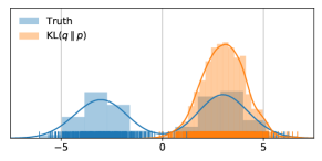
(a) KL divergence with univariate Gaussian

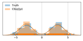
(b) CS divergence with mixture of two Gaussians

Figure 1: The true posterior is a mixture of two univariate Gaussians (blue). The approximate posterior is a univariate Gaussian for KL and a mixture of univariate Gaussians on the right (orange). The KL approximation is on the left (a), the CS approximation on the right (b).

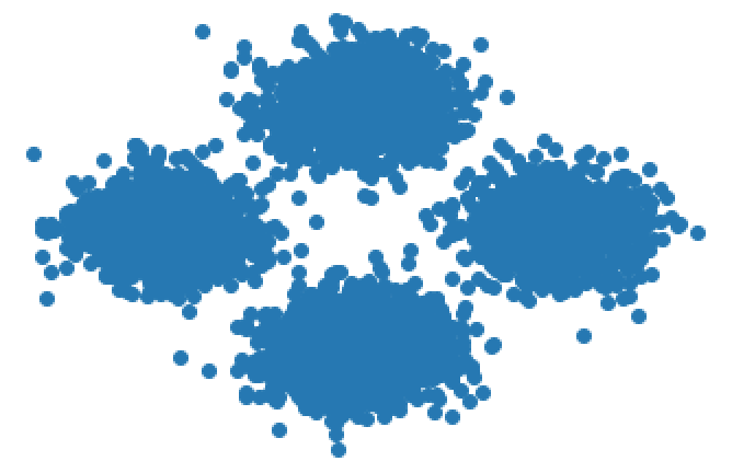
(a) Prior

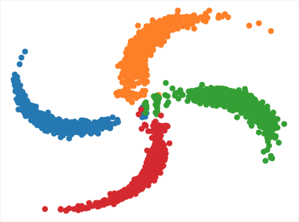
(b) $\lambda=0.5$

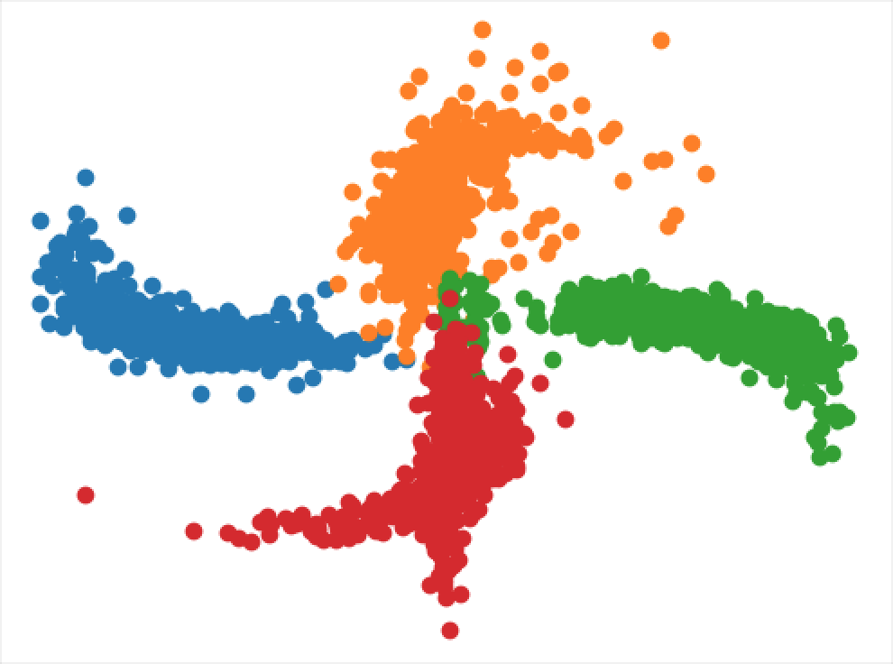
(c) $\lambda=1.0$

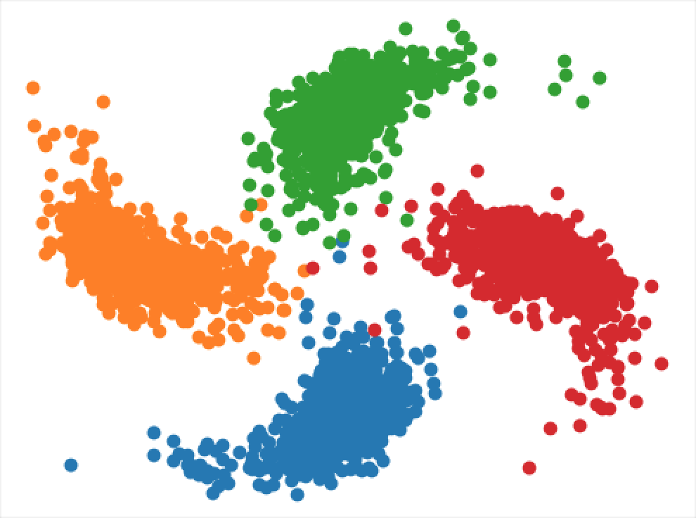
(d) $\lambda=2.5$

(e) $\lambda=5.$

(f) $\lambda=10.$

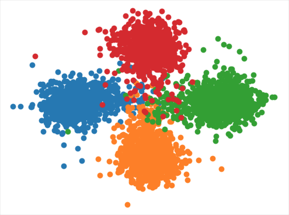
(g) $\lambda=20.$

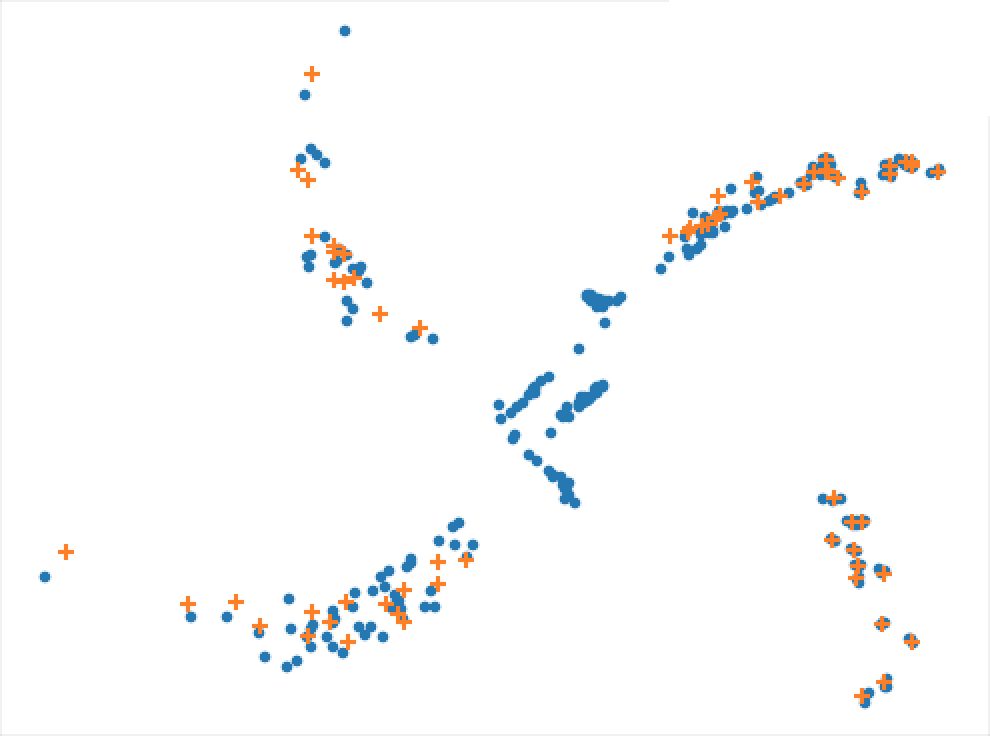
(i) $\lambda=0.5$

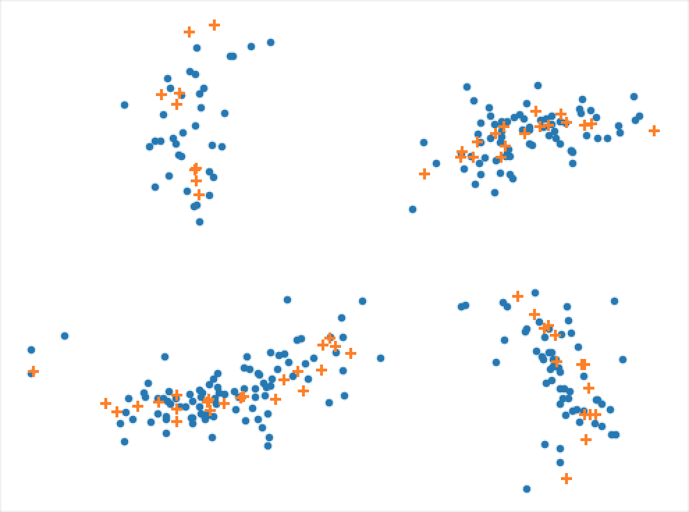
(j) $\lambda=1.0$

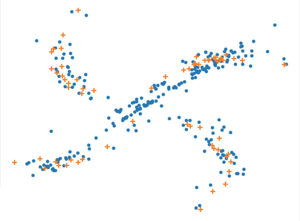
(k) $\lambda=2.5$

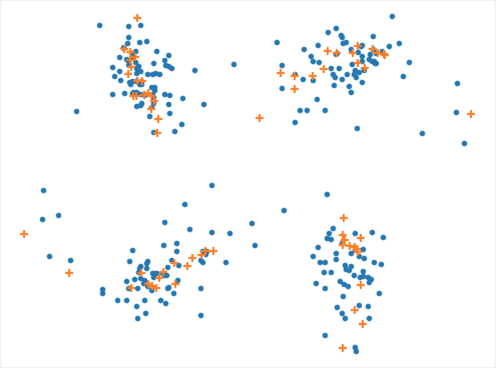
(l) $\lambda=5.$

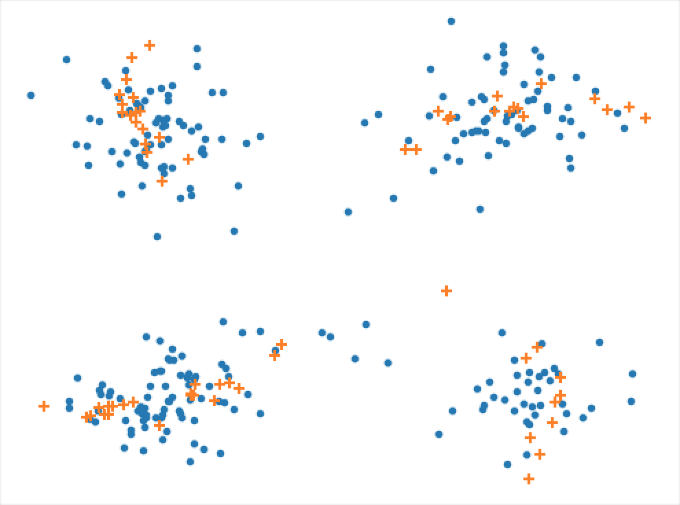
(m) $\lambda=10.$

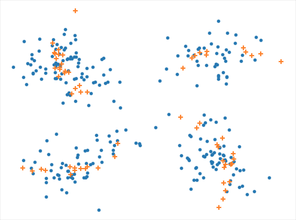
(n) $\lambda=20.$

Figure 2: Visualization of latent embeddings (row 1) and reconstruction (row 2) for different $\lambda$ for pinwheel dataset with mixture of Gaussian prior. The colors in the first rows b)-g) represents the true data class. Best viewed in color.

  
  

(h) Data

Datasets. We consider two toy datasets used for Section 4.2. A 1D mixture of two Gaussians $p(z)=\frac{1}{2}\mathcal{N}(z;-3,1)+\frac{1}{2}\mathcal{N}(z;3,1)$ is used to visualize the challenge of fitting a univariate Gaussian to a Gaussian mixture. We use 2000 i.i.d. samples for training. Further, we use the “pinwheels” dataset from [18]. We generated spiral cluster data with $N=4000$ observations, equally clustered in four spirals with radial and tangential standard deviations respectively of $0.05$ and $0.25$, and a rate of $0.25$. For density estimation, kNN clustering, and semi-supervised learning we carried out experiments using five image datasets: static MNIST [34], dynamic MNIST [35], Omniglot [36], Caltech 101 Silhouette [37] and CIFAR10 [38]. For semi-supervised facial action unit recognition we use DISFA [39] and FERA2015 [40]. For both datasets DISFA and FERA2015 the frames with intensities equal or greater than 2 are considered as positive while others are treated as negative. Further, we performed subject-independent 3-fold cross-validation for these two datasets. Details about all datasets can be found in the Appendix (3.1).

Model architecture. For the toy experiment with the Pinwheel dataset we used a neural network with two fully-connected and Softplus activation. In the experiments for MNIST (static and dynamic), Omniglot, and Caltech 101 Silhouettes we modeled all distributions using fully-connected neural networks with two hidden layers of $300$ hidden units in the unsupervised setting. For CIFAR10 we employed a convolutional architecture with residual blocks similar to [41] whereas for DISFA and FERA2015 we used a convolutional encoder and decoder pair. The detailed listing of all architecture used can be found in the Appendix (3.1). For the toy dataset we used a Gaussian likelihood, for all colored images we used the discretized logistic likelihood as in  [15], and for the other datasets we used a Bernoulli likelihood.

Optimization and hyperparameters All model weights of the neural networks were initialized according to [42]. For fitting a mixture of two Gaussians in Subsection 4.2, we use gradient descent with a learning rate of $0.001$ for both KL and CS minimization. For training all other models, we used the ADAM algorithm [43], where we set the learning rate to $5\cdot 10^{-4}$ and mini-batches of size $100$. Additionally, we used the linear warm-up [44] for 100 epochs to avoid early collapse of the latent variable due to the divergence regularization. During training, we used early-stopping with a look ahead of $100$ iterations to prevent over-fitting. For semi-supervised learning of DISFA and FERA2015 we perform optimization in two phases. First, we only train in an unsupervised fashion without any labels. Subsequently, we used the pre-trained model to include semi-supervised training with labels. Further, due to the imbalance of both datasets’ label distribution, we also used iterative balanced batches during training. For further details, we refer to the Appendix (Section 3.2).

Evaluation metrics We report all evaluation metrics on the test set based on the best validation loss from training. In fact, the log-marginal likelihood (LL) has been the default evaluation metric for models optimizing the LL or ELBO. The marginal likelihood can be computed generating $S$ samples from the recognition model using importance sampling and using the following estimator:

$$p(x)\approx\frac{1}{S}\sum_{s=1}^{S}\frac{p(x|f(\xi^{(s)}))p(\xi^{(s)})}{q(\xi^{(s)|x)})},\;\xi^{(s)}\sim q(\xi|x).$$ (28)

However, Theis et al. [45] showed that high LL does not necessarily correspond to plausible samples and thus is not a suitable metric for assessing image quality. Furthermore, in our own experiments, we observed that while the LL often increased by a large margin, neither the FID nor manual inspection showed improvement in image quality. For these reasons we report the Fréchet inception distance (FID) for density estimation. The FID is a measure of similarity between two datasets of images and is often used to evaluate the fidelity of samples from Generative Adversarial Networks [3]. Heusel et al. [heusel2017gans] showed that this measure correlates with human perception of visual quality and can detect mode collapses in contrast to Inception Score (IS) [SalimansGZCRCC16].

The Fréchet inception distanceuses embeddings from the Inception v3 model to calculate the means and covariances of the real samples $(m,C)$ and the generated samples $(m_{w},C_{w})$. The metric is calculated using the Wasserstein-2 distance between these means and covariances.

$$\begin{split}d^{2}((m,C),(m_{w},C_{w}))&=\left\lVert m-m_{w}\right\rVert^{2}_{2}\\ &\quad+\textrm{Tr}(C+C_{w}-2(CC_{w})^{1/2}).\end{split}$$ (29)

Further, for clustering classification error rate and for facial action unit recognition F1 score was used for evaluation.

4.2 Empirical analysis

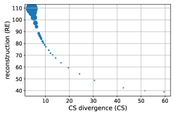
(a) Trade-off between test reconstruction (RE) and test CS divergence with respect to $\lambda$. The scatter marker size indicate the value of $\lambda$ (the greater the marker size the higher $\lambda$).

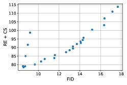
(b) Relationship between model selection criterion $\min(\mathbb{E}_{q}(\log p(x|z))-\textrm{D}_{\textrm{CS}}(q\parallel p))$ (RE + CS, lower is better) and Fréchet inception distance(FID, lower is better)

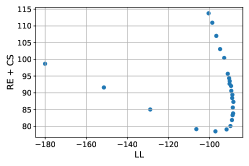
(c) Relationship between model selection criterion $\min(\mathbb{E}_{q}(\log p(x|z))-\textrm{D}_{\textrm{CS}}(q\parallel p))$ (RE + CS, lower is better) and log-marginal likelihood (LL, lower is better)

Figure 3: Ablation for demonstrating effect of constraint $\lambda$ on model selection criterion, log-marginal likelihood (LL) and Fréchet inception distance(FID). All experiments were conducted with dynamic MNIST. We considered $\lambda$ in range of [0.25, 0.5, 0.75, …, 9.5, 9.75, 10.0].

Fitting a mixture of two Gaussians Consider a one-dimensional mixture of Gaussians as the posterior of interest

$$p(z)=\frac{1}{2}\mathcal{N}(z;-3,1)+\frac{1}{2}\mathcal{N}(z;3,1).$$ (30)

The posterior contains multiple modes. We seek to approximate it with two objectives: Kullback-Leibler (KL) with a Gaussian approximating family and Cauchy-Schwarz (CS) with a mixture of Gaussians approximating family. In both settings we can calculate the divergence analytically. Figure 1(a) displays the posterior approximations. We find that the KL divergence chooses a single mode and has slightly different variances. This approximation does not produce good results because a single Gaussian is a poor approximation of the mixture. The approximate posterior in Figure 1 (b) comes from a using a mixture of Gaussian prior. Because this enables the prior to be more general it can capture the posterior.

Visualizing the effect of $\lambda$. We made the assumption that constrained optimization is important for enabling CSRAE models to learn multi-modal representations. One way to view $\lambda$ is as a coefficient balancing the reconstruction and and prior-matching term of the CSRAE object. We visualized this effect in Figure 2(a) where we applied our MixtureCSRAE objective from (21) to the pinwheel toy dataset. The prior visualized in Figure 2(a) (a) is defined as

$$p(z)= \;\sum_{k=1}^{K}\pi^{k}\mathcal{N}(z;\mu_{k},\sigma_{k})$$ (31)

$$= \;\sum_{k=1}^{K}\pi^{k}\prod_{d=1}^{D}\mathcal{N}(z_{d},\mu^{k}_{d},\sigma^{k}_{d}),$$ (32)

with $D=2$, $K=4$, $\sigma^{k}=0.05I_{D}$, $\pi^{k}=\frac{1}{K}$ and $\mu_{d}^{k}\in\{0,1\}$. We observe that with a low $\lambda$ value, e.g., $\lambda=0.5$, the model can reconstructthe input data (Figure 2(a) (i)) almost perfectly, however, the structure of the latent variable depicted in Figure 2(a) (b) is not similar to prior visualized in Figure 2(a) (a). As $\lambda$ is increased, the latent space embedding (Figures 2(a) (b-g)) draws nearer to the prior, the reconstruction decreases in quality resulting the reconstructed datapoints to be less aligned to the original input data.

Model selection and relationship to LL and FID. As shown in Figure 2(a) there is a trade-off between the reconstruction and prior-matching-term–the two terms which make up our loss objective. The trade-off is influenced by $\lambda$. The higher $\lambda$ the more weight is put on the approximate posterior matching the prior and the less weight is put on the reconstruction error. We conducted ablation studies with CSRAE on dynamic MNIST shown in Figure 3 to understand the effect of $\lambda$ on the loss terms and the relationship between loss objective and evaluation metrics FID and LL. Figure 3(a) shows reconstruction loss (y-axis) and prior-matching-term (x-axis) with respect to $\lambda$. In this Figure the marker size is an indicator of the value of $\lambda$, i.e., the greater the marker size the higher the value of $\lambda$. We can observe a gradual decrease in reconstruction error with decreasing $\lambda$ while simultaneously the CS term increases. We added both terms together and plotting them against LL (Figure 3(c)) and FID (Figure 3(b)). The plots visualizes that our model selection criteria $\min\Big{(}\mathbb{E}_{q_{\phi}}[\log p_{\theta}(x|z)]+\textrm{D}_{\textrm{CS}}(q_{\phi}(z|x)\parallel p(z))\Big{)}$ seems proportional to evaluation metrics LL and FID. When our model selection criteria is lowest, FID is at its lowest as well. For LL, we also observe a low $\min\Big{(}\mathbb{E}_{q_{\phi}}[\log p_{\theta}(x|z)]+\textrm{D}_{\textrm{CS}}(q_{\phi}(z|x)\parallel p(z))\Big{)}$ means low LL, however, LL does not necessarily obtain its minimum at the lowest model selection criteria.

Number of mixture components. We compared our MixtureCSRAE with varying number of mixture components. Figure 4 visualizes the LL depending on the number of mixture components ($10,20,40,100,200,300,400,1000$) and the number of latent dimensions ($10,20,40,128$). We observe a trend of increased performance with increasing number of mixture components. But this trend is not retained for larger number of mixtures ($>400$) as performance either drops or remain unchanged. For MoGPrior this drop in performance could be due to increased difficulty to learn a large GMM prior while simultaneously optimizing the approximate posterior parameters. For VampPrior an increase in number of mixture components could aggravate overfitting and thus lead to a performance decrease.

Figure 4: Comparing MoGPrior and VampPrior with varying latent variable dimensions and number of mixtures. We report average ($n=5$) loss (greater is better), c.f. model selection criterion. All solid lines represent MoGPrior with different number of latent dimensions, while all dashed lines represent VampPrior.

MoGPrior vs. VampPrior. When comparing MoGPrior and VampPrior in our ablation study visualized in Figure 4, we can see that the learned prior (MoGPrior) either is of similar or superior performance to VampPrior. The difference in performance is usually smaller for lower number of mixture components ($<100$). However, the gap is more obvious for larger number of mixture components and larger latent dimensions. As mentioned before overfitting of VampPrior might be the reason for this gap.

4.3 Density estimation on common benchmarks

Model	Dataset
	Static	Dynamic	Omniglot	Caltech101	CIFAR10
	MNIST	MNIST
VAE [1] ($z=40$)	10.04 $\pm$ 0.01	10.99 $\pm$ 0.01	9.09 $\pm$ 0.01	18.08 $\pm$ 0.02	11.36 $\pm$ 0.01
VAE [1] ($z=128$)	10.23 $\pm$ 0.02	11.11 $\pm$ 0.01	8.95 $\pm$ 0.02	17.89 $\pm$ 0.04	11.58 $\pm$ 0.01
IWAE [46]	9.87 $\pm$ 0.01	10.97 $\pm$ 0.01	9.13 $\pm$ 0.02	18.03 $\pm$ 0.02	16.15 $\pm$ 0.00
($z=40,n_{\textrm{iw}}=5$)
IWAE [46]	9.83 $\pm$ 0.01	10.92 $\pm$ 0.01	8.40 $\pm$ 0.01	17.47 $\pm$ 0.03	-
($z=128,n_{\textrm{iw}}=50$)
VampPriorVAE [31]	11.64 $\pm$ 0.03	12.69 $\pm$ 0.03	8.88 $\pm$ 0.01	17.45 $\pm$ 0.04	11.19 $\pm$ 0.02
($z=40,k=10$)
VampPriorVAE [31]	10.35 $\pm$ 0.03	11.35 $\pm$ 0.04	8.86 $\pm$ 0.01	17.70 $\pm$ 0.04	11.12 $\pm$ 0.02
($z=40,k=100$)
VampPriorVAE [31]	10.01 $\pm$ 0.04	11.10 $\pm$ 0.02	8.76 $\pm$ 0.01	17.70 $\pm$ 0.05	11.09 $\pm$ 0.03
($z=40,k=400$)
CSRAE ($z=40$)	7.60 $\pm$ 0.01	7.88 $\pm$ 0.02	8.13 $\pm$ 0.02	17.15 $\pm$ 0.05	10.94 $\pm$ 0.03
MixtureCSRAE	7.67 $\pm$ 0.02	7.81 $\pm$ 0.02	8.12 $\pm$ 0.01	17.44 $\pm$ 0.03	10.92 $\pm$ 0.02
($z=40,k=10$)
MixtureCSRAE	7.68 $\pm$ 0.02	7.89 $\pm$ 0.01	7.96 $\pm$ 0.01	16.33 $\pm$ 0.03	10.65 $\pm$ 0.03
($z=40,k=100$)
MixtureCSRAE	7.74 $\pm$ 0.01	8.03 $\pm$ 0.01	7.90 $\pm$ 0.01	16.66 $\pm$ 0.03	10.54 $\pm$ 0.02
($z=40,k=400$)

TABLE I: Average test Fréchet inception distance (FID, $n=5$) and standard error (lower is better). For CIFAR10, IWAE [46] was not computed for dimensions $z=128$ and number of importance weights $k=50$, as this would have been too computationally expensive due to the residual networks used for encoder and decoder.

Quantitative results. We quantitatively evaluate our method using the FID. In Table I we present a comparison between our proposed approach (CSRAE, MixtureCSRAE) and variational auto-encoding models VAE [1], IWAE [46] and VampPriorVAE [31]. The comparison includes training MLP-based models for static and dynamic MNIST, Omniglot and Caltech 101 Silhouettes as well convolutional model with residual blocks for CIFAR10. For fair comparison, we trained all models with the same optimization scheme and model architecture. First, we notice that in all cases the application of the CSRAE and MixtureCSRAE results in a substantial improvement of the generative performance in terms of the test FID, accounting for at least 4% (CIFAR10) and up to 22% (Dynamic MNIST) improvement in performance. Further, for more complex datasets like Omniglot, Caltech101, and CIFAR10, we also observe that a multi-modal prior (MixtureCSRAE) improves upon performance compared to a simple Gaussian prior (CSRAE).

Qualitative results. We plotted both test samples next to its reconstruction in Figure 5(b) for IWAE, VampPriorVAE and MixtureCSRAE. We notice with IWAE and VampPriorVAE that the reconstructions are often smooth even though the original samples had certain missing pixel and/or are distorted. With MixtureCSRAE the reconstructions seems to be more true to its original samples. Furthermore, IWAE seems to fail to reconstruct CIFAR samples. In comparison to VampPriorVAE, we noticed that MixtureCSRAE seems to be visually richer in contrast and sharper. We also visualized samples generated from the best performaning models in Figure 6(c). Similar to the reconstructions the samples of IWAE and VampPriorVAE are smoother and offer less diversity than MixtureCSRAE. Further, MixtureCSRAE samples for CIFAR10 appear to look sharper and richer in contrast. The diversity in samples is also shown in Figure 7 where we visualize samples from individual components of the Mixture of Gaussian prior. The samples are taken from best performing MixtureCSRAE with a Mixture of Gaussian prior of 100 components and trained with Dynamic MNIST and Caltech101. The samples show that each component covers a specific digit of MNIST or a specific shape of Caltech101, and also exemplifies the capability of each component covering diversity within class samples.

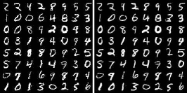
(a) Static MNIST (IWAE)

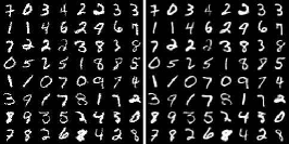
(b) Static MNIST (VampPriorVAE)

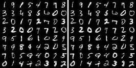
(c) Static MNIST (MixtureCSRAE)

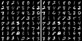
(d) Dynamic MNIST (IWAE)

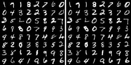
(e) Dynamic MNIST (VampPriorVAE)

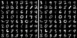
(f) Dynamic MNIST (MixtureCSRAE)

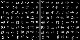
(g) Omniglot (IWAE)

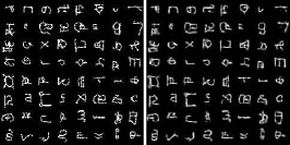
(h) Omniglot (VampPriorVAE)

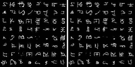
(i) Omniglot (MixtureCSRAE)

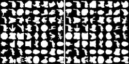
(j) Caltech101 (IWAE)

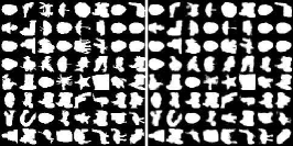
(k) Caltech101 (VampPriorVAE)

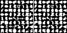
(l) Caltech101 (MixtureCSRAE)

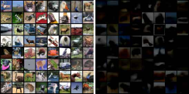
(m) CIFAR10 (IWAE)

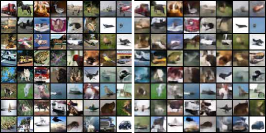
(n) CIFAR10 (VampPriorVAE)

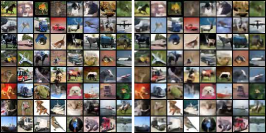
(o) CIFAR10 (MixtureCSRAE)

Figure 5: Test samples and reconstructions of Static MNIST (a)-(c), Dynamic MNIST (d)-(f), Omniglot (g)-(i), Caltech101 (j)-(k) and CIFAR10 (m-o). We showed samples and reconstruction of IWAE (first column), VampPriorVAE (second column) and MixtureCSRAE (third column).

                                

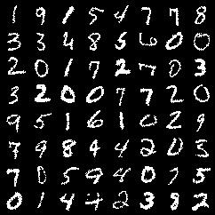
(a) Static MNIST

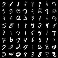
(b) IWAE

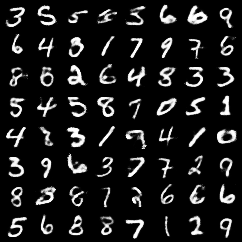
(c) VampPriorVAE

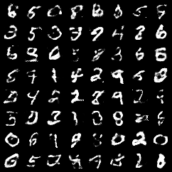
(d) MixtureCSRAE

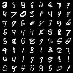
(f) IWAE

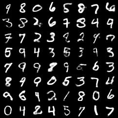
(g) VampPriorVAE

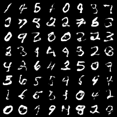
(h) MixtureCSRAE

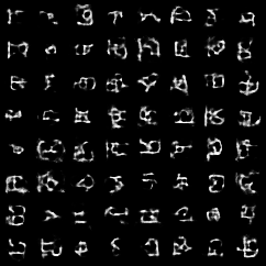
(j) IWAE

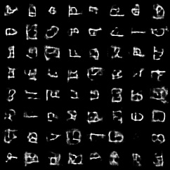
(k) VampPriorVAE)

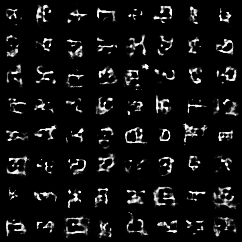
(l) MixtureCSRAE

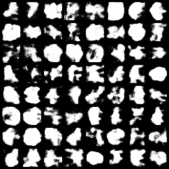
(n) IWAE

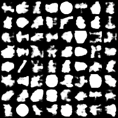
(o) VampPriorVAE

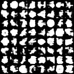
(p) MixtureCSRAE

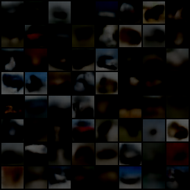
(r) IWAE

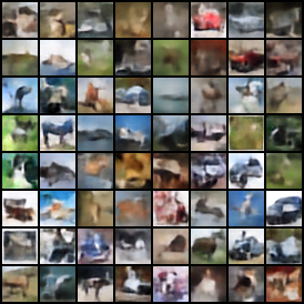
(s) VampPriorVAE

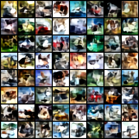
(t) MixtureCSRAE

Figure 6: Test samples (first column) and samples generated from IWAE (second column), VampPriorVAE (third column) and MixtureCSRAE (fourth column)

     
      
      
      
     

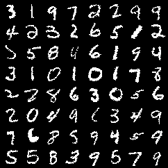
(e) Dynamic MNIST

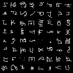
(i) Omniglot

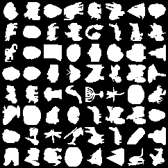
(m) Caltech101

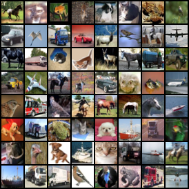
(q) CIFAR10

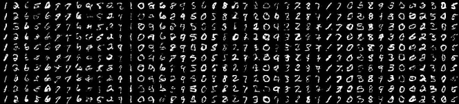
(a) Dynamic MNIST

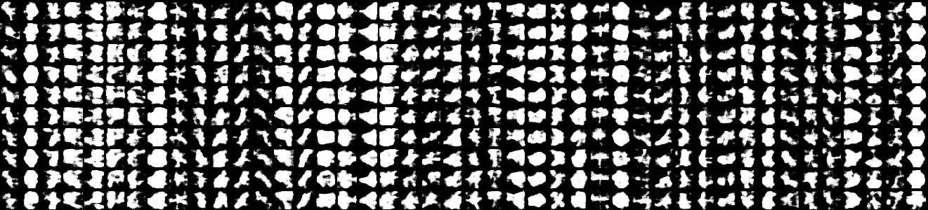
(b) Caltech101

Figure 7: Samples from MixtureCSRAE with a 100-component mixture of Gaussian prior trained with Dynamic MNIST (a) and Caltech101 (b). Each column of the samples represents samples coming from one component of the mixture of Gaussian.

4.4 Clustering

We compared the discriminative qualities of the model by using a k-Nearest Neighbors (kNN) on the latent samples of the test set of dynamic MNIST. Table II show the results of CSRAE compared to the standard VAE (S-VAE) as well as related models, namely, the Gaussian mixture Variational Autoencoder (GMVAE) [20], the deep latent Gaussian mixture model (DLGMM) [8] and the Stick-Breaking Variational Autoencoder (SB-VAE) [9]. For all models we used best top-1 accuracy on the validation for model selection and report the test accuracy for kNN with $k\in\{3,5,7\}$ in Table II. We observed that settings that worked well for density estimation might not work well for kNN. Especially, we experienced an increase in classification error when using larger latent dimensions of $>20$. This decrease in performance can be attributed to the curse of dimensionality. As kNN uses Euclidean distance as default distance metric it becomes meaningless as latent dimension increases. Therefore, for all methods we only report latent dimensions of $[10,20]$. Table II shows that without exception MixtureCSRAE outperforms all models when using latent samples for kNN. Our model improved kNN classification error by at least 2.65% (Caltech101, $k=5$) to at most 25.12% (Dynamic MNIST, $k=3$).

	Dataset
	Dynamic MNIST			Caltech101
Method	$k=3$	$k=5$	$k=10$	$k=3$	$k=5$	$k=10$
VAE ($z=10$)	5.20	4.78	4.52	41.35	40.10	40.26
VAE ($z=20$)	7.04	6.01	5.32	39.62	38.99	39.20
VampPriorVAE [31]	4.92	4.79	4.90	41.74	39.90	40.91
($z=10,k=400$)
VampPriorVAE [31]	3.98	3.87	3.77	38.26	37.64	38.52
($z=20,k=400$)
CSRAE ($z=10$)	4.22	3.93	3.81	41.39	39.73	40.32
CSRAE ($z=20$)	6.03	5.27	4.82	39.75	39.06	39.54
MixtureCSRAE	3.91	3.79	3.78	37.88	37.62	36.75
($z=10,k=400$)
MixtureCSRAE	2.98	2.95	2.94	39.66	37.54	34.94
($z=20,k=400$)

TABLE II: Average classification test error ($n=5$), lower is better. kNN classification was applied with different number of neighbours ($k=[3,5,10]$) on latent samples for dynamic MNIST and Caltech101.

4.5 Semi-supervised learning

As introduced in Section 3.3 we evaluate our semi-supervised approach with MNIST for digit classification as well as DISFA [39] and FERA2015 [47]. The results for MNIST is shown in Table III(a). For all models we used the same architecture and optimization and report results on different number of labels used during training. For every model setting we report the average of five runs with different random seeds. When directly comparing VAE and CSRAE as well as VampPriorVAE and MixtureCSRAE our models improved average classification by at least 0.7% (VAE vs. CSRAE) and at most 12.89% (VampPriorVAE vs MixtureCSRAE).

DISFA [39] and FERA2015 [47] are face datasets which evaluates learning of facial action units. These datasets have labelled facial action units according to the Facial Action Coding System (FACS) [48] which define a set of facial muscle movements. FACS allows to encode any anatomically possible facial expression and have shown wide applications in face and emotion recognition as well as mental health analysis. Most of the existing approaches for AU recognition are supervised and require a large number of facial action unit labels. However, FACS-based labelling is time-consuming and require expert knowledge. Table III (b) and (c) shows the results w.r.t. average F1 score for DISFA (b) and FERA2015 (c). For each model setting and each fold we ran the experiments five times and report the average of it. We only compare our models to those of VampPriorVAE because VampPriorVAE consistently showed better performance than both VAE and IWAE. Further, we also report supervised results from a convolutional model with the same architecture as the encoder of our model (denoted as CNN in the results) and a Resnet18 [52]. As both tables show, our results with MixtureCSRAE outperform the ones of VampPriorVAE. For DISFA, we show that with only 25% of the labels we can achieve significant performance in comparison to the supervised equivalent (27.1 vs. 34.14). However, this seems to be also dependent on the dataset itself. While we could get closer to the supervised performance in the case of DISFA, we only could reach an F1 score of 27.11 in comparison to the equivalent supervised F1 score of 66.01. Another interesting observation is that for FERA2015 the F1 score decreases with increasing proportion of labels (30.56 vs. 27.11). As the individual AU performance differs greatly the average overall F1 performance is easily steered by very low or very high F1 score of a specific AU. In this case, increasing number of labels increased the individual F1 score of three out of five AUs, however, decreased overall average F1 score.

Model	Number of labels used for training
	$n=250$	$n=1000$	$n=4000$
VAE [1]	4.89	3.78	3.55
VampPriorVAE [31]	4.73	3.85	3.15
CSRAE	4.69	3.81	3.27
MixtureCSRAE	4.12	3.73	2.75

(a) Average classification test error ($n=5$) for Dynamic MNIST, lower is better.

	Model	Percentage of labels
		used for training
		$p=0.10$	$p=0.25$
semi-sup.	VampPriorVAE [31]	22.13	25.35
	MixtureCSRAE	25.35	27.10
sup.	CNN	34.14
	Resnet18	45.76

(b) Average F1 score from subject-independent 3-fold cross validation for DISFA (higher is better).

	Model	Percentage of labels
		used for training
		$p=0.10$	$p=0.25$
semi-sup.	VampPriorVAE [31]	23.07	25.86
	MixtureCSRAE	30.56	27.11
sup.	CNN	66.01
	Resnet18	67.54

(c) Average F1 score from subject-independent 3-fold cross validation for FERA2015 (higher is better).

TABLE III: Classification results for Dynamic MNIST, DISFA and FERA2015. For all results, we report an average of five runs. With DISFA and FERA2015 we additionally average over the three subject-independent folds.

4.6 Limitations

There are several directions and limitations for further investigation, e.g., the usage of Mixture of Gaussian approximate posterior, the additional hyperameter that needs tuning and the possibilities of hierarchical modelling. We will briefly discuss it in the following.

Mixture of Gaussian approximate posterior We investigated also not only using GMM for the prior, but also for the approximate posterior. Using GMM for the approximate posterior has been already proposed Nalisnick et al. [8]. In [8] the authors use a mixture of Gaussian approximate posterior with Dirichlet mixture weights. We have observed that a mixture of Gaussians for the approximate posterior did not improve expressiveness of the approximate posterior distribution. Rather, the optimization failed to assign meaningful weights. Concretely, during inference the approximate weights always assign high values to exactly one component, thus making the mixture weights obsolete. We can imagine several challenges why it might not work. The first challenge is that GMM reparametrization is non-trivial and requires either expensive marginalization or rejection sampling. Further, Dirichlet reparametrization relies on approximations which may impede optimization. We leave mixture of Gaussian approximate posterior for future investigation and focus only on GMM priors.

Additional hyperparameter tuning We introduced an additional hyperparameter for our (Mixture)CSRAE approach which accounts for the degree of regularization of the approximate posterior. We treated this regularization factor as hyperparameter and therefore, it increased the number of experiments that needed to be run during hyperparameter optimization. This increase in number of models required for hyperparameter optimization could be reduced by learning the regularization within the optimization process.

Hierarchical modelling Several works [31, 53, 54] have shown that hierarchical modelling of prior and approximate posterior can improve performance of auto-encoding models. We leave it for future work to explore hierarchical extensions of our Cauchy-Schwarz regularized autoencoder.

5 Related Work

The main focus of our work is on representation learning and density modeling in autoencoder-based generative models. There are various works which address the expressiveness of posterior approximations and priors. Coarsely, these streams of research can be categorized to (i) diagnosing the VAE framework, (ii) modified objective functions and (iii) more expressive prior and posterior approximations.

Many works have focused on identifying challenges in the VAE framework by dissecting the objective [19, 55, 30], and extending it to solve optimization issues [56, 57]. With CSRAE, we argue that a simpler probabilistic objective is competitive for generative modelling.

As was initially pointed out in [19] maximizing the ELBO might be not suitable in learning a good data representation. Many efforts have focused on resolving this problem by revising the ELBO. As a result, several works have been proposed to optimize a different bound or objective. Hoffman et al. [19] introduce the aggregated posterior which is the expectation of the encoder over the data distribution. They propose to improve the density estimation performance through minimizing the KL between aggregated posterior and prior. However, the KL divergence between the aggregated posterior and prior cannot be calculated in closed form. In contrast, CSRAE introduces a novel objective with closed-form approximation. Further, looking at the VAE objective as a regularized auto-encoding one, different kinds of regularizer have been proposed. The most prominent ones are adversarial loss as in Adversarial Autoencoders (AAEs) [58] and Wasserstein Autoencoders (WAEs) [59]. Both AAEs and WAEs attempt to match the aggregated posterior and the prior, either by adversarial training or by minimizing their Wasserstein distance. However, due to the use of deterministic encoders, there can be “holes” in the latent space which are not covered by the aggregated posterior which would result in poor sample quality [50]. Within the framework of CSRAE, we still have a probabilistic encoder and have not encountered the challenges of only a small fraction of the total volume of the latent space being covered.

A different stream of works have focused on improving the expressiveness of approximate posterior and prior. Works tending to the expressiveness of the posterior approximation include flow-based models such as normalizing [10], auto-regressive [15] and Sylvester normalizing flows [17]. These works transform the variational distribution into more complex ones by applying a sequence of invertible mappings. Nalisnick et al. [8] used GMMs as the approximate posterior for VAEs and improved the capacity of the original VAE. Hoffman et al. [19] show that the prior plays an important role in the density estimation. The standard Gaussian prior is usually used due to its efficiency and simplicity, however, this leads to overregularization of the latent variable and thus, a collapse of it. As a result, the performance w.r.t. density estimation is poor without any changes to the framework. Other approaches modify a prior distribution, making it more complex than a original proposal: a Gaussian mixture of posterior approximations [31, 23], autoregressive priors [7] or training a deterministic encoder and obtaining prior with a kernel density estimation [24].

Our method is closely related to the works trying to incorporate GMMs [8, 31] to enable a richer posterior approximation. However, our work deviates from existing ones as we do not follow an objective that is not based on the variational Bayes approach.

6 Conclusion

In this paper, we proposed a new constrained optimization objective based on the Cauchy-Schwarz divergence to improve VAEs. We followed the line of research that comparing the prior to the approximate posterior can result in a too restrictive posterior distribution and instead propose to match a mixture of Gaussians as approximate to a given prior. Further, we formulated an extended objective based on the Cauchy-Schwarz divergence which allows us to compute the divergence between mixtures of Gaussians analytically. We showed empirically that using our objective we can increase the performance of the proposed generative model and improve discriminative abilities for clustering and semi-supervised tasks.

Appendix A Cauchy-Schwarz Regularized Autoencoder

In this section we show properties of the Cauchy-Schwarz divergence in Section A.1, the closed-form formulation of the Cauchy-Schwarz divergence for mixture of Gaussians in Section A.2 and the analytical solution for our proposed MixtureCSRAE in Section A.3.

A.1 Properties of the Cauchy-Schwarz divergence

• Symmetry:

  $$\begin{split}D_{CS}(q(z)\parallel p(z|x))=&\;-\log(\smallint q(z)p(z|x)dz)\\ &\;+0.5\log(\smallint q(z)^{2}dz)\\ &\;+0.5\log(\smallint p(z|x)^{2}dz)\end{split}$$ (33)

  $$= \;D_{CS}(p(z|x)\parallel q(z))$$ (34)

• $0\leq D_{CS}<\infty$, where $D_{CS}(p(\mathbf{x})\parallel q(\mathbf{x}))=0$ iff $p(\mathbf{x})=q(\mathbf{x})$.

  $$D_{CS}(p(\mathbf{x})\parallel q(\mathbf{x}))= \;D_{CS}(p(\mathbf{x})\parallel p(\mathbf{x}))$$ (35)

  $$\begin{split}=&\;\log(\smallint p(\mathbf{x})p(\mathbf{x})dz)\\ &\;+0.5\log(\smallint p(\mathbf{x})^{2}dz)\\ &\;+0.5\log(\smallint p(\mathbf{x})^{2}dz)\end{split}$$ (36)

  $$=0$$ (37)

• Similar to KL, the Cauchy-Schwarz does not satisfy the triangle inequality and therefore cannot be classified as a metric.

A.2 Closed-form Cauchy-Schwarz divergence for mixture of Gaussians

Given the Gaussian PDF

$$\mathcal{N}(x;\mu,\sigma^{2})=\frac{1}{\sqrt{2\pi\sigma^{2}}}e^{-\frac{(x-\mu)^{2}}{2\sigma^{2}}}$$ (38)

the product of two Gaussian PDFs is given by

$$\mathcal{N}(x;\mu_{1},\sigma_{1}^{2})\mathcal{N}(x;\mu_{2},\sigma_{2}^{2})=\mathcal{N}\bigg{(}\mu_{1};\mu_{2},\sqrt{\sigma_{1}^{2}+\sigma_{2}^{2}}\bigg{)}\mathcal{N}(x;\mu_{12},\sigma_{12}^{2}),$$ (39)

where

$$\mu_{12}=\frac{\sigma_{1}^{-2}\mu_{1}+\sigma_{2}^{-2}\mu_{2}}{\sigma_{1}^{-2}+\sigma_{2}^{-2}}$$ (40)

and

$$\sigma^{2}=\frac{\sigma_{1}^{2}\sigma_{2}^{2}}{\sigma_{1}^{2}+\sigma_{2}^{2}}.$$ (41)

This trick can be used to derive the analytical form of the Cauchy-Schwarz divergence for mixture-of-Gaussians. Let

$$q(x)=\sum_{n=1}^{N}w_{n}\mathcal{N}(x|\mu_{n},\sigma_{n}^{2})$$ (42)

and

$$p(x)=\sum_{m=1}^{M}v_{m}\mathcal{N}(x|\nu_{m},\tau_{m}^{2})$$ (43)

be two mixture-of-Gaussian (MoG) distributions with different parameters and different numbers of mixture components. The Cauchy-Schwarz divergence for a pair of MoGs can be derived as follows:

$$\textrm{D}_{\textrm{CS}}(q(x),p(x))=-\underbrace{\log\bigg{(}\int q(x)p(x)dz\bigg{)}}_{\leavevmode\hbox to11.75pt{\vbox to11.75pt{\text{[drawing]}}}}+0.5\underbrace{\log\bigg{(}\int q(x)^{2}dx\bigg{)}}_{\leavevmode\hbox to11.75pt{\vbox to11.75pt{\text{[drawing]}}}}+0.5\underbrace{\log\bigg{(}\int p(x)^{2}dx\bigg{)}}_{\leavevmode\hbox to11.75pt{\vbox to11.75pt{\text{[drawing]}}}}$$ (44)

We can use the product of Gaussian densities for each term, starting with

$$\log\bigg{(}\int q(x)p(x)dx\bigg{)}= \;\log\bigg{(}\int\sum_{n=1}^{N}\sum_{m=1}^{M}w_{n}v_{m}\mathcal{N}(x|\mu_{n},\sigma_{n}^{2})\mathcal{N}(x|\nu_{m},\tau_{m}^{2})dx\bigg{)}$$ (45)

$$= \;\log\bigg{(}\sum_{n=1}^{N}\sum_{m=1}^{M}w_{n}v_{m}\int\mathcal{N}(x|\mu_{n},\sigma_{n}^{2})\mathcal{N}(x|\nu_{m},\tau_{m}^{2})dx\bigg{)}$$ (46)

$$= \;\log\bigg{(}\sum_{n=1}^{N}\sum_{m=1}^{M}w_{n}v_{m}\int\mathcal{N}\Big{(}\mu_{n}|\mu_{m},\sqrt{\sigma_{n}^{2}+\tau_{n}^{2}}\Big{)}\mathcal{N}(x|\mu_{n,m},\sigma_{nm}^{2})dx\bigg{)}$$ (47)

$$= \;\log\bigg{(}\sum_{n=1}^{N}\sum_{m=1}^{M}w_{n}v_{m}\mathcal{N}\Big{(}\mu_{n}|\mu_{m},\sqrt{\sigma_{n}^{2}+\tau_{n}^{2}}\Big{)}\underbrace{\int\mathcal{N}(x|\mu_{n,m},\sigma_{n,m}^{2})dx}_{=1}\bigg{)}$$ (48)

$$= \;\log\bigg{(}\sum_{n=1}^{N}\sum_{m=1}^{M}w_{n}v_{m}\mathcal{N}\Big{(}\mu_{n}|\mu_{m},\sqrt{\sigma_{n}^{2}+\tau_{n}^{2}}\Big{)}\bigg{)}.$$ (49)

Similarly we can formulate as

$$\log\bigg{(}\int q^{2}(x)dx\bigg{)}= \;\log\bigg{(}\int\sum_{n=1}^{N}\sum_{n^{\prime}=1}^{N}w_{n}w_{n^{\prime}}\mathcal{N}(x|\mu_{n},\sigma_{n}^{2})\mathcal{N}(x|\mu_{n^{\prime}},\sigma_{n^{\prime}}^{2})dx\bigg{)}$$ (50)

$$= \;\log\bigg{(}\sum_{n=1}^{N}\sum_{n^{\prime}=1}^{N}w_{n}v_{n^{\prime}}\mathcal{N}\Big{(}\mu_{n}|\mu_{n^{\prime}},\sqrt{\sigma_{n}^{2}+\sigma_{n^{\prime}}^{2}}\Big{)}\bigg{)}.$$ (51)

and as

$$\log\bigg{(}\int p^{2}(x)dx\bigg{)}= \;\log\bigg{(}\int\sum_{n=1}^{N}\sum_{n^{\prime}=1}^{N}w_{n}w_{n^{\prime}}\mathcal{N}(x|\nu_{m},\tau_{m}^{2})\mathcal{N}(x|\nu_{m^{\prime}},\tau_{m^{\prime}}^{2})dx\bigg{)}$$ (52)

$$= \;\log\bigg{(}\sum_{n=1}^{N}\sum_{n^{\prime}=1}^{N}w_{m}w_{m^{\prime}}\mathcal{N}\Big{(}\mu_{m}|\mu_{m^{\prime}},\sqrt{\tau_{m}^{2}+\tau_{n^{\prime}}^{2}}\Big{)}\bigg{)}.$$ (53)

Putting it all together, we get

$$\begin{split}\textrm{D}_{\textrm{CS}}(q(x),p(x))=&\;-\log\bigg{(}\sum_{n=1}^{N}\sum_{m=1}^{M}w_{n}v_{m}\mathcal{N}\Big{(}\mu_{n}|\mu_{m},\sqrt{\sigma_{n}^{2}+\tau_{n}^{2}}\Big{)}\bigg{)}\\ &\;+0.5\log\bigg{(}\sum_{n=1}^{N}\sum_{n^{\prime}=1}^{N}w_{n}v_{n^{\prime}}\mathcal{N}\Big{(}\mu_{n}|\mu_{n^{\prime}},\sqrt{\sigma_{n}^{2}+\sigma_{n^{\prime}}^{2}}\Big{)}\bigg{)}\\ &\;+0.5\log\bigg{(}\sum_{n=1}^{N}\sum_{n^{\prime}=1}^{N}w_{m}w_{m^{\prime}}\mathcal{N}\Big{(}\mu_{m}|\mu_{m^{\prime}},\sqrt{\tau_{m}^{2}+\tau_{n^{\prime}}^{2}}\Big{)}\bigg{)}\end{split}$$ (54)

A.3 Mixture Cauchy-Schwarz regularized autoencoder

Derivation of the objective function:

$$\mathcal{L}_{\textrm{MixtureCSRAE}}=\underbrace{\mathbb{E}_{q_{\phi}(z|x)}[\log p_{\theta}(x|z)]}_{\leavevmode\hbox to11.75pt{\vbox to11.75pt{\text{[drawing]}}}}-\underbrace{\lambda\textrm{D}_{\textrm{CS}}(q(z|x)\parallel p(z))}_{\leavevmode\hbox to11.75pt{\vbox to11.75pt{\text{[drawing]}}}}$$ (55)

:

$$\begin{split}\lambda\textrm{D}_{\textrm{CS}}(q(z|x)\parallel p(z))=&\;\lambda\bigg{[}-\log\Big{(}\frac{1}{K}\sum_{k}^{K}\mathcal{N}\big{(}\mu_{\phi}|\mu_{k,\psi},\textrm{diag}(\sigma^{2}_{\phi}+\sigma^{2}_{k,\psi})\big{)}+\log\mathcal{N}(\mu_{\phi}|\mu_{\phi},\textrm{diag}(2\sigma^{2}_{\phi}))\\ &\;\qquad+\log\Big{(}\frac{1}{K^{2}}\sum^{K}_{k,k^{\prime}}\mathcal{N}(\mu_{k,\psi}|\mu_{k^{\prime},\psi},\textrm{diag}(2\sigma^{2}_{k^{\prime},\psi}))\Big{)}\bigg{]}\end{split}$$ (56)

$$\begin{split}=&\;\lambda\bigg{[}-\log\Big{(}\sum_{k}^{K}\mathcal{N}\big{(}\mu_{\phi}|\mu_{k,\psi},\textrm{diag}(\sigma^{2}_{\phi}+\sigma^{2}_{k,\psi})\big{)}\Big{)}+\log K-D\log(2\sigma_{\phi}\sqrt{\pi})\\ &\;\qquad+\log\Big{(}\sum^{K}_{k,k^{\prime}}\mathcal{N}(\mu_{k,\psi}|\mu_{k^{\prime},\psi},\textrm{diag}(2\sigma^{2}_{k^{\prime},\psi}))\Big{)}-2\log K\bigg{]}\end{split}$$ (57)

$$\begin{split}=&\;-\lambda\log\Big{(}\sum_{k}^{K}\mathcal{N}\big{(}\mu_{\phi}|\mu_{k,\psi},\textrm{diag}(\sigma^{2}_{\phi}+\sigma^{2}_{k,\psi})\big{)}\Big{)}+\lambda\log\Big{(}\sum^{K}_{k,k^{\prime}}\mathcal{N}(\mu_{k,\psi}|\mu_{k^{\prime},\psi},\textrm{diag}(2\sigma^{2}_{k^{\prime},\psi}))\Big{)}\\ &\;+\lambda\log K-D\lambda\log(2\sigma_{\phi}\sqrt{\pi})\end{split}$$ (58)

Putting back in (55):

$$\begin{split}\mathcal{L}_{\textrm{MixtureCSRAE}}=&\;\mathbb{E}_{q_{\phi}(z|x)}[\log p_{\theta}(x|z)]+\lambda\log\Big{(}\sum_{k}^{K}\mathcal{N}\big{(}\mu_{\phi}|\mu_{k,\psi},\textrm{diag}(\sigma^{2}_{\phi}+\sigma^{2}_{k,\psi})\big{)}\Big{)}\\ &\;-\lambda\log\Big{(}\sum^{K}_{k,k^{\prime}}\mathcal{N}(\mu_{k,\psi}|\mu_{k^{\prime},\psi},\textrm{diag}(2\sigma^{2}_{k^{\prime},\psi}))\Big{)}-\lambda\log K+D\lambda\log(2\sigma_{\phi}\sqrt{\pi})\end{split}$$ (59)

Appendix B Evaluation

In order to reproduce all experiments, we describe the experimental setup as well as additional training procedures for facial action recognition for DISFA and FERA2015.

B.1 Experimental setup

Parameters	Values
Batch size	100
Latent dimension	[40, 128]
Optimizer	Adam
Adam: beta1	0.9
Adam: beta2	0.999
Adam: epsilon	1$e$-8
Adam: learning rate	5$e$-4
Training epochs	400
Warmup epochs	100

(a) Hyperparameters common to each of the considered methods.

Model	Parameters	Values
VAE	$\beta$	$[0.1,0.25,0.5,0.75,1.0,1.5,2.0,5.,10]$
IWAE	$\beta$	$[0.1,0.25,0.5,0.75,1.0,1.5,2.0,5.,10]$
	$n_{\textrm{iw}}$	$[5,50]$
VampPriorVAE	$\beta$	$[0.1,0.25,0.5,0.75,1.0,1.5,2.0,5.,10]$
	$K$	$[10,100,400]$
CSRAE	$\lambda$	$[0.1,0.25,0.5,0.75,1.0,1.5,2.0,5.,10]$
MixtureCSRAE	$\lambda$	$[0.1,0.25,0.5,0.75,1.0,1.5,2.0,5.,10]$
	$K$	$[10,100,400]$

(b) Model hyperparameters. We allow five sweeps over a single hyperparameter for each model.

TABLE IV: Fixed and variable hyperparameters for unsupervised and semi-supervised learning

Dataset	Image dimension	Binarization	Decoder likelihood	Number of samples			Normalization range
				Train	Validation	Test
Static MNIST	$28\times 28\times 1$	Static	Bernoulli	45,000	5,000	10,000	[0, 1]
Dynamic MNIST	$28\times 28\times 1$	Dynamic	Bernoulli	45,000	5,000	10,000	[0, 1]
Omniglot	$28\times 28\times 1$	Dynamic	Bernoulli	23,128	1,217	8,070	[0, 1]
Caltech101	$28\times 28\times 1$	Dynamic	Bernoulli	4,100	2,264	2,307	[0, 1]
CIFAR10	$32\times 32\times 3$	-	Discretized logistic	45,000	5,000	10,000	[-0.5, 0.5]
DISFA	$224\times 224\times 3$	-	Discretized logistic	78,488	8,721	43,605	[-0.5, 0.5]
				78,489	8,721	43,604
				78,488	8,721	43,605
BP4D+	$224\times 224\times 3$	-	Discretized logistic	112,479	12,498	72,811	[-0.5, 0.5]
				119,278	13,254	65,256
				124,260	13,807	59,721

TABLE V: Setups of all datasets used for evaluation. Binarization is only used for Static MNIST, Dynamic MNIST, Omniglot, Caltech101, CIFAR10. For DISFA and BP4D+ we have three different sample sizes for train, validation and test due to 3-fold cross validation.

	Dataset	Architecture
Unsupervised	Pinwheel	$q_{\phi}(z|x)$	FC 5, Softplus activation, FC 10, Softplus activation, FC 2 $\times$ latent dim.
		$p_{\theta}(x|z)$	FC 10, Softplus activation, FC 5, FC 2 $\times$ 2
	Static MNIST,	$q_{\phi}(z|x)$	FC 300, ReLU act., FC 300, ReLU act., FC 2 $\times$ latent dim.
	Dynamic MNIST,	$p_{\theta}(x|z)$	FC 300, ReLU act., FC 300, ReLU act., FC 784, Sigmoid activation
	Omniglot,	$p(z)$	FC 784, ReLU act., FC 256, ReLU act., FC 2 $\times$ latent dim.
	Caltech101
	CIFAR10	$q_{\phi}(z|x)$	Conv $128\times 4\times 4$ (Stride 2), ReLU act., Conv $256\times 4\times 4$ (Stride 2), ReLU act.,
			Conv $254\times 3\times 3$ (Stride 1),
			ResidualBlock[ReLU act., Conv $256\times 3\times 3$ (Stride 1), ReLU act., Conv $256\times 1\times 1$ (Stride 1)],
			ResidualBlock[ReLU act., Conv $256\times 3\times 3$ (Stride 1), ReLU act., Conv $256\times 1\times 1$ (Stride 1)],
			ReLU act., Conv $256\times 1\times 1$ (Stride 1), ReLU act., FC 2 $\times$ latent dim.
		$p_{\theta}(x|z)$	FC 8192, Reshape (128, 8, 8), ReLU act., TransposeConv $256\times 3\times 3$ (Stride 1)
			ResidualBlock[ReLU act., Conv $256\times 3\times 3$ (Stride 1), ReLU act., Conv $256\times 1\times 1$ (Stride 1)],
			ResidualBlock[ReLU act., Conv $256\times 3\times 3$ (Stride 1), ReLU act., Conv $256\times 1\times 1$ (Stride 1)],
			ReLU act., TransposeConv $128\times 4\times 4$ (Stride 2), ReLU act., TransposeConv $3\times 4\times 4$ (Stride 2)
		$p(z)$	GatedDense 256, ReLU act., GatedDense 256, ReLU act., FC 2 $\times$ latent dim.
Semi-supervised	Dynamic MNIST	$h_{x}$	FC 300, ReLU act., FC 300, ReLU act.
		$h_{y}$	FC 256, ReLU act., FC 256, ReLU act.
		$q_{\phi}(y|x)$	FC 300, ReLU act., FC 10
		$q_{\phi}(z|h_{x},h_{y})$	FC 300, ReLU act., FC 2 $\times$ latent dim.
		$p_{\theta}(x|z,h_{y})$	FC 300, ReLU act., FC 300, ReLU act., FC 784, Sigmoid activation
	DISFA,	$h_{x}$	Conv $32\times 7\times 7$ (Stride 4), BatchNorm 32, ReLU act., Conv $32\times 7\times 7$ (Stride 4),
	BP4D+		BatchNorm 32, ReLU act., Conv $64\times 4\times 4$ (Stride 2), BatchNorm 64, ReLU act.,
			Conv $64\times 4\times 4$ (Stride 2), BatchNorm 64, ReLU act., Conv $512\times 4\times 4$ (Stride 1),
			BatchNorm 512, ReLU act.
		$h_{y}$	FC 256, ReLU act., FC 256, ReLU act.
		$q_{\phi}(z|h_{x},h_{y})$	FC 300, ReLU act., FC 2 $\times$ latent dim.
		$p_{\theta}(x|z,h_{y})$	TransposeConv $512\times 1\times 1$ (Stride 1), BatchNorm 512, ReLU act.,
			TransposeConv $64\times 4\times 4$ (Stride 1), BatchNorm 64, ReLU act.,
			TransposeConv $64\times 4\times 4$ (Stride 2), BatchNorm 64, ReLU act.,
			TransposeConv $32\times 4\times 4$ (Stride 2), BatchNorm 32, ReLU act.,
			TransposeConv $32\times 6\times 6$ (Stride 4), BatchNorm 32, ReLU act.,
			TransposeConv $16\times 6\times 6$ (Stride 4), BatchNorm 16, ReLU act.,
			TransposeConv $3\times 1\times 1$ (Stride 1)

TABLE VI: Model architectures. The architectures are common to the evaluation for unsupervised (density estimation, kNN clustering) and semi-supervised experiments.

In our evaluation, we fix all hyperparameters except one latent dimensions which are all listed in Table IV(a). Model specific hyperparameters can be found in Table IV(b).

Static MNIST has fixed binarization of image pixels [34] where dynamic MNIST with dynamic binarization during training [35]. Omniglot [36] contains $1,623$ hand-written characters from $50$ various alphabets with $20$ images per class. Caltech 101 Silhouettes (Caltech101) is a dataset with silhouette images of $101$ object classes. The silhouettes are black polygons of the corresponding objects on a white background. Similar to dynamic MNIST, dynamic binarization was applied for both Omniglot and Caltech101 during train and test. CIFAR10 [38] consists of 60,000 colour images of $32\times 32$ in 10 classes, with 6000 images per class. All the image data sets images were either normalized with pixels between $0$ and $1$ or $-0.5$ and $0.5$. Empirically, we found that normalizing $-0.5$ and $0.5$ for a discretized logistic likelihood performed better than leaving it normalized between $0$ and $1$. These settings including binarization, likelihood and number of samples for train, validation and test can be found in Table V. FERA 2015 contains about 140,000 images from 41 subjects. Intensities are annotated for 5 AUs. DISFA contains per frame intensity annotations from 27 subjects of 8 AUs on a 6-point ordinal scale. For DISFA and BP4D we normalized the images using facial landmarks. We extract the locations of the eyes from facial images in each dataset using facial landmark annotations. We used the two facial points to calculate the average points in each dataset to define a reference frame. For that, a similarity transform was employed as in   [60, 61]. The final image size is $256\times 256$. For training we randomly cropped to images of size $224\times 224$, and applied horizontal mirroring and random rotation for data augmentation. For validation and testing, we only center cropped images to size $224\times 224$.

For each type of evaluation (density estimation, kNN clustering, semi-supervised learning) we used the same architecture for our proposed approach and all comparison methods. This is to ensure fair comparisons between all models. For grayscale image datasets with image sizes of $28\times 28$, we used MLP based architectures whereas for RGB image datasets we used residual (CIFAR10) and convolutional (Fera, DISFA) architectures. The architectures used are depicted in Table VI.

B.2 Semi-supervised learning for facial action unit recognition

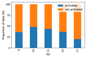
(a) Fera2015

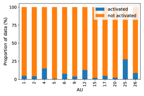
(b) DISFA

Figure 8: Facial action unit (AU) label distribution for FERA2015 and DISFA with respect to the amount of data instances with certain AU being activated or not.

For facial action unit recognition, we applied iterative label-balanced batches to the training to deal with imbalanced datasets. Further, similar to [32] we also used a two phase training scheme.

Two-phase semi-supervised optimization We first trained DISFA and FERA2015 in an unsupervised fashion without any labels involved. For unsupervised training, we used the same architectures as for the semi-supervised training. After unsupervised training, we used the pretrained weights of the encoder and decoder for training with labels. During evaluation we observed an improvement in overall performance when the encoder and decoder were already pretrained.

Iterative label-balanced batches One of the difficulties in recognizing facial action units is due to the imbalance in label distribution. AU activation occurs rarely and varies considerably among subjects as visualized in Figure 8. To tackle this challenge, we introduce iterative balanced batches to deal with the data imbalance during training. We generate batches that are balanced with respect to each action unit by undersampling from the majority class. Since the proportion of positive (activated) samples differ with each action unit, we generate balanced batches with respect to each action unit in an iterative manner. A drawback is that we are removing information that may be valuable. This could lead to underfitting and poor generalization to the test set.

Tables VII and VIII show detailed results w.r.t. to F1 score for DISFA and FERA2015. In particular, it shows average F1 scores for individual AUs as well as the overall average F1 score for each model.

AU	Supervised		Semi-supervised
			$p=0.1$		$p=0.25$
	Resnet18	CNN	VampPriorVAE	MixtureCSRAE	VampPriorVAE	MixtureCSRAE
1	2.44	2.13	0.79	3.75	2.52	3.67
2	26.82	2.93	0.88	4.37	3.59	4.75
4	56.66	43.39	13.64	14.69	27.90	29.26
6	35.67	23.60	27.51	32.20	26.26	30.47
9	27.86	21.35	7.28	12.74	15.52	16.39
12	66.82	56.23	54.84	58.81	56.01	60.57
25	88.28	87.63	54.71	57.32	54.49	54.22
26	39.62	35.83	17.39	17.81	16.50	17.46
Avg.	45.76	34.14	22.13	25.21	25.35	27.10

TABLE VII: Average F1 score from subject-independent 3-fold cross validation for DISFA (higher is better).

AU	Supervised		Semi-supervised
			$p=0.1$		$p=0.25$
	Resnet18	CNN	VampPriorVAE	MixtureCSRAE	VampPriorVAE	MixtureCSRAE
6	77.05	72.50	17.17	24.68	25.81	19.30
10	77.86	78.88	34.77	60.46	33.04	39.10
12	85.98	80.59	32.50	36.32	29.39	39.65
14	44.50	53.18	21.60	28.16	26.90	32.08
17	50.30	9.25	3.43	2.41	7.11	9.25
Avg.	67.54	66.01	23.24	30.56	23.07	27.87

TABLE VIII: Average F1 score from subject-independent 3-fold cross validation for FERA2015 (higher is better).

References

- [1] D. P. Kingma and M. Welling, “Auto-encoding variational bayes,” arXiv preprint arXiv:1312.6114, 2013.
- [2] D. J. Rezende, S. Mohamed, and D. Wierstra, “Stochastic backpropagation and approximate inference in deep generative models,” arXiv preprint arXiv:1401.4082, 2014.
- [3] I. Goodfellow, J. Pouget-Abadie, M. Mirza, B. Xu, D. Warde-Farley, S. Ozair, A. Courville, and Y. Bengio, “Generative adversarial nets,” in Advances in neural information processing systems, pp. 2672–2680, 2014.
- [4] A. Radford, L. Metz, and S. Chintala, “Unsupervised representation learning with deep convolutional generative adversarial networks,” arXiv preprint arXiv:1511.06434, 2015.
- [5] A. v. d. Oord, N. Kalchbrenner, and K. Kavukcuoglu, “Pixel recurrent neural networks,” arXiv preprint arXiv:1601.06759, 2016.
- [6] M. Arjovsky, S. Chintala, and L. Bottou, “Wasserstein gan,” arXiv preprint arXiv:1701.07875, 2017.
- [7] X. Chen, D. P. Kingma, T. Salimans, Y. Duan, P. Dhariwal, J. Schulman, I. Sutskever, and P. Abbeel, “Variational lossy autoencoder,” arXiv preprint arXiv:1611.02731, 2016.
- [8] E. Nalisnick, L. Hertel, and P. Smyth, “Approximate inference for deep latent gaussian mixtures,” in NIPS Workshop on Bayesian Deep Learning, vol. 2, 2016.
- [9] E. Nalisnick and P. Smyth, “Stick-breaking variational autoencoders,” in International Conference on Learning Representations (ICLR), 2017.
- [10] D. J. Rezende and S. Mohamed, “Variational inference with normalizing flows,” in Proceedings of the 32nd International Conference on International Conference on Machine Learning-Volume 37, pp. 1530–1538, JMLR. org, 2015.
- [11] I. Higgins, L. Matthey, A. Pal, C. Burgess, X. Glorot, M. Botvinick, S. Mohamed, and A. Lerchner, “beta-vae: Learning basic visual concepts with a constrained variational framework,” International Conference on Learning Representations, 2016.
- [12] T. Salimans, D. Kingma, and M. Welling, “Markov chain monte carlo and variational inference: Bridging the gap,” in International Conference on Machine Learning, pp. 1218–1226, 2015.
- [13] D. Tran, R. Ranganath, and D. M. Blei, “The variational gaussian process,” arXiv preprint arXiv:1511.06499, 2015.
- [14] K. Gregor, F. Besse, D. J. Rezende, I. Danihelka, and D. Wierstra, “Towards conceptual compression,” in Advances In Neural Information Processing Systems, pp. 3549–3557, 2016.
- [15] D. P. Kingma, T. Salimans, R. Jozefowicz, X. Chen, I. Sutskever, and M. Welling, “Improved variational inference with inverse autoregressive flow,” in Advances in neural information processing systems, pp. 4743–4751, 2016.
- [16] J. M. Tomczak and M. Welling, “Improving variational auto-encoders using householder flow,” arXiv preprint arXiv:1611.09630, 2016.
- [17] R. van den Berg, L. Hasenclever, J. M. Tomczak, and M. Welling, “Sylvester normalizing flows for variational inference,” arXiv preprint arXiv:1803.05649, 2018.
- [18] M. Johnson, D. K. Duvenaud, A. Wiltschko, R. P. Adams, and S. R. Datta, “Composing graphical models with neural networks for structured representations and fast inference,” in Advances in neural information processing systems, pp. 2946–2954, 2016.
- [19] M. D. Hoffman and M. J. Johnson, “Elbo surgery: yet another way to carve up the variational evidence lower bound,” in Workshop in Advances in Approximate Bayesian Inference, NIPS, 2016.
- [20] N. Dilokthanakul, P. A. Mediano, M. Garnelo, M. C. Lee, H. Salimbeni, K. Arulkumaran, and M. Shanahan, “Deep unsupervised clustering with gaussian mixture variational autoencoders,” arXiv preprint arXiv:1611.02648, 2016.
- [21] Y. Zheng, H. Tan, B. Tang, H. Zhou, et al., “Variational deep embedding: A generative approach to clustering,” arXiv preprint, 2016.
- [22] A. Kucukelbir, R. Ranganath, A. Gelman, and D. Blei, “Automatic variational inference in stan,” in Advances in neural information processing systems, pp. 568–576, 2015.
- [23] M. Kuznetsov, D. Polykovskiy, D. P. Vetrov, and A. Zhebrak, “A prior of a googol gaussians: a tensor ring induced prior for generative models,” in Advances in Neural Information Processing Systems, pp. 4104–4114, 2019.
- [24] P. Ghosh, M. S. Sajjadi, A. Vergari, M. Black, and B. Schölkopf, “From variational to deterministic autoencoders,” arXiv preprint arXiv:1903.12436, 2019.
- [25] J. C. Principe, Information theoretic learning: Renyi’s entropy and kernel perspectives. Springer Science & Business Media, 2010.
- [26] K. Kampa, E. Hasanbelliu, and J. C. Principe, “Closed-form cauchy-schwarz pdf divergence for mixture of gaussians,” in Neural Networks (IJCNN), The 2011 International Joint Conference on, pp. 2578–2585, Citeseer, 2011.
- [27] W. Karush, “Minima of functions of several variables with inequalities as side constraints,” M. Sc. Dissertation. Dept. of Mathematics, Univ. of Chicago, 1939.
- [28] H. Kuhn, A. Tucker, et al., “Nonlinear programming,” in Proceedings of the Second Berkeley Symposium on Mathematical Statistics and Probability, The Regents of the University of California, 1951.
- [29] C. P. Burgess, I. Higgins, A. Pal, L. Matthey, N. Watters, G. Desjardins, and A. Lerchner, “Understanding disentangling in -vae,” arXiv preprint arXiv:1804.03599, 2018.
- [30] A. Alemi, B. Poole, I. Fischer, J. Dillon, R. A. Saurous, and K. Murphy, “Fixing a broken elbo,” in International Conference on Machine Learning, pp. 159–168, 2018.
- [31] J. Tomczak and M. Welling, “Vae with a vampprior,” in International Conference on Artificial Intelligence and Statistics, pp. 1214–1223, 2018.
- [32] D. P. Kingma, S. Mohamed, D. J. Rezende, and M. Welling, “Semi-supervised learning with deep generative models,” in Advances in Neural Information Processing Systems 27: Annual Conference on Neural Information Processing Systems 2014, December 8-13 2014, Montreal, Quebec, Canada (Z. Ghahramani, M. Welling, C. Cortes, N. D. Lawrence, and K. Q. Weinberger, eds.), pp. 3581–3589, 2014.
- [33] E. Jang, S. Gu, and B. Poole, “Categorical reparameterization with gumbel-softmax,” in 5th International Conference on Learning Representations, ICLR 2017, Toulon, France, April 24-26, 2017, Conference Track Proceedings, OpenReview.net, 2017.
- [34] H. Larochelle and I. Murray, “The neural autoregressive distribution estimator,” in Proceedings of the Fourteenth International Conference on Artificial Intelligence and Statistics, pp. 29–37, 2011.
- [35] R. Salakhutdinov and I. Murray, “On the quantitative analysis of deep belief networks,” in Proceedings of the 25th international conference on Machine learning, pp. 872–879, ACM, 2008.
- [36] B. M. Lake, R. Salakhutdinov, and J. B. Tenenbaum, “Human-level concept learning through probabilistic program induction,” Science, vol. 350, no. 6266, pp. 1332–1338, 2015.
- [37] B. Marlin, K. Swersky, B. Chen, and N. Freitas, “Inductive principles for restricted boltzmann machine learning,” in Proceedings of the Thirteenth International Conference on Artificial Intelligence and Statistics, pp. 509–516, 2010.
- [38] A. Krizhevsky and G. Hinton, “Learning multiple layers of features from tiny images,” tech. rep., Citeseer, 2009.
- [39] S. M. Mavadati, M. H. Mahoor, K. Bartlett, P. Trinh, and J. F. Cohn, “Disfa: A spontaneous facial action intensity database,” IEEE Transactions on Affective Computing, vol. 4, no. 2, pp. 151–160, 2013.
- [40] M. F. Valstar, T. Almaev, J. M. Girard, G. McKeown, M. Mehu, L. Yin, M. Pantic, and J. F. Cohn, “Fera 2015-second facial expression recognition and analysis challenge,” in 2015 11th IEEE International Conference and Workshops on Automatic Face and Gesture Recognition (FG), vol. 6, pp. 1–8, IEEE, 2015.
- [41] A. van den Oord, O. Vinyals, et al., “Neural discrete representation learning,” in Advances in Neural Information Processing Systems, pp. 6306–6315, 2017.
- [42] X. Glorot and Y. Bengio, “Understanding the difficulty of training deep feedforward neural networks,” in Proceedings of the thirteenth international conference on artificial intelligence and statistics, pp. 249–256, 2010.
- [43] D. Kingma and J. B. Adam, “A method for stochastic optimization,” in International Conference on Learning Representations (ICLR), vol. 5, 2015.
- [44] S. R. Bowman, L. Vilnis, O. Vinyals, A. M. Dai, R. Jozefowicz, and S. Bengio, “Generating sentences from a continuous space,” arXiv preprint arXiv:1511.06349, 2015.
- [45] L. Theis, A. van den Oord, and M. Bethge, “A note on the evaluation of generative models,” in International Conference on Learning Representations (ICLR 2016), pp. 1–10, 2016.
- [46] Y. Burda, R. Grosse, and R. Salakhutdinov, “Importance weighted autoencoders,” arXiv preprint arXiv:1509.00519, 2015.
- [47] X. Zhang, L. Yin, J. F. Cohn, S. J. Canavan, M. Reale, A. Horowitz, P. Liu, and J. M. Girard, “Bp4d-spontaneous: a high-resolution spontaneous 3d dynamic facial expression database,” Image Vis. Comput., vol. 32, no. 10, pp. 692–706, 2014.
- [48] R. Ekman, What the face reveals: Basic and applied studies of spontaneous expression using the Facial Action Coding System (FACS). Oxford University Press, USA, 1997.
- [49] R. S. Feldman, L. Jenkins, and O. Popoola, “Detection of deception in adults and children via facial expressions,” Child development, pp. 350–355, 1979.
- [50] P. K. Rubenstein, B. Schoelkopf, and I. Tolstikhin, “On the latent space of wasserstein auto-encoders,” arXiv preprint arXiv:1802.03761, 2018.
- [51] X. Niu, H. Han, J. Zeng, X. Sun, S. Shan, Y. Huang, S. Yang, and X. Chen, “Automatic engagement prediction with gap feature,” in Proceedings of the 20th ACM International Conference on Multimodal Interaction, pp. 599–603, 2018.
- [52] K. He, X. Zhang, S. Ren, and J. Sun, “Deep residual learning for image recognition,” in Proceedings of the IEEE conference on computer vision and pattern recognition, pp. 770–778, 2016.
- [53] L. Maaløe, M. Fraccaro, V. Liévin, and O. Winther, “Biva: A very deep hierarchy of latent variables for generative modeling,” in Advances in neural information processing systems, pp. 6551–6562, 2019.
- [54] A. Vahdat and J. Kautz, “Nvae: A deep hierarchical variational autoencoder,” Advances in Neural Information Processing Systems, vol. 33, 2020.
- [55] S. Zhao, J. Song, and S. Ermon, “Towards deeper understanding of variational autoencoding models,” arXiv preprint arXiv:1702.08658, 2017.
- [56] D. J. Rezende and F. Viola, “Taming vaes,” arXiv preprint arXiv:1810.00597, 2018.
- [57] B. Dai and D. Wipf, “Diagnosing and enhancing vae models,” in International Conference on Learning Representations, 2018.
- [58] A. Makhzani, J. Shlens, N. Jaitly, I. Goodfellow, and B. Frey, “Adversarial autoencoders,” arXiv preprint arXiv:1511.05644, 2015.
- [59] I. Tolstikhin, O. Bousquet, S. Gelly, and B. Schoelkopf, “Wasserstein auto-encoders,” arXiv preprint arXiv:1711.01558, 2017.
- [60] J. Zeng, W. Chu, F. D. la Torre, J. F. Cohn, and Z. Xiong, “Confidence preserving machine for facial action unit detection,” in 2015 IEEE International Conference on Computer Vision, ICCV 2015, Santiago, Chile, December 7-13, 2015, pp. 3622–3630, IEEE Computer Society, 2015.
- [61] K. Zhao, W. Chu, F. D. la Torre, J. F. Cohn, and H. Zhang, “Joint patch and multi-label learning for facial action unit detection,” in IEEE Conference on Computer Vision and Pattern Recognition, CVPR 2015, Boston, MA, USA, June 7-12, 2015, pp. 2207–2216, IEEE Computer Society, 2015.