Eigenvalues of the truncated Helmholtz solution operator under strong trapping
Abstract
For the Helmholtz equation posed in the exterior of a Dirichlet obstacle, we prove that if there exists a family of quasimodes (as is the case when the exterior of the obstacle has stable trapped rays), then there exist near-zero eigenvalues of the standard variational formulation of the exterior Dirichlet problem (recall that this formulation involves truncating the exterior domain and applying the exterior Dirichlet-to-Neumann map on the truncation boundary).
Our motivation for proving this result is that a) the finite-element method for computing approximations to solutions of the Helmholtz equation is based on the standard variational formulation, and b) the location of eigenvalues, and especially near-zero ones, plays a key role in understanding how iterative solvers such as the generalised minimum residual method (GMRES) behave when used to solve linear systems, in particular those arising from the finite-element method. The result proved in this paper is thus the first step towards rigorously understanding how GMRES behaves when applied to discretisations of high-frequency Helmholtz problems under strong trapping (the subject of the companion paper [MGSS21]).
Keywords.
Helmholtz equation, trapping, quasimodes, eigenvalues, resonances, semiclassical analysis.
AMS subject classifications.
35J05, 35P15, 35B34, 35P25.
1 Introduction
1.1 Preliminary definitions
Let be a bounded open set such that its open complement is connected. Let , where the subscript stands for “Dirichlet”. Let be another bounded open set with connected open complement and such that , where denotes the convex hull and denotes compact containment. Let , and , where the subscript stands for “truncated”. We assume throughout that and are both . Let and denote the Dirichlet traces on and respectively, and let and denote the respective Neumann traces, where the normal vector points out of on both and . Let
Let be the Dirichlet-to-Neumann map for the equation posed in the exterior of with the Sommerfeld radiation condition
| (1.1) |
as , uniformly in . We say that a function satisfying (1.1) is -outgoing. When , for some , the definition of in terms of Hankel functions and polar coordinates (when )/spherical polar coordinates (when ) is given in, e.g., [MS10, Equations 3.7 and 3.10].
Definition 1.1 (Eigenvalues of the truncated exterior Dirichlet problem).
We say is an eigenvalue of the truncated exterior Dirichlet problem at frequency , with corresponding eigenfunction , if and satisfies
Definition 1.2 (Quasimodes).
A family of quasimodes of quality is a sequence such that the frequencies as and there is a compact subset such that, for all , ,
Remark 1.3.
By [Bur98, Theorem 2], we can assume that there exist such that .
Definition 1.4 (Quasimodes with multiplicity).
Let be a quasimode with quality and let be such that and . Define
We say has multiplicity in the window if
We assume throughout that the quality, , of a quasimode is a decreasing function of ; this can always be arranged by replacing by .
We use the notation that as if, given , there exists and such that for all , i.e. decreases superalgebraically in .
1.2 The main results
Theorem 1.5 (From quasimodes to eigenvalues).
Let . Suppose there exists a family of quasimodes of quality with
Then there exists (depending on ) such that, if is such that , then there exists an eigenvalue of the truncated exterior Dirichlet problem at frequency satisfying
We now give three specific cases when the assumptions of Theorem 1.5 hold. The first two cases are via the quasimode constructions of [BCWG+11, Theorem 2.8, Equations 2.20 and 2.21] and [CP02, Theorem 1] for obstacles whose exteriors support elliptic-trapped rays. The third case is via the “resonances to quasimodes” result of [Ste00, Theorem 1]; recall that the resonances of the exterior Dirichlet problem are the poles of the meromorphic continuation of the solution operator from to ; see, e.g., [DZ19, Theorem 4.4. and Definition 4.6].
Lemma 1.6 (Specific cases when the assumptions of Theorem 1.5 hold).
(i) Let . Given , let
| (1.2) |
If coincides with the boundary of in the neighborhoods of the points , and if contains the convex hull of these neighbourhoods, then the assumptions of Theorem 1.5 hold with
for some (independent of ).*** In [BCWG+11, Theorem 2.8], is assumed to contain the whole ellipse . However, inspecting the proof, we see that the result remains unchanged if is replaced with the convex hull of the neighbourhoods of . Indeed, the idea of the proof is to consider a family of eigenfunctions of the ellipse localising around the periodic orbit .
(ii) Suppose , , and contains an elliptic-trapped ray such that (a) is analytic in a neighbourhood of the ray and (b) the ray satisfies the stability condition [CP02, (H1)]. If when and when , then the assumptions of Theorem 1.5 hold with
for some (independent of ).
(iii) Suppose there exists a sequence of resonances of the exterior Dirichlet problem with
| (1.3) |
Then there exists a family of quasimodes of quality and thus the assumptions of Theorem 1.5 hold.
Remark 1.7 (Resonances quasimodes eigenvalues).
Part (iii) of Lemma 1.6 is the “resonances to quasimodes” result of [Ste00, Theorem 1]. The converse implication, i.e. that a family of quasimodes of quality implies a sequence of resonances satisfying (1.3), was proved in [TZ98], [Ste99] (following [SV95, SV96]), see also [DZ19, Theorem 7.6]. Therefore the “quasimodes to eigenvalues” result of Theorem 1.5 is equivalent to a “resonances to eigenvalues” result. In fact, in Appendix A we show that the existence of eigenvalues implies the existence of quasimodes of quality . We therefore have that resonances quasimodes eigenvalues.
With the set of eigenvalues, counting multiplicities, of the truncated exterior Dirichlet problem at frequency (with depending continuously on for each ), let
| (1.4) |
is therefore the counting function of the eigenvalues, , that pass through a rectangle next to zero in as varies in the interval ; see Figure 1.1. †††In Figure 1.1 we have drawn the paths of the eigenvalues as arbitrary curves. We see later in Figure 1.7 an example where the paths appear to be horizontal lines; this is consistent with the intuition that eigenvalues should be shifted resonances.
Theorem 1.8 (From quasimodes to eigenvalues, with multiplicities).
Let such that there is satisfying . Suppose there exists a family of quasimodes of quality and multiplicity in the window (in the sense of Definition 1.4). If is such that, for some ,
then there exists such that if ,
Observe that if , then (up to algebraic powers of ) Theorem 1.8 reduces to Theorem 1.5, except that now multiplicities are counted; therefore the “quasimodes to eigenvalues” result holds with multiplicities (just as the “quasimodes to resonances” result of [Ste99] includes multiplicities).
Remark.
The reason why both the constant in Theorem 1.5 and the exponent in the bound on the quality Theorem 1.8 depend on is because the right-hand side of the bound (1.15) below on the solution operator of the truncated problem depends on , which in turn comes from the fact that the trace-class norm of compactly-supported pseudodifferential operators depends on .
1.3 Numerical experiments illustrating the main results
Description of the obstacles .
In this section, is one of the two “horseshoe-shaped” 2-d domains shown in Figure 1.2. We define the small cavity as the region between the two elliptic arcs
this corresponds to the interior of the solid lines in Figure 1.2. We define the large cavity as the region between the two arcs now with . (Note that our small cavity is the same as the cavity considered in the numerical experiments in [BCWG+11, Section IV].) Recall that Theorems 1.5 and 1.8 require to be smooth, and thus these results do not strictly apply to the small and large cavities; however they do apply to smoothed versions of these.
For both the small and large cavities, coincides with the boundary of the ellipse (1.2) with and in the neighbourhood of its minor axis. Part (i) of Lemma 1.6 (i.e., the results of [BCWG+11]) then implies that there exist quasimodes with exponentially-small quality.
We choose these particular because we can compute the frequencies in the quasimode. Indeed, the functions in the quasimode construction in [BCWG+11] are based on the family of eigenfunctions of the ellipse localising around the periodic orbit ; when the eigenfunctions are sufficiently localised, the eigenfunctions multiplied by a suitable cut-off function form a quasimode, with frequencies equal to the square roots of eigenvalues of the ellipse. By separation of variables, can be expressed as the solution of a multiparametric spectral problem involving Mathieu functions; see see [BCWG+11, Appendix A] and [MGSS21, Appendix E].
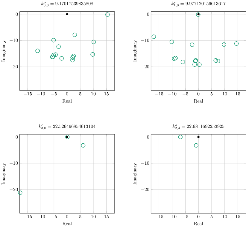
When giving specific values of below, we use the notation from [BCWG+11, Appendix A] and [MGSS21, Appendix E] that and are the frequencies associated with the eigenfunctions of the ellipse that are even/odd, respectively, in the angular variable, with zeros in the radial direction (other than at the centre or the boundary) and zeros in the angular variable in the interval .


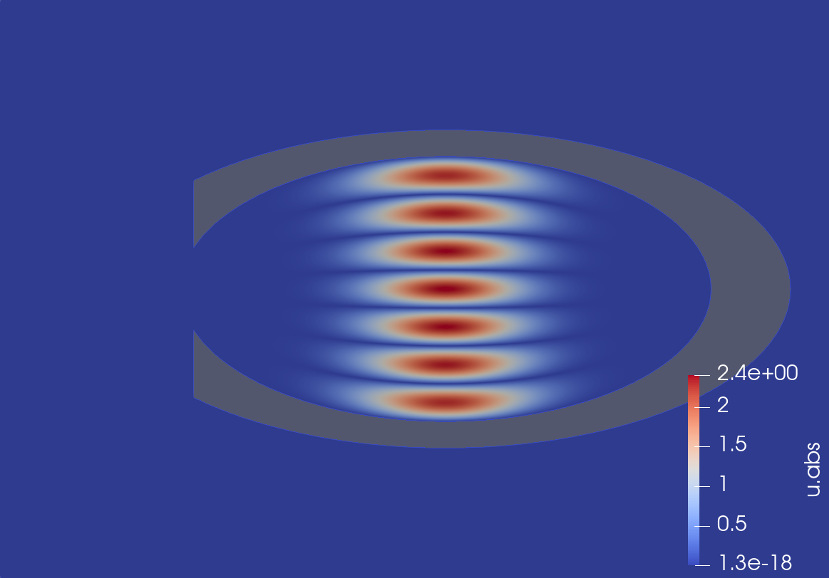
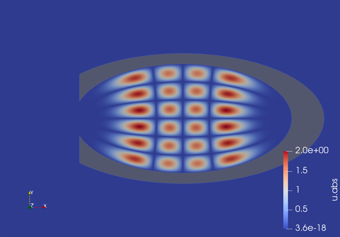
Plots of the eigenvalues and eigenfunctions
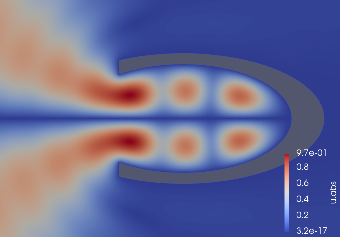
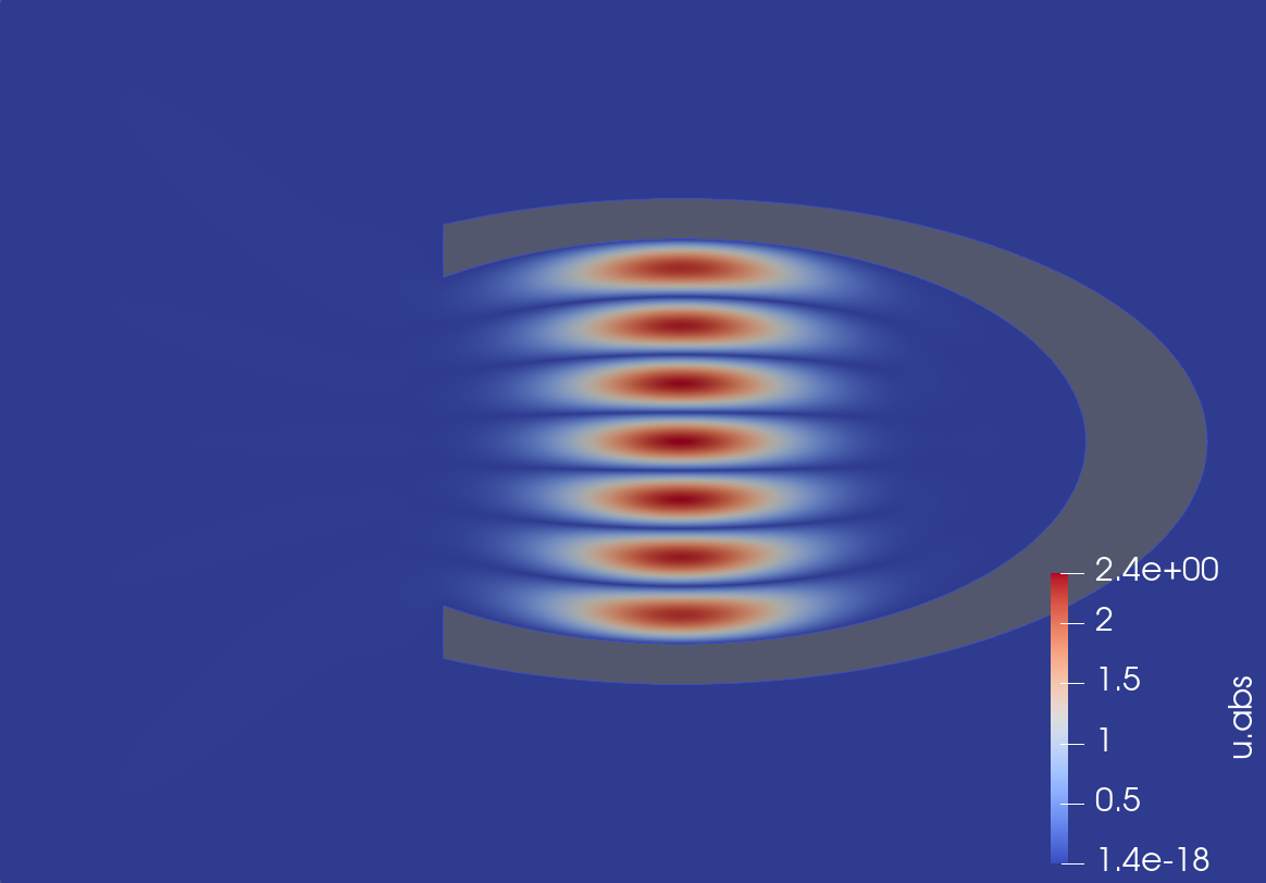
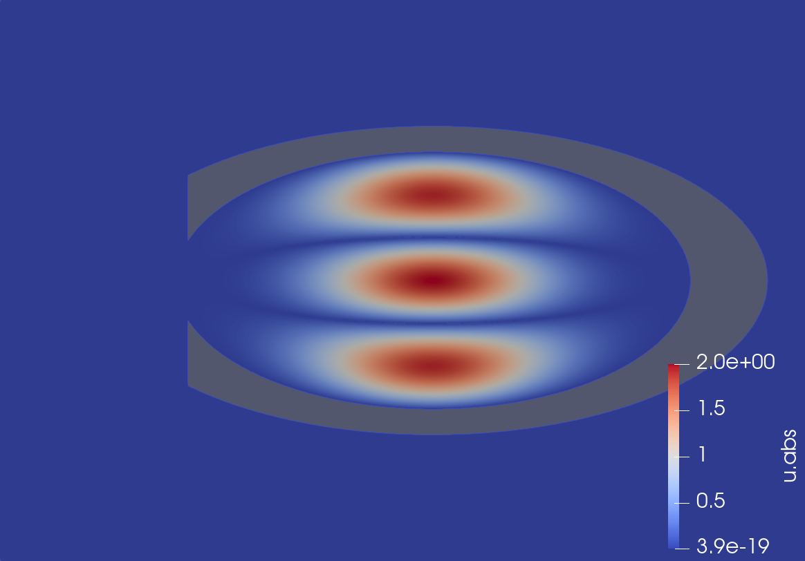
Figures 1.3 and 1.4 plot the near-zero eigenvalues of the truncated exterior Dirichlet problem for the small and large cavity, respectively, at frequencies corresponding to eigenvalues of the ellipse. Figures 1.5 and 1.6 plot the corresponding eigenfunctions. In all these figures .
Figure 1.4 shows that the large cavity has an eigenvalue very close to zero at each of the four frequencies considered, qualitatively illustrating Theorem 1.5. In contrast, Figure 1.3 shows that the small cavity only has an eigenvalue very close to zero at the frequencies and (top right and bottom left in the figures) and not at and (top left and bottom right). The reason for this is clear from the plots of the eigenfunctions of the truncated exterior Dirichlet problem: looking at Figure 1.5, we see that at and the eigenfunctions are not well localised around the minor axis of the ellipse to be inside the small cavity – in the top left and bottom right of Figure 1.5 we see them “leaking out” of the small cavity. However, looking at Figure 1.6, we see that the corresponding eigenfunctions are localised sufficiently to be inside the large cavity, and thus generate an eigenvalue very close to zero. In these plots, the eigenfunctions are normalised so that their norm equals one.
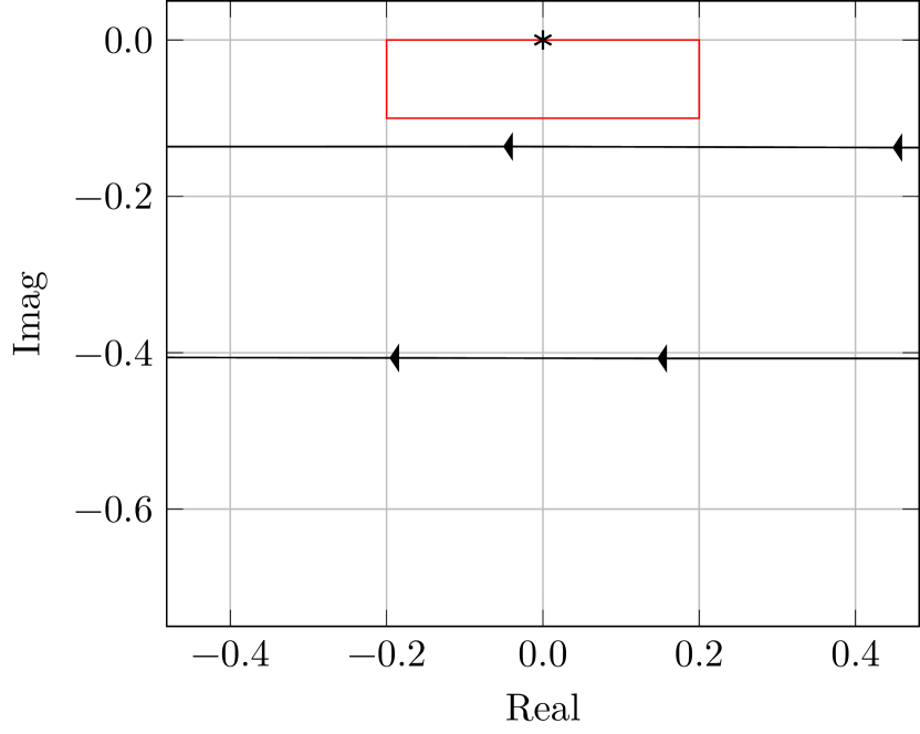
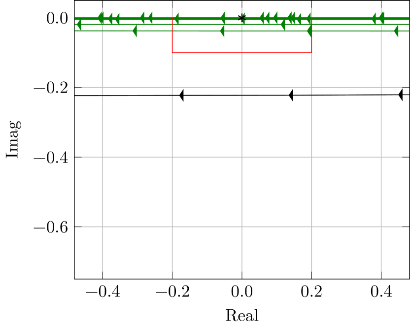
Figure 1.7 plots the trajectories of the near-zero eigenvalues as functions of for both the small cavity (left plot) and large cavity (right plot) for , with the spectra computed every . For Figure 1.7, ; this change (compared to for the earlier figures) is to reduce the cost of each eigenvalue solve, because each of the two plots in Figure 1.7 requires such solves. Since we use the exact (up to discretisation error) Dirichlet-to-Neumann map on , we expect there to be no difference between choosing and (in particular Figures 1.3 and 1.4 are unchanged when is changed from to ).
The eigenvalues that enter the red rectangle in Figure 1.7 are coloured green; these are members of , where is defined by (1.4). Similar to the eigenvalues plots in Figures 1.3 and 1.4, Figure 1.7 shows that the large cavity has more near-zero eigenvalues for the range of considered than the small cavity. This is expected since a larger number of the eigenfunctions of the ellipse are localized in the large cavity than in the small cavity.
How the eigenvalues and eigenfunctions were computed.
Definition 1.1 (of the eigenvalues of the truncated Dirichlet problem) implies that if is an eigenvalue at frequency , and with corresponding eigenfunction , then
| (1.5) |
where the sesquilinear form is that appearing in the standard variational (i.e. weak) formulation of the Helmholtz exterior Dirichlet problem.
Definition 1.9 (Variational formulation of Helmholtz exterior Dirichlet problem).
Given , as above, and , let be the solution of the variational problem
| (1.6) |
where
| (1.7) |
where denotes the duality pairing on that is linear in the first argument and antilinear in the second.
The figures above were created by solving the eigenvalue problem (1.5) using the finite-element method with continuous piecewise-linear elements (i.e. the polynomial degree, , equals one) and meshwidth , equal . The Dirichlet-to-Neumann map, , in was computed using boundary integral equations – see Appendix B for details. The accuracy, uniform in frequency, of the finite-element applied the variational problem (1.6) with and sufficiently small has been known empirically for a long time, and was recently proved in [LSW19] for the case when the Dirichlet-to-Neumann map is realised exactly.
Since computing the Dirichlet-to-Neumann map is relatively expensive, in practice one often approximates it using a perfectly-matched layer (PML) or an absorbing boundary condition (such as the impedance boundary condition). The plots of the eigenfunctions and near-zero eigenvalues of the corresponding truncated exterior Dirichlet problems are very similar to those above; this too is expected since the quasimode is supported in a neighbourhood of the obstacle.
1.4 Implications of the main results for numerical analysis of the Helmholtz exterior Dirichlet problem
Theorems 1.5 and 1.8 are the first step towards rigorously understanding how iterative solvers such as the generalised minimum residual method (GMRES) behave when applied to discretisations of high-frequency Helmholtz problems under strong trapping (the subject of the companion paper [MGSS21]). We now explain this in more detail.
As we saw in (1.5), the eigenvalues of truncated exterior Dirichlet problem (in sense of Definition 1.1) correspond to eigenvalues of sesquilinear form of standard variational formulation (Definition 1.9). The standard variational formulation is the basis of the finite-element method for computing approximations to the solution of the variational problem (1.6). Indeed, the finite-element method consists of choosing a piecewise-polynomial subspace of and solving the variational problem (1.6) in this subspace.
A very popular way of solving the linear systems resulting from the finite-element method applied to the Helmholtz scattering problems is via iterative solvers such as GMRES [SS86]; this choice is made because the linear systems are (i) large and (ii) non-self-adjoint. Regarding (i): the systems are large since the number of degrees of freedom must be to resolve the oscillations in the solution, see, e.g., the literature review in [LSW19, §1.1]. Regarding (ii): non-self-adjointness of the linear systems arises directly from the non-self-adjointness of the underlying Helmholtz scattering problem; GMRES is applicable to such systems, unlike the conjugate gradient method.
There is currently large research interest in understanding how iterative methods behave when applied to Helmholtz linear systems, and in designing good preconditioners for these linear systems; see the literature reviews [Erl08, EG12, GZ19], [GSZ20, §1.3].
The location of eigenvalues, especially near-zero ones, is crucial in understanding the behaviour of iterative methods. In the Helmholtz context, eigenvalue analyses of iterative methods applied to nontrapping problems include, for finite-element discretisations, [EO99, EEO01, EVO04, VGEV07, EG12, VG14, CG17, LXSdH20], and, for boundary-element discretisations, [CH01, DDL13, CDLL17].
The paper [MGSS21] analyses GMRES applied to discretisations of Helmholtz problems with strong trapping, using the “cluster plus outliers” GMRES convergence theory from [CIKM96] (with this idea arising in the context of the conjugate gradient method [Jen77] and used subsequently in, e.g., [ESW02]). The paper [MGSS21] obtains bounds on how the number of GMRES iterations depends on the frequency, under various assumptions about the eigenvalues. In particular, Theorem 1.5 rigorously justifies [MGSS21, Observation O2(b)] for the standard variational formulation of the truncated exterior Dirichlet problem. We highlight that, although the results in [MGSS21] are about unpreconditioned systems, they give insight into the design of preconditioners. Indeed, a successful preconditioner for Helmholtz problems with strong trapping will need to specifically deal with the near-zero eigenvalues created by trapping. Theorem 1.5 and 1.8 give information about the location and multiplicities of these eigenvalues, and [MGSS21] shows how these locations and multiplicities affect GMRES.
1.5 The ideas behind the proof of Theorem 1.5
Semiclassical notation.
Instead of working with the parameter and being interested in the large- limit, the semiclassical literature usually works with a parameter and is interested in the small- limit. So that we can easily recall results from this literature, we also work with the small parameter , but to avoid a notational clash with the meshwidth of the FEM, we let (the notation comes from the fact that the semiclassical parameter is sometimes related to Planck’s constant, which is written as ; see, e.g., [Zwo12, §1.2]). Theorem 1.5 is then restated in semiclassical notation as Theorem 2.2 below.
The solution operator of the truncated problem.
Let be the solution operator for the truncated problem
| (1.8) |
that is, satisfies
Note that, at this point, it is not clear that the problem (1.8) is well posed and that the family of operators is well defined. We address this in Lemma 1.10 below.
We study by relating it to the solution operator of a more-standard scattering problem. Namely, let with , and consider the problem
| (1.9) |
By, e.g., [DZ19, Chapter 4], the inverse of (1.9) is a meromorphic family of operators (for when is odd or in the logarithmic cover of when is even) with finite-rank poles satisfying
| (1.10) |
Observe that, although both and depend on , we omit this dependence in the notation to keep expressions compact.
The following two lemmas (proved in §2.2) relate and and then characterise the eigenvalues of the truncated exterior Dirichlet problem as poles of as a function of .
We use three indicator functions: denotes the function in that is one on and zero otherwise, denotes the restriction operator , and denotes the extension-by-zero operator .
Lemma 1.10.
Define
| (1.11) |
Then
| (1.12) |
and thus is a meromorphic family of operators in for when is odd and in the logarithmic cover of when is even.
Lemma 1.11.
For , is a meromorphic family of operators with finite rank poles.
Corollary 1.12.
If is a pole of , then is an eigenvalue of the truncated exterior Dirichlet problem (in the sense of Definition 1.1).
The key point is that we are interested in as a meromorphic family in the variable , in contrast to the more-familiar study of as a meromorphic family in the variable .
Recap of “from quasimodes to resonances”.
Recall that resonances of are defined as poles of the meromorphic continuation of into , see [DZ19, §4.2, §7.2]. The “quasimodes to resonances” argument of [TZ98] (following [SV95, SV96]; see also [DZ19, Theorem 7.6]) shows that existence of quasimodes (as in Definition 1.2) implies existence of resonances close to the real axis; the additional arguments in [Ste99] then prove the corresponding result with multiplicities.
From quasimodes to eigenvalues.
Theorems 1.5 and 1.8 are proved using the same ideas as in the quasimodes to resonances arguments, except that now we work in the complex -plane (with real ) instead of the complex -plane. The analogue of the bounds (1.13) and (1.14) are given in the following lemma.
Lemma 1.13 (Bounds on ).
Let and let be the poles of (as a meromorphic function of ). Then there exist such that for all , and ,
| (1.15) |
Furthermore, there exists such that
| (1.16) |
where .
The bound (1.15) is proved by finding a parametrix for (i.e. an approximation to ) via a boundary complex absorbing potential. While parametrices based on complex absorption are often used in scattering theory (see, e.g., [DZ16, DG17] [DZ19, Theorem 7.4]), parametrices based on boundary complex absorption appear to be new in the literature. One of the main features of the argument below is that it relies on a comparison of the (in principle, trapping) billiard flow with the non-trapping free flow to obtain estimates on the parametrix. A similar argument should work for boundaries in any non-trapping background.
We also highlight that, while we consider the scattering by Dirichlet obstacles in this paper and therefore must use boundary complex absorption, smooth compactly-supported perturbations of , e.g. metric perturbations or semiclassical Schrödinger operators, can be handled similarly. Indeed, for these problems, the parametrix based on boundary absorption could be replaced by one based on simpler complex absorbing potentials.
1.6 Outline of the rest of the paper
In §2 we prove Lemmas 1.10 and 1.11 and then collect preliminary results about the generalized bicharacteristic flow (§2.4), the geometry of trapping (§2.5), complex scaling (§2.6), and defect measures (§2.8). In §3 we find a parametrix for via a boundary complex absorbing potential. In §4 we prove Lemma 1.13. In §5 we prove Theorems 1.5 and 1.8 using Lemma 1.13 and the semiclassical maximum principle.
2 Preliminary results
2.1 Restatement of Theorems 1.5 and 1.8 in semiclassical notation
Definition 2.1 (Quasimodes in notation).
A family of quasimodes of quality is a sequence such that as and there is a compact subset such that, for all , ,
Let
| (2.1) |
Remark 1.3 implies that we can assume that there exist such that
| (2.2) |
Theorem 1.5 is then equivalent to the following result in the sense that the following result holds if and only if Theorem 1.5 holds with .
Theorem 2.2 (Analogue of Theorem 1.5 in notation).
Let . Suppose there exists a family of quasimodes in the sense of Definition 2.1 such that the quality satisfies
| (2.3) |
Then there exists (depending on ) such that, if is such that then there exists and with
| (2.4) |
Definition 2.3 (Quasimodes with multiplicity in notation).
Let be two functions of . A family of quasimodes of quality and multiplicity in the window is a sequence such that as and for every there exist with
and for all and , where .
With the set of poles of counting multiplicities (with depending continuously on for each ), let
| (2.5) |
is therefore the counting function of the poles of that enter a rectangle next to zero in as varies from to .
Theorem 2.4 (Analogue of Theorem 1.8 in notation).
Let and suppose there exists a family of quasimodes with quality
| (2.6) |
and multiplicity in the window (in the sense of Definition 2.3). If is such that, for some ,
| (2.7) |
then there exists such that if , then
Proof of Theorem 1.8 from Theorem 2.4.
We first show that if there exists a family of quasimodes with multiplicity in the window in notation (i.e. in the sense of Definition 1.4), then there exists a family of quasimodes in notation (in the sense of Definition 2.3).
Without loss of generality, each for some (if necessary by adding a window with ), i.e. given in the index set of the quasimode, there exists such that . We now index the quasimode with the index describing the windows . Let
Then,
where we have used that is a decreasing function of . Therefore, we have shown that there exists a family of quasimodes with multiplicity in the window in notation (i.e. in the sense of Definition 2.3).
2.2 Results about meromorphic continuation
Proof of Lemma 1.10.
Once we show (1.12), the meromorphicity of in follows from the corresponding result for [DZ19, Theorem 4.4].
We first show that the appropriate extension of a solution of (1.8) is a solution of (1.9) with . We then show that the appropriate restriction of the solution of (1.9) with is a solution of (1.8).
Proof of Lemma 1.11.
Since
the definition of (1.11) implies that
| (2.11) |
We now claim that, for any with and on
| (2.12) |
Indeed,
and thus
| (2.13) |
Observe that since is compact, is compact, and the analytic Fredholm theorem [DZ19, Theorem C.8] implies that
| (2.14) |
with finite rank poles.
Now, since , for small enough,
| (2.15) |
However, by (2.14) both the left- and right-hand sides of (2.15) are meromorphic for . Therefore, (2.15) holds for all and hence
| (2.16) |
Using (2.15) and (2.16) in (2.13), we obtain (2.12). Therefore, for on and on , (2.11), (2.12) and (2.15) imply that
Using (2.14) again completes the proof. ∎
With a pole of , let
| (2.17) |
where denotes integration over a circle containing and no other pole of .
The following result then holds by, e.g., [DZ19, Theorem C.9].
Lemma 2.5.
For , is a bounded projection with finite rank.
The next result concerns the singular behaviour of near its poles in , and is analogous to (parts of) [DZ19, Theorem 4.7] concerning the singular behaviour of near its poles in .
Lemma 2.6.
For , if and , then there exists such that
where is holomorphic near .
Proof.
By Lemma 1.11, for , is a meromorphic family of operators (in the sense of [DZ19, Definition C.7]) from and thus there exists , finite-rank operators , , and a family of operators from , holomorphic near , such that
By integrating around and using the residue theorem, we have . Then, with denoting equality up to holomorphic operators,
where we define . Since on , , , and the result follows from density of in . ∎
2.3 The semiclassical maximum principle
The following result is the semiclassical maximum principle of [TZ98, Lemma 2], [TZ00, Lemma 4.2] (see also [DZ19, Lemma 7.7]).
Theorem 2.7 (Semiclassical maximum principle).
Let be an Hilbert space and an holomorphic family of operators in a neighbourhood of
| (2.18) |
where
| (2.19) |
for some and . Suppose that
| (2.20) | ||||
| (2.21) |
Then
| (2.22) |
2.4 The generalized bicharacteristic flow
Recall that
and
We write for the generalized bicharacteristic flow associated to a symbol (see e.g. [Hör85, §24.3]). Since the flow over the interior is generated by the Hamilton vector field , for any symbol ,
| (2.23) |
where denotes the Poisson bracket; see [Zwo12, §2.4].
We primarily consider the case when is the semiclassical principal symbol of the Helmholtz equation, namely . By Hamilton’s equations, away from the boundary of , the corresponding flow satisfies and , and thus, for with away from , for sufficiently small; i.e., the flow has speed two.
We let denote the projection operator onto the spatial variables; i.e.
2.5 Geometry of trapping
Let with and near and define by
so that there is such that for ,
Moreover, note that is compact for every . Next, define the directly escaping sets,
Then,
| (2.24) |
Therefore, as and hence escapes forward/backward in time. This, in particular implies that
| (2.25) |
We now define the outgoing tail , the incoming tail , and the trapped set, by
| (2.26) |
i.e. the outgoing tail is the set of trajectories that do not escape as , the incoming tail is the set of trajectories that do not escape as , and the trapped set is the set of trajectories that do not escape in either time direction.
We now recall some basic properties of and , with these proved in a more general setting in [DZ19, §6.1].
Lemma 2.8.
(i) The sets are closed in and .
(ii) Suppose that with and there are such that . Then .
Proof.
(i) We show that is closed in Suppose that . Then as . In particular, there are such that and . So, applying (2.25) with , we have . Since is open and is continuous we have for all sufficiently close to and hence, by (2.24), . Therefore is closed. By an identical argument and hence are closed.
Now, we show that . Note that . But, and and hence as claimed.
(ii) We prove the result for ; the proof of the other case is similar. Seeking a contradiction, assume that . Then there exists such that and hence, since is continuous, and is open, for large enough, . But then, by (2.24) and (2.25) for . In particular, for large enough,
which contradicts the fact that . ∎
2.6 Complex scaling
We now review the method of complex scaling following [DZ19, §4.5]. We first fix a small angle of scaling, , and the radius, , where the scaling starts; without loss of generality, we assume that . Let satisfy
Then, consider the totally real submanifold (see [DZ19, Definition 4.28])
and note that we identify with its image on . We define the complex scaled operator on by the Dirichlet realization of
where denotes the Laplacian on the round sphere . Note that is a semiclassical differential operator of second order such that on , with principal symbol, , satisfying on and in polar coordinates ,
| (2.27) |
Now, by e.g. [DZ19, Theorems 4.36,4.38], for ,
| (2.28) |
In particular, for , , this implies that
| (2.29) |
Moreover, by [DZ19, Theorem 4.37], has the same poles as and, for with ,
| (2.30) |
2.7 Semiclassical pseudodifferential operators
For simplicity of exposition, we begin by discussing semiclassical pseudodifferential operators on , and then outline below how to extend the results from to a manifold (with these results then applied with or ).
A symbol is a function on that is also allowed to depend on , and thus can be considered as an -dependent family of functions. Such a family , with , is a symbol of order , written as , if for any multiindices
| (2.31) |
where and does not depend on ; see [Zwo12, p. 207], [DZ19, §E.1.2].
For , we define the semiclassical quantisation of , denoted by , by
| (2.32) |
[Zwo12, §4.1] [DZ19, §E.1 (in particular Page 543)]. The integral in (2.32) need not converge, and can be understood either as an oscillatory integral in the sense of [Zwo12, §3.6], [H8̈3, §7.8], or as an iterated integral, with the integration performed first; see [DZ19, Page 543].
Conversely, if can be written in the form above, i. e. with , we say that is a semiclassical pseudo-differential operator of order and we write . We use the notation if ; similarly if . We write .
Let the quotient space be defined by identifying elements of that differ only by an element of . For any , there is a linear, surjective map
called the principal symbol map, such that, for ,
| (2.33) |
see [Zwo12, Page 213], [DZ19, Proposition E.14] (observe that (2.33) implies that ). When applying the map to elements of , we denote it by (i.e. we omit the dependence) and we use to denote one of the representatives in (with the results we use then independent of the choice of representative). Key properties of the principal symbol that we use below is that
| (2.34) |
where (as in §2.4) denotes the Poisson bracket; see [DZ19, Proposition E.17] and [DZ19, Equation E.1.44], [Zwo12, Page 68].
While the definitions above are written for operators on , semiclassical pseudodifferential operators and all of their properties above have analogues on compact manifolds (see e.g. [Zwo12, §14.2], [DZ19, §E.1.7]). Roughly speaking, the class of semiclassical pseudodifferential operators of order on a compact manifold , are operators that, in any local coordinate chart, have kernels of the form (2.32) where the function modulo a remainder operator that has the property
| (2.35) |
We say that an operator satisfying (2.35) is .
Semiclassical pseudodifferential operators on manifolds continue to have a natural principal symbol map
where now is a class of functions on , the cotangent bundle of which satisfy the estimates (2.31). Furthermore, (2.34) holds as before.
Finally, there is a noncanonical quantisation map that satisfies
and for all , there is such that
2.8 Defect measures
We say that a sequence with for all (with independent of ) has defect measure if for all ,
where is defined by (2.32). By, e.g., [Zwo12, Theorem 5.2], is a positive Radon measure on . We say that and have joint defect measure if
| (2.36) |
We usually suppress the in the notation and instead write that has defect measure and and have joint defect measure .
Lemma 2.9.
([Zwo12, Theorem 5.3].) Let and suppose that has defect measure and satisfies
Then, where is the semiclassical principal symbol of .
The following lemma is the defect-measure analogue of the propagation of singularities result [DZ19, Theorem E.47].
Lemma 2.10.
Let with . There exists such that the following holds: suppose that has defect measure and satisfies
where and and have joint defect measure . Then, for all real valued ,
Proof.
Let . Since (by [DZ19, Equation E.1.45]) and thus (by [DZ19, Equation E.1.43]), by the definition of the joint measure (2.36),
| (2.37) |
Since and with and both self-adjoint,
| (2.38) |
where the last line follows from the sharp Garding inequality (see, e.g., [DZ19, Proposition E.32]) and the fact that . By (2.34),
and therefore, since the kernel of is , and, in particular,
| (2.39) |
The lemma follows from combining (2.38) with (2.39) and (2.37), and sending . ∎
Corollary 2.11.
Let and suppose the assumptions of Lemma 2.10 hold and, in addition, . Then, with the bicharacteristic flow corresponding to the symbol , for any ,
| (2.40) |
Corollary 2.11 shows that, under the assumptions of Lemma 2.10, we have information about the defect measures of sets moving forward under the flow.
Proof of Corollary 2.11.
Let By (2.23),
and thus
| (2.41) |
Let be the indicator function of . By approximating by squares of smooth symbols, compactly supported symbols (2.41) holds with . Since the result (2.40) follows. More precisely, we first let open and compact with and choose with on and . The result for open follows by monotonicity of measure from below; the result for general follows by outer regularity of . ∎
We now review some recent results from [GLS21] about defect measures when satisfies the Helmholtz equation. Let be such that .
We use Riemannian/Fermi normal coordinates in which is given by and is . The conormal and cotangent variables are given by . Recall the definition of the hyperbolic set
(where the metric is that induced by ) and the definition of the gliding set
Let and have real-valued principal symbols satisfying
| (2.42) |
where and denotes the norm of in the metric, , induced on from . Let be a solution to
Later we restrict attention to specific and , but we consider more-general operators here because we believe some of our intermediate results (specifically Lemma 3.3) are of independent interest; see [GMS21].
Suppose that has defect measure and and have joint defect measure . On , let be the joint measure associated with the Dirichlet and Neumann traces and be the measure associated with the Neumann trace; see [GLS21, Theorem 2.3]. In what follows, we only use the fact that where is bounded (see [GLS21, Lemma 2.14 and §4]).
With as above, let be the positive measures on , supported in the hyperbolic set , and defined in [GLS21, Lemma 2.9]/[Mil00, Proposition 1.7, Part (ii)].
In the following lemma, denotes the -cotangent bundle to and is defined in local coordinates by (for more details about , see, e.g., [Hör85, Section 18.3], [GSW20, Section 4B]).
Lemma 2.12.
With , , , , , and as above,
-
(i)
-
(ii)
For all ,
-
(iii)
For all ,
(where the integral is understood as the integral of distributions acting on smooth functions).
-
(iv)
On , , where
(2.43)
3 Parametrix for via boundary complex absorption
We now find a parametrix for using a complex absorbing potential on the boundary . We then obtain by perturbation a parametrix for for sufficiently small.
First, let
Then let be an extension operator satisfying
Simple calculation then implies that
| (3.1) |
where is the inverse of (2.28).
Lemma 3.1.
The operator is Fredholm with index zero.
Proof.
Recall that the map (2.28) is Fredholm with index zero. First, note that if , then and in particular, . Therefore, since is Fredholm, is finite dimensional. To see that the cokernel is finite dimensional, define the map
First, observe that this map is well defined since if then there is such that
In particular,
so .
Now, suppose that . Then, there is such that
Therefore,
and is injective. For an injective operator, ; therefore
Since is Fredholm, is Fredholm. To see that has index zero, recall that the index is constant in by, e.g., [DZ19, Theorem C.5], and observe that the formula (3.1) implies that the inverse exists for some . ∎
We now define our complex absorbing operator. Let with on and . It will be convenient to have a specific notation for the Neumann trace with the standard derivative operator replaced by . We therefore let . Let
where with symbol
| (3.2) |
Note that
and hence is a compact perturbation of . Therefore, by Lemma 3.1, is Fredholm with index zero.
Lemma 3.2.
Let be as above and and . Then there exists such that for all ,
| (3.3) |
In particular, since is Fredholm with index zero,
exists and satisfies
| (3.4) |
Observe that the bound (3.4) has the same -dependence as the standard non-trapping resolvent estimate.
Before proving Lemma 3.2 we show how a parametrix for the operator can be expressed in terms of . Let
By Lemma 3.2, the bound (3.4), and inversion by Neumann series, for (where is the constant from Lemma 3.2)
exists and satisfies
| (3.5) |
Next, let
| (3.6) |
If exists, then
where
| (3.7) |
Since is compact, is a meromorphic family of operators by [DZ19, Theorem C.8]. Therefore, for ,
| (3.8) |
Let be the inverse of the map (2.29) with , i.e.
| (3.9) |
Then, for ,
| (3.10) |
which is the required parametrix.
Proof of Lemma 3.2.
Suppose that the estimate (3.3) fails with the left-hand side replaced by , then there are , , and with
and with
In particular, renormalizing , , and ,
and
Now, since , we may rescale to and hence replace by . Note that this rescaling does not cause any issues since Extracting a subsequence, we can assume that has defect measure (see e.g. [Zwo12, Theorem 5.2]) and , and . Since , .
Let with and in a neighborhood of and . We first show that
| (3.11) |
To do this, observe that, by (2.27),
| (3.12) |
Therefore, by ellipticity, for a neighborhood of ,
| (3.13) |
Now, by (3.12) and the definitions of and ,
Therefore, by [Zwo12, Theorem 4.29],
| (3.14) |
But,
| (3.15) |
where we have used that, by direct computation, in the second inequality; (3.11) then follows from combining (3.14) and (3.15).
We now show that . First, observe that
| (3.16) |
Consequently, using (3.13) in (3.16) we find that
Since on , we can now apply Lemma 2.12 (with in that lemma replaced by here) to find that
where we have used (3.11) in the second equality. Moreover,
so that in fact .
We now show that which is a contradiction. To do this, we start by observing that (3.11) implies that . In fact, by Lemma 2.9, , and therefore, .
Now, Lemma 2.12, along with Lemma 2.10 together with the fact that , allows us to propagate forward along the generalized bicharacteristic flow (in the sense of Corollary 2.11), but not backward. In particular, since , this implies that . Indeed, suppose that is compact and . Then, by the definition of (2.26), for each there is such that . Hence, by (2.24) for , and by continuity of , there is a neighborhood of such that for . In particular, by compactness of , there is such that . By compactness of in the variable and (2.40), there is such that . Now, by Lemma 2.8, is closed and hence we may write with compact. In particular, by monotonicity from below.
Next, note that since on ,
by Lemma 2.9. In particular, by the definition of ,
To complete the proof, we need to show that in fact . This is where the boundary term is used.
We claim there are such that
| (3.17) |
for all . Once this is done, we have that . To see this, observe that if , then by induction . Taking , we have , which is a contradiction to .
We now prove (3.17). First, note that the statement is empty if . Therefore, we can assume that . Since , we assume that ; since is closed, we can assume that is compact. Now, by (2.24), (2.25), and (2.26),
Therefore, increasing by , we may assume that .
Letting and and recalling (3.2), we see that and satisfy (2.42). Therefore, the proof of (3.17) is completed by the next lemma.
Lemma 3.3.
Proof.
We claim that there are such that for all with .
| (3.18) |
where is the orthogonal projection and is given by (2.43).
Once (3.18) is proved, we claim that Lemma 2.12 implies (3.17) with . Indeed, suppose that (3.18) holds and that , and is closed. Then, let with on and
| (3.19) |
Now, let on with . Then,
with and hence by Lemma 2.12
But, by (3.19), on for . In particular, for
Finally, since is closed we may approximate by smooth, compactly supported functions to obtain
| (3.20) |
Now, to study (3.20), we first assume that and are such that for all and , does not lie in the glancing region () and each trajectory intersects exactly once and does so for . Shrinking the support of further if necessary, we can find transverse to the vector field such that
are smooth coordinates and is in the image of for all . Then, (3.20) reads
Now, arguing as in [GLS21, Lemma 2.16], we obtain that and hence,
Therefore
where this last equality comes from evaluating the integral using the fact that is well-defined (since each trajectory intersects exactly once).
so that, in particular, trajectories from do not intersect the hyperbolic set. In this case, (3.20) implies that
| (3.21) |
In particular, shrinking if necessary, we may choose transverse to and work in coordinates
In these coordinates, (3.21) implies that is absolutely continuous with respect to in the sense that there is a family of measures, on such that and . Moreover,
In particular,
Putting everything together, we have for all and ,
as claimed.
Therefore, it is enough to prove (3.18). Seeking a contradiction, we assume that for every and there is with such that
| (3.22) |
Note that since both terms are non-positive (since and ), this implies that each term is .
Now, if for , then, since the flow in is given by the flow of the vector field
(see [Hör85, Def. 24.3.6]), we obtain, using that on (since ).
where both here and in the rest of this proof we write if for some depending only on and . On the other hand, if for , and has exactly one intersection with , then
where is measured at the point of reflection. All together, since on , and thus there is such that
we obtain from (3.22) that
Therefore, choosing , and small enough, we obtain
which is a contradiction to . ∎
We have therefore proved that
| (3.23) |
where here, and in the rest of the proof, denotes a constant, independent of , , and , whose value may change from line to line. To complete the proof of Lemma 3.2, we now need to obtain a bound on the norm of , as opposed to just the norm in (3.23). By a standard elliptic parametrix construction, for supported away from , we have
by (3.23). Finally, using the trace estimate from [GLS21, Corollary 4.2] we have for with ,
Elliptic regularity for the Laplacian then implies that
where we have used (3.23). Combining the bounds on , , and , we obtain (3.4). ∎
4 Proof of Lemma 1.13
| (4.1) |
Recalling (1.12), we see that to prove the bounds (1.15), (1.16) it is sufficient to bound
We first focus on proving the bound for (1.16). By the definitions of (3.6) and (3.9), the bound (1.16) follows if we can prove the following.
Lemma 4.1.
There exists such that if , ,
| (4.2) |
Moreover, there exists small enough such that if , ,
| (4.3) |
To prove Lemma 4.1, we need the following result about the sign of the Dirichlet-to-Neumann map.
Lemma 4.2.
For , and we have
Proof.
Let be the meromorphic continuation from of the solution operator satisfying
and is -outgoing; then . Note that for , . Therefore, for and , by integration by parts,
Therefore, taking imaginary parts
and in particular, for ,
Now, since the right hand side continues analytically from to , we have
for and . ∎
Proof of Lemma 4.1.
Let . Then, let . By integration by parts,
Therefore, there exists such that for ,
by the definition of (3.6). Having obtained the bound (4.2) on , we now prove the bound (4.3) on . Using, e.g., the trace estimate from [GLS21, Corollary 4.2] (in a similar way to the end of the proof of Lemma 3.2), we have
| (4.4) |
Furthermore, by (3.5) there exists small enough such that for and , exists, and then, by Lemma 3.2 and reducing further if necessary,
By (3.2) and the Calderon-Vaillancourt theorem (see, e.g., [DZ19, Proposition E.24], [Zwo12, Theorem 13.13]), . Using this along with (4.4), the fact that on , and (4.2), we obtain
which implies (4.3); the proof is complete. ∎
Having proved the bound (1.16), we now prove the bound (1.15). From (3.10),
| (4.5) |
where is defined by (3.7). Since we have the bound (3.5) on , to bound we only need to bound .
Let . Recalling the definition of trace class operators (see [DZ19, Definition B.17]) and [DZ19, Equation B.4.7], since exists for , defined by (3.7) is trace class for with
Then, using similar reasoning to that in [DZ19, Page 434] to bound the norm of together with the bound (3.5) on , we have
| (4.6) |
Furthermore, by [DZ19, Equation B.5.21] and [DZ19, Equation B.5.19],
| (4.7) |
where we have used the definition of the trace class norm in terms of singular values (see [DZ19, Equation B.4.2]) to write
Using (4.6) in (4.7), we find that
| (4.8) |
To estimate we use the same idea used to prove the bound (1.13), namely the following complex-analysis result
Lemma 4.3.
([DZ19, Equation D.1.13].) Let , let be holomorphic in a neighbourhood of with zeros , and let . There exists such that for any sufficiently small
Applying this result with , we see that to get an upper bound on we only need a lower bound on for some and an upper bound on for all .
To obtain the upper bound for all , we again use [DZ19, Equation B.5.19] and (4.6) to obtain
| (4.9) |
To obtain the lower bound for some , we first observe that, from (3.8),
so that
Since is trace class, we use [DZ19, Equation B.5.19], [DZ19, Equation B.4.7], (4.6), and (4.3) to obtain
| (4.10) |
Therefore, combining Lemma 4.3, (4.9), and (4.10), we have
where are the poles of Therefore, combining this last bound with (4.5), (4.8), and (3.5), we have
where are the poles of . The bound (1.15) and the fact that are the poles of then follow from the relation (4.1) and Lemma 1.10.
5 Proofs of Theorems 2.2 and 2.4
5.1 Proof of Theorem 2.2
With Lemma 1.13 in hand, this proof is very similar to [DZ19, Proof of Theorem 7.6], except that now we work in the complex plane as opposed to the complex plane. In addition, in this proof, the roles of and are swapped compared to [DZ19, Proof of Theorem 7.6].
Let
| (5.1) |
with (we see later where this requirement comes from). The lower bound (2.2) then implies that, given , there exists (depending on and ) such that
| (5.2) |
Seeking a contradiction, we assume that when there are no eigenvalues in (the exponential lower bound on leading to (5.2) therefore limits how small this ball can be). Our goal is to show that this assumption implies that
| (5.3) |
Indeed, since ,
| (5.4) |
Then, by taking the norm of (5.4) and using (5.3), we obtain that , which contradicts . We prove (5.3) by using Theorem 2.7 where is a box (to be specified below) in with Lemma 1.13 providing the bounds (2.20) and (2.21).
We first use the bound (1.15) from Lemma 1.13. This bound is valid for and away from the poles. The definition of (5.1) and the upper bound in (2.3) implies that for sufficiently small. We then choose in (1.15) to equal and use (5.2) so that, for all sufficiently small,
| (5.5) |
and thus for all (since ). We now let
where is chosen large enough such that for all and ; these choices ensure that the right-hand sides of the bounds (5.5) and (1.16) are bounded by the right-hand sides of (2.20) and (2.21) respectively. We then let
with chosen (sufficiently large) later in the proof. For the assumptions of Theorem 2.7 to hold at , we need that (i) the box defined by (2.18) is inside (so that the bound (2.20) follows from (5.5)) and (ii) the second inequality in (2.19) is satisfied. The first requirement is ensured if
which is satisfied if is sufficiently small since . The second requirement is
given , this inequality is satisfied when is sufficiently small since .
Therefore, the assumptions of Theorem 2.7 are all satisfied at (for sufficiently small), and the result is that the bound (2.22) holds for all , and thus, in particular, at . Therefore, for all sufficiently small,
We now choose
and obtain (5.3), i.e. the desired contradiction to there being no eigenvalues in .
5.2 Proof of Theorem 2.4
Lemma 5.1.
Let be vectors in a Hilbert space with
If , then are linearly independent.
We use Lemma 5.1 both in the proof of Theorem 2.4 below, and in the proof of the following preparatory result.
Lemma 5.2.
Let and be as in Theorem 2.4 (so that, in particular as ). Then there exists (independent of ) such that
| (5.6) |
Proof.
First observe that it is sufficient to prove the result for sufficiently small (equivalently, sufficiently large ). Let with zero Dirichlet boundary conditions on and . is therefore self-adjoint with discrete spectrum and, since ,
Let , let be the orthogonal projection on to the eigenspaces corresponding to all eigenvalues of in , and let be the number of these eigenvalues (counting multiplicities). By the Weyl law (with no remainder term) on manifolds with boundary (see e.g. [Hör85, Theorem 17.5.3]),
Furthermore, and thus to prove the result (5.6) it is sufficient to prove that . To keep expressions compact, we now write and instead of and .
Since commutes with , and is invertible on ,
| (5.7) |
Since is self-adjoint, the spectral theorem (see, e.g., [DZ19, Theorem B.8]) implies that
| (5.8) |
Therefore, combining (5.7) and (5.8), we have
(compare to [Laz93, Equation 32.2] and the first displayed equation in [Ste99, §3]). Then, for ,
| (5.9) | ||||
where we have used that since is orthogonal. By Lemma 5.1, any subset of with cardinality is linearly independent. Seeking a contradiction assume that (5.6) does not hold, i.e. for all there exists such that . Choose a subset of with cardinality . By the above argument, this subset is linearly independent, and thus which is the required contradiction. ∎
Proof of Theorem 2.4.
The proof is similar to that of the corresponding “quasimodes to resonances” result [Ste99, Theorem 1] (see also [DZ19, §7.7, Exercise 1]), except that we use the semiclassical maximum principle in the plane (as in the proof of Theorem 2.2), and now we also work in an interval in (as opposed to at in the proof of Theorem 2.2). To keep the expressions compact, we write instead of and write functions of the index as functions of ; in particular, we drop the subscript on , and .
Let
where is defined by (2.5), is as in the statement of the theorem, and will be fixed later. We assume throughout that , since otherwise the proof is trivial. Let denote the orthogonal projection onto
where is defined in (2.17). Let be the set of distinct values of such that . (While is independent of , depends on since the poles of depend on .) Note that for , ; therefore
where is defined in (2.17). To prove the theorem, therefore, it is sufficient to show that .
Seeking a contradiction, we assume that . By Lemma 2.6, near , the singular part of is in the range of , and therefore is holomorphic on
for all . Let be defined by
Our goal is to apply the semiclassical maximum principle (Theorem 2.7) in subsets of with .
By Lemma 1.13, the fact that , and the fact that is orthogonal (and so ),
| (5.10) |
and for , where the are the poles of such that . If , then these might include poles that are not equal to for some , but we restrict so that this is not the case. Indeed, we now choose so that the bound in (5.10) holds for all and for all .
If and are such that , then the bound in (5.10) holds on , and then, since is holomorphic in , the maximum principle implies that the bound in (5.10) holds in . We now restrict so that there cannot be a connected union of that intersects both and . Once this is ruled out, the maximum principle and the fact that is holomorphic in imply that the bound in (5.10) holds in . Since we have assumed that , and by (5.6), there exist a maximum of of balls of radius . In particular, the maximum distance between any two points in such a connected union is bounded by and hence, a connected union intersecting both and is ruled out if
| (5.11) |
We now assume that and set
so that (5.11) holds. The lower bound on in (2.7) and the lower bound on (2.2) imply that, given , there exists (depending on ) such that
Therefore, the end result is that, if is sufficiently small,
where , where, as in the proof of Theorem 2.2, is chosen large enough such that for all and .
We apply the semiclassical maximum principle (Theorem 2.7) with
and we now fix as
observe that this definition of satisfies both the second requirement in (2.19) and our previous assumption that . The result of Theorem 2.7 is that
| (5.12) |
The definitions of and imply that
for . Since for all , the fact that the bound (5.12) holds for all implies that
for . Therefore
(compare to (5.9), but note that now the projection is different). Using the inequality (2.6) and the second inequality in (2.7), we have
where is the constant in (5.6). By (5.6) and Lemma 5.1, are linearly independent, and thus , which is the desired contradiction to the assumption that . ∎
Acknowledgements
EAS gratefully acknowledges discussions with Alex Barnett (Flatiron Institute) that started his interest in eigenvalues of discretisations of the Helmholtz equation under strong trapping. JG thanks Maciej Zworski (UC Berkeley) for bringing to his attention the paper [Ste00]. PM thanks Pierre Jolivet (IRIT, CNRS) for his help with the software FreeFEM. The authors thank the referees for their careful reading of the paper and constructive comments. This research made use of the Balena High Performance Computing (HPC) Service at the University of Bath. PM and EAS were supported by EPSRC grant EP/R005591/1.
Appendix A From eigenvalues to quasimodes
Lemma A.1 (From eigenvalues to quasimodes in notation).
Proof.
The proof is similar to the proof of the “resonances to quasimodes” result of [Ste00, Theorem 1], except that we avoid using results about for strictly convex obstacles that are used in [Ste00] and instead use a commutator argument.
First observe that
so that
Therefore,
by (2.30) and the definition of (3.9). Let
| (A.1) |
and observe that on .
We now claim that, since and , (defined by (2.26)). By the definition of the wavefront set [DZ19, Definition E.36], this is equivalent to for all with . This then follows by noting that and applying [DZ19, Theorem E.47], [Hör85, Section 24.4], [Vas08, Theorem 8.1] ‡‡‡Strictly speaking [DZ19, Theorem E.47] is used away from the boundary and [Vas08, Theorem 8.1] is written for the time dependent problem, but the semiclassical version can be easily recovered by applying the time dependent results to . It is then necessary to use the arguments in [Hör85, Section 24.4] to obtain the ‘diffractive improvement’ i.e. that singularities hitting a diffractive point follow only the flow of rather than sticking to the boundary. A careful examination of [Hör85, Lemma 24.4.7] shows that the norm on the error term on is correct. (with, in the notation of [DZ19, Theorem E.47], , ), together with the facts that and that is elliptic on (so that if then there exists such that ).
Now let with in a neighborhood of . We claim that is a quasimode with quality . To prove this, since
| (A.2) |
it is sufficient to prove that is outside a compact set.
Our first step is to prove that, with , for sufficiently small,
| (A.3) |
where here, and in the rest of the proof, denotes a constant, independent of and , whose value may change from line to line. To prove (A.3), first observe that, since is elliptic on , by [DZ19, Theorem E.33] (more precisely its proof together with the calculus from [Zwo12, Chapter 4]),
and hence
| (A.4) |
Next, observe that there exists such that for all , there exists such that In particular, using [DZ19, Theorem E.47] again, we have
Using this and (A.4) in
we obtain (A.3) for sufficiently small.
The next part of the proof involves using a commutator argument to control (up to errors) by the norm on a slightly bigger region and with a gain of (see (A.5) below). Let with on , , and on . Then,
By the definition of (2.26), on . Therefore, since , for with in a neighbourhood of
by the microlocal Garding inequality [DZ19, Proposition E.34] (with and supported in , i.e., away from , and in ). Therefore, by Young’s inequality,
| (A.5) |
We now use the propagation estimate again to control (up to errors) by . Suppose that . Then, there exists such that . Therefore, by standard propagation estimates [DZ19, Theorem E.47], again using that , we have
| (A.6) |
We next use the propagation estimate again to control by . To do this, we need that there exists such that for all with there is with . Suppose not; then there exist with and such that
By (2.24), we have and also . In particular, we may assume that (since ) and . Then, by Lemma 2.8, , which is a contradiction. Applying the propagation estimate (using the existence of the uniform time ), we have
| (A.7) |
Now, using (A.6) in (A.5), and then using the definition of (A.1) and that on , we have
Then, using (A.8),
and, taking small enough, we obtain
since . Therefore, using (A.7), (A.8), the definition of (A.1), and the fact that , we have
so that, since (which is fibre compact),
the result then follows from (A.2). ∎
Appendix B Details of how the eigenvalues/eigenfunctions were computed in §1.3
When discretising the sesquilinear form defined by (1.7), we need to calculate the Dirichlet-to-Neumann map . Instead of approximating using either a perfectly-matched layer (PML) or an absorbing boundary condition, we use boundary integral operators to find “exactly” (i.e., up to the discretisation of these integral operators).
Recall that the single-layer potential on is defined for by
where, in 2-d, , where is the order zero Hankel function of the first kind. The single-layer and adjoint-double-layer operators are then defined, respectively, by and , where the traces are taken from inside . With these definitions, for values of for which is invertible,
| (B.1) |
see, e.g., [CWGLS12, Page 136].
To avoid the operator product in (B.1), we introduce the auxiliary variable . The eigenvalue problem (1.5) can therefore be rewritten as: find and such that
| (B.2) |
for all and . We note that this formulation is the transpose of the Johnson–Nédélec FEM-BEM coupling [JN80] applied to the eigenvalue problem (1.5); see, e.g., [GHS12, Equation 9].
We use continuous piecewise-linear basis functions to discretise (B.2) , and obtain the following generalised eigenvalue problem
| (B.3) |
where is the mass matrix on , is a discretisation of the single-layer operator, and is the Galerkin matrix corresponding to the discretisation of . The matrices and are defined by
where and are, respectively, continuous piecewise-linear basis functions of the Galerkin discretisations and ; the dimensions of these spaces are denoted and respectively.
To build the matrices in (B.3) and solve this problem, we use PETSc [BGMS97, BAA+19, BAA+20] and the eigensolver SLEPc [RCRT20, HRV05] via the software FreeFEM [Hec12]. Since we are interested in the eigenvalues near the origin, we use the shift-and-invert technique, i.e, we compute the largest eigenvalues of the problem , and then set . To obtain the action of , we use SuperLU [LD03] to compute the LU factorisation of .
References
- [BAA+19] S. Balay, S. Abhyankar, M. F. Adams, J. Brown, P. Brune, K. Buschelman, L. Dalcin, V. Eijkhout, W. D. Gropp, D. Kaushik, M. G. Knepley, L. Curfman McInnes, K. Rupp, B. F. Smith, S. Zampini, and H. Zhang. PETSc web page, 2019.
- [BAA+20] S. Balay, S. Abhyankar, M. F. Adams, J. Brown, P. Brune, K. Buschelman, L. Dalcin, A. Dener, V. Eijkhout, W. D. Gropp, D. Karpeyev, D. Kaushik, M. G. Knepley, D. A. May, L. Curfman McInnes, R. Tran Mills, T. Munson, K. Rupp, P. Sanan, B. F. Smith, S. Zampini, H. Zhang, and H. Zhang. PETSc users manual. Technical Report ANL-95/11 - Revision 3.14, Argonne National Laboratory, 2020.
- [BCWG+11] T. Betcke, S. N. Chandler-Wilde, I. G. Graham, S. Langdon, and M. Lindner. Condition number estimates for combined potential boundary integral operators in acoustics and their boundary element discretisation. Numer. Methods Partial Differential Eq., 27(1):31–69, 2011.
- [BGMS97] S. Balay, W. D. Gropp, L. Curfman McInnes, and B. F. Smith. Efficient management of parallelism in object oriented numerical software libraries. In E. Arge, A. M. Bruaset, and H. P. Langtangen, editors, Modern Software Tools in Scientific Computing, pages 163–202. Birkhäuser Press, 1997.
- [Bur98] N. Burq. Décroissance des ondes absence de de l’énergie locale de l’équation pour le problème extérieur et absence de resonance au voisinage du réel. Acta Math., 180:1–29, 1998.
- [CDLL17] S. Chaillat, M. Darbas, and F. Le Louër. Fast iterative boundary element methods for high-frequency scattering problems in 3d elastodynamics. Journal of Computational Physics, 341:429–446, 2017.
- [CG17] P.-H. Cocquet and M. J. Gander. How large a shift is needed in the shifted Helmholtz preconditioner for its effective inversion by multigrid? SIAM J. Sci. Comp., 39(2):A438–A478, 2017.
- [CH01] K. Chen and P. J. Harris. Efficient preconditioners for iterative solution of the boundary element equations for the three-dimensional Helmholtz equation. Applied Numerical Mathematics, 36(4):475–489, 2001.
- [CIKM96] S. L. Campbell, I. C. F. Ipsen, C. T. Kelley, and C. D. Meyer. Gmres and the minimal polynomial. BIT Numerical Mathematics, 36(4):664–675, 1996.
- [CP02] F. Cardoso and G. Popov. Quasimodes with exponentially small errors associated with elliptic periodic rays. Asymptotic Analysis, 30(3, 4):217–247, 2002.
- [CWGLS12] S. N. Chandler-Wilde, I. G. Graham, S. Langdon, and E. A. Spence. Numerical-asymptotic boundary integral methods in high-frequency acoustic scattering. Acta Numerica, 21(1):89–305, 2012.
- [DDL13] M. Darbas, E. Darrigrand, and Y. Lafranche. Combining analytic preconditioner and fast multipole method for the 3-D Helmholtz equation. Journal of Computational Physics, 236:289–316, 2013.
- [DG17] S. Dyatlov and J. Galkowski. Fractal Weyl laws and wave decay for general trapping. Nonlinearity, 30(12):4301, 2017.
- [DZ16] S. Dyatlov and M. Zworski. Dynamical zeta functions for Anosov flows via microlocal analysis. Annales de l’ENS, 49, 2016.
- [DZ19] S. Dyatlov and M. Zworski. Mathematical theory of scattering resonances, volume 200 of Graduate Studies in Mathematics. American Mathematical Society, 2019.
- [EEO01] H. C. Elman, O. G. Ernst, and D. P. O’leary. A multigrid method enhanced by Krylov subspace iteration for discrete Helmholtz equations. SIAM Journal on scientific computing, 23(4):1291–1315, 2001.
- [EG12] O. G. Ernst and M. J. Gander. Why it is difficult to solve Helmholtz problems with classical iterative methods. In I. G. Graham, T. Y. Hou, O. Lakkis, and R. Scheichl, editors, Numerical Analysis of Multiscale Problems, volume 83 of Lecture Notes in Computational Science and Engineering, pages 325–363. Springer, 2012.
- [EO99] H. C. Elman and D. P. O’leary. Eigenanalysis of some preconditioned Helmholtz problems. Numerische Mathematik, 83(2):231–257, 1999.
- [Erl08] Y.A. Erlangga. Advances in iterative methods and preconditioners for the Helmholtz equation. Archives of Computational Methods in Engineering, 15(1):37–66, 2008.
- [ESW02] H. C. Elman, D. J. Silvester, and A. J. Wathen. Performance and analysis of saddle point preconditioners for the discrete steady-state Navier-Stokes equations. Numerische Mathematik, 90(4):665–688, 2002.
- [EVO04] Y. A. Erlangga, C. Vuik, and C. W. Oosterlee. On a class of preconditioners for solving the Helmholtz equation. Appl. Numer. Math., 50(3):409–425, 2004.
- [GHS12] G. N. Gatica, G. C. Hsiao, and F.-J. Sayas. Relaxing the hypotheses of Bielak–MacCamy’s BEM–FEM coupling. Numerische Mathematik, 120(3):465–487, 2012.
- [GLS21] J. Galkowski, D. Lafontaine, and E. A. Spence. Local absorbing boundary conditions on fixed domains give order-one errors for high-frequency waves. arXiv preprint, 2021.
- [GMS21] J. Galkowski, P. Marchand, and E. A. Spence. High-frequency estimates on boundary integral operators for the Helmholtz exterior Neumann problem. in preparation, 2021.
- [GSW20] J. Galkowski, E. A. Spence, and J. Wunsch. Optimal constants in nontrapping resolvent estimates. Pure and Applied Analysis, 2(1):157–202, 2020.
- [GSZ20] I. G. Graham, E. A. Spence, and J. Zou. Domain Decomposition with Local Impedance Conditions for the Helmholtz Equation with Absorption. SIAM Journal on Numerical Analysis, 58(5):2515–2543, 2020.
- [GZ19] M.J. Gander and H. Zhang. A class of iterative solvers for the Helmholtz equation: factorizations, sweeping preconditioners, source transfer, single layer potentials, polarized traces, and optimized Schwarz methods. SIAM Review, 61(1):3–76, 2019.
- [H8̈3] L Hörmander. The Analysis of Linear Differential Operators. I, Distribution Theory and Fourier Analysis. Springer-Verlag, Berlin, 1983.
- [Hec12] F. Hecht. New development in FreeFem++. Journal of numerical mathematics, 20(3-4):251–266, 2012.
- [Hör85] L. Hörmander. The analysis of linear partial differential operators III: pseudo-differential operators. Springer, 1985.
- [HRV05] V. Hernandez, J. E. Roman, and V. Vidal. SLEPc: A scalable and flexible toolkit for the solution of eigenvalue problems. ACM Trans. Math. Software, 31(3):351–362, 2005.
- [Jen77] A. Jennings. Influence of the eigenvalue spectrum on the convergence rate of the conjugate gradient method. IMA Journal of Applied Mathematics, 20(1):61–72, 1977.
- [JN80] C. Johnson and J. C. Nédélec. On the coupling of boundary integral and finite element methods. Mathematics of computation, pages 1063–1079, 1980.
- [Laz93] V. F. Lazutkin. KAM theory and semiclassical approximations to eigenfunctions. Springer Science & Business Media, 1993.
- [LD03] X. S. Li and J. W. Demmel. SuperLU_DIST: A scalable distributed-memory sparse direct solver for unsymmetric linear systems. ACM Trans. Mathematical Software, 29(2):110–140, 2003.
- [LSW19] D. Lafontaine, E. A. Spence, and J. Wunsch. A sharp relative-error bound for the Helmholtz -FEM at high frequency. arXiv preprint arXiv:1911.11093, 2019.
- [LXSdH20] X. Liu, Y. Xi, Y. Saad, and M. V. de Hoop. Solving the Three-Dimensional High-frequency Helmholtz Equation Using Contour Integration and Polynomial Preconditioning. SIAM Journal on Matrix Analysis and Applications, 41(1):58–82, 2020.
- [MGSS21] P. Marchand, J. Galkowski, A. Spence, and E. A. Spence. Applying GMRES to the Helmholtz equation with strong trapping: how does the number of iterations depend on the frequency? arXiv preprint 2102.05367, 2021.
- [Mil00] L. Miller. Refraction of high-frequency waves density by sharp interfaces and semiclassical measures at the boundary. J. Math. Pures Appl. (9), 79(3):227–269, 2000.
- [MS10] J. M. Melenk and S. Sauter. Convergence analysis for finite element discretizations of the Helmholtz equation with Dirichlet-to-Neumann boundary conditions. Math. Comp, 79(272):1871–1914, 2010.
- [RCRT20] J. E. Roman, C. Campos, E. Romero, and A. Tomas. SLEPc users manual. Technical Report DSIC-II/24/02 - Revision 3.14, D. Sistemes Informàtics i Computació, Universitat Politècnica de València, 2020.
- [SS86] Y. Saad and M. H. Schultz. GMRES: A generalized minimal residual algorithm for solving nonsymmetric linear systems. SIAM Journal on scientific and statistical computing, 7(3):856–869, 1986.
- [Ste99] P. Stefanov. Quasimodes and resonances: sharp lower bounds. Duke Mathematical Journal, 99(1):75–92, 1999.
- [Ste00] P. Stefanov. Resonances near the real axis imply existence of quasimodes. Comptes Rendus de l’Académie des Sciences-Series I-Mathematics, 330(2):105–108, 2000.
- [SV95] P. Stefanov and G. Vodev. Distribution of resonances for the Neumann problem in linear elasticity outside a strictly convex body. Duke Mathematical Journal, 78(3):677–714, 1995.
- [SV96] P. Stefanov and G. Vodev. Neumann resonances in linear elasticity for an arbitrary body. Communications in Mathematical Physics, 176(3):645–659, 1996.
- [TZ98] S.-H. Tang and M. Zworski. From quasimodes to resonances. Mathematical Research Letters, 5:261–272, 1998.
- [TZ00] S.-H. Tang and M. Zworski. Resonance expansions of scattered waves. Comm. Pure Appl. Math., 53(10):1305–1334, 2000.
- [Vas08] A. Vasy. Propagation of singularities for the wave equation on manifolds with corners. Annals of Mathematics, 168:749–812, 2008.
- [VG14] A. Vion and C. Geuzaine. Double sweep preconditioner for optimized Schwarz methods applied to the Helmholtz problem. Journal of Computational Physics, 266:171–190, 2014.
- [VGEV07] M. B. Van Gijzen, Y. A. Erlangga, and C. Vuik. Spectral analysis of the discrete Helmholtz operator preconditioned with a shifted Laplacian. SIAM J. Sci. Comp., 29(5):1942–1958, 2007.
- [Zwo12] M. Zworski. Semiclassical analysis, volume 138 of Graduate Studies in Mathematics. American Mathematical Society, Providence, RI, 2012.