Representation learning for maximization of MI, nonlinear ICA and nonlinear subspaces with robust density ratio estimation

Abstract

Unsupervised representation learning is one of the most important problems in machine learning. A recent promising approach is contrastive learning: A feature representation of data is learned by solving a pseudo classification problem where class labels are automatically generated from unlabelled data. However, it is not straightforward to understand what representation contrastive learning yields through the classification problem. In addition, most of practical methods for contrastive learning are based on the maximum likelihood estimation, which is often vulnerable to the contamination by outliers. In order to promote the understanding to contrastive learning, this paper first theoretically shows a connection to maximization of mutual information (MI). Our result indicates that density ratio estimation is necessary and sufficient for maximization of MI under some conditions. Since popular objective functions for classification can be regarded as estimating density ratios, contrastive learning related to density ratio estimation can be interpreted as maximizing MI. Next, in terms of density ratio estimation, we establish new recovery conditions for the latent source components in nonlinear independent component analysis (ICA). In contrast with existing work, the established conditions include a novel insight for the dimensionality of data, which is clearly supported by numerical experiments. Furthermore, inspired by nonlinear ICA, we propose a novel framework to estimate a nonlinear subspace for lower-dimensional latent source components, and some theoretical conditions for the subspace estimation are established with density ratio estimation. Motivated by the theoretical results, we propose a practical method through outlier-robust density ratio estimation, which can be seen as performing maximization of MI, nonlinear ICA or nonlinear subspace estimation. Moreover, a sample-efficient nonlinear ICA method is also proposed based on a variational lower-bound of MI. Then, we theoretically investigate outlier-robustness of the proposed methods. Finally, we numerically demonstrate usefulness of the proposed methods in nonlinear ICA and through application to a downstream task for linear classification.

Keywords: Representation learning, contrastive learning, density ratio estimation, maximization of MI, nonlinear ICA, nonlinear subspace estimation, outlier-robustness.

1 Introduction

Unsupervised representation learning has been a long-term issue in machine learning (Raina et al., 2007; Bengio et al., 2013). In contrast with supervised learning, a feature representation of data is learned only from unlabelled data. Since the acquisition cost of unlabelled data is often low, the learned representation would be useful particularly when the number of data is very limited in a downstream task (e.g., supervised tasks). Successful examples include video classification (Wang and Gupta, 2015; Arandjelovic and Zisserman, 2017; Sun et al., 2019), motion capture (Tung et al., 2017), and natural language processing (Peters et al., 2018; Devlin et al., 2019). More examples can be found in recent review papers for representation learning (Jing and Tian, 2020; Liu et al., 2020).

Recently, a number of methods for unsupervised representation learning have been proposed, and most of them can be roughly divided into three categories based on variational autoencoder (VAE) (Kingma and Welling, 2014; Higgins et al., 2017; Khemakhem et al., 2020), generative adversarial network (GAN) (Goodfellow et al., 2014; Chen et al., 2016) and contrastive learning (Dosovitskiy et al., 2014; Doersch et al., 2015; Noroozi and Favaro, 2016). VAE learns a useful representation of data by maximizing a tractable lower-bound of the likelihood function. However, VAE makes a restrictive prior assumption on densities such as the Gaussian assumption. The GAN approach learns both a representation and generator of data, but it requires to solve a max-min optimization problem, which could be numerically unstable. On the other hand, contrastive learning does not make strong assumptions on densities, and simply solves a straightforward optimization problem.

In order to learn a feature representation of data, contrastive learning solves a pseudo classification problem where class labels are automatically generated from unlabelled data. For example, Arandjelovic and Zisserman (2017) make a dataset for binary classification from unlabelled video data: The positive labels are assigned to pairs of video frames and audio clips taken from the same video, while the negative labels are given to pairs from different videos. Then, representations of both video frames and audio clips are learned by solving the binary classification problem. Misra et al. (2016) also solve a binary classification problem for unsupervised representation learning where the positive data is temporally consecutive video frames in a video, but the negative one is temporally shuffled frames in the same video. This learning scheme based on classification problems is also called self-supervised learning (SSL). See a recent review article for SSL (Liu et al., 2020) and references therein. However, it is not straightforward to understand what representation contrastive learning yields by solving classification problems.

Contrastive learning has been justified as being closely related to a classical framework so called maximization of mutual information (MI) (Linsker, 1989; Bell and Sejnowski, 1995). This comes from an intuitive idea that MI must be high if a classifier can accurately distinguish positive samples drawn from the joint density (e.g., for image frames and audio clips) and negative ones drawn from the product of the marginal densities (Belghazi et al., 2018; Hjelm et al., 2019; Tschannen et al., 2019). However, this intuitive idea is rather superficial because it is not necessarily obvious why solving the classification problem leads to maximization of MI. A recent promising approach is based on maximization of tractable variational lower-bounds of MI and also related to contrastive learning (Nguyen et al., 2008; Belghazi et al., 2018; van den Oord et al., 2018), but the original purpose of maximizing the variational lower-bounds is estimation of MI, not necessarily maximization of MI. More rigorous justification would be preferable to understand how and when contrastive learning can be regarded as performing maximization of MI.

Contrastive learning has been employed in recent algorithms of nonlinear independent component analysis (ICA) (Hyvärinen and Morioka, 2016, 2017; Hyvärinen et al., 2019), which is a solid framework for unsupervised representation learning. Nonlinear ICA rigorously defines a generative model where the input data is assumed to be observed as a general nonlinear mixing of the latent source components. Then, the problem is to recover the source components from the observations of input data. Regarding the linear ICA where the mixing function is linear, the recovery conditions are well-established and the important condition is mutual independence of the source components (Comon, 1994). On the other hand, the problem of nonlinear ICA has been proved to be fundamentally ill-posed under the same independence condition because there exist an infinite number of decompositions of a random vector into mutually independent variables (Hyvärinen and Pajunen, 1999; Locatello et al., 2019). Very recently, novel recovery conditions for nonlinear ICA have been established (Sprekeler et al., 2014; Hyvärinen and Morioka, 2016, 2017; Hyvärinen et al., 2019). The main idea is to introduce additional data called the complementary data in this paper, and alternative condition to mutual independence is conditional independence of the source components given complementary data. An example of the complementary data is time segment labels obtained by dividing time series data into a number of time segments (Hyvärinen and Morioka, 2016), while Hyvärinen and Morioka (2017) employed the history of time-series data as complementary data. With the complementary data, contrastive learning based on the logistic regression has been performed for nonlinear ICA.

Most of practical methods in contrastive learning have been based on maximum likelihood estimation (MLE): In logistic regression, the conditional probability (i.e., posterior probability) is estimated by MLE, while maximizing a variational lower-bound of MI can be interpreted as performing MLE as we show later. MLE has a number of excellent properties such the asymptotic efficiency (Wasserman, 2006), but it is known not to be robust against outliers: If data is contaminated by outliers, MLE often suffers from a severe bias. Thus, estimation of existing methods for maximization of MI and nonlinear ICA might be magnified by outliers. This is a serious problem because outliers are observed in many practical situations. For instance, the contamination of outliers has been an important issue in functional MRI data (Poldrack, 2012) to which ICA methods have been applied (Monti et al., 2020).

This paper first shows that unsupervised representation learning on three frameworks can be performed through density ratio estimation. Previous work has already discussed that contrastive learning can be seen as density ratio estimation when popular objective functions are used for classification such as the cross entropy (Nguyen et al., 2008; Belghazi et al., 2018; van den Oord et al., 2018). Our primary contributions are to perform theoretical analysis on the three frameworks in terms of density ratio estimation. The first framework to be tackled is maximization of MI. We show that density ratio estimation is necessary and sufficient for maximization of MI under some conditions. This result supports the intuitive belief above between contrastive learning and maximization of MI, and clarifies when and how contrastive learning can be considered as performing maximization of MI. The second framework is nonlinear ICA, where we provide two new proofs for source recovery in terms of density ratio estimation. The key point is that the recovery conditions in both proofs include a novel insight, which has not been seen in previous work of nonlinear ICA (Hyvärinen et al., 2019): The dimensionality of complementary data is an important factor for source recovery. This insight is clearly supported by experimental results that the latent sources are more accurately recovered as the dimensionality of complementary data increases. Furthermore, one of the proofs can be seen as a generalization of Hyvärinen and Morioka (2017). The third framework is nonlinear subspace estimation proposed in this paper. This framework is inspired by nonlinear ICA, and aimed at estimating a nonlinear subspace of lower-dimensional latent source components. To this end, we propose a novel generative model where data is generated as a nonlinear mixing of lower-dimensional source components and nuisance variables. Unlike nonlinear ICA, the source components are not necessarily assumed to be conditionally independent, and thus the proposed generative model is more general than nonlinear ICA in terms of the conditional independence. Moreover, as in nonlinear ICA, with density ratio estimation, we establish theoretical conditions that a nonlinear subspace of the lower-dimensional source components, which is separated from the nuisance variables, can be estimated.

Motivated by the density-ratio view, we propose an outlier-robust method for unsupervised representation learning. The proposed method performs density ratio estimation based on a robust alternative to the KL-divergence called the $\gamma$-divergence (Fujisawa and Eguchi, 2008), which has a favorable robustness property expressed as the strong robustness (Cichocki and Amari, 2010; Amari, 2016): The latent bias caused from outliers can be small even in the case of heavy contamination of outliers. Furthermore, we develop a new method of nonlinear ICA by applying an existing variational lower-bound of MI (Belghazi et al., 2018). Then, we theoretically investigate outlier-robustness of these methods. Finally, we numerically demonstrate that the proposed method based on the $\gamma$-divergence is very robust against outliers both in nonlinear ICA and a downstream task for linear classification, while the nonlinear ICA method based on the variational lower-bound is experimentally shown to perform better than existing ICA methods when the number of data is small.

This paper is organized as follows: Section 2 formulates the problem of density ratio estimation for unsupervised representation learning, and reviews existing works for contrastive learning, variational MI estimation and nonlinear ICA. Section 3 theoretically shows that unsupervised representation learning on the three frameworks can be performed through density ratio estimation, and discusses theoretical contributions in each of the frameworks. Section 4 proposes two practical methods for unsupervised representation learning and theoretically analyzes them in terms of outlier-robustness. Section 5 numerically demonstrates usefulness of the proposed methods in nonlinear ICA and a downstream task for linear classification. Section 6 concludes this paper.

2 Problem formulation and background

This section first formulates the problem of unsupervised representation learning based on density ratio estimation, and then reviews existing works for contrastive learning, variational estimation of mutual information and nonlinear independent component analysis.

Table 1: List of notations used in Section 2.

$\bm{x}\in\mathbb{R}^{Dx}$	Input data
$\bm{u}\in\mathbb{R}^{D_{\mathrm{u}}}$	Complementary data
$D_{\mathrm{x}}$	Dimensionality of input data
$D_{\mathrm{u}}$	Dimensionality of complementary data
$p(\bm{x},\bm{u})$	Joint probability density function of $\bm{x}$ and $\bm{u}$
$p(\bm{x})$	Marginal probability density function of $\bm{x}$
$p(\bm{u})$	Marginal probability density function of $\bm{u}$
$\perp$	Statistical independence
$\bm{u}^{*}\in\mathbb{R}^{D_{\mathrm{u}}}$	$\bm{u}^{*}\sim{p}(\bm{u})$ and $\bm{u}^{*}\perp\bm{x}$
$\bm{h}_{\mathrm{x}}(\bm{x}):\mathbb{R}^{D_{\mathrm{x}}}\to\mathbb{R}^{d_{\mathrm{x}}}$	Representation function of $\bm{x}$
$\bm{h}_{\mathrm{u}}(\bm{u}):\mathbb{R}^{D_{\mathrm{u}}}\to\mathbb{R}^{d_{\mathrm{u}}}$	Representation function of $\bm{u}$
$d_{\mathrm{x}}$	Dimensionality of representation function $\bm{h}_{\mathrm{x}}(\bm{x})$
$d_{\mathrm{u}}$	Dimensionality of representation function $\bm{h}_{\mathrm{u}}(\bm{u})$
$r(\bm{x},\bm{u})$	Model to approximate $\log\frac{p(\bm{x},\bm{u})}{p(\bm{x})p(\bm{u})}$
$\psi:\mathbb{R}^{d_{\mathrm{x}}}\times\mathbb{R}^{d_{\mathrm{u}}}\to\mathbb{R}$	Function in $r(\bm{x},\bm{u})$
$a:\mathbb{R}^{d_{\mathrm{x}}}\to\mathbb{R}$	Function in $r(\bm{x},\bm{u})$
$b:\mathbb{R}^{d_{\mathrm{u}}}\to\mathbb{R}$	Function in $r(\bm{x},\bm{u})$
$J_{\mathrm{LR}}$	Cross entropy in logistic regression

2.1 Problem formulation of density ratio estimation for representation learning

Suppose that we are given $T$ pairs of two data samples drawn from the joint distribution with density $p(\bm{x},\bm{u})$:

$$\mathcal{D}:=\left\{(\bm{x}(t)^{\top},\bm{u}(t)^{\top})^{\top}~{}|~{}\bm{x}(t)=(x_{1}(t),\dots,x_{D_{\mathrm{x}}}(t))^{\top},\bm{u}(t)=(u_{1}(t),\dots,u_{D_{\mathrm{u}}}(t))^{\top}\right\}_{t=1}^{T},$$ (1)

where $\bm{x}(t)$ and $\bm{u}(t)$ denote the $t$-th observations of $\bm{x}$ and $\bm{u}$, respectively. Throughout the paper, we call $\bm{x}$ and $\bm{u}$ as input and complementary data, respectively. Our primary goal is to estimate $\bm{h}_{\mathrm{x}}(\bm{x})=(h_{\mathrm{x},1}(\bm{x}),\dots,h_{\mathrm{x},d_{\mathrm{x}}}(\bm{x}))^{\top}$ called a representation function of $\bm{x}$ such that the logarithmic ratio of the joint density to the product of the marginal densities $p(\bm{x})$ and $p(\bm{u})$,

$$\log\frac{p(\bm{x},\bm{u})}{p(\bm{x})p(\bm{u})},$$ (2)

is accurately approximated up to a constant under the following basic form of a model $r(\bm{x},\bm{u})$:

$$r(\bm{x},\bm{u}):=\psi(\bm{h}_{\mathrm{x}}(\bm{x}),\bm{h}_{\mathrm{u}}(\bm{u}))+a(\bm{h}_{\mathrm{x}}(\bm{x}))+b(\bm{h}_{\mathrm{u}}(\bm{u})),$$ (3)

where $\bm{h}_{\mathrm{u}}(\bm{u})=(h_{\mathrm{u},1}(\bm{u}),\dots,h_{\mathrm{u},d_{\mathrm{u}}}(\bm{u}))^{\top}$ is a representation function of $\bm{u}$, and $\psi(\cdot,\cdot)$, and $a(\cdot)$ and $b(\cdot)$ are scalar functions. For nonlinear ICA, $\psi(\bm{h}_{\mathrm{x}}(\bm{x}),\bm{h}_{\mathrm{u}}(\bm{u}))$ is slightly modified: In Theorem 2, $\psi(\bm{h}_{\mathrm{x}}(\bm{x}),\bm{h}_{\mathrm{u}}(\bm{u}))$ is expressed by the sum of elementwise functions with respect to $\bm{h}_{\mathrm{x}}(\bm{x})$ (not $\bm{h}_{\mathrm{u}}(\bm{u}))$ as $\psi(\bm{h}_{\mathrm{x}}(\bm{x}),\bm{h}_{\mathrm{u}}(\bm{u}))=\sum_{i=1}^{d_{\mathrm{x}}}\psi_{i}(h_{\mathrm{x},i}(\bm{x}),\bm{h}_{\mathrm{u}}(\bm{u}))$. All of $\bm{h}_{\mathrm{u}}$, $\psi$, $a$ and $b$ are also estimated from $\mathcal{D}$. Here, we assume that the dimensionalities of the representation functions are smaller than or equal to ones of input and complementary data, i.e., $d_{\mathrm{u}}\leq D_{\mathrm{u}}$ and $d_{\mathrm{x}}\leq D_{\mathrm{x}}$. Furthermore, in order to simplify the review of existing works and our theoretical results in Section 3, it is supposed that data samples is not contaminated by outliers, while we propose a practical method and theoretically investigate its robustness under the contamination of outliers in Section 4.

Function $\psi(\bm{h}_{\mathrm{x}}(\bm{x}),\bm{h}_{\mathrm{u}}(\bm{u}))$ in (3) takes a role of capturing the statistical dependencies between $\bm{x}$ and $\bm{u}$ with dimensionality reduction, and has been modeled previously such as $\psi(\bm{h}_{\mathrm{x}},\bm{h}_{\mathrm{u}})=\bm{h}_{\mathrm{x}}^{\top}\bm{h}_{\mathrm{u}}$ (Bachman et al., 2019) and $\psi(\bm{h}_{\mathrm{x}},\bm{h}_{\mathrm{u}})=\bm{h}_{\mathrm{x}}^{\top}\bm{W}\bm{h}_{\mathrm{u}}$ (van den Oord et al., 2018; Tian et al., 2019) where $\bm{W}$ is a $d_{\mathrm{x}}$ by $d_{\mathrm{u}}$ matrix. More generally, $\psi(\bm{h}_{\mathrm{x}},\bm{h}_{\mathrm{u}})$ can be modeled by a feedforward neural network (Arandjelovic and Zisserman, 2017). Scalar functions of $a(\bm{h}_{\mathrm{x}}(\bm{x}))$ and $b(\bm{h}_{\mathrm{u}}(\bm{u}))$ express any functions in the log-density ratio (2) that depend only on either $\bm{x}$ or $\bm{u}$. Section 3 often assumes that there exist functions $\psi^{\star}$, $\bm{h}_{\mathrm{x}}^{\star}$, $\bm{h}_{\mathrm{u}}^{\star}$, $a^{\star}$ and $b^{\star}$ such that the logarithmic density ratio is universally approximated at $\psi=\psi^{\star}$, $\bm{h}_{\mathrm{x}}=\bm{h}_{\mathrm{x}}^{\star}$, $\bm{h}_{\mathrm{u}}=\bm{h}_{\mathrm{u}}^{\star}$, $a=a^{\star}$ and $b=b^{\star}$ in (3) as follows:

$$\log\frac{p(\bm{x},\bm{u})}{p(\bm{x})p(\bm{u})}=\psi^{\star}(\bm{h}_{\mathrm{x}}^{\star}(\bm{x}),\bm{h}_{\mathrm{u}}^{\star}(\bm{u}))+a^{\star}(\bm{h}_{\mathrm{x}}^{\star}(\bm{x}))+b^{\star}(\bm{h}_{\mathrm{u}}^{\star}(\bm{u})).$$

This universal approximation assumption would be realistic when the log-density ratio is a continuous function and neural networks are employed for modelling $\psi$, $\bm{h}_{\mathrm{x}}$, $\bm{h}_{\mathrm{u}}$, $a$ and $b$ (Hornik, 1991). Section 4 proposes practical methods to approximate $\psi^{\star}$, $\bm{h}_{\mathrm{x}}^{\star}$, $\bm{h}_{\mathrm{u}}^{\star}$, $a^{\star}$ and $b^{\star}$ from data samples.

The approach of using the complementary data is recently becoming more popular as in multi-view learning (Li et al., 2018). Furthermore, it might not be so expensive to obtain complementary data samples, but they are rather generated from a single unlabeled dataset in many practical situations. Let us list the following examples:

• Denoising autoencoder makes complementary data samples $\bm{u}(t)$ by injecting noises to input data samples $\bm{x}(t)$ (Vincent et al., 2010).

• $\bm{x}(t)$ and $\bm{u}(t)$ can be drawn by dividing a single video data into image (i.e., a video frame) and sound data samples at each time index $t$, respectively (Arandjelovic and Zisserman, 2017).

• Regarding time series data $\bm{x}(t)$ including video data, past input data is an example of the complementary data (e.g., $\bm{u}(t)=\bm{x}(t-1)$) (Misra et al., 2016; Hyvärinen and Morioka, 2017).

• Suppose that $\bm{x}(t)$ are image patches extracted from a large single image where the index $t$ conveys some positional information of patches. Then, pairs of image patches at $t$ and $t^{\prime}(\neq{t})$ can be used as input and complementary data samples, that is, $\bm{u}(t)=\bm{x}(t^{\prime})$ (Noroozi and Favaro, 2016).

• Clustering labels to input data samples $\bm{x}(t)$ can be used as the complementary data samples $\bm{u}(t)$ (Caron et al., 2018).

• In Hjelm et al. (2019), $\bm{x}(t)$ is an image, while $\bm{u}(t)$ is a smaller image patch extracted from the single image $\bm{x}(t)$.

Density ratio estimation is useful particularly when neural networks are used for $r(\bm{x},\bm{u})$ because the density ratio is invariant under any invertible transformations or reparametrizations of $\bm{x}$ and/or $\bm{u}$. This invariant property has been exploited by noise contrastive estimation as well (Gutmann and Hyvärinen, 2012). In addition to the practical usefulness, in this paper, we theoretically show that three frameworks for unsupervised representation learning can be performed by density ratio estimation.

2.2 Contrastive learning and variational estimation of mutual information

In order to estimate the representation functions, contrastive learning solves a classification problem where class labels are automatically generated from unlabelled data. A common setting is based on the following two datasets:

$$\mathcal{D}_{+}:=\{(\bm{x}(t),\bm{u}(t)\}_{t=1}^{T}\sim{p}(\bm{x},\bm{u})\quad\text{vs.}\quad\mathcal{D}_{-}:=\{(\bm{x}(t),\bm{u}^{*}(t))\}_{t=1}^{T}\sim{p}(\bm{x})p(\bm{u}),$$ (4)

where $\bm{u}^{*}(t)$ is a $D_{\mathrm{u}}$-dimensional data vector sampled from the marginal density of $\bm{u}$, and thus independent to $\bm{x}(t)$. In practice, $\bm{u}^{*}(t)$ can be generated by randomly shuffling $\bm{u}(t)$ with respect to $t$ under the i.i.d. assumption. Interestingly, the random shuffling has been heuristically used in a number of previous works (Misra et al., 2016; Lee et al., 2017). One of the most popular objective functions in contrastive learning is the following cross entropy for binary classification used in logistic regression:

$$J_{\mathrm{LR}}(r):=-E_{\mathrm{xu}}\left[\log\frac{e^{r(\bm{X},\bm{U})}}{1+e^{r(\bm{X},\bm{U})}}\right]-E_{\mathrm{x}\times\mathrm{u}}\left[\log\frac{1}{1+e^{r(\bm{X},\bm{U})}}\right],$$ (5)

where $E_{\mathrm{xu}}$ and $E_{\mathrm{x}\times\mathrm{u}}$ denote the expectations over $p(\bm{x},\bm{u})$ and $p(\bm{x})p(\bm{u})$, respectively. The representation functions $\bm{h}_{\mathrm{x}}(\bm{x})$ and $\bm{h}_{\mathrm{u}}(\bm{u})$ in $r(\bm{x},\bm{u})$ can be estimated by minimizing the empirical version of $J_{\mathrm{LR}}(r)$. Logistic regression has been previously used to estimate a density ratio (Sugiyama et al., 2012), and the minimizer of $J_{\mathrm{LR}}(r)$ with respect to $r$ is equal to

$$\log\frac{p(\bm{x},\bm{u})}{p(\bm{x})p(\bm{u})}$$

up to a constant. Intuitively, minimizing $J_{\mathrm{LR}}(r)$ enables to well-capture statistical dependencies between $\bm{x}$ and $\bm{u}$ by contrasting $\mathcal{D}_{+}$ with $\mathcal{D}_{-}$, and thus to estimate data representations $\bm{h}_{\mathrm{x}}(\bm{x})$ and $\bm{h}_{\mathrm{u}}(\bm{u})$ having high mutual information. We theoretically justify this intuition, and clarifies when contrastive learning based on $J_{\mathrm{LR}}(r)$ can be considered to maximize mutual information.

Infomax is a classical framework for unsupervised representation learning, and advocates maximizing mutual information (MI) between input data and its representation (Linsker, 1989; Bell and Sejnowski, 1995). However, in practice, MI usually requires density estimation, which makes it hard to apply neural networks because of the notorious partition function problem. Recent promising approach employs complementary data and alternatively maximizes variational lower-bounds of MI between input and complementary data. For instance, the following lower bounds are often employed:

$$I(\mathcal{X},\mathcal{U})\geq E_{\mathrm{xu}}[r(\bm{X},\bm{U})]-E_{\mathrm{x}\times\mathrm{u}}[e^{r(\bm{X},\bm{U})-1}]$$ (Nguyen et al., 2008; Sugiyama et al., 2008) (6)

$$I(\mathcal{X},\mathcal{U})\geq E_{\mathrm{xu}}[r(\bm{X},\bm{U})]-\log E_{\mathrm{x}\times\mathrm{u}}[e^{r(\bm{X},\bm{U})}] \text{\cite[citep]{(\@@bibref{AuthorsPhrase1Year}{ruderman2012tighter,belghazi2018mutual}{\@@citephrase{, }}{})}},$$ (7)

where $I(\mathcal{X},\mathcal{U})$ denotes mutual information between $\bm{x}$ and $\bm{u}$, and is defined by

$$I(\mathcal{X},\mathcal{U}):=\int p(\bm{x},\bm{u})\log\frac{p(\bm{x},\bm{u})}{p(\bm{x})p(\bm{u})}\mathrm{d}\bm{x}\mathrm{d}\bm{u}.$$

For other lower-bounds of MI, we refer to Poole et al. (2019). The key advantage is that these lower bounds enable us to employ neural networks without any special efforts, while it comes at the price for a statistical limitation that these lower-bounds may require an exponentially number of samples to accurately estimate MI (McAllester and Stratos, 2020, Theorem 3.1). As in logistic regression (5), the maximizers of both lower bounds in (6) and (7) with respect to $r$ have been shown to be equal to

$$\log\frac{p(\bm{x},\bm{u})}{p(\bm{x})p(\bm{u})}$$

up to constants (Nguyen et al., 2008; Ruderman et al., 2012). Thus, these lower bounds can be used for density ratio estimation. The primary purpose of maximizing these lower-bounds is to estimate mutual information between $\bm{x}$ and $\bm{u}$, yet it has been believed that maximizing these lower bounds leads to maximization of mutual information between $\bm{h}_{\mathrm{x}}(\bm{x})$ and $\bm{h}_{\mathrm{u}}(\bm{u})$. Here, we provide a theoretically rigorous support to this belief.

2.3 Nonlinear independent component analysis

Nonlinear ICA is a solid framework for unsupervised representation learning, and assumes that data $\bm{x}=(x_{1},\dots,x_{D_{\mathrm{x}}})^{\top}$ is generated as the following nonlinear mixing of the latent source $\bm{s}=(s_{1},\dots,s_{D_{\mathrm{x}}})^{\top}$:

$$\bm{x}=\bm{f}(\bm{s}),$$ (8)

where $\bm{f}(\bm{s})=(f_{1}(\bm{s}),\dots,f_{D_{\mathrm{x}}}(\bm{s}))^{\top}$, and $\bm{f}$ is an invertible function. The problem is to recover (or identify) the latent source components $s_{i}$. In the case of the linear mixing, i.e., $\bm{f}(\bm{s})=\bm{A}\bm{s}$ with an invertible matrix $\bm{A}$, the latent source $\bm{s}$ can be recovered up to the permutation (i.e., ordering) and scales of $s_{1},s_{2},\dots,{s}_{D_{\mathrm{x}}}$ when they are mutual independent and follow a nonGaussian density (Comon, 1994). However, the problem of nonlinear ICA has been proved to be seriously illposed under the same condition as the linear case because there exist an infinite number of decompositions of a random vector into mutually independent variables (Hyvärinen and Pajunen, 1999; Locatello et al., 2019). Nonetheless, a number of methods for nonlinear ICA have been previously proposed (Tan et al., 2001; Almeida, 2003; Blaschke et al., 2007), but most of them lack theoretical guarantees for source recovery and it is thus unclear to what extent these methods can recover the source components under the nonlinear mixing function $\bm{f}$.

Recently, novel recovery conditions for nonlinear ICA have been established (Sprekeler et al., 2014; Hyvärinen and Morioka, 2016, 2017; Hyvärinen et al., 2019). The key condition alternative to mutual independence is conditional independence of $s_{1},s_{2},\dots,{s}_{D_{\mathrm{x}}}$ given some complementary data $\bm{u}$. Time contrastive learning (TCL) employs time segment labels as complementary data samples, and assumes that the conditional density of the source $\bm{s}$ given a time segment label is conditionally independent and belongs to an exponential family (Hyvärinen and Morioka, 2016). Then, the representation function $\bm{h}_{\mathrm{x}}(\bm{x})$ learned by the multinomial logistic regression has been shown to asymptotically correspond to elementwise nonlinear functions of the latent source components $s_{1},s_{2},\dots,{s}_{D_{\mathrm{x}}}$ up to a linear transformation. Hyvärinen et al. (2019) removed the exponential family assumption in TCL and has established recovery conditions in terms of more general conditional densities (nonexponential family). Then, it was proved that the representation function $\bm{h}_{\mathrm{x}}(\bm{x})$ learned by contrastive learning based on $J_{\mathrm{LR}}(r)$ (i.e., logistic regression) is asymptotically equal to the latent source components $s_{1},s_{2},\dots,{s}_{D_{\mathrm{x}}}$ up to their permutation and elementwise invertible functions. Details of the recovery conditions in Hyvärinen et al. (2019) are discussed in Section 3.2. Nonlinear ICA has been applied to causal analysis (Monti et al., 2020; Wu and Fukumizu, 2020) and transfer learning (Teshima et al., 2020).

This paper provides two new recovery proofs for nonlinear ICA, both of which include a novel insight: The dimensionality of complementary data is an important factor for source recovery. This insight is clearly supported by numerical experiments. Furthermore, we propose a novel generative model where data is generated as a nonlinear mixing of lower-dimensional latent source components and nuisance variables. The proposed generative model is more general than the one (8) in nonlinear ICA in the sense that the conditional independence of the latent source components is no longer assumed. Based on the proposed generative model, we establish theoretical conditions that complementary data enables us to automatically ignore the nuisance variables, and to estimate a nonlinear subspace related to only the lower-dimensional latent source components.

3 Three frameworks for unsupervised representation learning through density ratio estimation

This section shows that unsupervised representation learning on three frameworks can be performed by density ratio estimation, and discusses theoretical contributions on each of the frameworks. Tables 3 and 3 are a list of notations and summary of theoretical conditions in the three frameworks, respectively.

Table 2: List of notations mainly used in Section 3. Wrt is an abbreviation of “with respect to”.

$\bm{h}_{\mathrm{x}}^{\star},\bm{h}_{\mathrm{u}}^{\star}$	Optimal representation functions of $\bm{h}_{\mathrm{x}}$ and $\bm{h}_{\mathrm{u}}$
$\psi^{\star},a^{\star},b^{\star}$	Optimal functions of $\psi,a$ and $b$
$I(\mathcal{X},\mathcal{U})$	Mutual information (MI) between $\bm{x}$ and $\bm{u}$
$I(\mathcal{Y}_{\mathrm{x}},\mathcal{Y}_{\mathrm{u}})$	MI between $\bm{y}_{\mathrm{x}}=\bm{h}_{\mathrm{x}}(\bm{x})$ and $\bm{y}_{\mathrm{u}}=\bm{h}_{\mathrm{u}}(\bm{u})$
$\bm{h}_{\mathrm{x}}^{\perp}:\mathbb{R}^{D_{\mathrm{x}}}\to\mathbb{R}^{D_{\mathrm{x}}-d_{\mathrm{x}}}$	Function such that $(\bm{h}_{\mathrm{x}}(\bm{x}),\bm{h}_{\mathrm{x}}^{\perp}(\bm{x}))$ is invertible.
$\bm{h}_{\mathrm{u}}^{\perp}:\mathbb{R}^{D_{\mathrm{u}}}\to\mathbb{R}^{D_{\mathrm{u}}-d_{\mathrm{u}}}$	Function such that $(\bm{h}_{\mathrm{u}}(\bm{u}),\bm{h}_{\mathrm{u}}^{\perp}(\bm{u}))$ is invertible.
$\bm{s}\in\mathbb{R}^{d_{\mathrm{x}}}$	Vector of latent source components
$\bm{f}:\mathbb{R}^{D_{\mathrm{x}}}\to\mathbb{R}^{D_{\mathrm{x}}}$	Nonlinear mixing function
$q_{i}:\mathbb{R}\times\mathbb{R}^{D_{\mathrm{u}}}\to\mathbb{R}$ (Proposition 2)	Exponent of the conditional density $p(s_{i}|\bm{u})$
$q^{\prime}_{i},q^{\prime\prime}_{i}$	First- and second-order derivatives of $q_{i}(t,\bm{u})$ wrt $t$
$\nabla_{\bm{u}}$	Gradient wrt $\bm{u}$
$\bm{w}:\mathbb{R}^{D_{\mathrm{x}}}\times\mathbb{R}^{D_{\mathrm{u}}}\to\mathbb{R}^{2D_{\mathrm{x}}}$	$\bm{w}(\bm{v},\bm{u}):=(q^{\prime}_{1}(v_{1},\bm{u}),\dots,q^{\prime\prime}_{D_{\mathrm{x}}}(v_{D_{\mathrm{x}}},\bm{u}))^{\top}$
$q_{i}:\mathbb{R}\times\mathbb{R}\to\mathbb{R}$ (Theorem 3)	Exponent of the conditional density $p(s_{i}|\bm{u})$
$\alpha^{1}_{i},\alpha^{2}_{i}:\mathbb{R}\to\mathbb{R}$	$\alpha_{i}^{1}(v):=\frac{\partial^{2}{q}_{i}(v,r)}{\partial{v}\partial{r}}\Bigr{|}_{r=\lambda_{i}(\bm{u}_{1})}$ and $\alpha_{i}^{2}(v):=\frac{\partial^{2}{q}_{i}(v,r)}{\partial{v}\partial{r}}\Bigr{|}_{r=\lambda_{i}(\bm{u}_{2})}$
$\bm{\alpha}:\mathbb{R}^{D_{\mathrm{x}}}\to\mathbb{R}^{D_{\mathrm{x}}}$	$\bm{\alpha}(\bm{v}):=\left(\frac{\alpha_{1}^{2}(v_{1})}{\alpha_{1}^{1}(v_{1})},\dots,\frac{\alpha_{D_{\mathrm{x}}}^{2}(v_{D_{\mathrm{x}}})}{\alpha_{D_{\mathrm{x}}}^{1}(v_{D_{\mathrm{x}}})}\right)^{\top}$
$\bm{n}\in\mathbb{R}^{D_{\mathrm{x}}-d_{\mathrm{x}}}$	Vector of nuisance variables

Table 3: Summary and comparison of theoretical conditions in maximization of MI, nonlinear ICA and nonlinear subspace estimation. Gen. model and source cond. are abbreviations of generative model and source condition, respectively. “-” means that the condition is not required. See the main text for more details.

	Maximization of MI	Nonlinear ICA	Nonlinear subspace
Form of $\psi^{\star}$	$\psi^{\star}(\bm{h}_{\mathrm{x}}^{\star}(\bm{x}),\bm{h}_{\mathrm{u}}^{\star}(\bm{u}))$	$\sum_{i=1}^{D_{\mathrm{x}}}\psi^{\star}_{i}(h_{\mathrm{x},i}^{\star}(\bm{x}),\bm{h}_{\mathrm{u}}^{\star}(\bm{u}))$ or $\sum_{i=1}^{D_{\mathrm{x}}}\psi^{\star}_{i}(h_{\mathrm{x},i}^{\star}(\bm{x}),h_{\mathrm{u},i}^{\star}(\bm{u}))$	$\psi^{\star}(\bm{h}_{\mathrm{x}}^{\star}(\bm{x}),\bm{h}_{\mathrm{u}}^{\star}(\bm{u}))$
Dim. assump.	$d_{\mathrm{x}}\leq D_{\mathrm{x}}$ and $d_{\mathrm{u}}\leq D_{\mathrm{u}}$	$d_{\mathrm{x}}=D_{\mathrm{x}}$ and $2D_{\mathrm{x}}\leq D_{\mathrm{u}}$ or $D_{\mathrm{x}}\leq D_{\mathrm{u}}$	$d_{\mathrm{x}}\leq D_{\mathrm{x}}$ and $d_{\mathrm{x}}\leq d_{\mathrm{u}}$
Gen. model	-	$\bm{x}=\bm{f}(\bm{s})$	$\bm{x}=\bm{f}(\bm{s},\bm{n})$
Source cond.	-	$s_{i}\perp{s}_{j}|\bm{u}~{}(i\neq{j})$	$\bm{s},\bm{u}\perp\bm{n}$ and $\bm{s}\not\perp\bm{u}$

3.1 Maximization of mutual information

Maximization of mutual information (MI) (Barlow, 1961; Linsker, 1989; Bell and Sejnowski, 1995) is a classical yet recently retrieved framework for unsupervised representation learning combined with the recent development of deep neural networks (Hjelm et al., 2019; Tschannen et al., 2019). Density ratio estimation seems not to be strongly related, but our analysis implies that it is essential for maximization of MI.

Let us re-denote the representation functions of $\bm{x}$ and $\bm{u}$ by

$$\bm{y}_{\mathrm{x}}:=\bm{h}_{\mathrm{x}}(\bm{x})\quad\text{and}\quad\bm{y}_{\mathrm{u}}:=\bm{h}_{\mathrm{u}}(\bm{u}),$$

respectively. The goal of maximization of MI is to find $\bm{h}_{\mathrm{x}}$ and $\bm{h}_{\mathrm{u}}$, which maximize MI between $\bm{y}_{\mathrm{x}}$ and $\bm{y}_{\mathrm{u}}$ defined by

$$I(\mathcal{Y}_{\mathrm{x}},\mathcal{Y}_{\mathrm{u}}):=\int p(\bm{y}_{\mathrm{x}},\bm{y}_{\mathrm{u}})\log\frac{p(\bm{y}_{\mathrm{x}},\bm{y}_{\mathrm{u}})}{p(\bm{y}_{\mathrm{x}})p(\bm{y}_{\mathrm{u}})}\mathrm{d}\bm{y}_{\mathrm{x}}\mathrm{d}\bm{y}_{\mathrm{u}}.$$

Data processing inequality shows that $I(\mathcal{Y}_{\mathrm{x}},\mathcal{Y}_{\mathrm{u}})$ is a lower bound of MI between $\bm{x}$ and $\bm{u}$, i.e.,

$$I(\mathcal{X},\mathcal{U})\geq I(\mathcal{Y}_{\mathrm{x}},\mathcal{Y}_{\mathrm{u}}).$$ (9)

Inequality (9) indicates that any reparametrizations of $\bm{x}$ and $\bm{u}$ never exceed $I(\mathcal{X},\mathcal{U})$, and $I(\mathcal{Y}_{\mathrm{x}},\mathcal{Y}_{\mathrm{u}})$ is maximized at $I(\mathcal{X},\mathcal{U})$ if there exist such representation functions $\bm{h}_{\mathrm{x}}$ and $\bm{h}_{\mathrm{u}}$.

The following theorem proved in Appendix A clarifies how and when contrastive learning and variational MI estimation can be regarded as performing maximization of MI, and establishes conditions on which $I(\mathcal{Y}_{\mathrm{x}},\mathcal{Y}_{\mathrm{u}})=I(\mathcal{X},\mathcal{U})$, i.e., $I(\mathcal{Y}_{\mathrm{x}},\mathcal{Y}_{\mathrm{u}})$ is maximized:

Theorem 1.

We make the following assumptions:

1. $p(\bm{x},\bm{u})>0$, $p(\bm{x})>0$ and $p(\bm{u})>0$.

2. There exist some functions $\bm{h}_{\mathrm{x}}^{\perp}:\mathbb{R}^{D_{\mathrm{x}}}\to\mathbb{R}^{D_{\mathrm{x}}-d_{\mathrm{x}}}$ and $\bm{h}_{\mathrm{u}}^{\perp}:\mathbb{R}^{D_{\mathrm{u}}}\to\mathbb{R}^{D_{\mathrm{u}}-d_{\mathrm{u}}}$ such that

   $$\left(\begin{array}[]{c}\bm{h}_{\mathrm{x}}(\bm{x})\\ \bm{h}_{\mathrm{x}}^{\perp}(\bm{x})\end{array}\right)\in\mathbb{R}^{D_{\mathrm{x}}}\quad\text{and}\quad\left(\begin{array}[]{c}\bm{h}_{\mathrm{u}}(\bm{u})\\ \bm{h}_{\mathrm{u}}^{\perp}(\bm{u})\end{array}\right)\in\mathbb{R}^{D_{\mathrm{u}}}$$

   are both invertible.

3. There exist functions $\psi^{\star}$, $\bm{h}_{\mathrm{x}}^{\star}$, $\bm{h}_{\mathrm{u}}^{\star}$, $a^{\star}$ and $b^{\star}$ such that the following equation holds:

   $$\log\frac{p(\bm{x},\bm{u})}{p(\bm{x})p(\bm{u})}=\psi^{\star}(\bm{h}_{\mathrm{x}}^{\star}(\bm{x}),\bm{h}_{\mathrm{u}}^{\star}(\bm{u}))+a^{\star}(\bm{h}_{\mathrm{x}}^{\star}(\bm{x}))+b^{\star}(\bm{h}_{\mathrm{u}}^{\star}(\bm{u})).$$ (10)

Then, $I(\mathcal{Y}_{\mathrm{x}},\mathcal{Y}_{\mathrm{u}})=I(\mathcal{X},\mathcal{U})$ at $\bm{h}_{\mathrm{x}}=\bm{h}_{\mathrm{x}}^{\star}$, and $\bm{h}_{\mathrm{u}}=\bm{h}_{\mathrm{u}}^{\star}$. Conversely, suppose that $I(\mathcal{Y}_{\mathrm{x}},\mathcal{Y}_{\mathrm{u}})=I(\mathcal{X},\mathcal{U})$ at $\bm{h}_{\mathrm{x}}=\bm{h}_{\mathrm{x}}^{\star}$ and $\bm{h}_{\mathrm{u}}=\bm{h}_{\mathrm{u}}^{\star}$ under Assumptions (A1-2). Then, there exist functions $\psi^{\star}$, $a^{\star}$ and $b^{\star}$ such that (10) holds.

Theorem 1 implies that $I(\mathcal{Y}_{\mathrm{x}},\mathcal{Y}_{\mathrm{u}})$ can be maximized through density ratio estimation, and thus motivates us to develop practical methods for maximization of MI through density ratio estimation. Eq.(10) is inspired by sufficient dimension reduction (Li, 1991; Cook, 1998; Fukumizu et al., 2004), which is a solid framework for supervised dimensionality reduction and whose goal is to find an informative lower-dimensional subspace to the output variable based on the conditional independence condition. As shown in the proof of Theorem 1, (10) can be rewritten as the following conditional independence conditions:

$$\bm{u}\perp\bm{x}~{}|~{}\bm{y}_{\mathrm{x}}=\bm{h}_{\mathrm{x}}^{\star}(\bm{x})\quad\text{and}\quad\bm{x}\perp\bm{u}~{}|~{}\bm{y}_{\mathrm{u}}=\bm{h}_{\mathrm{u}}^{\star}(\bm{u}).$$

The conditional independence between $\bm{u}$ and $\bm{x}$ given $\bm{y}_{\mathrm{x}}=\bm{h}_{\mathrm{x}}^{\star}(\bm{x})$ implies that the lower-dimensional representation $\bm{h}_{\mathrm{x}}^{\star}(\bm{x})$ has the same amount of information for $\bm{u}$ as the original input data $\bm{x}$. The same implication holds the conditional independence between $\bm{u}$ and $\bm{x}$ given $\bm{y}_{\mathrm{u}}=\bm{h}_{\mathrm{u}}^{\star}(\bm{u})$ as well. Thus, accurately estimating the density ratio would yield representations of $\bm{u}$ and $\bm{x}$ possibly with minimum information loss.

An interesting point of Theorem 1 is that $I(\mathcal{Y}_{\mathrm{x}},\mathcal{Y}_{\mathrm{u}})=I(\mathcal{X},\mathcal{U})$ conversely implies the density ratio equation (10), and is useful for understanding when contrastive learning does not perform maximization of MI. In Section 2.2, we suppose that $\bm{u}^{*}(t)$ are drawn from the marginal density $p(\bm{u})$ in (4), but in practice, $\bm{u}^{*}(t)$ are often taken from another dataset (Arandjelovic and Zisserman, 2017) whose probability density is different from the marginal density $p(\bm{u})$ and denoted by $\tilde{p}(\bm{u})$. Then, by assuming that the $\bm{u}^{*}$ are independent to $\bm{x}$, contrastive learning related to density ratio estimation yields an estimate of

$$\log\frac{p(\bm{x},\bm{u})}{p(\bm{x})\tilde{p}(\bm{u})}$$

up to a constant, and (10) is never fulfilled. Thus, contrastive learning based on another marginal density $\tilde{p}(\bm{u})$ might not be regarded as maximizing $I(\mathcal{Y}_{\mathrm{x}},\mathcal{Y}_{\mathrm{u}})$ in general. On the other hand, as long as $\bm{u}^{*}(t)$ are drawn form the marginal density $p(\bm{u})$, Theorem 1 would be a direct support to the belief that contrastive learning and variational MI estimation can be considered to perform maximization of MI because the popular objective functions are related to density ratio estimation as reviewed in Section 2.2.

Another simple practical point of Theorem 1 is the form of the right-hand side on (10): The right-hand side indicates that all terms have to be functions of $\bm{h}_{\mathrm{u}}^{\star}$ and/or $\bm{h}_{\mathrm{x}}^{\star}$. Thus, even when $a^{\star}(\bm{h}_{\mathrm{x}}^{\star}(\bm{x}))$ is simply replaced with $a(\bm{x})$ (i.e., $a$ is not a function of $\bm{h}_{\mathrm{x}}^{\star}$), Theorem 1 does not hold.

3.2 Nonlinear ICA: A new insight for source recovery

Here, we perform two theoretical analyses for source recovery in nonlinear ICA with density ratio estimation (Proposition 2 and Theorem 3). These analyses shed light on a novel insight that the dimensionality of complementary data is an important factor for source recovery, which has not been revealed in previous work of nonlinear ICA. Furthermore, Theorem 3 can be regarded as a generalization of Theorem 1 in Hyvärinen and Morioka (2017).

Importance of the dimensionality of complementary data:

As reviewed in Section 2.3, nonlinear ICA assumes that input data $\bm{x}=(x_{1},x_{2},\dots,x_{D_{\mathrm{x}}})^{\top}$ is generated as a nonlinear mixing of the latent source components $s_{1},s_{2},\dots,s_{D_{\mathrm{x}}}$ as follows:

$$\bm{x}=\bm{f}(\bm{s}),$$

where $\bm{s}=(s_{1},s_{2},\dots,s_{D_{\mathrm{x}}})^{\top}$ and $\bm{f}:\mathbb{R}^{D_{\mathrm{x}}}\to\mathbb{R}^{D_{\mathrm{x}}}$ is assumed to be invertible. Then, the goal is to recover the latent source components $s_{i}$. To this end, recent work of nonlinear ICA employs complementary data $\bm{u}(t)$ in addition to input data $\bm{x}(t)$. For instance, by regarding $\bm{x}(t)$ as time series data at the time index $t$, Hyvärinen and Morioka (2017) use past input data as $\bm{u}(t)$ (e.g., $\bm{u}(t)=\bm{x}(t-1)$).

We first establish the following theorem showing that the latent source components can be recovered up to their permutation (i.e., ordering) and elementwise invertible functions, and that density ratio estimation plays an important role in nonlinear ICA as well:

Proposition 2.

Suppose that $d_{\mathrm{x}}=D_{\mathrm{x}}$. We further make the following assumptions:

1. The latent source components $s_{i}$ are conditionally independent given $\bm{u}$. More specifically, the conditional density of $\bm{s}$ given $\bm{u}$ takes the following form:

   $$\log p(\bm{s}|\bm{u})=\sum_{i=1}^{D_{\mathrm{x}}}q_{i}(s_{i},\bm{u})-\log{Z}(\bm{u}),$$

   where ${Z}(\bm{u})$ denotes the partition function and $q_{i}$ are differentiable functions.

2. Input data $\bm{x}$ is generated according to (8) where the mixing function $\bm{f}$ is invertible.

3. Dimensionality of complementary data is twice larger than or twice as large as input data, i.e., $2D_{\mathrm{x}}\leq D_{\mathrm{u}}$.

4. There exists a single point $\bm{u}_{1}$ such that the rank of $\nabla_{\bm{u}}\bm{w}(\bm{v},\bm{u})\in\mathbb{R}^{2D_{\mathrm{x}}\times D_{\mathrm{u}}}$ at $\bm{u}=\bm{u}_{1}$ is $2D_{\mathrm{x}}$ for all $\bm{v}=(v_{1},v_{2},\dots,v_{D_{\mathrm{x}}})^{\top}$ where $\nabla_{\bm{u}}$ denotes the differential operator with respect to $\bm{u}$, and

   $$\bm{w}(\bm{v},\bm{u}):=\left(q^{\prime}_{1}(v_{1},\bm{u}),\dots,q^{\prime}_{D_{\mathrm{x}}}(v_{D_{\mathrm{x}}},\bm{u}),q^{\prime\prime}_{1}(v_{1},\bm{u}),\dots,q^{\prime\prime}_{D_{\mathrm{x}}}(v_{D_{\mathrm{x}}},\bm{u})\right)^{\top}\in\mathbb{R}^{2D_{\mathrm{x}}},$$

   with $q^{\prime}_{i}(t,\bm{u}):=\frac{\partial}{\partial t}q_{i}(t,\bm{u})$ and $q^{\prime\prime}_{i}(t,\bm{u}):=\frac{\partial^{2}}{\partial t^{2}}q_{i}(t,\bm{u})$.

5. There exist functions $\psi^{\star}_{i}$, $\bm{h}_{\mathrm{x}}^{\star}$, $\bm{h}_{\mathrm{u}}^{\star}$, $a^{\star}$ and $b^{\star}$ such that the following equation holds:

   $$\log\frac{p(\bm{x},\bm{u})}{p(\bm{x})p(\bm{u})}=\sum_{i=1}^{D_{\mathrm{x}}}[\psi^{\star}_{i}(h_{\mathrm{x},i}^{\star}(\bm{x}),\bm{h}_{\mathrm{u}}^{\star}(\bm{u}))]+a^{\star}(\bm{h}_{\mathrm{x}}^{\star}(\bm{x}))+b^{\star}(\bm{h}_{\mathrm{u}}^{\star}(\bm{u})),$$ (11)

   where $\psi_{i}^{\star}$ are differentiable functions and $\bm{h}_{\mathrm{x}}^{\star}(\bm{x}):=(h_{\mathrm{x},1}^{\star}(\bm{x}),\dots,h_{\mathrm{x},D_{\mathrm{x}}}^{\star}(\bm{x}))^{\top}$ is invertible.

Then, under Assumptions (B1-5), the representation function $\bm{h}_{\mathrm{x}}^{\star}(\bm{x})$ is equal to $\bm{s}$ up to a permutation and elementwise invertible functions.

The proof is given in Appendix B. We essentially followed the proof of Theorem 1 in Hyvärinen et al. (2019) and derived the same conclusion. Here, the main difference is Assumptions (B3-4), which give a new insight for source recovery. Hyvärinen et al. (2019) adopted an alternative assumption to Assumptions (B3-4) called the assumption of variability, which assumes that there exist $2D_{\mathrm{x}}+1$ points, $\bm{u}_{0},\bm{u}_{1},\dots,\bm{u}_{2D_{\mathrm{x}}}$, such that the following $2D_{\mathrm{x}}$ vectors are linearly independent:

$\bm{w}(\bm{v},\bm{u}_{j})-\bm{w}(\bm{v},\bm{u}_{0})$ for $j=1,\dots,2D_{\mathrm{x}}$ are linearly independent for all $\bm{v}$.

The dimensionality assumption $2D_{\mathrm{x}}\leq D_{\mathrm{u}}$ in Assumption (B3) would correspond to the $2D_{\mathrm{x}}$ vectors in the assumption of variability, but, in contrast, sheds light on a novel insight: The dimensionality of complementary data is an important factor for source recovery, which has not been revealed in previous work of nonlinear ICA. In fact, we numerically demonstrate that the accuracy of source recovery clearly depends on the dimensionality of complementary data in Section 5.1.2. Furthermore, Assumption (B3) is practically useful because it can be checked very easily. Regarding Assumption (B4), it implies that the complementary data $\bm{u}$ is clearly dependent to $\bm{s}$: When the $i$-th element in $\bm{u}$ is independent to $\bm{s}$ and $2D_{\mathrm{x}}=D_{\mathrm{u}}$ (i.e., $\nabla_{\bm{u}}\bm{w}(\bm{v},\bm{u})$ is a square matrix), the $i$-th column in $\nabla_{\bm{u}}\bm{w}(\bm{v},\bm{u})$ is the zero vector, and thus the rank assumption in Assumption (B4) is never satisfied.

According to Hyvärinen et al. (2019), the assumption of variability implies that the underlying conditional density $p(\bm{s}|\bm{u})$ has to be diverse and complex to recover the source components. As in Theorem 2 in Hyvärinen et al. (2019), we show that Assumption (B4) includes the same implication under the following exponential family:

$$\log p(\bm{s}|\bm{u})=\sum_{i=1}^{D_{\mathrm{x}}}\sum_{k=1}^{K}\lambda_{ik}(\bm{u})q_{ik}(s_{i})-\log Z(\bm{u}),$$ (12)

where $\lambda_{ik}$ and $q_{ik}$ are some scalar functions and $K$ is a positive integer. Appendix C proves that

• When $K=1$, $\mathrm{rank}(\nabla_{\bm{u}}\bm{w}(\bm{v},\bm{u}))\leq D_{\mathrm{x}}$ where $\mathrm{rank}(\cdot)$ denotes the rank of a matrix.

• When $K>1$, $\mathrm{rank}(\nabla_{\bm{u}}\bm{w}(\bm{v},\bm{u}))\leq 2D_{\mathrm{x}}$

Thus, when $K=1$, the $2D_{\mathrm{x}}$ rank assumption in Assumption (B4) is never fulfilled. This implies that in order to recover the source components, the conditional density has to be diverse and complex such as the exponential family (12) with a relatively large mixture number $K$.

A milder dimensionality assumption:

The dimensionality assumption $2D_{\mathrm{x}}\leq D_{\mathrm{u}}$ in Assumption (B3) might be strong because we need to have relatively high-dimensional complementary data. However, this assumption can be relaxed by restricting the underlying conditional density of $\bm{s}$ given $\bm{u}$. The following theorem is based on a milder dimensionality assumption than Assumption (B3), and can be seen as a generalization of Theorem 1 in Hyvärinen and Morioka (2017):

Theorem 3.

Suppose that $d_{\mathrm{x}}=d_{\mathrm{u}}=D_{\mathrm{x}}$. We make the following assumptions:

1. The latent source components $s_{i}$ are conditionally independent given $\bm{u}$, and the conditional density of $\bm{s}$ given $\bm{u}$ takes the following form:

   $$\log p(\bm{s}|\bm{u})=\sum_{i=1}^{D_{\mathrm{x}}}q_{i}(s_{i},\lambda_{i}(\bm{u}))-\log{Z}(\bm{u}),$$ (13)

   where $q_{i}$ and $\lambda_{i}$ are differentiable functions for $i=1,\dots,D_{\mathrm{x}}$.

2. Input Data $\bm{x}$ is generated according to (8) where the mixing function $\bm{f}$ is invertible.

3. Dimensionality of complementary data is larger than or equal to input data, i.e., $D_{\mathrm{x}}\leq D_{\mathrm{u}}$.

4. There exist two points, $\bm{u}_{1}$ and $\bm{u}_{2}$, such that $\alpha_{i}^{1}(v):=\frac{\partial^{2}{q}_{i}(v,r)}{\partial{v}\partial{r}}\Bigr{|}_{r=\lambda_{i}(\bm{u}_{1})}\neq 0$ and $\alpha_{i}^{2}(v):=\frac{\partial^{2}{q}_{i}(v,r)}{\partial{v}\partial{r}}\Bigr{|}_{r=\lambda_{i}(\bm{u}_{2})}\neq{0}$ for all $i$ and $v$.

5. There exist $D_{\mathrm{x}}$ points, $\bm{v}_{1},\bm{v}_{2},\dots,\bm{v}_{D_{\mathrm{x}}}$, such that the $D_{\mathrm{x}}$ vectors $\bm{\alpha}(\bm{v}_{1})$, $\bm{\alpha}(\bm{v}_{2})$, …, $\bm{\alpha}(\bm{v}_{D_{\mathrm{x}}})$ are linearly independent where with $\bm{v}:=(v_{1},v_{2},\dots,v_{D_{\mathrm{x}}})^{\top}$,

   $$\bm{\alpha}(\bm{v}):=\left(\frac{\alpha_{1}^{2}(v_{1})}{\alpha_{1}^{1}(v_{1})},\frac{\alpha_{2}^{2}(v_{2})}{\alpha_{2}^{1}(v_{2})},\dots,\frac{\alpha_{D_{\mathrm{x}}}^{2}(v_{D_{\mathrm{x}}})}{\alpha_{D_{\mathrm{x}}}^{1}(v_{D_{\mathrm{x}}})}\right)^{\top}\in\mathbb{R}^{D_{\mathrm{x}}}.$$

6. There exist functions $\psi^{\star}_{i}$, $\bm{h}_{\mathrm{x}}^{\star}$, $\bm{h}_{\mathrm{u}}^{\star}$, $a^{\star}$ and $b^{\star}$ such that the following equation holds:

   $$\log\frac{p(\bm{x},\bm{u})}{p(\bm{x})p(\bm{u})}=\sum_{i=1}^{D_{\mathrm{x}}}[\psi^{\star}_{i}(h_{\mathrm{x},i}^{\star}(\bm{x}),h_{\mathrm{u},i}^{\star}(\bm{u}))]+a^{\star}(\bm{h}_{\mathrm{x}}^{\star}(\bm{x}))+b^{\star}(\bm{h}_{\mathrm{u}}^{\star}(\bm{u})),$$ (14)

   where $\psi_{i}^{\star}$ are differentiable functions, $\bm{h}_{\mathrm{x}}^{\star}(\bm{x}):=(h_{\mathrm{x},1}^{\star}(\bm{x}),\dots,h_{\mathrm{x},D_{\mathrm{x}}}^{\star}(\bm{x}))^{\top}$ is invertible, and $\bm{h}_{\mathrm{u}}^{\star}(\bm{x}):=(h_{\mathrm{u},1}^{\star}(\bm{u}),\dots,h_{\mathrm{u},D_{\mathrm{x}}}^{\star}(\bm{u}))^{\top}$.

Then, under Assumptions (B^′1-6), the representation function $\bm{h}_{\mathrm{x}}^{\star}(\bm{x})$ is equal to $\bm{s}$ up to a permutation and elementwise invertible functions.

The proof is given in Appendix D. The key point in Theorem 3 is that the dimensionality assumption $D_{\mathrm{x}}\leq D_{\mathrm{u}}$ in Assumption (B^′3) is milder than $2D_{\mathrm{x}}\leq D_{\mathrm{u}}$ in Assumption (B3). However, this milder assumption comes at a cost of making the conditional density $p(\bm{s}|\bm{u})$ less general than Proposition 2 and of restricting the form of the right-hand side on (14): The conditional density $p(\bm{s}|\bm{u})$ is restricted into a form of pairwise combinations of $s_{i}$ and $\lambda_{i}(\bm{u})$ for $i=1\dots,D_{\mathrm{x}}$ in (13), and the right-hand side on (14) also takes a pairwise form of $h_{\mathrm{x},i}^{\star}(\bm{x})$ and $h_{\mathrm{u},i}^{\star}(\bm{u})$.

Similarly as Assumption (B4) in Proposition 2, Assumption (B^′5) also implies that the underlying conditional density (13) is diverse and complex. Indeed, when $p(\bm{s}|\bm{u})$ belongs to the exponential family (12) in $K=1$, the ratio $\frac{\alpha_{i}^{2}(v_{i})}{\alpha_{i}^{1}(v_{i})}$ is equal to a constant $\frac{\lambda_{i1}(\bm{u}_{2})}{\lambda_{i1}(\bm{u}_{1})}$ for all $i$. Then, $\bm{\alpha}(\bm{v})$ is a constant vector, and cannot be linearly independent over the $D_{\mathrm{x}}$ points. Thus, Assumption (B^′5) is never satisfied under the exponential family (12) in $K=1$.

Theorem 3 generalizes Theorem 1 in Hyvärinen and Morioka (2017): By regarding $\bm{x}(t),t=1,\dots,T$ as time series data at the time index $t$, Theorem 1 in Hyvärinen and Morioka (2017) is a special case of Theorem 3 where $\bm{u}(t)=\bm{x}(t-1)$ (thus, implicitly suppose $D_{\mathrm{x}}=D_{\mathrm{u}}$ and Assumption (B^′3) is satisfied), $\bm{\lambda}(\bm{u})=\bm{u}$, and $\bm{h}_{\mathrm{u}}=\bm{h}_{\mathrm{x}}$ (e.g., the same neural architecture with weight sharing). This generalization is not straightforward because we had to derive a new lemma (Lemma 10), and thus the proof is substantially different. Furthermore, by this generalization, Theorem 3, again, reveals that the dimensionality of complementary data is an important factor, which has not been seen in Theorem 1 of Hyvärinen and Morioka (2017).

Finally, we note a subtle difference of $\psi(\bm{h}_{\mathrm{x}}(\bm{x}),\bm{h}_{\mathrm{u}}(\bm{u}))$ in nonlinear ICA. Nonlinear ICA requires us to slightly modify $\psi(\bm{h}_{\mathrm{x}}(\bm{x}),\bm{h}_{\mathrm{u}}(\bm{u}))$ as follows: For Proposition 2,

$$\psi(\bm{h}_{\mathrm{x}}(\bm{x}),\bm{h}_{\mathrm{u}}(\bm{u}))=\sum_{i=1}^{D_{\mathrm{x}}}\psi_{i}(h_{\mathrm{x},i}(\bm{x}),\bm{h}_{\mathrm{u}}(\bm{u})),$$ (15)

while in Theorem 3,

$$\psi(\bm{h}_{\mathrm{x}}(\bm{x}),\bm{h}_{\mathrm{u}}(\bm{u}))=\sum_{i=1}^{D_{\mathrm{x}}}[\psi_{i}(h_{\mathrm{x},i}(\bm{x}),h_{\mathrm{u},i}(\bm{u}))].$$ (16)

In contrast with maximization of mutual information (Theorem 1) as well as nonlinear subspace estimation (Theorem 4), $\psi(\bm{h}_{\mathrm{x}}(\bm{x}),\bm{h}_{\mathrm{u}}(\bm{u}))$ in (15) (or in (16)) is expressed as the sum of elementwise functions with respect to $\bm{h}_{\mathrm{x}}(\bm{x})$ (or $\bm{h}_{\mathrm{x}}(\bm{x})$ and $\bm{h}_{\mathrm{u}}(\bm{u})$). Thus, in practice, we need to slightly modify the form of $\psi(\bm{h}_{\mathrm{x}}(\bm{x}),\bm{h}_{\mathrm{u}}(\bm{u}))$ to (15) or (16) when performing nonlinear ICA.

3.3 Nonlinear subspace estimation with complementary data

Here, we first propose a new generative model where input data is generated as a nonlinear mixing of lower-dimensional latent source components and nuisance variables. Then, we establish some theoretical conditions to estimate a lower-dimensional nonlinear subspace of the latent source components only.

A new generative model:

Let us consider the following novel generative model for input data $\bm{x}\in\mathbb{R}^{D_{\mathrm{x}}}$:

$$\bm{x}=\bm{f}(\bm{s},\bm{n}),$$ (17)

where $\bm{f}$ is an invertible nonlinear mixing function, $\bm{s}\in\mathbb{R}^{d_{\mathrm{x}}}$ and $\bm{n}\in\mathbb{R}^{D_{\mathrm{x}}-d_{\mathrm{x}}}$. We further assume that

• Source components $s_{i}$ are statistically independent to nuisance variables $\bm{n}$, i.e., $\bm{s}\perp\bm{n}$

• Complementary data is supposed to be available such that $\bm{u}\perp\bm{n}$, while $\bm{u}$ depends on $\bm{s}$, i.e., $\bm{s}\not\perp\bm{u}$ where $\not\perp$ denotes statistical dependence.

Based on the observations of $\bm{x}$ and $\bm{u}$, the goal is to estimate a lower-dimensional nonlinear subspace of only $\bm{s}$, which is separated from $\bm{n}$. In contrast with nonlinear ICA, we do not necessarily assume that $s_{i}$ are conditionally independent given $\bm{u}$. Thus, (17) is more general than the generative model (8) in nonlinear ICA in the sense that the conditional independence of $s_{i}$ given $\bm{u}$ is no longer assumed.

The new generative model (17) can be motivated by many practical situations. For example, time-series data such as brain signals (Dornhege et al., 2007) could be observed as a mixture of stationary and nonstationary components, and the nonstationarity could be important for a range of tasks such as change detection (Blythe et al., 2012). For this example, by using the past data in time series data as complementary data (e.g., $\bm{u}(t)=\bm{x}(t-1)$), we may estimate a subspace of the useful nonstationary components. Another example is image data. The pixel values around the center of an image usually depends on surrounding pixels, while the pixels around the corners of the image are often almost independent to the other pixels (e.g., MNIST images). By using surrounding pixels as the complementary data, it would be very informative to estimate some lower-dimensional subspace for image data, which constitutes the fundamental part of image data.

Estimating a lower-dimensional subspace of the source components:

First of all, it is important to understand whether we can estimate a lower-dimensional subspace of the latent sources $\bm{s}$, which is separated from nuisance variables $\bm{n}$. The following theorem gives conditions to estimate such a subspace as a (vector-valued) function of $\bm{s}$ only:

Theorem 4.

Assume that

1. Input data $\bm{x}$ is generated according to (17) where the mixing function $\bm{f}$ is invertible, $\bm{s}\perp\bm{n}$, $\bm{s}\not\perp\bm{u}$ and $\bm{u}\perp\bm{n}$.

2. There exist functions $\psi^{\star}$, $\bm{h}_{\mathrm{x}}^{\star}$, $\bm{h}_{\mathrm{u}}^{\star}$, $a^{\star}$ and $b^{\star}$ such that the following equation holds:

   $$\log\frac{p(\bm{x},\bm{u})}{p(\bm{x})p(\bm{u})}=\psi^{\star}(\bm{h}_{\mathrm{x}}^{\star}(\bm{x}),\bm{h}_{\mathrm{u}}^{\star}(\bm{u}))+a^{\star}(\bm{h}_{\mathrm{x}}^{\star}(\bm{x}))+b^{\star}(\bm{h}_{\mathrm{u}}^{\star}(\bm{u})),$$ (18)

   where $\bm{h}_{\mathrm{x}}^{\star}$ is surjective.

3. Dimensionality of $\bm{h}_{\mathrm{x}}^{\star}(\bm{x})$ is smaller than or equal to $\bm{h}_{\mathrm{u}}^{\star}(\bm{u})$, i.e., $d_{\mathrm{x}}\leq d_{\mathrm{u}}$.

4. There exists at least a single point $\bm{u}_{1}$ such that the rank of $\nabla_{\bm{v}}\nabla_{\bm{u}}\psi^{\star}(\bm{v},\bm{h}_{\mathrm{u}}^{\star}(\bm{u}))\in\mathbb{R}^{D_{\mathrm{u}}\times d_{\mathrm{x}}}$ is $d_{\mathrm{x}}$ at $\bm{u}=\bm{u}_{1}$ for all $\bm{v}\in\mathbb{R}^{d_{\mathrm{x}}}$ where $\bm{v}:=\bm{h}_{\mathrm{x}}^{\star}(\bm{x})$.

Under Assumptions (C1-4), the representation function $\bm{h}_{\mathrm{x}}^{\star}(\bm{x})$ is a nonlinear function of only $\bm{s}$.

The proof is given in Appendix E. The interesting point of Theorem 4 is that complementary data $\bm{u}$ enables us to automatically ignore the nuisance variables $\bm{n}$, and Theorem 4 implies that a lower-dimensional nonlinear subspace only for $\bm{s}$ can be estimated through density ratio estimation. Assumption (C3) is a necessary condition that the rank of $\nabla_{\bm{v}}\nabla_{\bm{u}}\psi^{\star}(\bm{v},\bm{h}_{\mathrm{u}}^{\star}(\bm{u}))$ is $d_{\mathrm{x}}$: By defining $\bm{r}:=\bm{h}_{\mathrm{u}}^{\star}(\bm{u})$,

$$\mathrm{rank}(\nabla_{\bm{v}}\nabla_{\bm{u}}\psi^{\star}(\bm{v},\bm{h}_{\mathrm{u}}^{\star}(\bm{u})))=\mathrm{rank}(\bm{J}_{\bm{r}}(\bm{u})^{\top}[\nabla_{\bm{v}}\nabla_{\bm{r}}\psi^{\star}(\bm{v},\bm{r})])\leq\min(d_{\mathrm{x}},d_{\mathrm{u}}),$$

where $\bm{J}_{\bm{r}}(\bm{u}):=\nabla_{\bm{u}}\bm{r}\in\mathbb{R}^{d_{\mathrm{u}}\times D_{\mathrm{u}}}$ is the Jacobian of $\bm{r}$ at $\bm{u}$ and $\nabla_{\bm{v}}\nabla_{\bm{r}}\psi^{\star}(\bm{v},\bm{r})\in\mathbb{R}^{d_{\mathrm{u}}\times d_{\mathrm{x}}}$. Thus, it must be $d_{\mathrm{x}}\leq d_{\mathrm{u}}$ to satisfy Assumption (C4).

In order to understand the implication of Assumption (C4), we derive the following equation from (18) in Appendix F:

$$\bm{J}_{\bm{v}}(\bm{s})[\nabla_{\bm{s}}\nabla_{\bm{u}}\log p(\bm{s}|\bm{u})\bigr{|}_{\bm{u}=\bm{u}_{1}}]=\nabla_{\bm{v}}\nabla_{\bm{u}}\psi^{\star}(\bm{v},\bm{u})\bigr{|}_{\bm{u}=\bm{u}_{1}},$$ (19)

where $\bm{J}_{\bm{v}}(\bm{s}):=\nabla_{\bm{s}}\bm{v}\in\mathbb{R}^{d_{\mathrm{x}}\times d_{\mathrm{x}}}$ is the Jacobian of $\bm{v}=\bm{h}_{\mathrm{x}}^{\star}(\bm{f}(\bm{s},\bm{n}))$ at $\bm{s}$. According to Lemma 11 and Assumption (C4), (19) ensures that the rank of $\nabla_{\bm{s}}\nabla_{\bm{u}}\log p(\bm{s}|\bm{u})\bigr{|}_{\bm{u}=\bm{u}_{1}}$ is $d_{\mathrm{x}}$. Next, as discussed in nonlinear ICA (Section 3.2), we investigate whether or not the rank of $\nabla_{\bm{s}}\nabla_{\bm{u}}\log p(\bm{s}|\bm{u})\bigr{|}_{\bm{u}=\bm{u}_{1}}$ is $d_{\mathrm{x}}$ under the following exponential family:

$$\log p(\bm{s}|\bm{u})=\sum_{j=1}^{D}\lambda_{j}(\bm{u})q_{j}(\bm{s})-\log Z(\bm{u}),$$ (20)

where $\lambda_{j}$ and $q_{j}$ are some scalar functions. Then, we have

$$\nabla_{\bm{s}}\nabla_{\bm{u}}\log p(\bm{s}|\bm{u})=\sum_{j=1}^{D}\left\{\nabla_{\bm{u}}\lambda_{j}(\bm{u})\right\}\left\{\nabla_{\bm{s}}q_{j}(\bm{s})\right\}^{\top},$$

which indicates that by the rank factorization theorem,

$$\mathrm{rank}(\nabla_{\bm{s}}\nabla_{\bm{u}}\log p(\bm{s}|\bm{u}))\leq\min(d_{\mathrm{x}},D)$$

where we used $d_{\mathrm{x}}\leq d_{\mathrm{u}}\leq D_{\mathrm{u}}$ from Assumption (C3). Thus, when $D<d_{\mathrm{x}}$, Assumption (C4) is not fulfilled. As in nonlinear ICA, Assumption (C4) possibly implies that in order to estimate a nonlinear subspace of $\bm{s}$, $p(\bm{s}|\bm{u})$ has to be sufficiently complex such as the exponential family (20) with relatively large $D$ ($>d_{\mathrm{x}}$).

Compared with nonlinear ICA in Section 3.2, Theorem 4 stands on a more general setting in the sense that the elements in $\bm{s}$ are not necessarily assumed to be conditionally independent. Furthermore, the dimensionality condition $d_{\mathrm{x}}\leq d_{\mathrm{u}}$ in Assumption (C3) is milder than Assumption (B3) in Proposition 2 and Assumption (B^′3) in Theorem 3 because $d_{\mathrm{x}}$ and $d_{\mathrm{u}}$ are the dimensionalities of the representation functions $\bm{h}_{\mathrm{x}}^{\star}$ and $\bm{h}_{\mathrm{u}}^{\star}$ and assumed to be smaller than $D_{\mathrm{x}}$ and $D_{\mathrm{u}}$, respectively. However, these milder conditions come at a price for losing the recover of each latent source component $s_{i}$: Nonlinear ICA recovers each component $s_{i}$ up to a permutation and elementwise invertible function, while Theorem 4 only guarantees that a nonlinear function of $\bm{s}$ can be estimated.

A similar generative model as (17) was proposed in multi-view learning (Gresele et al., 2019), which considers that two data, $\bm{x}^{(1)}$ and $\bm{x}^{(2)}$, are generated as

$$\bm{x}^{(1)} =\bm{f}^{(1)}(\bm{s})\quad\text{and}\quad\bm{x}^{(2)}=\bm{f}^{(2)}(\bm{g}(\bm{s},\bm{n})),$$ (21)

where $\bm{f}^{(1)}$ and $\bm{f}^{(2)}$ are the mixing functions, and $\bm{g}$ denotes an elementwise vector-valued function. The generative model (21) assumes that $\bm{s}\perp\bm{n}$, $s_{i}\perp{s}_{j}$ and $n_{i}\perp{n}_{j}$ for $i\neq{j}$ where $n_{i}$ denotes the $i$-th element in $\bm{n}$. Then, Gresele et al. (2019) proved that each component $s_{i}$ can be recovered up to elementwise invertible functions. In contrast, the assumptions in our generative model (17) can be more general because it is not assumed that the elements both in $\bm{s}$ and $\bm{n}$ are independent, i.e., $s_{i}\not\perp{s}_{j}$ and $n_{i}\not\perp{n}_{j}$ for $i\neq{j}$ in our generative model.

4 Estimation methods

Section 3 theoretically showed that density ratio estimation plays a key role in the three frameworks, and motivates us to develop practical methods for unsupervised representation learning through density ratio estimation. This section proposes two practical methods to estimate the log-density ratio based on neural networks. The first method employs the $\gamma$-cross entropy (Fujisawa and Eguchi, 2008), which is a robust variant of the standard cross entropy against outliers. For nonlinear ICA, the second one employs the Donsker-Varadhan variational estimation for mutual information (Ruderman et al., 2012; Belghazi et al., 2018). After describing the proposed methods, we investigate the outlier-robustness of the proposed methods. A list of notations mainly used in this section is given in Table 4.

Table 4: List of notations used in Section 4.

$E_{\mathrm{xu}}$	Expectation over $p(\bm{x},\bm{u})$
$E_{\mathrm{x}\times\mathrm{u}}$	Expectation over $p(\bm{x}){p}(\bm{u})$
$E_{\mathrm{x}}$	Expectation over $p(\bm{x})$
$E_{\mathrm{u}}$	Expectation over $p(\bm{u})$
$J_{\mathrm{\gamma}}$	$\gamma$-cross entropy
$\widehat{J}_{\mathrm{\gamma}},~{}\widetilde{J}_{\mathrm{\gamma}}$	Empirical approximations of $J_{\mathrm{\gamma}}$
$J_{\mathrm{DV}}$	Donsker-Varadhan variational lower-bound of MI
$\widehat{J}_{\mathrm{DV}},~{}\widetilde{J}_{\mathrm{DV}}$	Empirical approximations of $J_{\mathrm{DV}}$
$\bm{u}_{\mathrm{p}}(t)$	Random permutation of $\bm{u}(t)$ with respect to $t$
$\bar{p}(\bm{x},\bm{u})$	Contaminated joint probability density function of $\bm{x}$ and $\bm{u}$
$\bar{p}(\bm{x})$	Contaminated marginal probability density function of $\bm{x}$
$\bar{p}(\bm{u})$	Contaminated marginal probability density function of $\bm{u}$
$\delta(\bm{x},\bm{u})$	Joint probability density function for outliers
$\delta(\bm{x}),~{}\delta(\bm{u})$	Marginal probability density functions for outliers
$\epsilon$	Contamination ratio ($0\leq\epsilon\leq{1}$)
$\bar{\bm{x}},~{}\bar{\bm{u}}$	Outlier points
$\delta_{\bar{\bm{x}}}(\bm{x})$	Dirac delta function with a point mass at $\bar{\bm{x}}$
$\delta_{\bar{\bm{u}}}(\bm{u})$	Dirac delta function with a point mass at $\bar{\bm{u}}$
$r_{\bm{\theta}}(\bm{x},\bm{u})$	Model parametrized by $\bm{\theta}$
$\bm{g}_{\bm{\theta}}(\bm{x},\bm{u})$	Gradient of $r_{\bm{\theta}}(\bm{x},\bm{u})$ with respect to $\bm{\theta}$
$\bm{\theta}^{\star}$	Parameters optimized over the (noncontaminated) densities
$\bm{\theta}_{\epsilon}$	Parameters optimized over the contaminated densities
$\mathrm{IF}_{\mathrm{DV}}$	Influence function over $J_{\mathrm{DV}}$
$\bm{V}_{\mathrm{DV}}$	$\bm{V}_{\mathrm{DV}}:=E_{\mathrm{xu}}[\bm{g}_{\bm{\theta}^{\star}}(\bm{X},\bm{U})\bm{g}_{\bm{\theta}^{\star}}(\bm{X},\bm{U})^{\top}]-E_{\mathrm{xu}}[\bm{g}_{\bm{\theta}^{\star}}(\bm{X},\bm{U})]E_{\mathrm{xu}}[\bm{g}_{\bm{\theta}^{\star}}(\bm{X},\bm{U})]^{\top}$
$\mathrm{IF}_{\gamma}$	Influence function over $J_{\mathrm{\gamma}}$
$\bm{V}_{\gamma}$	$\bm{V}_{\gamma}:=E_{\mathrm{xu}}[\eta(\bm{X},\bm{U})^{\frac{\gamma}{1+\gamma}}S(\bm{X},\bm{U})^{\frac{1}{1+\gamma}}\bm{g}_{\bm{\theta}^{\star}}(\bm{X},\bm{U})\bm{g}_{\bm{\theta}^{\star}}(\bm{X},\bm{U})^{\top}]$
$S(\bm{x},\bm{u})$	$S(\bm{x},\bm{u}):=\frac{1}{1+e^{(1+\gamma)r_{\bm{\theta}^{\star}}(\bm{x},\bm{u})}}$
$\eta(\bm{x},\bm{u})$	$\eta(\bm{x},\bm{u}):=S(\bm{x},\bm{u})(1-S(\bm{x},\bm{u}))$
$\bar{E}_{\mathrm{xu}}$	Expectation over $\bar{p}(\bm{x},\bm{u})$
$\bar{E}_{\mathrm{x}\times\mathrm{u}}$	Expectation over $\bar{p}(\bm{x})\bar{p}(\bm{u})$
$\bar{J}_{\mathrm{\gamma}}$	$\gamma$-cross entropy over $\bar{p}(\bm{x},\bm{u})$ and $\bar{p}(\bm{x})\bar{p}(\bm{u})$

4.1 Robust representation learning based on the $\gamma$-cross entropy

The first method is based on the following $\gamma$-cross entropy for binary classification (Fujisawa and Eguchi, 2008; Hung et al., 2018). Let us recall the following two datasets:

$$\mathcal{D}_{+}:=\{(\bm{x}(t),\bm{u}(t)\}_{t=1}^{T}\sim{p}(\bm{x},\bm{u})\quad\text{vs.}\quad\mathcal{D}_{-}:=\{(\bm{x}(t),\bm{u}^{*}(t))\}_{t=1}^{T}\sim{p}(\bm{x})p(\bm{u}).$$

By assigning class labels $y=0$ and $y=1$ to $\mathcal{D}_{+}$ and $\mathcal{D}_{-}$ respectively, the $\gamma$-cross entropy for posterior probability estimation can be formulated as

$$J_{\mathrm{\gamma}}(f_{+},f_{-}) :=-\frac{1}{\gamma}\log\left[\iint\sum_{y=0}^{1}p(y,\bm{x},\bm{u})\left(\frac{\{f_{+}(\bm{x},\bm{u})^{\gamma+1}\}^{1-y}\{f_{-}(\bm{x},\bm{u})^{\gamma+1}\}^{y}}{f_{+}(\bm{x},\bm{u})^{\gamma+1}+f_{-}(\bm{x},\bm{u})^{\gamma+1}}\right)^{\frac{\gamma}{\gamma+1}}\mathrm{d}\bm{x}\mathrm{d}\bm{u}\right],$$

$$=-\frac{1}{\gamma}\log\left[p(y=0)E_{\mathrm{xu}}\left[\left(\frac{f_{+}(\bm{X},\bm{U})^{\gamma+1}}{f_{+}(\bm{X},\bm{U})^{\gamma+1}+f_{-}(\bm{X},\bm{U})^{\gamma+1}}\right)^{\frac{\gamma}{\gamma+1}}\right]\right.$$

$$\qquad\qquad\left.+p(y=1)E_{\mathrm{x}\times\mathrm{u}}\left[\left(\frac{f_{-}(\bm{X},\bm{U})^{\gamma+1}}{f_{+}(\bm{X},\bm{U})^{\gamma+1}+f_{-}(\bm{X},\bm{U})^{\gamma+1}}\right)^{\frac{\gamma}{\gamma+1}}\right]\right],$$

where $f_{+}$ and $f_{-}$ are models for posterior probabilities, $p(y=0)$ and $p(y=1)$ are class probabilities, and we used the following relation based on the datasets $\mathcal{D}_{+}$ and $\mathcal{D}_{-}$:

$$p(\bm{x},\bm{u}|y=0)=p(\bm{x},\bm{u})\quad\text{and}\quad p(\bm{x},\bm{u}|y=1)=p(\bm{x})p(\bm{u}).$$

By denoting $\log\frac{f_{+}(\bm{x},\bm{u})}{f_{-}(\bm{x},\bm{u})}$ by $r(\bm{x},\bm{u})$ and assuming symmetric class probabilities (i.e., $p(y=0)=p(y=1)=\frac{1}{2}$), the $\gamma$-cross entropy can be written as

$$J_{\mathrm{\gamma}}(r) :=-\frac{1}{\gamma}\log\left[E_{\mathrm{xu}}\left[\left(\frac{e^{(\gamma+1)r(\bm{X},\bm{U})}}{1+e^{(\gamma+1)r(\bm{X},\bm{U})}}\right)^{\frac{\gamma}{\gamma+1}}\right]+E_{\mathrm{x}\times\mathrm{u}}\left[\left(\frac{1}{1+e^{(\gamma+1)r(\bm{X},\bm{U})}}\right)^{\frac{\gamma}{\gamma+1}}\right]\right],$$ (22)

where the term related to $p(y=0)$ and $p(y=1)$ is omitted because it is irrelevant to estimation of a model $r$. Since $r(\bm{x},\bm{u})$ is a model for the log-ratio of posterior probabilities, $J_{\mathrm{\gamma}}(r)$ is minimized at

$$\log\frac{p(y=0|\bm{x},\bm{u})}{p(y=1|\bm{x},\bm{u})}=\log\frac{p(\bm{x},\bm{u}|y=0)p(y=0)}{p(\bm{x},\bm{u}|y=1)p(y=1)}=\log\frac{p(\bm{x},\bm{u})}{p(\bm{x})p(\bm{u})}.$$

Thus, the $\gamma$-cross entropy (22) can be used for density ratio estimation. As proven in Fujisawa and Eguchi (2008), the cross entropy in logistic regression can be obtained in the limit of the $\gamma$-cross entropy as follows:

$$\lim_{\gamma\to{0}}J_{\mathrm{\gamma}}(r)=J_{\mathrm{LR}}(r),$$

indicating $J_{\mathrm{\gamma}}(r)$ can be regarded as a generalization of the cross entropy in logistic regression. The remarkable property of $J_{\mathrm{\gamma}}(r)$ is robustness against outliers. The positive parameter $\gamma$ controls the robustness, and a larger value of $\gamma$ tends to be more robust to outliers. We theoretically characterize the robustness of the $\gamma$-cross entropy in the context of density ratio estimation later. On the other hand, as discussed in Fujisawa and Eguchi (2008), there seems to exist a trade-off between robustness and efficiency, indicating that outlier-robustness for the $\gamma$-cross entropy may come at a price of making estimation sample-inefficient. In fact, the experimental results in Section 5.1.1 partially demonstrate this trade-off: The proposed method based on the $\gamma$-cross entropy is the most outlier-robust method, but it is not the best in terms of sample-efficiency.

In practice, we empirically approximate $J_{\mathrm{\gamma}}(r)$ as

$$\widehat{J}_{\mathrm{\gamma}}(r):=-\frac{1}{\gamma}\log\left[\frac{1}{T}\sum_{t=1}^{T}\left\{\left(\frac{e^{(\gamma+1)r(\bm{x}(t),\bm{u}(t))}}{1+e^{(\gamma+1)r(\bm{x}(t),\bm{u}(t))}}\right)^{\frac{\gamma}{\gamma+1}}+\left(\frac{1}{1+e^{(\gamma+1)r(\bm{x}(t),\bm{u}_{\mathrm{p}}(t))}}\right)^{\frac{\gamma}{\gamma+1}}\right\}\right],$$

where $\bm{u}_{\mathrm{p}}(t)$ denotes a random permutation of $\bm{u}(t)$ with respect to $t$. Another empirical approximation is also possible as

$$\widetilde{J}_{\mathrm{\gamma}}(r):=-\frac{1}{\gamma}\log\left[\frac{1}{T}\sum_{t=1}^{T}\left(\frac{e^{(\gamma+1)r(\bm{x}(t),\bm{u}(t))}}{1+e^{(\gamma+1)r(\bm{x}(t),\bm{u}(t))}}\right)^{\frac{\gamma}{\gamma+1}}+\frac{1}{T^{2}}\sum_{t=1}^{T}\sum_{t^{\prime}=1}^{T}\left(\frac{1}{1+e^{(\gamma+1)r(\bm{x}(t),\bm{u}(t^{\prime}))}}\right)^{\frac{\gamma}{\gamma+1}}\right].$$

These empirical objective functions are minimized with a minibatch stochastic gradient method in Section 5.

4.2 Nonlinear ICA with the Donsker-Varadhan variational estimation

Our second method is based on variational estimation of mutual information (Ruderman et al., 2012; Belghazi et al., 2018), and employs the negative of the lower-bound in (7) as the objective function:

$$J_{\mathrm{DV}}(r):=-E_{\mathrm{xu}}[r(\bm{X},\bm{U})]+\log(E_{\mathrm{x}\times\mathrm{u}}[e^{r(\bm{X},\bm{U})}]).$$ (23)

As proved in Banerjee (2006) and Belghazi et al. (2018), $J_{\mathrm{DV}}(r)$ is minimized at $\log\frac{p(\bm{x},\bm{u})}{p(\bm{x})p(\bm{u})}$ up to some constant, and thus can be used for density ratio estimation. $J_{\mathrm{DV}}(r)$ has been already employed in the context of maximization of mutual information (Hjelm et al., 2019). Here, our contribution is to apply $J_{\mathrm{DV}}(r)$ to nonlinear ICA, and we numerically demonstrate its usefulness.

The objective function $J_{\mathrm{DV}}(r)$ has been independently derived in terms of density ratio estimation based on the KL-divergence (Sugiyama et al., 2008; Tsuboi et al., 2009). Since $r(\bm{x},\bm{u})$ is a model for $\log\frac{p(\bm{x},\bm{u})}{p(\bm{x})p(\bm{u})}$, the following model $p_{m}(\bm{x},\bm{u})$ can be regarded as a density model for $p(\bm{x},\bm{u})$:

$$p_{m}(\bm{x},\bm{u}):=\frac{p(\bm{x})p(\bm{u})e^{r(\bm{x},\bm{u})}}{E_{\mathrm{x}\times\mathrm{u}}[e^{r(\bm{X},\bm{U})}]},$$

where the denominator ensures that $p_{m}(\bm{x},\bm{u})$ is normalized to be one. Then, the KL-divergence between $p(\bm{x},\bm{u})$ and $p_{m}(\bm{x},\bm{u})$ is given by

$$\mathrm{KL}[p(\bm{x},\bm{u})||p_{m}(\bm{x},\bm{u})] =\iint{p(\bm{x},\bm{u})}\log\frac{p(\bm{x},\bm{u})}{p_{m}(\bm{x},\bm{u})}\mathrm{d}\bm{x}\mathrm{d}\bm{u}$$

$$=I(\mathcal{X},\mathcal{U})\underbrace{-E_{\mathrm{xu}}[r(\bm{X},\bm{U})]+\log\left(E_{\mathrm{x}\times\mathrm{u}}[e^{r}(\bm{X},\bm{U})]\right)}_{=J_{\mathrm{DV}}(r)}.$$ (24)

Eq.(24) shows that minimizing $\mathrm{KL}[p(\bm{x},\bm{u})||p_{m}(\bm{x},\bm{u})]$ is equal to minimizing $J_{\mathrm{DV}}(r)$ because the mutual information $I(\mathcal{X},\mathcal{U})$ on the right-hand side is a constant with respect to $r$. As shown in Kanamori et al. (2010), the density ratio estimator based on the KL-divergence could be more accurate than the estimator based on the cross entropy $J_{\mathrm{LR}}$ (i.e., logistic regression) under the miss-specified setting where the true density ratio is not necessarily included in the function class of a model $r$. In fact, we experimentally demonstrate that the nonlinear ICA method based on $J_{\mathrm{DV}}$ performs better than an existing method based on $J_{\mathrm{LR}}$ when the number of data samples is small.

In practice, we empirically approximate $J_{\mathrm{DV}}(r)$ as

$$\widehat{J}_{\mathrm{DV}}(r):=-\frac{1}{T}\sum_{t=1}^{T}r(\bm{x}(t),\bm{u}(t))+\log\left(\frac{1}{T}\sum_{t=1}^{T}e^{r(\bm{x}(t),\bm{u}_{\mathrm{p}}(t))}\right),$$

or

$$\widetilde{J}_{\mathrm{DV}}(r):=-\frac{1}{T}\sum_{t=1}^{T}r(\bm{x}(t),\bm{u}(t))+\log\left(\frac{1}{T^{2}}\sum_{t=1}^{T}\sum_{t^{\prime}=1}^{T}e^{r(\bm{x}(t),\bm{u}(t^{\prime}))}\right).$$

Section 5 uses both approximations in numerical experiments with a mini-batch stochastic gradient method.

4.3 Theoretical analysis for outlier-robustness

Here, we investigate outlier-robustness of estimators based on $J_{\mathrm{\gamma}}$ and $J_{\mathrm{DV}}$. To this end, we consider the following two scenarios of contamination by outliers:

• Contamination model 1: Given input data $\bm{x}$, complementary data $\bm{u}$ is conditionally contaminated by outliers as follows:

  $$\bar{p}(\bm{u}|\bm{x}):=(1-\epsilon)p(\bm{u}|\bm{x})+\epsilon\delta(\bm{u}|\bm{x}),$$ (25)

  where $\bar{p}(\bm{u}|\bm{x})$ is the contaminated conditional density of $\bm{u}$ given $\bm{x}$, $\delta(\bm{u}|\bm{x})$ denotes the conditional density for outliers, and $0\leq\epsilon<1$ denotes the contamination ratio. By assuming that input data $\bm{x}$ is noncontaminated, (25) leads to the following contaminated joint and marginal densities:

  $$\bar{p}(\bm{x},\bm{u}) :=(1-\epsilon)p(\bm{x},\bm{u})+\epsilon\delta(\bm{u}|\bm{x}){p}(\bm{x}),$$

  $$\quad\bar{p}(\bm{x}):=p(\bm{x})\quad \text{and}\quad\bar{p}(\bm{u}):=(1-\epsilon)p(\bm{u})+\epsilon\int\delta(\bm{u}|\bm{x})p(\bm{x})\mathrm{d}\bm{x},$$

  where $\bar{p}(\bm{x},\bm{u})$ is the contaminated joint density, and $\bar{p}(\bm{x})$ and $\bar{p}(\bm{u})$ denote the contaminated marginal densities of $\bm{x}$ and $\bm{u}$, respectively.

• Contamination model 2: Input data $\bm{x}$ and complementary data $\bm{u}$ are jointly contaminated by outliers:

  $$\bar{p}(\bm{x},\bm{u}):=(1-\epsilon)p(\bm{x},\bm{u})+\epsilon\delta(\bm{x},\bm{u}),$$ (26)

  where $\delta(\bm{x},\bm{u})$ denotes the joint density for outliers. Eq.(26) leads to the following contaminated marginal densities:

  $$\bar{p}(\bm{x}):=(1-\epsilon)p(\bm{x})+\epsilon\delta(\bm{x})\quad\text{and}\quad\bar{p}(\bm{u}):=(1-\epsilon)p(\bm{u})+\epsilon\delta(\bm{u}),$$

  where

  $$\delta(\bm{x}):=\int\delta(\bm{x},\bm{u})\mathrm{d}\bm{u}\quad\text{and}\quad\delta(\bm{u}):=\int\delta(\bm{x},\bm{u})\mathrm{d}\bm{x}.$$

The fundamental difference between these contamination scenarios is whether or not input data $\bm{x}$ is contaminated by outliers. Next, we perform two analyses for outlier-robustness: One analysis is performed under the condition that the contamination ratio $\epsilon$ is small, while another one does not necessarily assume that $\epsilon$ is small and thus heavy contamination of outliers is also within the scope of the analysis.

4.3.1 Influence function analysis

Table 5: Comparison of contamination models in influence function analysis (Propositions 5 and 6). $\delta_{\bar{\bm{x}}}(\bm{x})$ and $\delta_{\bar{\bm{u}}}(\bm{u})$ denote the Delta functions having point masses at $\bar{\bm{x}}$ and $\bar{\bm{u}}$, respectively.

Contamination model 1	Contamination model 2
$\bar{p}(\bm{x},\bm{u})=(1-\epsilon)p(\bm{x},\bm{u})+\epsilon\delta_{\bar{\bm{u}}}(\bm{u})p(\bm{x})$ ${~{}~{}~{}~{}~{}}\bar{p}(\bm{x})=p(\bm{x})$ ${~{}~{}~{}~{}~{}}\bar{p}(\bm{u})=(1-\epsilon)p(\bm{u})+\epsilon\delta_{\bar{\bm{u}}}(\bm{u})$	$\bar{p}(\bm{x},\bm{u})=(1-\epsilon)p(\bm{x},\bm{u})+\epsilon\delta_{\bar{\bm{x}}}(\bm{x})\delta_{\bar{\bm{u}}}(\bm{u})$ ${~{}~{}~{}~{}~{}}\bar{p}(\bm{x})=(1-\epsilon)p(\bm{x})+\epsilon\delta_{\bar{\bm{x}}}(\bm{x})$ ${~{}~{}~{}~{}~{}}\bar{p}(\bm{u})=(1-\epsilon)p(\bm{u})+\epsilon\delta_{\bar{\bm{u}}}(\bm{u})$

Here, we perform influence function analysis (Hampel et al., 2011), which is an established tool in robust statistics and assumes that the densities for outliers are given as follows:

$$\delta(\bm{x},\bm{u})=\delta_{\bar{\bm{x}}}(\bm{x})\delta_{\bar{\bm{u}}}(\bm{u}),\quad\delta(\bm{x})=\delta_{\bar{\bm{x}}}(\bm{x})\quad\text{and}\quad\delta(\bm{u})=\delta_{\bar{\bm{u}}}(\bm{u}),$$ (27)

where $\delta_{\bar{\bm{x}}}(\bm{x})$ and $\delta_{\bar{\bm{u}}}(\bm{u})$ are the Dirac delta functions having point masses at $\bar{\bm{x}}$ and $\bar{\bm{u}}$, respectively. Eq.(27) implies that $\delta(\bm{u}|\bm{x})=\delta_{\bar{\bm{u}}}(\bm{u})$ and $\int\delta(\bm{u}|\bm{x})p(\bm{x})\mathrm{d}\bm{x}=\delta_{\bar{\bm{u}}}(\bm{u})$ in the contamination model 1. Table 5 is a comparison of contamination models 1 and 2 in this analysis.

In this analysis, we suppose that a model $r_{\bm{\theta}}(\bm{x},\bm{u})$ is parametrized by $\bm{\theta}$ and has the following properties:

• $r_{\bm{\theta}}(\bm{x},\bm{u})$ and its gradient $\bm{g}_{\bm{\theta}}(\bm{x},\bm{u})$ are continuous where $\bm{g}_{\bm{\theta}}(\bm{x},\bm{u}):=\nabla_{\bm{\theta}}r_{\bm{\theta}}(\bm{x},\bm{u})$.

• $|r_{\bm{\theta}}(\bm{x},\bm{u})|\to\infty$ and $\|\bm{g}_{\bm{\theta}}(\bm{x},\bm{u})\|\to\infty$ as $\|\bm{x}\|\to\infty$ and/or $\|\bm{u}\|\to\infty$.

These properties are simply used to discuss the robustness of the estimators based on the influence function, and satisfied by standard models such neural networks with an unbounded activation function (e.g., the softplus function). Based on $r_{\bm{\theta}}(\bm{x},\bm{u})$, we define two estimators as

$$\bm{\theta}^{\star} :=\mathop{\rm argmin}\limits_{\bm{\theta}}J(r_{\bm{\theta}})\quad\text{and}\quad\bm{\theta}_{\epsilon}:=\mathop{\rm argmin}\limits_{\bm{\theta}}\bar{J}(r_{\bm{\theta}}),$$

where $J$ is some objective function over the noncontaminated densities (e.g., $J_{\mathrm{\gamma}}$), while $\bar{J}$ is the contaminated version of $J$ computed over the contaminated densities $\bar{p}(\bm{x},\bm{u})$, $\bar{p}(\bm{x})$ and $\bar{p}(\bm{u})$ instead of $p(\bm{x},\bm{u})$, $p(\bm{x})$ and $p(\bm{u})$. Then, we define the influence function as

$${\rm IF}(\bar{\bm{x}},\bar{\bm{u}}) =\lim_{\epsilon\to 0}\frac{\bm{\theta}^{\star}-\bm{\theta}_{\epsilon}}{\epsilon}.$$ (28)

Eq.(28) indicates that $\|{\rm IF}(\bar{\bm{x}},\bar{\bm{u}})\|$ measures how the estimator $\bm{\theta}^{\star}$ is influenced by small contamination of outliers $\bar{\bm{x}}$ and $\bar{\bm{u}}$, and a larger $\|{\rm IF}(\bar{\bm{x}},\bar{\bm{u}})\|$ implies stronger influence by outliers. Based on the influence function, some robust properties of estimators can be characterized: Estimator $\bm{\theta}^{\star}$ is called B-robust if $\sup_{\bar{\bm{x}},\bar{\bm{u}}}\|{\rm IF}(\bar{\bm{x}},\bar{\bm{u}})\|<\infty$ (Hampel et al., 2011). B-robustness guarantees that the influence from outliers is limited. A more favorable property is the redescending property (Hampel et al., 2011), which defined as $\lim_{\|\bar{\bm{x}}\|,\|\bar{\bm{u}}\|\to\infty}\|{\rm IF}(\bar{\bm{x}},\bar{\bm{u}})\|=0$. The redescending property ensures that $\bm{\theta}^{\star}$ has almost no influence from even strongly deviated data $\bar{\bm{x}}$ and/or $\bar{\bm{u}}$.

First, the following proposition shows the forms of the influence functions for $J_{\mathrm{DV}}$:

Proposition 5.

Assume that $r_{\bm{\theta}}(\bm{x},\bm{u})=\log\frac{p(\bm{x},\bm{u})}{p(\bm{x})p(\bm{u})}$ at $\bm{\theta}=\bm{\theta}^{\star}$. For the contamination model 1, the influence function of the estimator $\bm{\theta}^{\star}$ based on $J_{\mathrm{DV}}$ is given by

$$\mathrm{IF}_{\mathrm{DV}}(\bar{\bm{u}}) =\bm{V}_{\mathrm{DV}}^{-1}E_{\mathrm{x}}[\bm{g}_{\bm{\theta}^{\star}}(\bm{X},\bar{\bm{u}})-e^{r_{\bm{\theta}^{\star}}(\bm{X},\bar{\bm{u}})}\bm{g}_{\bm{\theta}^{\star}}(\bm{X},\bar{\bm{u}})],$$ (29)

where $\bm{g}_{\bm{\theta}^{\star}}(\bm{x},\bm{u})=\nabla_{\bm{\theta}}r_{\bm{\theta}}(\bm{x},\bm{u})|_{\bm{\theta}=\bm{\theta}^{\star}}$ and

$$\bm{V}_{\mathrm{DV}} :=-E_{\mathrm{xu}}[\bm{g}_{\bm{\theta}^{\star}}(\bm{X},\bm{U})\bm{g}_{\bm{\theta}^{\star}}(\bm{X},\bm{U})^{\top}]+E_{\mathrm{xu}}[\bm{g}_{\bm{\theta}^{\star}}(\bm{X},\bm{U})]E_{\mathrm{xu}}[\bm{g}_{\bm{\theta}^{\star}}(\bm{X},\bm{U})]^{\top}.$$ (30)

Regarding the contamination model 2, the influence function is given by

$$\mathrm{IF}_{\mathrm{DV}}(\bar{\bm{x}},\bar{\bm{u}}) =\bm{V}_{\mathrm{DV}}^{-1}\Big{[}\bm{g}_{\bm{\theta}^{\star}}(\bar{\bm{x}},\bar{\bm{u}})+E_{\mathrm{xu}}[\bm{g}_{\bm{\theta}^{\star}}(\bm{X},\bm{U})]$$

$$\qquad-E_{\mathrm{x}}[e^{r_{\bm{\theta}^{\star}}(\bm{X},\bar{\bm{u}})}\bm{g}_{\bm{\theta}^{\star}}(\bm{X},\bar{\bm{u}})]-E_{\mathrm{u}}[e^{r_{\bm{\theta}^{\star}}(\bar{\bm{x}},\bm{U})}\bm{g}_{\bm{\theta}^{\star}}(\bar{\bm{x}},\bm{U})]\Big{]},$$ (31)

where $E_{\mathrm{x}}$ and $E_{\mathrm{u}}$ denote the expectations over $p(\bm{x})$ and $p(\bm{u})$, respectively.

The proof is deferred in Appendix G. The key to interpret the influence functions in Proposition 5 is unboundedness of $r_{\bm{\theta}^{\star}}(\bm{x},\bm{u})$ and its gradient $\bm{g}_{\bm{\theta}^{\star}}(\bm{x},\bm{u})$. For example, the right-hand side of (29) indicates that $\|\mathrm{IF}_{\mathrm{DV}}(\bar{\bm{u}})\|$ can be unbounded when $r_{\bm{\theta}^{\star}}(\bm{x},\bar{\bm{u}})\to\infty$ and $\|\bm{g}_{\bm{\theta}^{\star}}(\bm{x},\bar{\bm{u}})\|\to\infty$ as $\|\bar{\bm{u}}\|\to\infty$. This means that the estimator based on $J_{\mathrm{DV}}$ is not B-robust, and can be strongly influenced by outliers $\bar{\bm{u}}$. The same discussion is applicable to the influence function (31) of the contamination model 2. Thus, these results imply that estimation based on $J_{\mathrm{DV}}$ can be sensitive to outliers.

Next, we show the influence functions for the $\gamma$-cross entropy $J_{\mathrm{\gamma}}$ in the following proposition:

Proposition 6.

Suppose the same assumption holds as Proposition 5. Regarding the contamination model 1, the influence function of the estimator $\bm{\theta}^{\star}$ based on $J_{\mathrm{\gamma}}$ is obtained as follows:

$$\mathrm{IF}_{\gamma}(\bar{\bm{u}})=V_{\gamma}^{-1} E_{\mathrm{x}}[\{S(\bm{X},\bar{\bm{u}})^{\frac{1}{1+\gamma}}-(1-S(\bm{X},\bar{\bm{u}}))^{\frac{1}{1+\gamma}}\}\eta(\bm{X},\bar{\bm{u}})^{\frac{\gamma}{1+\gamma}}\bm{g}_{\bm{\theta}^{\star}}(\bm{X},\bar{\bm{u}})],$$ (32)

where

$$V_{\gamma} :=E_{\mathrm{xu}}[\eta(\bm{X},\bm{U})^{\frac{\gamma}{1+\gamma}}S(\bm{X},\bm{U})^{\frac{1}{1+\gamma}}\bm{g}_{\bm{\theta}^{\star}}(\bm{X},\bm{U})\bm{g}_{\bm{\theta}^{\star}}(\bm{X},\bm{U})^{\top}],$$ (33)

$$S(\bm{x},\bm{u}) :=\frac{1}{1+e^{(1+\gamma)r_{\bm{\theta}^{\star}}(\bm{x},\bm{u})}}\quad\text{and}\quad\eta(\bm{x},\bm{u}):=S(\bm{x},\bm{u})(1-S(\bm{x},\bm{u})).$$ (34)

Regarding the contamination model 2, the influence function is given by

$$\mathrm{IF}_{\gamma}(\bar{\bm{x}},\bar{\bm{u}}) =V_{\gamma}^{-1}\Big{[}\eta(\bar{\bm{x}},\bar{\bm{u}})^{\frac{\gamma}{1+\gamma}}S(\bar{\bm{x}},\bar{\bm{u}})^{\frac{1}{1+\gamma}}\bm{g}_{\bm{\theta}^{\star}}(\bar{\bm{x}},\bar{\bm{u}})$$

$$\qquad-E_{\mathrm{x}}[\eta(\bm{X},\bar{\bm{u}})^{\frac{\gamma}{1+\gamma}}(1-S(\bm{X},\bar{\bm{u}}))^{\frac{1}{1+\gamma}}\bm{g}_{\bm{\theta}^{\star}}(\bm{X},\bar{\bm{u}})]$$

$$\qquad-E_{\mathrm{u}}[\eta(\bar{\bm{x}},\bm{U})^{\frac{\gamma}{1+\gamma}}(1-S(\bar{\bm{x}},\bm{U}))^{\frac{1}{1+\gamma}}\bm{g}_{\bm{\theta}^{\star}}(\bar{\bm{x}},\bm{U})]$$

$$\qquad+E_{\mathrm{x}\times\mathrm{u}}[\eta(\bm{X},\bm{U})^{\frac{\gamma}{1+\gamma}}(1-S(\bm{X},\bm{U}))^{\frac{1}{1+\gamma}}\bm{g}_{\bm{\theta}^{\star}}(\bm{X},\bm{U})]\Big{]}.$$ (35)

The proof of Proposition 6 is not given because it is almost the same as Proposition 5. In contrast to $J_{\mathrm{DV}}$, the influence functions based on the $\gamma$-cross entropy $J_{\mathrm{\gamma}}$ include the weight functions $\eta(\bm{x},\bm{u})$ and $S(\bm{x},\bm{u})$, and $\|\mathrm{IF}_{\gamma}(\bar{\bm{u}})\|$ and $\|\mathrm{IF}_{\gamma}(\bar{\bm{x}},\bar{\bm{u}})\|$ can be bounded even when $\|\bm{g}_{\bm{\theta}^{\star}}(\bar{\bm{x}},\bar{\bm{u}})\|\to\infty$ as $\|\bar{\bm{x}}\|\to\infty$ and/or $\|\bar{\bm{u}}\|\to\infty$. The following corollary characterizes the robustness of the $\gamma$-cross entropy and shows that in stark contrast with $J_{\mathrm{DV}}$, the estimator based on $J_{\mathrm{\gamma}}$ is B-robust for both contamination models, and has the redescending property for the contamination model 1 under some conditions:

Corollary 7.

Assume that

$$\sup_{\bm{x},\bm{u}}\|\eta(\bm{x},\bm{u})^{\frac{\gamma}{1+\gamma}}\bm{g}_{\bm{\theta}^{\star}}(\bm{x},\bm{u})\| <\infty.$$ (36)

Then, the estimator $\bm{\theta}^{\star}$ based on $J_{\mathrm{\gamma}}$ is B-robust both for the contamination models 1 and 2. Another assumption is made as follows:

$$\lim_{\|\bar{\bm{u}}\|\to\infty}\|\eta(\bm{x},\bar{\bm{u}})^{\frac{\gamma}{1+\gamma}}\bm{g}_{\bm{\theta}^{\star}}(\bm{x},\bar{\bm{u}})\| =0\quad\text{for all $\bm{x}$}.$$ (37)

Then, the estimator $\bm{\theta}^{\star}$ based on $J_{\mathrm{\gamma}}$ has the redescending property for the contamination model 1.

The results are an almost direct consequence of Proposition 6, and thus the detailed calculation is omitted. Assumptions (36) and (37) would be mild: By definition (34), the function $\eta(\bm{x},\bm{u})$ exponentially convergences to zero when $r_{\bm{\theta}^{\star}}(\bm{x},\bm{u})\to\infty$ as $\|\bm{x}\|\to\infty$ and/or $\|\bm{u}\|\to\infty$. Thus, B-robustness would hold under both contamination models for standard models (e.g., neural networks). On the other hand, the redescending property is shown only for the contamination model 1. This comes from the fact that the contamination of outliers is more complicated in the contamination model 2: Both $\bm{x}$ and $\bm{u}$ are contaminated by outliers in the contamination model 2, while $\bm{u}$ is only contaminated in the contamination model 1. However, we numerically demonstrate that the proposed method based on the $\gamma$-cross entropy is robust against outliers even for the contamination model 2.

Proposition 5 also reveals the outlier weakness of the cross entropy $J_{\mathrm{LR}}$ used in logistic regression. We recall that the $\gamma$-cross entropy $J_{\mathrm{\gamma}}$ approaches $J_{\mathrm{LR}}$ as $\gamma\to{0}$. Then, it is obvious that Assumptions (36) and (37) in Corollary 7 are never satisfied in the limit of $\gamma\to{0}$ when $\|\bm{g}_{\bm{\theta}^{\star}}(\bm{x},\bm{u})\|$ is an unbounded function (e.g., neural networks). This implies that the estimator based on $J_{\mathrm{LR}}$ is neither B-robust nor redescending, and estimation based on $J_{\mathrm{LR}}$ can be hampered by outliers.

In short, the analysis based on the influence function implies that it is a promising approach to use the $\gamma$-cross entropy for density ratio estimation in the presence of outliers even with neural networks, while estimation based on $J_{\mathrm{DV}}$ and $J_{\mathrm{LR}}$ can be strongly influenced by outliers particularly when $r_{\bm{\theta}}(\bm{x},\bm{u})$ is modelled by using unbounded functions such as neural networks.

4.3.2 Strong robustness of the $\gamma$-cross entropy

Here, we investigate the robustness of the $\gamma$-cross entropy even when the contamination ratio $\epsilon$ is not necessarily assumed to be small. Unlike influence function analysis, the contaminated densities, $\delta(\bm{x},\bm{u})$, $\delta(\bm{x})$ and $\delta(\bm{u})$, are not Dirac delta functions, but rather general probability density functions. To clarify the notations, we denote the $\gamma$-cross entropy over the contaminated densities as

$$\bar{J}_{\mathrm{\gamma}}(r):=-\frac{1}{\gamma}\log\left[\bar{E}_{\mathrm{xu}}\left[\left(\frac{e^{(\gamma+1)r(\bm{X},\bm{U})}}{1+e^{(\gamma+1)r(\bm{X},\bm{U})}}\right)^{\frac{\gamma}{\gamma+1}}\right]+\bar{E}_{\mathrm{x}\times\mathrm{u}}\left[\left(\frac{1}{1+e^{(\gamma+1)r(\bm{X},\bm{U})}}\right)^{\frac{\gamma}{\gamma+1}}\right]\right],$$

where $\bar{E}_{\mathrm{xu}}$ and $\bar{E}_{\mathrm{x}\times\mathrm{u}}$ denote the expectations over $\bar{p}(\bm{x},\bm{u})$ and $\bar{p}(\bm{x})\bar{p}(\bm{u})$ in contamination models, respectively.

The remarkable property of the $\gamma$-cross entropy is strong robustness (Fujisawa and Eguchi, 2008): The latent bias caused from outliers can be small even in the case of heavy contamination (i.e., nonsmall $\epsilon$). To prove the strong robustness in the context of density ratio estimation, we recall that $r(\bm{x},\bm{u})$ is defined by

$$r(\bm{x},\bm{u})=\psi(\bm{h}_{\mathrm{x}}(\bm{x}),\bm{h}_{\mathrm{u}}(\bm{u}))+a(\bm{h}_{\mathrm{x}}(\bm{x}))+b(\bm{h}_{\mathrm{u}}(\bm{u})).$$

The following proposition proved in Appendix H focuses on the contamination model 1 and establishes certain conditions for strong robustness:

Proposition 8.

Let us define a constant $\nu_{1}$ as

$$\nu_{1}:=\iint{p}(\bm{x})\delta(\bm{u}|\bm{x})\left(\frac{e^{(\gamma+1)r(\bm{x},\bm{u})}}{1+e^{(\gamma+1)r(\bm{x},\bm{u})}}\right)^{\frac{\gamma}{\gamma+1}}\mathrm{d}\bm{x}\mathrm{d}\bm{u}+\iint{p}(\bm{x})\delta(\bm{u})\left(\frac{1}{1+e^{(\gamma+1)r(\bm{x},\bm{u})}}\right)^{\frac{\gamma}{\gamma+1}}\mathrm{d}\bm{x}\mathrm{d}\bm{u}.$$

We suppose the contamination model 1 and make the following assumptions:

1. Assume that

   $$\iint p(\bm{x})\delta(\bm{u}|\bm{x})\left(\frac{e^{(\gamma+1)\{\psi(\bm{h}_{\mathrm{x}}(\bm{x}),\bm{h}_{\mathrm{u}}(\bm{u}))+a(\bm{h}_{\mathrm{x}}(\bm{x}))\}/2}}{e^{-(\gamma+1){b}(\bm{h}_{\mathrm{u}}(\bm{u}))}+e^{(\gamma+1)\{\psi(\bm{h}_{\mathrm{x}}(\bm{x}),\bm{h}_{\mathrm{u}}(\bm{u}))+a(\bm{h}_{\mathrm{x}}(\bm{x}))\}}}\right)^{\frac{2\gamma}{\gamma+1}}\mathrm{d}\bm{u}\mathrm{d}\bm{x}<\infty$$

   $$\quad\text{and}~{}\iint p(\bm{x})\delta(\bm{u})\left(\frac{e^{-(\gamma+1){b}(\bm{h}_{\mathrm{u}}(\bm{u}))/2}}{e^{-(\gamma+1){b}(\bm{h}_{\mathrm{u}}(\bm{u}))}+e^{(\gamma+1)\{\psi(\bm{h}_{\mathrm{x}}(\bm{x}),\bm{h}_{\mathrm{u}}(\bm{u}))+a(\bm{h}_{\mathrm{x}}(\bm{x}))\}}}\right)^{\frac{2\gamma}{\gamma+1}}\mathrm{d}\bm{u}\mathrm{d}\bm{x}<\infty.$$

2. The following integrals are sufficiently small:

   $$\iint p(\bm{x})\delta(\bm{u}|\bm{x})e^{\gamma\{\psi(\bm{h}_{\mathrm{x}}(\bm{x}),\bm{h}_{\mathrm{u}}(\bm{u}))+a(\bm{h}_{\mathrm{x}}(\bm{x}))\}}\mathrm{d}\bm{u}\mathrm{d}\bm{x}~{}~{}\text{}~{}~{}\int\delta(\bm{u})e^{-\gamma{b}(\bm{h}_{\mathrm{u}}(\bm{u}))}\mathrm{d}\bm{u}.$$

Then, it holds that $\nu_{1}$ is sufficient small and

$$\bar{J}_{\mathrm{\gamma}}(r) =J_{\mathrm{\gamma}}(r)-\frac{1}{\gamma}\log(1-\epsilon)+O\left(\frac{\epsilon}{1-\epsilon}\nu_{1}\right).$$ (38)

The proof can be found in Appendix H. Eq.(38) in Proposition 8 indicates that for the contamination model 1, minimization of $\bar{J}_{\mathrm{\gamma}}(r)$ is approximately equal to minimization of $J_{\mathrm{\gamma}}(r)$ over noncontaminated densities under Assumptions (D1-2) even when the contamination ratio $\epsilon$ is not necessarily small (e.g., $\epsilon=0.2$ as in the numerical experiments of Fujisawa and Eguchi (2008, Section 8)). This means that we could perform density ratio estimation in many practical situations almost as if outliers did not exist.

Assumption (D1) implies that $\delta(\bm{u}|\bm{x})$ and $\delta(\bm{u})$ are localized on the domain of $\bm{u}$ and have a fast decay on their tails as often seen in densities for outliers: For example, when both $\delta(\bm{u})$ and $\delta(\bm{u}|\bm{x})$ have finite supports, Assumption (D1) is fulfilled. Assumption (D2) means that outliers drawn from $\delta(\bm{u}|\bm{x})$ and $\delta(\bm{u})$ exist on the respective tails of $e^{\psi(\bm{h}_{\mathrm{x}}(\bm{x}),\bm{h}_{\mathrm{u}}(\bm{u}))+a(\bm{h}_{\mathrm{x}}(\bm{x}))}$ and $e^{-b(\bm{h}_{\mathrm{u}}(\bm{u}))}$, which can be roughly regarded as models of $p(\bm{u}|\bm{x})$ and $p(\bm{u})$ respectively because $r(\bm{x},\bm{u})$ is modelling $\log\frac{p(\bm{x},\bm{u})}{p(\bm{x})p(\bm{u})}=\log{p}(\bm{u}|\bm{x})-\log{p}(\bm{u})$. Thus, when $\bm{r}(\bm{x},\bm{u})$ is near to $\log\frac{p(\bm{x},\bm{u})}{p(\bm{x})p(\bm{u})}$, Assumption (D2) implies that the outliers exist on the tails of $p(\bm{x},\bm{u})$ and $p(\bm{u})$, and indeed reflects typical contamination by outliers. Overall, Assumptions (D1-2) would be practically reasonable.

For the contamination model 2, the strong robustness does not hold, but the $\gamma$-cross entropy still has a favorable property which we call semistrong robustness. The detail of the semistrong robustness is given in Appendix I. In addition, we experimentally demonstrate that the proposed method based on the $\gamma$-cross entropy is robust against outliers under the contamination model 2.

5 Numerical Experiments

This section numerically investigates how the proposed methods work in nonlinear ICA and a downstream task for linear classification, and empirically supports the implication of the theoretical analysis for nonlinear ICA in Section 3.2.

5.1 Nonlinear ICA on artificial data

Here, we demonstrate the numerical performance of the proposed methods in nonlinear ICA and investigate how the dimensionality of complementary data affects the source recovery as implied in Section 3.2. All experiments suppose $d_{\mathrm{x}}=D_{\mathrm{x}}$ according to Proposition 2 and Theorem 3.

5.1.1 Sample efficiency and outlier robustness

We followed the experimental setting of a nonlinear ICA method called permutation contrastive learning (PCL) in Hyvärinen and Morioka (2017), which is intended for temporally dependent data $\bm{x}(t),~{}t=1,\dots,T$ and supposes the complementary data samples are $\bm{u}(t)=\bm{x}(t-1)$ (i.e., past input data). First, as in the autoregressive process, the ten-dimensional temporally dependent $T$ sources were generated from the contaminated density model as

$$\bar{p}(\bm{s}(t)|\bm{s}(t-1))=(1-\epsilon)p(\bm{s}(t)|\bm{s}(t-1))+\epsilon\delta(\bm{s}(t)|\bm{s}(t-1)),$$ (39)

where $\epsilon$ denotes the outlier ratio, and with $\rho=0.7$ and $D_{\mathrm{x}}=10$,

$$p(\bm{s}(t)|\bm{s}(t-1)) \propto\prod_{i=1}^{D_{\mathrm{x}}}\exp\left(-\sqrt{2}|s_{i}(t)-\rho s_{i}(t-1)|/(1-\rho^{2})\right)$$ (40)

$$\delta(\bm{s}(t)|\bm{s}(t-1)) \propto\prod_{i=1}^{D_{\mathrm{x}}}\exp\left(-\frac{\{s_{i}(t)+\rho s_{i}(t-1)\}^{2}}{2}\right).$$ (41)

Then, input data $\bm{x}$ was generated according to $\bm{x}=\bm{f}(\bm{s})$ in (8) where $\bm{f}$ was modelled by a multi-layer feedforward neural network with the leaky ReLU activation function and random weights. The numbers of all hidden and output units were the same as the dimensionality of data (i.e., $D_{\mathrm{x}}$). Since complementary data $\bm{u}(t)$ is past input data $\bm{x}(t-1)$, the contamination process corresponds to the contamination model 2 in Section 4.3 where both $\bm{x}(t)$ and $\bm{u}(t)$ are contaminated by outliers. As preprocessing, we performed whitening based on the $\gamma$-cross entropy (Chen et al., 2013).

We applied the following methods to data samples:

• Permutation contrastive learning (PCL) (Hyvärinen and Morioka, 2017): A nonlinear ICA method for temporally dependent sources based on logistic regression whose objective function is an empirical version of $J_{\mathrm{LR}}$.

• DV-PCL: A proposed nonlinear ICA method for temporally dependent sources based on the Donsker-Varadhan variational estimation $\widehat{J}_{\mathrm{DV}}$ (Section 4.2).

• Robust PCL (RPCL): A proposed nonlinear ICA method for temporally dependent sources based on the $\gamma$-cross entropy $\widehat{J}_{\mathrm{\gamma}}$ (Section 4.1). The value of $\gamma$ was increased from $0.0$ to $5.0$ during minibatch stochastic gradient at every $100$ epoch where $\gamma=0.0$ means to perform the standard logistic regression.

We used a same model $r(\bm{x},\bm{u})$ for all three methods: The representation function $\bm{h}_{\mathrm{x}}$ was modelled by a multi-layer feedforward neural network where the number of hidden units was $4D_{\mathrm{x}}$, but the final layer was $D_{\mathrm{x}}$. The number of layers was the same as $\bm{f}(\bm{s})$ in the data generative model (8). The activation functions in hidden layers were the max-out function (Goodfellow et al., 2013) with two groups, while the final layer has no activation function. Regarding the representation function $\bm{h}_{\mathrm{u}}$, the same architecture as $\bm{h}_{\mathrm{x}}$ was employed with parameter sharing (i.e., $\bm{h}_{\mathrm{u}}=\bm{h}_{\mathrm{x}}$). Following Hyvärinen and Morioka (2017), $r(\bm{x},\bm{u})$ was modelled by

$$r(\bm{x},\bm{u})=\sum_{i=1}^{D_{\mathrm{x}}}|a_{i,1}h_{\mathrm{x},i}(\bm{x})+a_{i,2}h_{\mathrm{u},i}(\bm{u})+b_{i}|-(\bar{a}_{i}h_{\mathrm{x},i}(\bm{x})+\bar{b}_{i})^{2}+c,$$ (42)

where $a_{i,1},a_{i,2},b_{i},\bar{a}_{i},\bar{b}_{i},c$ are parameters to be estimated from data. All parameters were estimated by the Adam optimizer for $1,600$ epochs with mini-batch size $256$ and learning rate $0.001$. We also applied the $\ell_{2}$ regularization to the weight parameters with the regularization parameter $10^{-4}$.

With the test sources $s^{\mathrm{te}}_{i}(t)$ without outliers drawn from $p(\bm{s}(t)|\bm{s}(t-1))$, the performance was measured by the mean absolute correlation as

$$\frac{1}{T_{\mathrm{te}}D_{\mathrm{x}}}\sum_{i=1}^{D_{\mathrm{x}}}\left|\sum_{t=1}^{T_{\mathrm{te}}}(\hat{h}_{\mathrm{x},i}(\bm{x}^{\mathrm{te}}(t))-\mu^{\hat{\mathrm{h}}}_{i})(s^{\mathrm{te}}_{\pi(i)}(t)-\mu^{\mathrm{te}}_{\pi(i)})\right|,$$

where $\hat{h}_{\mathrm{x},i}$ denotes the learned representation function, $T_{\mathrm{te}}=50,000$ denotes the number of test samples, and $\mu^{\hat{\mathrm{h}}}_{i}$ and $\mu^{\mathrm{te}}_{i}$ are the sample means of $\hat{h}_{\mathrm{x},i}(\bm{x}^{\mathrm{te}}(t))$ and $s^{\mathrm{te}}_{i}(t)$, respectively. Since estimation of nonlinear ICA is indeterminant with respect to permutation (i.e., ordering) of the source components $s_{i}$, the permutation indices $\pi(i)\in\{1,2,\dots,D_{\mathrm{x}}\}$ were determined so that the absolute mean correlation was maximized.

Fig.1(a-c) investigate the sample efficiency of each method when $\epsilon=0$ (i.e., no outliers) and the numbers of layers are one, two and three, respectively. When the number of samples is large, all methods well-recover the source components and work similarly. However, when the number of samples gets smaller, DV-PCL tends to perform better than PCL and RPCL. This presumably because the objective function $J_{\mathrm{DV}}$ in DV-PCL is based on the KL-divergence, and the density ratio estimator based on the KL-divergence would be accurate as implied in Kanamori et al. (2010). The same tendency can be seen when the numbers of layers are four (Fig.1(d)) and five (Fig.1(e)).

Fig.2 shows outlier-robustness of each nonlinear ICA method in $T=100,000$. When the number of layers is one, all methods perform well (Fig.2(a)). This would be because we perform an outlier-robust whitening based on the $\gamma$-cross entropy (Chen et al., 2013) in preprocessing. However, when the number of layer is larger than one, the performance of DV-PCL and PCL quickly decreases as the contamination ratio $\epsilon$ is increased (Fig.2(b-e)). On the other hand, RPCL keeps high correlation values on a wide range of $\epsilon$, and thus is very robust against outliers. These results are consistent with the theoretical results in Section 4.3 that estimators based on $J_{\mathrm{DV}}$ (DV-PCL) and $J_{\mathrm{LR}}$ (PCL) can be seriously hampered by outliers, while the $\gamma$-cross entropy (RPCL) is promising in the presence of outliers.

Overall, the proposed methods, DV-PCL and RPCL, have respective advantages over PCL. DV-PCL seems to be more useful in the limited number of samples, while RPCL is very robust against outliers particularly when the contamination ratio $\epsilon$ is large.

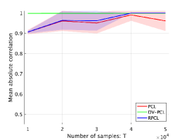
(a) $L=1$

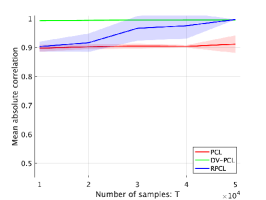
(b) $L=2$

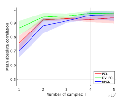
(c) $L=3$

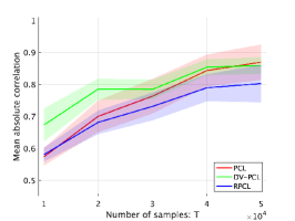
(d) $L=4$

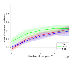
(e) $L=5$

Figure 1: Sample efficiency of nonlinear ICA methods in the case of no outliers (i.e., $\epsilon=0$). The averages of the mean absolute correlation were computed over $10$ runs. $L$ denotes the number of layers both in the nonlinear mixing function $\bm{f}$ in (8) and representation function $\bm{h}_{\mathrm{x}}$.

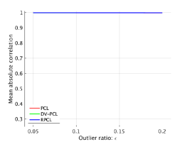
(a) $L=1$

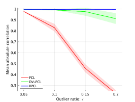
(b) $L=2$

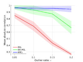
(c) $L=3$

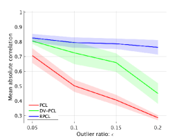
(d) $L=4$

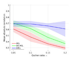
(e) $L=5$

Figure 2: Outlier robustness of nonlinear ICA methods. The averages of the mean absolute correlation were computed over $10$ runs. $L$ denotes the number of layers both in the nonlinear mixing function $\bm{f}$ in (8) and representation function $\bm{h}_{\mathrm{x}}$.

5.1.2 Importance of the dimensionality of complementary data

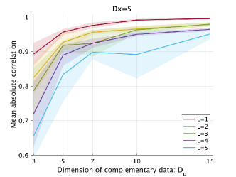
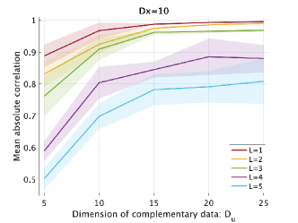
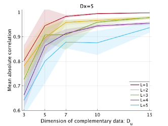
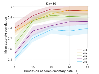
Figure 3: The averages of the mean absolute correlation against the dimensionality of complementary data over $10$ runs. The left and right plots in the first (second) row are $D_{\mathrm{x}}=5$ and $D_{\mathrm{x}}=10$ for Donsker-Varadhan variational estimation ($\gamma$-cross entropy), respectively. $L$ denotes the number of layers both in the nonlinear mixing function $\bm{f}$ in (8) and representation function $\bm{h}_{\mathrm{x}}$.

Next, we investigate how the dimensionality of complementary data $\bm{u}$ affects the source recovery in nonlinear ICA as implied in Proposition 2 and Theorem 3.

We followed the recovery conditions in Theorem 3. In order for the conditional density $p(\bm{s}|\bm{u})$ to be differentiable, the conditionally independent sources were first generated from

$$p(\bm{s}|\bm{u})\propto\prod_{i=1}^{D_{\mathrm{x}}}\exp\left(-\log(\cosh(s_{i}-\bm{w}_{i}^{\mathrm{s}\top}\bm{u}))\right),$$ (43)

where $\bm{w}^{\mathrm{s}}_{i},~{}i=1\dots,D_{\mathrm{x}}$ are $D_{\mathrm{u}}$-dimensional vectors randomly determined from the independent uniform density on $[-1,1]^{D_{\mathrm{u}}}$. The function $\log(\cosh(\cdot))$ is a smooth approximation of the absolute function $|\cdot|$, and thus $p(\bm{s}|\bm{u})$ can be regarded as a smoothed version of the Laplace density (40) in Section 5.1.1. This smooth approximation has been previously used in linear ICA as well (Hyvärinen, 1999). In this experiment, complementary data samples $\bm{u}(t)$ were simply drawn from the independent uniform density on $[0,1]^{D_{\mathrm{u}}}$. The total number of samples is $T=100,000$. Input data $\bm{x}$ was generated according to (8) where the mixing function $\bm{f}$ is modelled by a feedforward neural network with random connections.

Here, we used the nonlinear ICA methods based on the $\gamma$-cross entropy $\widehat{J}_{\mathrm{\gamma}}$ (Section 4.1) and Donsker-Varadhan variational estimation $\widehat{J}_{\mathrm{DV}}$ (Section 4.2). As in Section 5.1.1, the representation function $\bm{h}_{\mathrm{x}}$ was modelled by a feedforward neural network where the number of hidden units was $4D_{\mathrm{x}}$, but the final layer was $D_{\mathrm{x}}$. The number of layers was the same as $\bm{f}$ in the data generative model. $\bm{h}_{\mathrm{u}}(\bm{u})$ was modelled by a one-layer neural network without the activation function as $\bm{h}_{\mathrm{u}}(\bm{u})=\bm{W}_{\mathrm{u}}\bm{u}+\bm{b}_{\mathrm{u}}$ where $\bm{W}_{\mathrm{u}}\in\mathbb{R}^{D_{\mathrm{x}}\times D_{\mathrm{u}}}$ and $\bm{b}_{\mathrm{u}}\in\mathbb{R}^{D_{\mathrm{x}}}$. Since $p(\bm{s}|\bm{u})$ in (43) is a smoother density, $r(\bm{x},\bm{u})$ was also modelled by a smother function than (42) in Section 5.1.1 as follows:

$$r(\bm{x},\bm{u})=\sum_{i=1}^{D_{\mathrm{x}}}\log(\cosh(a_{i,1}h_{\mathrm{x},i}(\bm{x})+a_{i,2}h_{\mathrm{u},i}(\bm{u})+b_{i}))-(\bar{a}_{i}h_{\mathrm{x},i}(\bm{x})+\bar{b}_{i})^{2}+c.$$

All parameters were optimized by Adam for $1,500$ epochs with mini-batch size $256$ and learning rate $0.001$. The $\ell_{2}$ regularization was also applied as done in Section 5.1.1. For the $\gamma$-cross entropy, the value of $\gamma$ was increased from $0.1$ to $3.0$ during minibatch stochastic gradient at every $100$ epoch. The performance was evaluated by the mean absolute correlation as in Section 5.1.1.

The two plots in the first row of Fig.3 are results for Donsker-Varadhan variational estimation, and clearly show that the performance for source recovery depends on the dimensionality of complementary data. When $D_{\mathrm{u}}<D_{\mathrm{x}}$, the mean correlation is small in all layers. However, when $D_{\mathrm{u}}$ is larger than or equal to $D_{\mathrm{x}}$, the mean correlation gets significantly larger. This is consistent with implication of Theorem 3: In order to recover the source components, the dimensionality of complementary data is larger than or equal to input data (i.e., $D_{\mathrm{x}}\leq D_{\mathrm{u}}$ in Assumption (B^′3)), which has not been revealed in previous work of nonlinear ICA. These empirical results clearly support our theoretical implications, and suggest to use fairly high-dimensional complementary data in practice. Similar results were observed for the $\gamma$-cross entropy as well (the second row of Fig.3). Furthermore, especially for Donsker-Varadhan variational estimation, another interesting point is that higher-dimensional complementary data often decreases the variance of the mean absolute correlation, and this implies that higher-dimensional complementary data takes a role of stabilizing estimation as well.

5.2 Evaluation on downstream linear classification

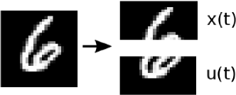
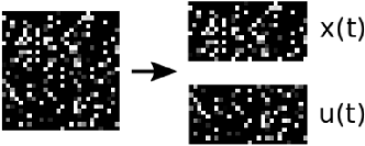
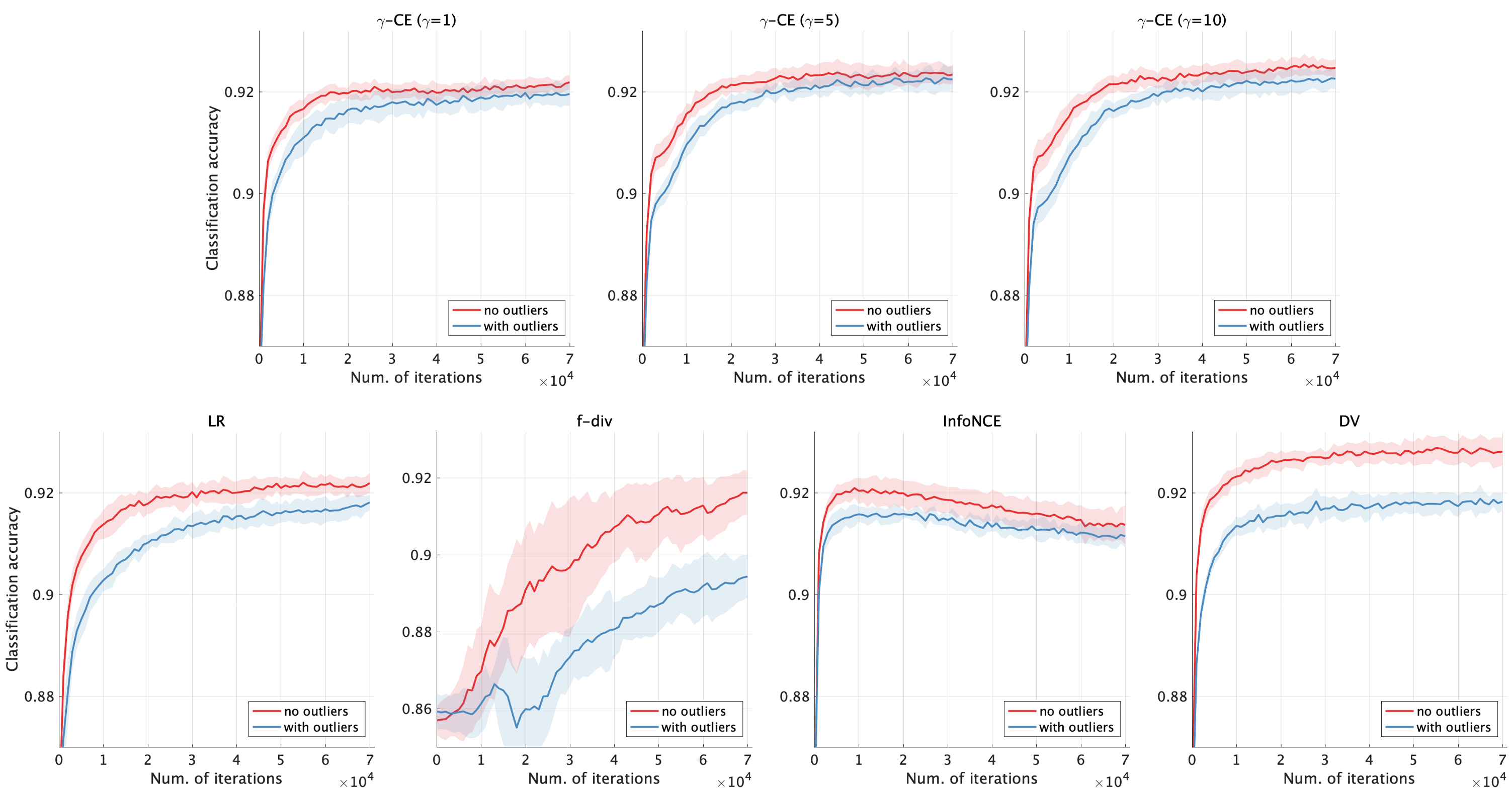
Figure 4: An example of input and complementary data. The half upper images are used for input data samples, while the half below images are complementary ones. The right images are randomly shuffled versions of left images used as outliers.

Figure 5: Averaged classification accuracy for MNIST over $10$ runs. For the red lines, training is performed without outliers, while the blue lines are training with outliers. Note that the scale of the vertical axis only for $f$-div is different.

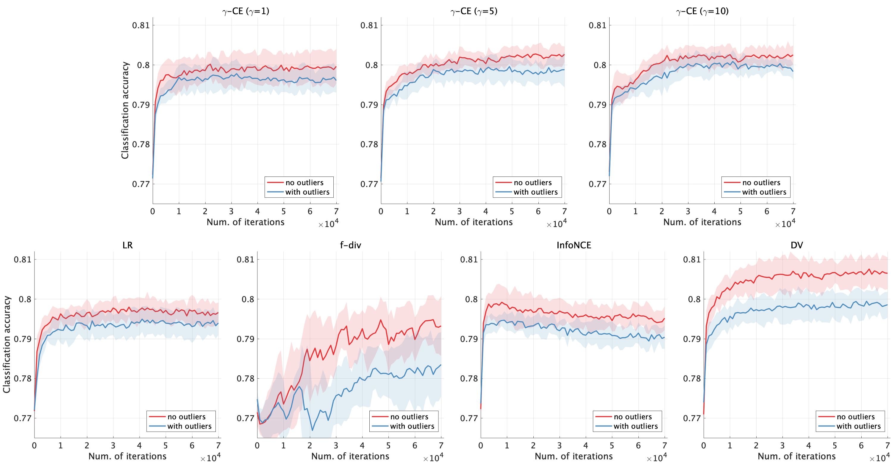
Figure 6: Averaged classification accuracy for Fashion-MNIST over $10$ runs.

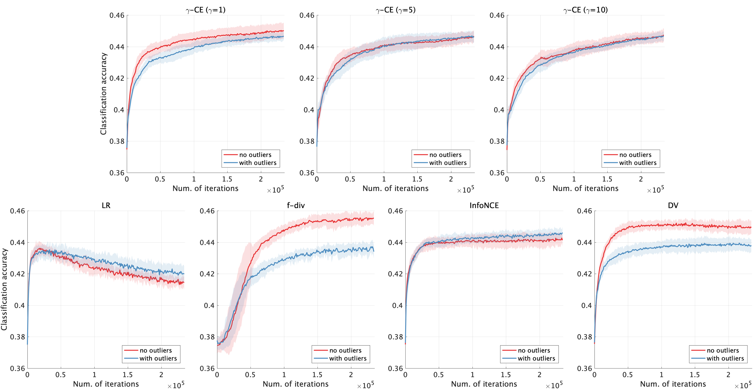
Figure 7: Averaged classification accuracy for CIFAR-10 over $10$ runs.

Table 6: Averages of classification accuracy for the last $5,000$ iterations over $10$ runs. Since we recorded classification accuracy at every $1,000$ iterations, each method includes the $50$ points of the accuracy over $10$ runs. The numbers in parentheses indicate standard deviations. The best and comparable methods judged by the t-test at the significance level 1% are described in boldface.

$\gamma$-CE ($\gamma=5$)	$\gamma$-CE ($\gamma=10$)	LR	f-div.	InfoNCE	DV
MNIST
0.924(0.002)	0.925(0.002)	0.921(0.002)	0.915(0.006)	0.914(0.003)	0.928(0.003)
MNIST with outliers
0.922(0.002)	0.922(0.002)	0.917(0.002)	0.893(0.006)	0.911(0.002)	0.918(0.002)
Fashion-MNIST
0.802(0.003)	0.802(0.003)	0.796(0.003)	0.794(0.006)	0.795(0.003)	0.807(0.004)
Fashion-MNIST with outliers
0.799(0.003)	0.799(0.002)	0.794(0.003)	0.783(0.008)	0.791(0.003)	0.799(0.003)
CIFAR-10
0.446(0.003)	0.447(0.004)	0.414(0.004)	0.455(0.004)	0.442(0.004)	0.449(0.004)
CIFAR-10 with outliers
0.446(0.003)	0.446(0.003)	0.420(0.005)	0.436(0.004)	0.445(0.003)	0.438(0.004)

We finally demonstrate how the proposed method based on the $\gamma$-cross entropy works on benchmark datasets as done in the context of maximization of mutual information (Tschannen et al., 2019), and implicitly investigate Theorem 4 as well because the representation function $\bm{h}_{\mathrm{x}}(\bm{x})$ outputs a lower-dimensional feature than input data. In order to evaluate methods for unsupervised representation learning, a number of protocols have been previously proposed: Multi-scale structural similarity (Wang et al., 2003), mutual information estimation and see more protocols in Hjelm et al. (2019). Here, we employ a linear classification protocol (van den Oord et al., 2018; Tian et al., 2019; Tschannen et al., 2019), which consists of two steps: First, a representation function $\bm{h}_{\mathrm{x}}$ is learned with unlabelled data. Second, the learned representation function is fixed (i.e., not learned anymore), and the feature computed through the representation function is tested on a downstream linear classification task using labelled data. The classification accuracy is the measure for goodness of the representation function.

More specifically, we followed the experimental protocol in Tschannen et al. (2019) , which has been used in the context of deep canonical correlation analysis as well (Andrew et al., 2013). We first divided a single image in half, and then used the upper and lower half images as input $\bm{x}(t)$ and complementary data samples $\bm{u}(t)$, respectively (Left figures in Fig. 5). Based on these data samples $\{\bm{x}(t),\bm{u}(t)\}_{t=1}^{T}$, we applied five methods based on the following objective functions for representation learning:

• $\gamma$-cross entropy ($\gamma$-CE) $\widetilde{J}_{\mathrm{\gamma}}$: In order for initialization, we first updated the parameters in $r(\bm{x},\bm{u})$ with $\gamma=0.1$ for ten epochs, and then used the updated parameters as the initial parameters for the $\gamma$-cross entropy with a larger $\gamma$ value.

• Logistic regression (LR) in (5): LR can be seen as the limit of $\gamma\to{0}$ in the $\gamma$-cross entropy.

• Variational estimation of f-divergence ($f$-div) in (6) (Nguyen et al., 2008; Sugiyama et al., 2008).

• InfoNCE (van den Oord et al., 2018):

  $$\widetilde{J}_{\mathrm{NCE}}(r):=E\left[\frac{1}{K}\sum_{i=1}^{K}\log\frac{e^{r(\bm{x}_{i},\bm{u}_{i})}}{\frac{1}{K}\sum_{j=1}^{K}e^{r(\bm{x}_{i},\bm{u}_{j})}}\right],$$ (44)

  where the expectation is taken over $\prod_{i=1}^{K}p(\bm{x}_{i},\bm{u}_{i})$. In practice, we estimate (44) by averaging over multiple (mini-)batches of samples (Tschannen et al., 2019).

• Donsker-Varadhan variational estimation of mutual information (DV) $\widetilde{J}_{\mathrm{DV}}$ (Ruderman et al., 2012; Belghazi et al., 2018): Unlike nonlinear ICA, this experiment excludes DV from the proposed methods because DV has been already used for maximization of MI (Hjelm et al., 2019).

For all methods, we used the same model $r(\bm{x},\bm{u})$ as

$$r(\bm{x},\bm{u})=\psi(\bm{h}_{\mathrm{x}}(\bm{x}),\bm{h}_{\mathrm{u}}(\bm{u}))+a(\bm{h}_{\mathrm{x}}(\bm{x}))+b(\bm{h}_{\mathrm{u}}(\bm{u})).$$

The representation functions of $\bm{h}_{\mathrm{x}}$ and $\bm{h}_{\mathrm{u}}$ were modelled by the same neural architecture without parameter sharing: The first two hidden layers were convolution layers with the ReLU activation function and the third layer, which is the output layer, was a fully connected layer without the activation function. Before the output layer, we sequentially applied layer normalization (Ba et al., 2016) and average pooling. The output dimensions were fixed at $d_{\mathrm{x}}=d_{\mathrm{u}}=200$. $a(\bm{h}_{\mathrm{x}})$ and $b(\bm{h}_{\mathrm{u}})$ were modelled by a one-layer feedforward network without activation functions. By following van den Oord et al. (2018) and Tian et al. (2019), we set $\psi(\bm{h}_{\mathrm{x}},\bm{h}_{\mathrm{u}})=\bm{h}_{\mathrm{x}}^{\top}\bm{W}\bm{h}_{\mathrm{u}}$ where $\bm{W}$ is a $d_{\mathrm{x}}$ by $d_{\mathrm{u}}$ matrix and learned from data. We optimized all parameters by the Adam optimizer (Kingma and Ba, 2015). After estimating the representation function, $\bm{h}_{\mathrm{x}}(\bm{x})$ was fixed and not learned anymore on the evaluation phase. As evaluation, we only trained a linear classifier to the learned features $\{\bm{h}_{\mathrm{x}}(\bm{x}(t))\}_{t=1}^{T}$ based on multinomial logistic regression. Classification accuracy on test data was used as the evaluation metric.

As datasets, we used the following three classification datasets with ten classes:

• MNIST ($D_{\mathrm{x}}=392,D_{\mathrm{u}}=392$ and $T=60,000$)

• Fashion-MNIST ($D_{\mathrm{x}}=392,D_{\mathrm{u}}=392$ and $T=60,000$)

• CIFAR10 ($D_{\mathrm{x}}=1,536,D_{\mathrm{u}}=1,536$ and $T=50,000$)

For MNIST and Fashion-MNIST, we used the learning rate $10^{-4}$ and updated the parameters for $300$ epochs, while the learning rate for CIFAR10 is $10^{-5}$ and the number of epochs is $1200$. In order to demonstrate the robustness to outliers, the training data was contaminated by randomly shuffled images with respect to pixels (Right figures in Fig. 5). The contamination ratio of outliers was fixed at $0.3$.

Classification accuracy of MNIST on test data samples over iterations is plotted in Fig. 5. In the case of no outliers (i.e., red lines), DV performs the best, while the classification accuracy of the $\gamma$-CE and LR is fairly good. For InfoNCE, the classification accuracy around the $70,000$-th iteration is less than DV, LR and $\gamma$-CE, while $f$-div shows high variance of the classification accuracy over iterations. When data is contaminated by outliers (i.e., blue lines), $f$-div, LR and DV show clear performance degeneration. On the other hand, the performance of $\gamma$-CE is not so influenced by the contamination of outliers. Interestingly, estimation based on InfoNCE is also not strongly hampered by outliers, but the classification accuracy is worse than $\gamma$-CE around the $70000$-th iteration. The same tendency of the robustness of the $\gamma$-cross entropy was observed both for Fashion-MNIST and CIFAR-10 (Figs. 6 and 7). Table 6 quantitatively indicates that the $\gamma$-cross entropy yields the best classification accuracy when data is contaminated by outliers, and shows a fairly good permanence even without outliers. Thus, the proposed method based on the $\gamma$-cross entropy can be robust against outliers as implied in our theoretical analysis and fairly works well even when data is not contaminated by outliers.

Finally, let us note that these results are not trivial because the connection between mutual information and quality of data representation has been experimentally demonstrated to be rather loose (Tian et al., 2019). Thus, it was unclear that robust estimation always leads to robust representations of data. Nonetheless, the proposed method based on the $\gamma$-cross entropy performed the best in the presence of outliers. This means that the proposed robust method for unsupervised representation learning is promising.

6 Conclusion

This paper theoretically showed that density ratio estimation plays a key role in three frameworks for unsupervised representation learning: Maximization of mutual information and nonlinear independent component analysis as well as nonlinear subspace estimation, which is a novel framework proposed in this paper. Furthermore, we made theoretical contributions in each of the three frameworks: We showed that density ratio estimation is necessary and sufficient in maximization of mutual information, while our analysis revealed a novel insight for source recover in nonlinear ICA that the dimensionality of complementary data is an important factor for source recovery, which was clearly supported by numerical experiments. In addition, the proposed generative model in nonlinear subspace estimation is more general than nonlinear ICA in the sense that the latent source components are no longer assumed to be conditionally independent, and theoretical conditions to estimate a nonlinear subspace of the latent source components were given. Motivated by the theoretical results, we developed a nonlinear ICA method by applying an variation lower-bound of mutual information, and proposed an outlier-robust method for unsupervised representation learning through density ratio estimation. We also theoretically investigated their outlier-robustness. The usefulness of the proposed methods were demonstrated through numerical experiments of nonlinear ICA and linear classification in a downstream task.

Acknowledgments

The authors would like to thank Dr. Hiroshi Morioka for sharing his python codes of permutation contrastive learning with us. Takashi Takenouchi was partially supported by JSPS KAKENHI Grant Number 20K03753 and 19H04071.

Appendix A Proof of Theorem 1

Proof  We first recall that $\bm{y}_{\mathrm{x}}:=\bm{h}_{\mathrm{x}}(\bm{x})$ and $\bm{y}_{\mathrm{u}}:=\bm{h}_{\mathrm{u}}(\bm{u})$, and denote $\bm{h}_{\mathrm{x}}^{\perp}(\bm{x})$ and $\bm{h}_{\mathrm{u}}^{\perp}(\bm{u})$ by $\bm{y}_{\mathrm{x}}^{\perp}$ and $\bm{y}_{\mathrm{u}}^{\perp}$, respectively. Based on Assumption (A2), $(\bm{y}_{\mathrm{x}},\bm{y}_{\mathrm{x}}^{\perp}):=(\bm{h}_{\mathrm{x}}(\bm{x}),\bm{h}_{\mathrm{x}}^{\perp}(\bm{x}))$ and $(\bm{y}_{\mathrm{u}},\bm{y}_{\mathrm{u}}^{\perp}):=(\bm{h}_{\mathrm{u}}(\bm{u}),\bm{h}_{\mathrm{u}}^{\perp}(\bm{u}))$ are both invertible in the sense that there exist functions $\bm{g}_{\mathrm{x}}$ and $\bm{g}_{\mathrm{u}}$ such that $\bm{x}=\bm{g}_{\mathrm{x}}(\bm{y}_{\mathrm{x}},\bm{y}_{\mathrm{x}}^{\perp})$ and $\bm{u}=\bm{g}_{\mathrm{u}}(\bm{y}_{\mathrm{u}},\bm{y}_{\mathrm{u}}^{\perp})$. Based on the invertible functions, we first establish the following lemma, which decomposes $I(\mathcal{X},\mathcal{U})$ into three terms:

Lemma 9.

Assumptions (A1-2) hold. Then, $I(\mathcal{X},\mathcal{U})$ can be decomposed as follows:

$$I(\mathcal{X},\mathcal{U}) =I(\mathcal{Y}_{\mathrm{x}},\mathcal{Y}_{\mathrm{u}})+E_{Y_{\mathrm{u}}}[I(\mathcal{Y}_{\mathrm{x}}|\mathcal{Y}_{\mathrm{u}},\mathcal{Y}_{\mathrm{u}}^{\perp}|\mathcal{Y}_{\mathrm{u}})]+E_{\mathrm{Y_{\mathrm{x}}}}[I(\mathcal{Y}_{\mathrm{x}}^{\perp}|\mathcal{Y}_{\mathrm{x}},\mathcal{U}|\mathcal{Y}_{\mathrm{x}})],$$ (45)

where $E_{Y_{\mathrm{u}}}$ and $E_{\mathrm{Y_{\mathrm{x}}}}$ denote the expectations over $p(\bm{y}_{\mathrm{u}})$ and $p(\bm{y}_{\mathrm{x}})$ respectively,

$$I(\mathcal{Y}_{\mathrm{x}}|\mathcal{Y}_{\mathrm{u}},\mathcal{Y}_{\mathrm{u}}^{\perp}|\mathcal{Y}_{\mathrm{u}}) =\iint p(\bm{y}_{\mathrm{x}},\bm{y}_{\mathrm{u}}^{\perp}|\bm{y}_{\mathrm{u}})\log\frac{p(\bm{y}_{\mathrm{x}},\bm{y}_{\mathrm{u}}^{\perp}|\bm{y}_{\mathrm{u}})}{p(\bm{y}_{\mathrm{x}}|\bm{y}_{\mathrm{u}})p(\bm{y}_{\mathrm{u}}^{\perp}|\bm{y}_{\mathrm{u}})}\mathrm{d}\bm{y}_{\mathrm{x}}\mathrm{d}\bm{y}_{\mathrm{u}}^{\perp}$$

$$I(\mathcal{Y}_{\mathrm{x}}^{\perp}|\mathcal{Y}_{\mathrm{x}},\mathcal{U}|\mathcal{Y}_{\mathrm{x}}) :=\iint p(\bm{y}_{\mathrm{x}}^{\perp},\bm{u}|\bm{y}_{\mathrm{x}})\log\frac{p(\bm{y}_{\mathrm{x}}^{\perp},\bm{u}|\bm{y}_{\mathrm{x}})}{p(\bm{y}_{\mathrm{x}}^{\perp}|\bm{y}_{\mathrm{x}})p(\bm{u}|\bm{y}_{\mathrm{x}})}\mathrm{d}\bm{y}_{\mathrm{x}}^{\perp}\mathrm{d}\bm{u}.$$

The proof is given in Appendix A.1. The first term on the right-hand side of (45) is mutual information between the representation functions of $\bm{x}$ and $\bm{u}$, while $I(\mathcal{Y}_{\mathrm{x}}^{\perp}|\mathcal{Y}_{\mathrm{x}},\mathcal{U}|\mathcal{Y}_{\mathrm{x}})$ and $I(\mathcal{Y}_{\mathrm{x}}|\mathcal{Y}_{\mathrm{u}},\mathcal{Y}_{\mathrm{u}}^{\perp}|\mathcal{Y}_{\mathrm{u}})$ measure the conditional independence and are equal to $0$ when $\bm{u}\perp\bm{y}_{\mathrm{x}}^{\perp}|\bm{y}_{\mathrm{x}}$ and $\bm{y}_{\mathrm{x}}\perp\bm{y}_{\mathrm{u}}^{\perp}|\bm{y}_{\mathrm{u}}$. It follows from (45) that $I(\mathcal{X},\mathcal{U})=I(\mathcal{Y}_{\mathrm{x}},\mathcal{Y}_{\mathrm{u}})$ if and only if $I(\mathcal{Y}_{\mathrm{x}}|\mathcal{Y}_{\mathrm{u}},\mathcal{Y}_{\mathrm{u}}^{\perp}|\mathcal{Y}_{\mathrm{u}})=0$ and $I(\mathcal{Y}_{\mathrm{x}}^{\perp}|\mathcal{Y}_{\mathrm{x}},\mathcal{U}|\mathcal{Y}_{\mathrm{x}})=0$.

Next, we fix $\bm{h}_{\mathrm{x}}$ and $\bm{h}_{\mathrm{u}}$ at $\bm{h}_{\mathrm{x}}^{\star}$ and $\bm{h}_{\mathrm{u}}^{\star}$ respectively, and substitute them as $\bm{y}_{\mathrm{x}}=\bm{h}_{\mathrm{x}}^{\star}(\bm{x})$ and $\bm{y}_{\mathrm{u}}=\bm{h}_{\mathrm{u}}^{\star}(\bm{u})$. Then, it is shown that (10) implies both $I(\mathcal{Y}_{\mathrm{x}}|\mathcal{Y}_{\mathrm{u}},\mathcal{Y}_{\mathrm{u}}^{\perp}|\mathcal{Y}_{\mathrm{u}})=0$ and $I(\mathcal{Y}_{\mathrm{x}}^{\perp}|\mathcal{Y}_{\mathrm{x}},\mathcal{U}|\mathcal{Y}_{\mathrm{x}})=0$. We first multiply $p(\bm{u})$ to both sides and rewrite (10) as

$$p(\bm{u}|\bm{x})=p(\bm{u}|\bm{y}_{\mathrm{x}}),$$ (46)

where with the partition function $Z(\bm{y}_{\mathrm{x}}):=\int\exp\left(\psi^{\star}(\bm{y}_{\mathrm{x}},\bm{h}_{\mathrm{u}}^{\star}(\bm{u}))+a^{\star}(\bm{y}_{\mathrm{x}})+b^{\star}(\bm{h}_{\mathrm{u}}^{\star}(\bm{u}))\right)p(\bm{u})\mathrm{d}\bm{u}$,

$$p(\bm{u}|\bm{y}_{\mathrm{x}}):=\frac{\exp\left(\psi^{\star}(\bm{y}_{\mathrm{x}},\bm{h}_{\mathrm{u}}^{\star}(\bm{u})))+a^{\star}(\bm{y}_{\mathrm{x}})+b^{\star}(\bm{h}_{\mathrm{u}}^{\star}(\bm{u}))\right)p(\bm{u})}{Z(\bm{y}_{\mathrm{x}})}.$$

By the invertible assumption for $(\bm{y}_{\mathrm{x}},\bm{y}_{\mathrm{x}}^{\perp})$, (46) can be equivalently expressed as the following conditional independence:

$$\bm{u}\perp\bm{y}_{\mathrm{x}}^{\perp}|\bm{y}_{\mathrm{x}},$$ (47)

implying that

$$I(\mathcal{Y}_{\mathrm{x}}^{\perp}|\mathcal{Y}_{\mathrm{x}},\mathcal{U}|\mathcal{Y}_{\mathrm{x}})=0.$$

Similarly, we can derive the following equation from (10):

$$p(\bm{x}|\bm{u})=p(\bm{x}|\bm{y}_{\mathrm{u}}),$$ (48)

where with the partition function $Z(\bm{y}_{\mathrm{u}}):=\int\exp\left(\psi^{\star}(\bm{h}_{\mathrm{x}}^{\star}(\bm{x}),\bm{y}_{\mathrm{u}})+a^{\star}(\bm{h}_{\mathrm{x}}^{\star}(\bm{x}))+b^{\star}(\bm{y}_{\mathrm{u}})\right)p(\bm{x})\mathrm{d}\bm{x}$,

$$p(\bm{x}|\bm{y}_{\mathrm{u}}):=\frac{\exp\left(\psi^{\star}(\bm{h}_{\mathrm{x}}^{\star}(\bm{x}),\bm{y}_{\mathrm{u}})+a^{\star}(\bm{h}_{\mathrm{x}}^{\star}(\bm{x}))+b^{\star}(\bm{y}_{\mathrm{u}})\right)p(\bm{x})}{Z(\bm{y}_{\mathrm{u}})}.$$

Again, (48) implies the conditional independence as

$$\bm{x}\perp\bm{y}_{\mathrm{u}}^{\perp}|\bm{y}_{\mathrm{u}}.$$ (49)

Data processing inequality and conditional independence (49) lead to

$$I(\mathcal{Y}_{\mathrm{x}}|\mathcal{Y}_{\mathrm{u}},\mathcal{Y}_{\mathrm{u}}^{\perp}|\mathcal{Y}_{\mathrm{u}})\leq{I}(\mathcal{X}|\mathcal{Y}_{\mathrm{u}},\mathcal{Y}_{\mathrm{u}}^{\perp}|\mathcal{Y}_{\mathrm{u}})\underset{\eqref{cond-ind-hy}}{=}0.$$

Both $I(\mathcal{Y}_{\mathrm{x}}|\mathcal{Y}_{\mathrm{u}},\mathcal{Y}_{\mathrm{u}}^{\perp}|\mathcal{Y}_{\mathrm{u}})=0$ and $I(\mathcal{Y}_{\mathrm{x}}^{\perp}|\mathcal{Y}_{\mathrm{x}},\mathcal{U}|\mathcal{Y}_{\mathrm{x}})=0$ enable us to ensure $I(\mathcal{X},\mathcal{U})=I(\mathcal{Y}_{\mathrm{x}},\mathcal{Y}_{\mathrm{u}})$.

Conversely, we suppose that $I(\mathcal{X},\mathcal{U})=I(\mathcal{Y}_{\mathrm{x}},\mathcal{Y}_{\mathrm{u}})$ at $\bm{h}_{\mathrm{x}}=\bm{h}_{\mathrm{x}}^{\star}$ and $\bm{h}_{\mathrm{u}}=\bm{h}_{\mathrm{u}}^{\star}$. Then, it follows from (45) that $I(\mathcal{Y}_{\mathrm{x}}|\mathcal{Y}_{\mathrm{u}},\mathcal{Y}_{\mathrm{u}}^{\perp}|\mathcal{Y}_{\mathrm{u}})=0$ and $I(\mathcal{Y}_{\mathrm{x}}^{\perp}|\mathcal{Y}_{\mathrm{x}},\mathcal{U}|\mathcal{Y}_{\mathrm{x}})=0$. $I(\mathcal{Y}_{\mathrm{x}}^{\perp}|\mathcal{Y}_{\mathrm{x}},\mathcal{U}|\mathcal{Y}_{\mathrm{x}})=0$ means the conditional independence (47), which can be equivalently expressed as (46). On the other hand, under the invertibility of $(\bm{y}_{\mathrm{u}},\bm{y}_{\mathrm{u}}^{\perp})$, $I(\mathcal{Y}_{\mathrm{x}}|\mathcal{Y}_{\mathrm{u}},\mathcal{Y}_{\mathrm{u}}^{\perp}|\mathcal{Y}_{\mathrm{u}})=0$ implies

$$\bm{y}_{\mathrm{x}}\perp\bm{y}_{\mathrm{u}}^{\perp}|\bm{y}_{\mathrm{u}}\quad\text{or equivalently}\quad p(\bm{y}_{\mathrm{x}}|\bm{u})=p(\bm{y}_{\mathrm{x}}|\bm{y}_{\mathrm{u}}).$$ (50)

A simple calculation yields

$$p(\bm{x},\bm{u}) =p(\bm{u}|\bm{x})p(\bm{x})\underset{\eqref{SDRcond}}{=}p(\bm{u}|\bm{y}_{\mathrm{x}})p(\bm{x})\underset{(\star)}{=}\frac{p(\bm{y}_{\mathrm{x}}|\bm{u})p(\bm{u})}{p(\bm{y}_{\mathrm{x}})}p(\bm{x})\underset{\eqref{SDRcond3}}{=}\frac{p(\bm{y}_{\mathrm{x}}|\bm{y}_{\mathrm{u}})}{p(\bm{y}_{\mathrm{x}})}p(\bm{x})p(\bm{u}),$$ (51)

where we applied Bayes’ theorem on $(\star)$. By dividing both sides of (51) by $p(\bm{x})p(\bm{u})$, we have

$$\log\frac{p(\bm{x},\bm{u})}{p(\bm{x})p(\bm{u})}=\log{p}(\bm{y}_{\mathrm{x}},\bm{y}_{\mathrm{u}})-\log{p}(\bm{y}_{\mathrm{x}})-\log{p}(\bm{y}_{\mathrm{u}}).$$

The existence of the functions is obvious by denoting $\log p(\bm{y}_{\mathrm{x}},\bm{y}_{\mathrm{u}})$, $-\log{p}(\bm{y}_{\mathrm{x}})$ and $-\log{p}(\bm{y}_{\mathrm{u}})$ by $\psi^{\star}(\bm{y}_{\mathrm{x}},\bm{y}_{\mathrm{u}})$, $a^{\star}(\bm{y}_{\mathrm{x}})$ and $b^{\star}(\bm{y}_{\mathrm{u}})$ respectively. The proof is completed.  

A.1 Proof of Lemma 9

Proof  We first decompose $I(\mathcal{X},\mathcal{U})$ based on the invertibility assumption of $(\bm{y}_{\mathrm{x}},\bm{y}_{\mathrm{x}}^{\perp})$ as follows:

$$I(\mathcal{X},\mathcal{U}) =\iiint p(\bm{y}_{\mathrm{x}},\bm{y}_{\mathrm{x}}^{\perp},\bm{u})\log\frac{p(\bm{y}_{\mathrm{x}},\bm{y}_{\mathrm{x}}^{\perp},\bm{u})}{p(\bm{y}_{\mathrm{x}},\bm{y}_{\mathrm{x}}^{\perp})p(\bm{u})}\mathrm{d}\bm{y}_{\mathrm{x}}\mathrm{d}\bm{y}_{\mathrm{x}}^{\perp}\mathrm{d}\bm{u}$$

$$=\iint p(\bm{y}_{\mathrm{x}},\bm{u})\log\frac{p(\bm{y}_{\mathrm{x}},\bm{u})}{p(\bm{y}_{\mathrm{x}})p(\bm{u})}\mathrm{d}\bm{y}_{\mathrm{x}}\mathrm{d}\bm{u}$$

$$\qquad+\int{p}(\bm{y}_{\mathrm{x}})\left[\iint p(\bm{y}_{\mathrm{x}}^{\perp},\bm{u}|\bm{y}_{\mathrm{x}})\log\frac{p(\bm{y}_{\mathrm{x}}^{\perp},\bm{u}|\bm{y}_{\mathrm{x}})}{p(\bm{y}_{\mathrm{x}}^{\perp}|\bm{y}_{\mathrm{x}})p(\bm{u}|\bm{y}_{\mathrm{x}})}\mathrm{d}\bm{u}\mathrm{d}\bm{y}_{\mathrm{x}}^{\perp}\right]\mathrm{d}\bm{y}_{\mathrm{x}}$$

$$=I(\mathcal{Y}_{\mathrm{x}},\mathcal{U})+E_{\mathrm{Y}_{\mathrm{x}}}[I(\mathcal{Y}_{\mathrm{x}}^{\perp}|\mathcal{Y}_{\mathrm{x}},\mathcal{U}|\mathcal{Y}_{\mathrm{x}})],$$ (52)

where we used the following relation:

$$\frac{p(\bm{y}_{\mathrm{x}},\bm{y}_{\mathrm{x}}^{\perp},\bm{u})}{p(\bm{y}_{\mathrm{x}},\bm{y}_{\mathrm{x}}^{\perp})p(\bm{u})} =\frac{p(\bm{y}_{\mathrm{x}}^{\perp},\bm{u}|\bm{y}_{\mathrm{x}})p(\bm{y}_{\mathrm{x}})}{p(\bm{y}_{\mathrm{x}}^{\perp}|\bm{y}_{\mathrm{x}})p(\bm{y}_{\mathrm{x}})p(\bm{u})}\cdot\frac{p(\bm{y}_{\mathrm{x}},\bm{u})}{p(\bm{y}_{\mathrm{x}},\bm{u})}=\frac{p(\bm{y}_{\mathrm{x}},\bm{u})}{p(\bm{y}_{\mathrm{x}})p(\bm{u})}\cdot\frac{p(\bm{y}_{\mathrm{x}}^{\perp},\bm{u}|\bm{y}_{\mathrm{x}})}{p(\bm{y}_{\mathrm{x}}^{\perp}|\bm{y}_{\mathrm{x}})p(\bm{u}|\bm{y}_{\mathrm{x}})}.$$

Applying the same decomposition as (52) to $I(\mathcal{Y}_{\mathrm{x}},\mathcal{U})$ under the change of variables by the invertible $(\bm{y}_{\mathrm{u}},\bm{y}_{\mathrm{u}}^{\perp})$ yields

$$I(\mathcal{Y}_{\mathrm{x}},\mathcal{U}) =\iiint{p}(\bm{y}_{\mathrm{x}},\bm{y}_{\mathrm{u}},\bm{y}_{\mathrm{u}}^{\perp})\log\frac{p(\bm{y}_{\mathrm{x}},\bm{y}_{\mathrm{u}},\bm{y}_{\mathrm{u}}^{\perp})}{p(\bm{y}_{\mathrm{x}})p(\bm{y}_{\mathrm{u}},\bm{y}_{\mathrm{u}}^{\perp})}\mathrm{d}\bm{y}_{\mathrm{x}}\mathrm{d}\bm{y}_{\mathrm{u}}\mathrm{d}\bm{y}_{\mathrm{u}}^{\perp}$$

$$=\iint{p}(\bm{y}_{\mathrm{x}},\bm{y}_{\mathrm{u}})\log\frac{p(\bm{y}_{\mathrm{x}},\bm{y}_{\mathrm{u}})}{p(\bm{y}_{\mathrm{x}})p(\bm{y}_{\mathrm{u}})}\mathrm{d}\bm{y}_{\mathrm{x}}\mathrm{d}\bm{y}_{\mathrm{u}}$$

$$\qquad+\int{p}(\bm{y}_{\mathrm{u}})\left[\iint p(\bm{y}_{\mathrm{x}},\bm{y}_{\mathrm{u}}^{\perp}|\bm{y}_{\mathrm{u}})\log\frac{p(\bm{y}_{\mathrm{x}},\bm{y}_{\mathrm{u}}^{\perp}|\bm{y}_{\mathrm{u}})}{p(\bm{y}_{\mathrm{u}}^{\perp}|\bm{y}_{\mathrm{u}})p(\bm{y}_{\mathrm{x}}|\bm{y}_{\mathrm{u}})}\mathrm{d}\bm{y}_{\mathrm{x}}\mathrm{d}\bm{y}_{\mathrm{u}}^{\perp}\right]\mathrm{d}\bm{y}_{\mathrm{u}}$$

$$=I(\mathcal{Y}_{\mathrm{x}},\mathcal{Y}_{\mathrm{u}})+E_{\mathrm{Y}_{\mathrm{u}}}[I(\mathcal{Y}_{\mathrm{x}}|\mathcal{Y}_{\mathrm{u}},\mathcal{Y}_{\mathrm{u}}^{\perp}|\mathcal{Y}_{\mathrm{u}})],$$ (53)

where we used

$$\frac{p(\bm{y}_{\mathrm{x}},\bm{y}_{\mathrm{u}},\bm{y}_{\mathrm{u}}^{\perp})}{p(\bm{y}_{\mathrm{x}})p(\bm{y}_{\mathrm{u}},\bm{y}_{\mathrm{u}}^{\perp})}=\frac{p(\bm{y}_{\mathrm{x}},\bm{y}_{\mathrm{u}}^{\perp}|\bm{y}_{\mathrm{u}})p(\bm{y}_{\mathrm{u}})}{p(\bm{y}_{\mathrm{x}})p(\bm{y}_{\mathrm{u}}^{\perp}|\bm{y}_{\mathrm{u}})p(\bm{y}_{\mathrm{u}})}\cdot\frac{p(\bm{y}_{\mathrm{x}},\bm{y}_{\mathrm{u}})}{p(\bm{y}_{\mathrm{x}},\bm{y}_{\mathrm{u}})}=\frac{p(\bm{y}_{\mathrm{x}},\bm{y}_{\mathrm{u}})}{p(\bm{y}_{\mathrm{x}})p(\bm{y}_{\mathrm{u}})}\cdot\frac{p(\bm{y}_{\mathrm{x}},\bm{y}_{\mathrm{u}}^{\perp}|\bm{y}_{\mathrm{u}})}{p(\bm{y}_{\mathrm{u}}^{\perp}|\bm{y}_{\mathrm{u}})p(\bm{y}_{\mathrm{x}}|\bm{y}_{\mathrm{u}})}$$

Substituting (53) into (52) completes the proof.  

Appendix B Proof of Proposition 2

Proof  Let us denote the inverse of the mixing function $\bm{f}$ in the generative model (8) as $\bm{g}:=\bm{f}^{-1}$. From the conditional independence of $\bm{s}$ given $\bm{u}$ in Assumption (B1), we obtain the conditional density of $\bm{x}$ given $\bm{u}$ under the change of variables by $\bm{s}=\bm{g}(\bm{x})$ as follows:

$$\log p(\bm{x}|\bm{u}) =\sum_{i=1}^{D_{\mathrm{x}}}q_{i}(g_{i}(\bm{x}),\bm{u})+\log|\det\bm{J}_{\bm{g}}(\bm{x})|-\log{Z}(\bm{u}),$$ (54)

where $\bm{g}(\bm{x})=(g_{1}(\bm{x}),g_{2}(\bm{x}),\dots,g_{D_{\mathrm{x}}}(\bm{x}))^{\top}$ and $\bm{J}_{\bm{g}}(\bm{x})$ is the Jacobian of $\bm{g}$ at $\bm{x}$. Similarly, by applying the same change of variables for the marginal density of $\bm{s}$, the marginal density of $\bm{x}$ is given by

$$\log{p}(\bm{x}) =\log{p}(\bm{g}(\bm{x}))+\log|\det\bm{J}_{\bm{g}}(\bm{x})|.$$ (55)

On the other hand, the log-density ratio equation (11) yields

$$\log p(\bm{x}|\bm{u})-\log p(\bm{x})=\sum_{i=1}^{D_{\mathrm{x}}}\psi^{\star}_{i}(h_{\mathrm{x},i}^{\star}(\bm{x}),\bm{h}_{\mathrm{u}}^{\star}(\bm{u}))+a^{\star}(\bm{h}_{\mathrm{x}}^{\star}(\bm{x}))+b^{\star}(\bm{h}_{\mathrm{u}}^{\star}(\bm{u})).$$ (56)

Substitution of (54) and (55) into the left-hand side of (56) cancels out the Jacobian term and gives the following equation:

$$\sum_{i=1}^{D_{\mathrm{x}}}q_{i}(g_{i}(\bm{x}),\bm{u})-\log{Z}(\bm{u})-\log p(\bm{g}(\bm{x}))=\sum_{i=1}^{D_{\mathrm{x}}}\psi_{i}^{\star}(h_{\mathrm{x},i}^{\star}(\bm{x}),\bm{h}_{\mathrm{u}}^{\star}(\bm{u}))+a^{\star}(\bm{h}_{\mathrm{x}}^{\star}(\bm{x}))+b^{\star}(\bm{h}_{\mathrm{u}}^{\star}(\bm{u})).$$ (57)

Then, we compute the gradient of the both sides on (57) with respect to $\bm{u}$ as

$$\sum_{i=1}^{D_{\mathrm{x}}}\nabla_{\bm{u}}q_{i}(g_{i}(\bm{x}),\bm{u})-\nabla_{\bm{u}}\log{Z}(\bm{u})=\sum_{i=1}^{D_{\mathrm{x}}}\nabla_{\bm{u}}\psi_{i}^{\star}(h_{\mathrm{x},i}^{\star}(\bm{x}),\bm{h}_{\mathrm{u}}^{\star}(\bm{u}))+\nabla_{\bm{u}}b^{\star}(\bm{h}_{\mathrm{u}}^{\star}(\bm{u})).$$

By using the notations of $\bm{z}:=\bm{h}_{\mathrm{x}}^{\star}(\bm{x})$ and $\bm{v}(\bm{z}):=\bm{g}((\bm{h}_{\mathrm{x}}^{\star})^{-1}(\bm{z}))$ where $(\bm{h}_{\mathrm{x}}^{\star})^{-1}$ denotes the inverse of $\bm{h}_{\mathrm{x}}^{\star}$,

$$\sum_{i=1}^{D_{\mathrm{x}}}\nabla_{\bm{u}}q_{i}(v_{i}(\bm{z}),\bm{u})-\nabla_{\bm{u}}\log{Z}(\bm{u})=\sum_{i=1}^{D_{\mathrm{x}}}\nabla_{\bm{u}}\psi_{i}^{\star}(z_{i},\bm{h}_{\mathrm{u}}^{\star}(\bm{u}))+\nabla_{\bm{u}}b^{\star}(\bm{h}_{\mathrm{u}}^{\star}(\bm{u})),$$ (58)

where $z_{i}$ and $v_{i}$ are the $i$-th elements in $\bm{z}$ and $\bm{v}$, respectively.

Next, we show from (58) that each element in $\bm{v}(\bm{z})(=\bm{s})$ is a function of a distinct and single element in $\bm{z}(=\bm{h}_{\mathrm{x}}^{\star}(\bm{x}))$. To this end, we first take the partial derivative to both sides on (58) with respect to $z_{l}$ as

$$\sum_{i=1}^{D_{\mathrm{x}}}v_{i}^{(l)}(\bm{z})\nabla_{\bm{u}}q_{i}^{\prime}(v_{i}(\bm{z}),\bm{u})=\frac{\partial}{\partial z_{l}}\left[\nabla_{\bm{u}}\psi_{l}^{\star}(z_{l},\bm{h}_{\mathrm{u}}^{\star}(\bm{u}))\right],$$ (59)

where $q_{i}^{\prime}(t,\bm{u}):=\frac{\partial q_{i}(t,\bm{u})}{\partial t}$ and $v_{i}^{(l)}(\bm{z}):=\frac{\partial v_{i}(\bm{z})}{\partial z_{l}}$. We further take the partial derivative of both sides on (59) with respect to $z_{m}$ for $m\neq l$ as

$$\sum_{i=1}^{D_{\mathrm{x}}}\left[v_{i}^{(l,m)}(\bm{z})\nabla_{\bm{u}}q_{i}^{\prime}(v_{i}(\bm{z}),\bm{u})+v_{i}^{(l)}(\bm{z})v_{i}^{(m)}(\bm{z})\nabla_{\bm{u}}q_{i}^{\prime\prime}(v_{i}(\bm{z}),\bm{u})\right]=\bm{0},$$ (60)

where $q_{i}^{\prime\prime}(t,\bm{u}):=\frac{\partial^{2}}{\partial t^{2}}q_{i}(t,\bm{u})$ and $v_{i}^{(l,m)}(\bm{z}):=\frac{\partial^{2}}{\partial z_{l}\partial z_{m}}v_{i}(\bm{z})$. In order to express (60) as a matrix form, we define the $D_{\mathrm{x}}(D_{\mathrm{x}}-1)/2$ by $2D_{\mathrm{x}}$ matrix consisting of a collection of $v_{i}^{(l)}(\bm{z})v_{i}^{(m)}(\bm{z})$ and $v_{i}^{(l,m)}(\bm{z})$ with respect to $i,l,m$ ($l\neq{m}$) as

$$\bm{M}(\bm{v}) :=\left(\begin{array}[]{cccccc}v_{1}^{(1,2)}&\cdots&v_{D_{\mathrm{x}}}^{(1,2)}&v_{1}^{(1)}v_{1}^{(2)}&\cdots&v_{D_{\mathrm{x}}}^{(1)}v_{D_{\mathrm{x}}}^{(2)}\\ v_{1}^{(1,3)}&\cdots&v_{D_{\mathrm{x}}}^{(1,3)}&v_{1}^{(1)}v_{1}^{(3)}&\cdots&v_{D_{\mathrm{x}}}^{(1)}v_{D_{\mathrm{x}}}^{(3)}\\ \vdots&\vdots&\vdots&\cdots&\vdots&\vdots\\ v_{1}^{(D_{\mathrm{x}}-1,D_{\mathrm{x}})}&\cdots&v_{D_{\mathrm{x}}}^{(D_{\mathrm{x}}-1,D_{\mathrm{x}})}&v_{1}^{(D_{\mathrm{x}}-1)}v_{1}^{(D_{\mathrm{x}})}&\cdots&v_{D_{\mathrm{x}}}^{(D_{\mathrm{x}}-1)}v_{D_{\mathrm{x}}}^{(D_{\mathrm{x}})}\\ \end{array}\right)\in\mathbb{R}^{\frac{D_{\mathrm{x}}(D_{\mathrm{x}}-1)}{2}\times{2}D_{\mathrm{x}}}.$$

We also define a collection of $q^{\prime}_{i}(v_{i}(\bm{z}),\bm{u})$ and $q^{\prime\prime}_{i}(v_{i}(\bm{z}),\bm{u})$ by the following $2D_{\mathrm{x}}$-dimensional vector:

$$\bm{w}(\bm{v},\bm{u}) :=\left(q^{\prime}_{1}(v_{1},\bm{u}),\dots,q^{\prime}_{D_{\mathrm{x}}}(v_{D_{\mathrm{x}}},\bm{u}),q^{\prime\prime}_{1}(v_{1},\bm{u}),\dots,q^{\prime\prime}_{D_{\mathrm{x}}}(v_{D_{\mathrm{x}}},\bm{u})\right)^{\top}\in\mathbb{R}^{{2}D_{\mathrm{x}}}.$$

By fixing $\bm{u}$ at $\bm{u}=\bm{u}_{1}$, (60) can be expressed by using $\bm{M}(\bm{v})$ and $\bm{w}(\bm{v},\bm{u})$ as

$$\bm{M}(\bm{v})\bm{W}(\bm{v})=\bm{O},$$ (61)

where $\bm{W}(\bm{v}):=\nabla_{\bm{u}}\bm{w}(\bm{v},\bm{u})\Bigr{|}_{\bm{u}=\bm{u}_{1}}\in\mathbb{R}^{2D_{\mathrm{x}}\times D_{\mathrm{u}}}$ and $\bm{O}$ denotes the null matrix. Since Assumptions (B3-4) ensure that the rank of $\bm{W}(\bm{v})$ is $2D_{\mathrm{x}}$, $\bm{W}(\bm{v})\bm{W}(\bm{v})^{\top}$ is a $2D_{\mathrm{x}}$ by $2D_{\mathrm{x}}$ invertible matrix. Thus, multiplying $\bm{W}(\bm{v})^{\top}$ to (61) and taking the inverse of $\bm{W}(\bm{v})\bm{W}(\bm{v})^{\top}$ on the right yields

$$\bm{M}(\bm{v})=\bm{O}.$$ (62)

Eq.(62) indicates that $v_{i}^{(l,m)}(\bm{z})=0$ and $v_{i}^{(l)}(\bm{z})v_{i}^{(m)}(\bm{z})=0$ for all $i,l,m=1,\dots,D_{\mathrm{x}}$ with $l\neq{m}$. This means that each element in $\bm{v}(\bm{z})$ is a function of a distinct and single element in $\bm{z}$ because $\bm{v}(\bm{z})$ is an invertible function. Thus, the proof is completed.  

Appendix C Rank condition in the exponential family

We first express the exponential family (12) as

$$\log{p}(\bm{s}|\bm{u})=\sum_{k=1}^{K}\bm{\lambda}_{k}(\bm{u})^{\top}\bm{q}_{k}(\bm{s})-\log{Z}(\bm{u}),$$

where $\bm{\lambda}_{k}(\bm{u}):=(\lambda_{1k}(\bm{u}),\dots,\lambda_{D_{\mathrm{x}}{k}}(\bm{u}))^{\top}$ and $\bm{q}_{k}(\bm{s}):=(q_{1k}(s_{1}),\dots,q_{D_{\mathrm{x}}{k}}(s_{D_{\mathrm{x}}}))$. Then, a simple computation yields

$$\nabla_{\bm{u}}\bm{w}(\bm{v},\bm{u})=\sum_{k=1}^{K}\bm{\Lambda}_{k}\odot\bm{Q}_{k},$$ (63)

where $\odot$ denotes the Hadamard product (i.e., elementwise multiplication of two matrices)

$$\bm{\Lambda}_{k}:=\left(\begin{array}[]{c}\nabla_{\bm{u}}\bm{\lambda}_{k}(\bm{u})\\ \nabla_{\bm{u}}\bm{\lambda}_{k}(\bm{u})\end{array}\right),$$

and with $q^{\prime}_{ik}(t):=\frac{\mathrm{d}}{\mathrm{d}{t}}q_{ik}(t)$ and $q^{\prime\prime}_{ik}(t):=\frac{\mathrm{d}^{2}}{\mathrm{d}{t}^{2}}q_{ik}(t)$ for $i=1,\dots,D_{\mathrm{x}}$,

$${\bm{Q}}_{k}=\left(\begin{array}[]{cccc}q^{\prime}_{1k}(v_{1})&q^{\prime}_{1k}(v_{1})&\cdots&q^{\prime}_{1k}(v_{1})\\ \vdots&\vdots&\cdots&\vdots\\ q^{\prime}_{D_{\mathrm{x}}{k}}(v_{D_{\mathrm{x}}})&q^{\prime}_{D_{\mathrm{x}}{k}}(v_{D_{\mathrm{x}}})&\cdots&q^{\prime}_{D_{\mathrm{x}}{k}}(v_{D_{\mathrm{x}}})\\ q^{\prime\prime}_{1k}(v_{1})&q^{\prime\prime}_{1k}(v_{1})&\cdots&q^{\prime\prime}_{1k}(v_{1})\\ \vdots&\vdots&\cdots&\vdots\\ q^{\prime\prime}_{D_{\mathrm{x}}{k}}(v_{D_{\mathrm{x}}})&q^{\prime\prime}_{D_{\mathrm{x}}{k}}(v_{D_{\mathrm{x}}})&\cdots&q^{\prime\prime}_{D_{\mathrm{x}}{k}}(v_{D_{\mathrm{x}}})\end{array}\right).$$

The rank of $\bm{\Lambda}_{k}$ is at most $D_{\mathrm{x}}$ under Assumption (B3) because $\bm{\Lambda}_{k}$ is a vertical concatenation of the two same matrices of $\nabla_{\bm{u}}\bm{\lambda}_{k}(\bm{u})\in\mathbb{R}^{D_{\mathrm{x}}\times D_{\mathrm{u}}}$. On the other hand, $\bm{Q}_{k}$ is a rank-one matrix because the column vectors in ${\bm{Q}}_{k}$ are all same. Thus, the rank factorization ensures that the following decompositions of $\bm{\Lambda}_{k}$ and $\bm{Q}_{k}$ exist:

$$\bm{\Lambda}_{k}=\sum_{i=1}^{D_{\mathrm{x}}}\bm{a}_{ik}\bm{b}_{ik}^{\top}\quad~{}\text{and}\quad~{}{\bm{Q}}_{k}=\bm{c}_{k}\bm{d}_{k}^{\top},$$ (64)

where $\bm{a}_{ik},\bm{c}_{k}\in\mathbb{R}^{2D_{\mathrm{x}}}$ and $\bm{b}_{ik},\bm{d}_{k}\in\mathbb{R}^{D_{\mathrm{u}}}$. Substituting (64) into (63) yields

$$\nabla_{\bm{u}}\bm{w}(\bm{v},\bm{u})=\sum_{k=1}^{K}\sum_{i=1}^{D_{\mathrm{x}}}(\bm{a}_{ik}\odot\bm{c}_{k})(\bm{b}_{ik}\odot\bm{d}_{k})^{\top}.$$ (65)

indicating that the rank of $\nabla_{\bm{u}}\bm{w}(\bm{v},\bm{u})$ is at most $2D_{\mathrm{x}}$ when $K>1$. On the other hand, when $K=1$, (65) is given by

$$\nabla_{\bm{u}}\bm{w}(\bm{v},\bm{u})=\sum_{i=1}^{D_{\mathrm{x}}}(\bm{a}_{i1}\odot\bm{c}_{1})(\bm{b}_{i1}\odot\bm{d}_{1})^{\top},$$

and thus the rank is at most $D_{\mathrm{x}}$.

Appendix D Proof of Theorem 3

Our proof is based on the following lemmas:

Lemma 10.

Suppose that $\bm{D}(\bm{v})$ is an $n$ by $n$ diagonal matrix whose diagonals $d_{i}(\bm{v})$ is a function of $\bm{v}\in\mathbb{R}^{n}$, and $\bm{A}$ and $\bm{B}$ are $n$ by $n$ constant matrices. Furthermore, the following assumptions are made:

1. There exist $n$ points $\bm{v}_{1},\bm{v}_{2},\dots,\bm{v}_{n}$ such that $\bm{d}(\bm{v}_{1}),\bm{d}(\bm{v}_{2}),\dots,\bm{d}(\bm{v}_{n})$ are linearly independent where $\bm{d}(\bm{v}):=(d_{1}(\bm{v}),d_{2}(\bm{v}),\dots,d_{n}(\bm{v}))^{\top}$ is the vector of the diagonal elements in $\bm{D}(\bm{v})$.

2. $\bm{A}$ and $\bm{B}$ are of full-rank.

Then, when $\bm{A}\bm{D}(\bm{v})\bm{B}$ is a diagonal matrix at least at $n$ points $\bm{v}_{1},\bm{v}_{2},\dots,\bm{v}_{n}$, then both $\bm{A}$ and $\bm{B}$ are diagonal matrices multiplied by a permutation matrix.

Lemma 11 (Theorem 4.4.8 in Harville (2006)).

Suppose that $\bm{A}$ is an $m$ by $n$ matrix of rank $r$. For any $m$ by $r$ matrix $\bm{B}$ and $r$ by $n$ matrix $\bm{T}$ such that $\bm{A}=\bm{B}\bm{T}$, both $\bm{B}$ and $\bm{T}$ have rank $r$.

Lemma 10 is proved in Appendix D.2, while the reader may refer to the proof of Theorem 4.4.8 in Harville (2006) for Lemma 11.

D.1 Main proof

Proof  We start by using the same notations and following the same line of the proof until (57) in Section B. Then, we obtain the following equation under Assumptions (B^′1-2,6):

$$\sum_{i=1}^{D_{\mathrm{x}}}q_{i}(g_{i}(\bm{x}),\lambda_{i}(\bm{u}))-\log{Z}(\bm{u})-\log p(\bm{g}(\bm{x}))$$

$$\qquad=\sum_{i=1}^{D_{\mathrm{x}}}\psi_{i}^{\star}(h_{\mathrm{x},i}^{\star}(\bm{x}),h_{\mathrm{u},i}^{\star}(\bm{u}))+a^{\star}(\bm{h}_{\mathrm{x}}^{\star}(\bm{x}))+b^{\star}(\bm{h}_{\mathrm{u}}^{\star}(\bm{u})),$$ (66)

where $\bm{g}$ denotes the inverse of the mixing function $\bm{f}$ and $\bm{g}(\bm{x})=(g_{1}(\bm{x}),g_{2}(\bm{x}),\dots,g_{D_{\mathrm{x}}}(\bm{x}))^{\top}$. Let us denote $\bm{z}:=\bm{h}_{\mathrm{x}}^{\star}(\bm{x})$, $\bm{v}(\bm{z}):=\bm{g}((\bm{h}_{\mathrm{x}}^{\star})^{-1}(\bm{z}))$, $r_{\mathrm{u},i}:=h_{\mathrm{u},i}^{\star}(\bm{u})$ and $r_{\mathrm{q},i}:=\lambda_{i}(\bm{u})$. Then, taking a cross-derivative with respect to $v_{l}$ and $r_{\mathrm{q},m}$ to both side on (66) yields

$$\sum_{i=1}^{D_{\mathrm{x}}}\frac{\partial^{2}q_{i}(v_{i},r_{\mathrm{q},i})}{\partial v_{l}\partial r_{\mathrm{q},m}}=\sum_{i=1}^{D_{\mathrm{x}}}\frac{\partial z_{i}}{\partial v_{l}}\frac{\partial^{2}\psi^{\star}_{i}(z_{i},r_{\mathrm{u},i})}{\partial z_{i}\partial r_{\mathrm{u},i}}\sum_{j=1}^{D_{\mathrm{x}}}\frac{\partial r_{\mathrm{u},i}}{\partial u_{j}}\frac{\partial u_{j}}{\partial r_{\mathrm{q},m}}.$$ (67)

To express (67) as a matrix form, we define the following $D_{\mathrm{x}}$ by $D_{\mathrm{x}}$ diagonal matrices:

$$\bm{D}_{q}(\bm{v},\bm{r}_{\mathrm{q}}) :=\left(\begin{array}[]{cccccc}\frac{\partial^{2}q_{1}(v_{1},r_{\mathrm{q},1})}{\partial v_{1}\partial r_{\mathrm{q},1}}&0&\cdots&0\\ 0&\frac{\partial^{2}q_{2}(v_{2},r_{\mathrm{q},2})}{\partial v_{2}\partial r_{\mathrm{q},2}}&\cdots&0\\ \vdots&\vdots&\vdots&\vdots\\ 0&0&\cdots&\frac{\partial^{2}q_{D_{\mathrm{x}}}(v_{D_{\mathrm{x}}},r_{\mathrm{q},D_{\mathrm{x}}})}{\partial v_{D_{\mathrm{x}}}\partial r_{\mathrm{q},D_{\mathrm{x}}}}\\ \end{array}\right)\in\mathbb{R}^{D_{\mathrm{x}}\times D_{\mathrm{x}}}$$

$$\bm{D}_{\psi}(\bm{v},\bm{r}_{\mathrm{u}}) :=\left(\begin{array}[]{cccccc}\frac{\partial^{2}\psi^{\star}_{1}(v_{1},r_{\mathrm{u},1})}{\partial v_{1}\partial r_{\mathrm{u},1}}&0&\cdots&0\\ 0&\frac{\partial^{2}\psi^{\star}_{2}(v_{2},r_{\mathrm{u},2})}{\partial v_{2}\partial r_{\mathrm{u},2}}&\cdots&0\\ \vdots&\vdots&\vdots&\vdots\\ 0&0&\cdots&\frac{\partial^{2}\psi^{\star}_{D_{\mathrm{x}}}(v_{D_{\mathrm{x}}},r_{\mathrm{u},D_{\mathrm{x}}})}{\partial v_{D_{\mathrm{x}}}\partial r_{\mathrm{u},D_{\mathrm{x}}}}\\ \end{array}\right)\in\mathbb{R}^{D_{\mathrm{x}}\times D_{\mathrm{x}}},$$

where $\bm{r}_{\mathrm{q}}=(r_{\mathrm{q},1},r_{\mathrm{q},2},\dots,r_{\mathrm{q},D_{\mathrm{x}}})^{\top}$ and $\bm{r}_{\mathrm{u}}=(r_{\mathrm{u},1},r_{\mathrm{u},2},\dots,r_{\mathrm{u},D_{\mathrm{x}}})^{\top}$. Then, (67) can be expressed as

$$\bm{D}_{\mathrm{q}}(\bm{v},\bm{r}_{\mathrm{q}})=\bm{J}_{\bm{z}}(\bm{v})\bm{D}_{\psi}(\bm{v},\bm{r}_{\mathrm{u}})\bm{J}_{\bm{r}_{\mathrm{u}}}(\bm{u})\bm{J}_{\bm{u}}(\bm{r}_{\mathrm{q}}),$$ (68)

where $\bm{J}_{\bm{z}}(\bm{v}):=\nabla_{\bm{v}}\bm{z}\in\mathbb{R}^{D_{\mathrm{x}}\times D_{\mathrm{x}}}$, $\bm{J}_{\bm{r}_{\mathrm{u}}}(\bm{u}):=\nabla_{\bm{u}}\bm{r}_{\mathrm{u}}\in\mathbb{R}^{D_{\mathrm{x}}\times D_{\mathrm{u}}}$ and $\bm{J}_{\bm{u}}(\bm{r}_{\mathrm{q}}):=\nabla_{\bm{r}_{\mathrm{q}}}\bm{u}\in\mathbb{R}^{D_{\mathrm{u}}\times D_{\mathrm{x}}}$ are the Jacobian matrices of $\bm{z}$, $\bm{r}_{\mathrm{u}}$ and $\bm{u}$, respectively. We fix $\bm{u}$ at $\bm{u}=\bm{u}_{1}$ and express (68) as

$$\bm{D}_{\mathrm{q}}^{1}(\bm{v})=\bm{J}_{\bm{z}}(\bm{v})\bm{D}_{\psi}^{1}(\bm{v})\bm{J}^{1},$$ (69)

where $\bm{D}_{\mathrm{q}}^{1}(\bm{v}):=\bm{D}_{\mathrm{q}}(\bm{v},\bm{r}_{\mathrm{q}})$ at $\bm{r}_{\mathrm{q}}=\bm{\lambda}(\bm{u}_{1})$, $\bm{D}_{\psi}^{1}(\bm{v}):=\bm{D}_{\psi}(\bm{v},\bm{r}_{\mathrm{u}})$ at $\bm{r}_{\mathrm{u}}=\bm{h}_{\mathrm{u}}^{\star}(\bm{u}_{1})$, and $\bm{J}^{1}:=\bm{J}_{\bm{r}_{\mathrm{u}}}(\bm{u}_{1})\bm{J}_{\bm{u}}(\bm{r}_{\mathrm{q}})$ at $\bm{r}_{\mathrm{q}}=\bm{\lambda}(\bm{u}_{1})$. We can have a similar matrix expression as (69) at $\bm{u}=\bm{u}_{2}$ as

$$\bm{D}_{\mathrm{q}}^{2}(\bm{v})=\bm{J}_{\bm{z}}(\bm{v})\bm{D}_{\psi}^{2}(\bm{v})\bm{J}^{2}.$$ (70)

Here, we note that both $\bm{J}^{1}\in\mathbb{R}^{D_{\mathrm{x}}\times D_{\mathrm{x}}}$ and $\bm{J}^{2}\in\mathbb{R}^{D_{\mathrm{x}}\times D_{\mathrm{x}}}$ have at most rank $D_{\mathrm{x}}$ by Assumption (B^′3).

Next, we confirm that $\bm{J}^{1}$, $\bm{J}^{2}$, $\bm{D}_{\psi}^{1}(\bm{v})$ and $\bm{D}_{\psi}^{2}(\bm{v})$ for all $\bm{v}$ have rank $D_{\mathrm{x}}$, and thus are invertible. To this end, we denote the $i$-th diagonals in $\bm{D}_{\mathrm{q}}^{1}(\bm{v})$ and $\bm{D}_{\mathrm{q}}^{2}(\bm{v})$ by

$$\alpha_{i}^{1}(v_{i}):=\frac{\partial^{2}{q}_{i}(v_{i},r)}{\partial{v_{i}}\partial{r}}\Bigr{|}_{r=\lambda_{i}(\bm{u}_{1})}\quad\text{and}\quad\alpha_{i}^{2}(v_{i}):=\frac{\partial^{2}{q}_{i}(v_{i},r)}{\partial{v_{i}}\partial{r}}\Bigr{|}_{r=\lambda_{i}(\bm{u}_{2})},$$

respectively. From Assumptions (B^′4), $\bm{D}_{\mathrm{q}}^{1}(\bm{v})$ has nonzero diagonals $\alpha_{i}^{1}(v_{i})$ and rank $D_{\mathrm{x}}$ for all $\bm{v}$. Then, applying Lemma 11 to (69) ensures that $\bm{D}_{\psi}^{1}(\bm{v})\bm{J}^{1}$ have rank $D_{\mathrm{x}}$. By applying Lemma 11 to $\bm{D}_{\psi}^{1}(\bm{v})\bm{J}^{1}$ again, it can be shown that both $\bm{D}_{\psi}^{1}(\bm{v})$ and $\bm{J}^{1}$ also have rank $D_{\mathrm{x}}$. Similarly, we can prove that both $\bm{D}_{\psi}^{2}(\bm{v})$ and $\bm{J}^{2}$ have rank $D_{\mathrm{x}}$ under Assumption (B^′4).

Finally, we show that $\bm{J}_{\bm{z}}(\bm{v})$ is the product of a permutation and diagonal matrices. Since $\bm{D}_{\psi}^{1}(\bm{v})$ and $\bm{J}^{1}$ are invertible, from (69), we have

$$\bm{J}_{\bm{z}}(\bm{v})=\bm{D}_{\mathrm{q}}^{1}(\bm{v})[\bm{J}^{1}]^{-1}[\bm{D}_{\psi}^{1}(\bm{v})]^{-1}.$$ (71)

Substituting (71) into (70), and multiplying $\bm{J}^{1}$ and the inverses of $\bm{D}_{\mathrm{q}}^{1}(\bm{v})$ and $\bm{J}^{2}$ to both sides yields

$$\bm{J}^{1}\left[[\bm{D}_{\mathrm{q}}^{1}(\bm{v})]^{-1}\bm{D}_{\mathrm{q}}^{2}(\bm{v})\right][\bm{J}^{2}]^{-1}=[\bm{D}_{\psi}^{1}(\bm{v})]^{-1}\bm{D}_{\psi}^{2}(\bm{v}).$$ (72)

Then, we compactly express all of diagonals in $[\bm{D}_{\mathrm{q}}^{1}(\bm{v})]^{-1}\bm{D}_{\mathrm{q}}^{2}(\bm{v})$ as the following vector:

$$\bm{\alpha}(\bm{v}):=\left(\frac{\alpha_{1}^{2}(v_{1})}{\alpha_{1}^{1}(v_{1})},\frac{\alpha_{2}^{2}(v_{2})}{\alpha_{2}^{1}(v_{2})},\dots,\frac{\alpha_{D_{\mathrm{x}}}^{2}(v_{D_{\mathrm{x}}})}{\alpha_{D_{\mathrm{x}}}^{1}(v_{D_{\mathrm{x}}})}\right)^{\top}.$$

By Assumption (B^′5), $\bm{\alpha}(\bm{v}_{1}),\bm{\alpha}(\bm{v}_{2}),\dots,\bm{\alpha}(\bm{v}_{D_{\mathrm{x}}})$ are linearly independent. Since $\bm{J}^{1}$ and $\bm{J}^{2}$ are proved to have rank $D_{\mathrm{x}}$ and thus constant full-rank matrices, applying Lemma 10 ensures that $\bm{J}^{1}$ and $\bm{J}^{2}$ are diagonal matrices multiplied by a permutation matrix. Thus, it follows from (71) that $\bm{J}_{\bm{z}}(\bm{v})$ is also a diagonal matrix multiplied by a permutation matrix. Thus, each $v_{i}(\bm{z})(=s_{i})$ corresponds to a single and distinct element in $\bm{z}(=\bm{h}_{\mathrm{x}}^{\star}(\bm{x}))$. The proof is completed.  

D.2 Proof of Lemma 10

Proof  Let us first denote the $(l,m)$-th elements of $\bm{A}$ and $\bm{B}$ by $a_{lm}$ and $b_{lm}$. The $(l,m)$-th element in $\bm{A}\bm{D}(\bm{v})\bm{B}$ is given by

$$\sum_{i=1}^{n}d_{i}(\bm{v})a_{li}b_{im}.$$

Since off-diagonal elements in $\bm{A}\bm{D}(\bm{v})\bm{B}$ are all zeros at $\bm{v}=\bm{v}_{j},~{}j=1,\dots,n$,

$$\sum_{i=1}^{n}d_{i}(\bm{v}_{j})a_{li}b_{im}=\bm{d}(\bm{v}_{j})^{\top}\bm{c}^{lm}=0\quad(l\neq m),$$ (73)

where

$$\bm{c}^{lm} :=(a_{l1}b_{1m},a_{l2}b_{2m},\dots,a_{ln}b_{nm})^{\top}.$$

Collecting $\bm{d}(\bm{v})$ over the $n$ points $\bm{v}_{1},\bm{v}_{2},\dots,\bm{v}_{n}$ based on (73) yields

$$\widetilde{\bm{D}}^{\top}\bm{c}^{lm}=\bm{0},$$ (74)

where

$$\widetilde{\bm{D}} :=[\bm{d}(\bm{v}_{1}),\bm{d}(\bm{v}_{2}),\dots,\bm{d}(\bm{v}_{n})]\in\mathbb{R}^{n\times{n}}.$$

By Assumption (1), $\widetilde{\bm{D}}$ is of full-rank and invertible. Thus, from (74), we obtain $\bm{c}^{lm}=\bm{0}$ for $l,m=1,\dots,n$ with $l\neq{m}$, indicating that

$$a_{li}b_{im}=0\quad(i,l,m=1,\dots,n~{}\text{and}~{}l\neq{m}).$$ (75)

Next, we show that both the $i$-th column vector in $\bm{A}$ and the $i$-th row vector in $\bm{B}$ have a single nonzero element, while the other elements are zeros. We first suppose that the $i$-th column vector in $\bm{A}$ has at least two nonzeros elements such that $a_{li}\neq{0}$ and $a_{l^{\prime}i}\neq{0}$ for $l\neq{l}^{\prime}$. $a_{li}\neq{0}$ implies that $b_{im}=0$ except for $m=l$, but $a_{l^{\prime}i}\neq{0}$ ensures $b_{im}=0$ at $m=l$. Thus, the $i$-th row vector in $\bm{B}$ must be the zero vector. However, this contradicts to the assumption that $\bm{B}$ is of full-rank. Therefore, the $i$-th column vector of $\bm{A}$ must have the single nonzero element. Similarly, we can prove that the $i$-th row vector in $\bm{B}$ also has a single nonzero element. Thus, by the full-rank assumption of $\bm{A}$ and $\bm{B}$, all column and row vectors in $\bm{A}$ and $\bm{B}$ must have the single nonzero element at distinct positions. Thus, $\bm{A}$ and $\bm{B}$ are equal to diagonal matrices multiplied by a permutation matrix.  

Appendix E Proof of Theorem 4

Proof  Taking the gradient of both sides on (18) with respect to $\bm{u}$ yields

$$\nabla_{\bm{u}}\log p(\bm{x}|\bm{u})=\nabla_{\bm{u}}\psi^{\star}(\bm{h}_{\mathrm{x}}^{\star}(\bm{x}),\bm{h}_{\mathrm{u}}^{\star}(\bm{u}))+\nabla_{\bm{u}}b^{\star}(\bm{h}_{\mathrm{u}}^{\star}(\bm{u})).$$ (76)

By the change of variables by $\bm{x}=\bm{f}(\bm{s},\bm{n})$ in the generative model (17), we re-express (76) as

$$\nabla_{\bm{u}}\log p(\bm{s},\bm{n}|\bm{u})=\nabla_{\bm{u}}\psi^{\star}(\bm{h}_{\mathrm{x}}^{\star}(\bm{f}(\bm{s},\bm{n})),\bm{h}_{\mathrm{u}}^{\star}(\bm{u}))+\nabla_{\bm{u}}b^{\star}(\bm{h}_{\mathrm{u}}^{\star}(\bm{u})),$$ (77)

where we note that the Jacobian term due to the change of variables is deleted by the differential operator $\nabla_{\bm{u}}$.

Next, with $\bm{v}:=\bm{h}_{\mathrm{x}}^{\star}(\bm{f}(\bm{s},\bm{n}))$, we compute the gradient of the left-hand side on (77) with respect to $\bm{n}$ as

$$\nabla_{\bm{n}}\nabla_{\bm{u}}\log p(\bm{s},\bm{n}|\bm{u}) =\nabla_{\bm{n}}[\nabla_{\bm{u}}\{\log p(\bm{s}|\bm{u})+\log p(\bm{n})\}]$$

$$=\nabla_{\bm{n}}[\nabla_{\bm{u}}\log p(\bm{s}|\bm{u})]$$

$$=\bm{O},$$ (78)

where we used Assumption (C1) that $\bm{s}\perp\bm{n}$, $\bm{u}\perp\bm{n}$ and $\bm{s}\not\perp\bm{u}$. On the other hand, the gradient of the right-hand side on (77) is given by

$$\nabla_{\bm{n}}[\nabla_{\bm{u}}\psi^{\star}(\bm{v},\bm{h}_{\mathrm{u}}^{\star}(\bm{u}))]=[\nabla_{\bm{v}}\nabla_{\bm{u}}\psi^{\star}(\bm{v},\bm{h}_{\mathrm{u}}^{\star}(\bm{u}))]\bm{J}_{\bm{v}}(\bm{n}),$$ (79)

where $\nabla_{\bm{v}}\nabla_{\bm{u}}\psi^{\star}(\bm{v},\bm{h}_{\mathrm{u}}^{\star}(\bm{u}))\in\mathbb{R}^{D_{\mathrm{u}}\times d_{\mathrm{x}}}$ and $\bm{J}_{\bm{v}}(\bm{n}):=\nabla_{\bm{n}}\bm{v}\in\mathbb{R}^{d_{\mathrm{x}}\times(D_{\mathrm{x}}-d_{\mathrm{x}})}$ is the Jacobian matrix of $\bm{v}$ at $\bm{n}$. We fix $\bm{u}$ at $\bm{u}=\bm{u}_{1}$ and equate (79) with (78) based on (77) as

$$\bm{M}(\bm{v})\bm{J}_{\bm{v}}(\bm{n})=\bm{O},$$ (80)

where $\bm{M}(\bm{v}):=\nabla_{\bm{v}}\nabla_{\bm{u}}\psi^{\star}(\bm{v},\bm{h}_{\mathrm{u}}^{\star}(\bm{u}))\bigr{|}_{\bm{u}=\bm{u}_{1}}\in\mathbb{R}^{D_{\mathrm{u}}\times d_{\mathrm{x}}}$. By Assumption (C4), the rank of $\bm{M}(\bm{v})$ is $d_{\mathrm{x}}$, and thus the inverse of $\bm{M}(\bm{v})^{\top}\bm{M}(\bm{v})$ exists. Multiplying $\bm{M}(\bm{v})^{\top}$ on the left and taking the inverse of $\bm{M}(\bm{v})^{\top}\bm{M}(\bm{v})$ to (80) indicates $\bm{J}_{\bm{v}}(\bm{n})=\bm{O}$. Recall that $\bm{v}=\bm{h}_{\mathrm{x}}^{\star}\circ\bm{f}(\bm{s},\bm{n})=\bm{h}_{\mathrm{x}}^{\star}(\bm{x})$. Since $\bm{f}(\bm{s},\bm{n})$ and $\bm{h}_{\mathrm{x}}^{\star}(\bm{x})$ are invertible and surjective respectively, $\bm{J}_{\bm{v}}(\bm{n})=\bm{O}$ ensures that $\bm{v}$ is a (vector-valued) function of only $\bm{s}$. Thus, the proof is completed.  

Appendix F Derivation of (19)

By Assumption (C1) that $\bm{s}\perp\bm{n}$, $\bm{u}\perp\bm{n}$ and $\bm{s}\not\perp\bm{u}$, (77) can be written as

$$\nabla_{\bm{u}}\log p(\bm{s}|\bm{u})=\nabla_{\bm{u}}\psi^{\star}(\bm{v},\bm{h}_{\mathrm{u}}^{\star}(\bm{u}))+\nabla_{\bm{u}}b^{\star}(\bm{h}_{\mathrm{u}}^{\star}(\bm{u})),$$

where $\bm{v}:=\bm{h}_{\mathrm{x}}^{\star}(\bm{f}(\bm{s},\bm{n}))$. Taking the gradient with respect to $\bm{v}$ yields

$$\bm{J}_{\bm{v}}(\bm{s})[\nabla_{\bm{s}}\nabla_{\bm{u}}\log p(\bm{s}|\bm{u})]=\nabla_{\bm{v}}\nabla_{\bm{u}}\psi^{\star}(\bm{v},\bm{h}_{\mathrm{u}}^{\star}(\bm{u})),$$

where $\bm{J}_{\bm{v}}(\bm{s}):=\nabla_{\bm{s}}\bm{v}$ denotes the Jacobian of $\bm{v}$ at $\bm{s}$. Thus, we obtain (19) by fixing $\bm{u}$ at $\bm{u}=\bm{u}_{1}$.

Appendix G Proof of Proposition 5

Proof  Firstly, we consider the contamination model $2$. By definition, the estimator $\bm{\theta}^{\star}$ satisfies the following equation:

$$\left.\nabla_{\bm{\theta}}\left\{E_{\mathrm{xu}}[r_{\bm{\theta}}(\bm{X},\bm{U})]-\log E_{\mathrm{x}\times\mathrm{u}}[e^{r_{\bm{\theta}}(\bm{X},\bm{U})}]\right\}\right|_{\bm{\theta}=\bm{\theta}^{\star}}=\bm{0},$$ (81)

while $\bm{\theta}_{\epsilon}$ associated with the contaminated densities fulfills

$$\left.\nabla_{\bm{\theta}}\left\{\bar{E}_{\mathrm{xu}}[r_{\bm{\theta}}(\bm{X},\bm{U})]-\log\bar{E}_{\mathrm{x}\times\mathrm{u}}[e^{r_{\bm{\theta}}(\bm{X},\bm{U})}]\right\}\right|_{\bm{\theta}=\bm{\theta}_{\epsilon}}=\bm{0},$$ (82)

where $\bar{E}_{\mathrm{xu}}$ and $\bar{E}_{\mathrm{x}\times\mathrm{u}}$ denote the expectations over $\bar{p}(\bm{x},\bm{u})$ and $\bar{p}(\bm{x})\bar{p}(\bm{u})$, respectively. Applying the Taylor series expansion of (82) around $\bm{\theta}^{\star}$ yields

$$\bm{0} =\left.\nabla_{\bm{\theta}}\left\{\bar{E}_{\mathrm{xu}}[r_{\bm{\theta}}(\bm{X},\bm{U})]-\log\bar{E}_{\mathrm{x}\times\mathrm{u}}[e^{r_{\bm{\theta}}(\bm{X},\bm{U})}]\right\}\right|_{\bm{\theta}=\bm{\theta}^{\star}}+\bar{\bm{V}}_{\mathrm{DV}}(\bm{\theta}_{\epsilon}-\bm{\theta}^{\star})+O(\|\bm{\theta}_{\epsilon}-\bm{\theta}^{\star}\|^{2}).$$ (83)

where $\bar{\bm{V}}_{\mathrm{DV}}$ is the Hessian matrix at $\bm{\theta}=\bm{\theta}^{\star}$ and defined by

$$\bar{\bm{V}}_{\mathrm{DV}}:=\nabla_{\bm{\theta}}\nabla_{\bm{\theta}}\left.\left\{\bar{E}_{\mathrm{xu}}[r_{\bm{\theta}}(\bm{X},\bm{U})]-\log\bar{E}_{\mathrm{x}\times\mathrm{u}}[e^{r_{\bm{\theta}}(\bm{X},\bm{U})}]\right\}\right|_{\bm{\theta}=\bm{\theta}^{\star}}.$$

Let us denote $\nabla_{\bm{\theta}}r_{\bm{\theta}}(\bm{x},\bm{u})$ by $\bm{g}_{\bm{\theta}}(\bm{x},\bm{u})$. We recall that the contaminated densities in the contamination model 2 are defined as

$$\bar{p}(\bm{x},\bm{u}) =(1-\epsilon)p(\bm{x},\bm{u})+\epsilon\delta_{\bar{\bm{x}}}(\bm{x})\delta_{\bar{\bm{u}}}(\bm{u})$$

$$\bar{p}(\bm{x}) =(1-\epsilon)p(\bm{x})+\epsilon\delta_{\bar{\bm{x}}}(\bm{x})$$

$$\bar{p}(\bm{u}) =(1-\epsilon)p(\bm{u})+\epsilon\delta_{\bar{\bm{u}}}(\bm{u}).$$

Then, with sufficiently small $\epsilon$, the first term on the right-hand side of (83) is given by

$$\left.\nabla_{\bm{\theta}}\left\{\bar{E}_{\mathrm{xu}}[r_{\bm{\theta}}(\bm{X},\bm{U})]-\log\bar{E}_{\mathrm{x}\times\mathrm{u}}[e^{r_{\bm{\theta}}(\bm{X},\bm{U})}]\right\}\right|_{\bm{\theta}=\bm{\theta}^{\star}} =\bar{E}_{\mathrm{xu}}[\bm{g}_{\bm{\theta}^{\star}}(\bm{X},\bm{U})]-\frac{\bar{E}_{\mathrm{x}\times\mathrm{u}}[e^{r_{\bm{\theta}^{\star}}(\bm{X},\bm{U})}\bm{g}_{\bm{\theta}^{\star}}(\bm{X},\bm{U})]}{\bar{E}_{\mathrm{x}\times\mathrm{u}}[e^{r_{\bm{\theta}^{\star}}(\bm{X},\bm{U})}]}$$

$$\simeq\bar{E}_{\mathrm{xu}}[\bm{g}_{\bm{\theta}^{\star}}(\bm{X},\bm{U})]-\bar{E}_{\mathrm{x}\times\mathrm{u}}[e^{r_{\bm{\theta}^{\star}}(\bm{X},\bm{U})}\bm{g}_{\bm{\theta}^{\star}}(\bm{X},\bm{U})],$$ (84)

where $\simeq$ denotes the equality up to terms of $\epsilon^{2}$, and we applied the following relation:

$$\bar{E}_{\mathrm{x}\times\mathrm{u}}[e^{r_{\bm{\theta}^{\star}}(\bm{X},\bm{U})}] \simeq E_{\mathrm{x}\times\mathrm{u}}[e^{r_{\bm{\theta}^{\star}}(\bm{X},\bm{U})}]+\epsilon\left(E_{\mathrm{x}}[e^{r_{\bm{\theta}^{\star}}(\bm{X},\bar{\bm{u}})}]+E_{\mathrm{u}}[e^{r_{\bm{\theta}^{\star}}(\bar{\bm{x}},\bm{U})}]-2E_{\mathrm{x}\times\mathrm{u}}[e^{r_{\bm{\theta}^{\star}}(\bm{X},\bm{U})}]\right)=1,$$

where we used

$$E_{\mathrm{x}\times\mathrm{u}}[e^{r_{\bm{\theta}^{\star}}(\bm{X},\bm{U})}] =E_{\mathrm{x}\times\mathrm{u}}\left[\frac{p(\bm{X},\bm{U})}{p(\bm{X})p(\bm{U})}\right]=1,$$ (85)

$$E_{\mathrm{x}}[e^{r_{\bm{\theta}^{\star}}(\bm{X},\bar{\bm{u}})}]=\int p(\bm{x}|\bar{\bm{u}})d\bm{x} =1\quad\text{and}\quad E_{\mathrm{u}}[e^{r_{\bm{\theta}^{\star}}(\bar{\bm{x}},\bm{U})}]=\int{p}(\bm{u}|\bar{\bm{x}})d\bm{u}=1,$$ (86)

based on the assumption that $r_{\bm{\theta}^{\star}}(\bm{x},\bm{u})=\log\frac{p(\bm{x},\bm{u})}{p(\bm{x})p(\bm{u})}$. Then, we substitute

$$\bar{E}_{\mathrm{xu}}[\bm{g}_{\bm{\theta}^{\star}}(\bm{X},\bm{U})]=(1-\epsilon)E_{\mathrm{xu}}[\bm{g}_{\bm{\theta}^{\star}}(\bm{X},\bm{U})]+\epsilon\bm{g}_{\bm{\theta}^{\star}}(\bar{\bm{x}},\bar{\bm{u}}),$$

and

$$\bar{E}_{\mathrm{x}\times\mathrm{u}}[e^{r_{\bm{\theta}^{\star}}(\bm{X},\bm{U})}\bm{g}_{\bm{\theta}}(\bm{X},\bm{U})] \simeq(1-\epsilon)E_{\mathrm{x}\times\mathrm{u}}[e^{r_{\bm{\theta}^{\star}}(\bm{X},\bm{U})}\bm{g}_{\bm{\theta}^{\star}}(\bm{X},\bm{U})]+\epsilon\left(E_{\mathrm{x}}[e^{r_{\bm{\theta}^{\star}}(\bm{X},\bar{\bm{u}})}\bm{g}_{\bm{\theta}^{\star}}(\bm{X},\bar{\bm{u}})]\right.$$

$$\qquad\qquad\left.+E_{\mathrm{u}}[e^{r_{\bm{\theta}^{\star}}(\bar{\bm{x}},\bm{U})}\bm{g}_{\bm{\theta}^{\star}}(\bar{\bm{x}},\bm{U})]-E_{\mathrm{x}\times\mathrm{u}}[e^{r_{\bm{\theta}^{\star}}(\bm{X},\bm{U})}\bm{g}_{\bm{\theta}^{\star}}(\bm{X},\bm{U})]\right),$$

into (84), and have

$$\left.\nabla_{\bm{\theta}}\left\{\bar{E}_{\mathrm{xu}}[r_{\bm{\theta}}(\bm{X},\bm{U})]-\log\bar{E}_{\mathrm{x}\times\mathrm{u}}[e^{r_{\bm{\theta}}(\bm{X},\bm{U})}]\right\}\right|_{\bm{\theta}=\bm{\theta}^{\star}}$$

$$\simeq(1-\epsilon)\left(E_{\mathrm{xu}}[\bm{g}_{\bm{\theta}^{\star}}(\bm{X},\bm{U})]-E_{\mathrm{x}\times\mathrm{u}}[e^{r_{\bm{\theta}^{\star}}(\bm{X},\bm{U})}\bm{g}_{\bm{\theta}^{\star}}(\bm{X},\bm{U})]\right)$$

$$~{}+\epsilon\left(\bm{g}_{\bm{\theta}^{\star}}(\bar{\bm{x}},\bar{\bm{u}})+E_{\mathrm{x}\times\mathrm{u}}[e^{r_{\bm{\theta}^{\star}}(\bm{X},\bm{U})}\bm{g}_{\bm{\theta}^{\star}}(\bm{X},\bm{U})]-E_{\mathrm{x}}[e^{r_{\bm{\theta}^{\star}}(\bm{X},\bar{\bm{u}})}\bm{g}_{\bm{\theta}^{\star}}(\bm{X},\bar{\bm{u}})]-E_{\mathrm{u}}[e^{r_{\bm{\theta}^{\star}}(\bar{\bm{x}},\bm{U})}\bm{g}_{\bm{\theta}^{\star}}(\bar{\bm{x}},\bm{U})]\right)$$

$$=\epsilon\left(\bm{g}_{\bm{\theta}^{\star}}(\bar{\bm{x}},\bar{\bm{u}})+E_{\mathrm{xu}}[\bm{g}_{\bm{\theta}^{\star}}(\bm{X},\bm{U})]-E_{\mathrm{x}}[e^{r_{\bm{\theta}^{\star}}(\bm{X},\bar{\bm{u}})}\bm{g}_{\bm{\theta}^{\star}}(\bm{X},\bar{\bm{u}})-E_{\mathrm{u}}[e^{r_{\bm{\theta}^{\star}}(\bar{\bm{x}},\bm{U})}\bm{g}_{\bm{\theta}^{\star}}(\bar{\bm{x}},\bm{U})]\right),$$ (87)

where we applied $E_{\mathrm{xu}}[\bm{g}_{\bm{\theta}^{\star}}(\bm{X},\bm{U})]=E_{\mathrm{x}\times\mathrm{u}}[e^{r_{\bm{\theta}^{\star}}(\bm{X},\bm{U})}\bm{g}_{\bm{\theta}^{\star}}(\bm{X},\bm{U})]$, which is proved from (81) and (85) as follows:

$$E_{\mathrm{xu}}[\bm{g}_{\bm{\theta}^{\star}}(\bm{X},\bm{U})]-E_{\mathrm{x}\times\mathrm{u}}[e^{r_{\bm{\theta}^{\star}}(\bm{X},\bm{U})}\bm{g}_{\bm{\theta}^{\star}}(\bm{X},\bm{U})] =E_{\mathrm{xu}}[\bm{g}_{\bm{\theta}^{\star}}(\bm{X},\bm{U})]-\frac{E_{\mathrm{x}\times\mathrm{u}}[e^{r_{\bm{\theta}^{\star}}(\bm{X},\bm{U})}\bm{g}_{\bm{\theta}^{\star}}(\bm{X},\bm{U})]}{E_{\mathrm{x}\times\mathrm{u}}[e^{r_{\bm{\theta}^{\star}}(\bm{X},\bm{U})}]}$$

$$=\nabla_{\bm{\theta}}\left\{E_{\mathrm{xu}}[r_{\bm{\theta}}(\bm{X},\bm{U})]-\left.\log E_{\mathrm{x}\times\mathrm{u}}[e^{r_{\bm{\theta}}(\bm{X},\bm{U})}]\right\}\right|_{\bm{\theta}=\bm{\theta}^{\star}}$$

$$=\bm{0}.$$

Substituting (87) into (83) yields

$$\bm{0} \simeq\epsilon\left\{\bm{g}_{\bm{\theta}^{\star}}(\bar{\bm{x}},\bar{\bm{u}})+E_{\mathrm{xu}}[\bm{g}_{\bm{\theta}^{\star}}(\bm{X},\bm{U})]-E_{\mathrm{x}}[e^{r_{\bm{\theta}^{\star}}(\bm{X},\bar{\bm{u}})}\bm{g}_{\bm{\theta}^{\star}}(\bm{X},\bar{\bm{u}})]-E_{\mathrm{u}}[e^{r_{\bm{\theta}^{\star}}(\bar{\bm{x}},\bm{U})}\bm{g}_{\bm{\theta}^{\star}}(\bar{\bm{x}},\bm{U})]\right\}$$

$$\qquad+\bar{\bm{V}}_{\mathrm{DV}}(\bm{\theta}_{\epsilon}-\bm{\theta}^{\star})+O(\|\bm{\theta}_{\epsilon}-\bm{\theta}^{\star}\|^{2})$$ (88)

In the limit of $\epsilon\to{0}$, $O(\|\bm{\theta}_{\epsilon}-\bm{\theta}^{\star}\|^{2})$ in (88) quickly converges to zero and can be negligible, and $\bar{\bm{V}}_{\mathrm{DV}}$ approaches

$$-E_{\mathrm{xu}}[\bm{g}_{\bm{\theta}^{\star}}(\bm{X},\bm{U})\bm{g}_{\bm{\theta}^{\star}}(\bm{X},\bm{U})^{\top}]+E_{\mathrm{xu}}[\bm{g}_{\bm{\theta}^{\star}}(\bm{X},\bm{U})]E_{\mathrm{xu}}[\bm{g}_{\bm{\theta}^{\star}}(\bm{X},\bm{U})]^{\top}=:\bm{V}_{\mathrm{DV}},$$

where we applied (85). By dividing both sides on (88) by $\epsilon$ and taking the limit of $\epsilon\to{0}$, we obtain

$$\bm{V}_{\mathrm{DV}}\mathrm{IF}_{\mathrm{DV}}(\bar{\bm{x}},\bar{\bm{u}})$$

$$\qquad=\bm{g}_{\bm{\theta}^{\star}}(\bar{\bm{x}},\bar{\bm{u}})+E_{\mathrm{xu}}[\bm{g}_{\bm{\theta}^{\star}}(\bm{X},\bm{U})]-E_{\mathrm{x}}[e^{r_{\bm{\theta}^{\star}}(\bm{X},\bar{\bm{u}})}\bm{g}_{\bm{\theta}^{\star}}(\bm{X},\bar{\bm{u}})]-E_{\mathrm{u}}[e^{r_{\bm{\theta}^{\star}}(\bar{\bm{x}},\bm{U})}\bm{g}_{\bm{\theta}^{\star}}(\bar{\bm{x}},\bm{U})].$$

Thus, applying the inverse of $\bm{V}_{\mathrm{DV}}$ yields (31).

For the contamination model 1, we recall that the contaminated densities are given as follows:

$$\bar{p}(\bm{x},\bm{u}) =(1-\epsilon)p(\bm{x},\bm{u})+\epsilon\delta_{{\bar{\bm{u}}}}(\bm{u})p(\bm{x})$$

$$\bar{p}(\bm{x}) =p(\bm{x})$$

$$\bar{p}(\bm{u}) =(1-\epsilon)p(\bm{u})+\epsilon\delta_{{\bar{\bm{u}}}}(\bm{u}).$$

By following the same line of the proof, we reach the influence function (29) for the contamination model 1.  

Appendix H Proof of Proposition 8

H.1 Main proof

We employ the following lemma, which is proved in Appendix H.2:

Lemma 12.

Constant $\nu_{1}$ is sufficiently small under Assumptions (D1-2).

Thus, we next focus on proving that (38) holds when $\nu_{1}$ is sufficiently small. Denoting $e^{r(\bm{x},\bm{u})}$ by $\varphi(\bm{x},\bm{u})$, for the contamination model 1, the expectations over $\bar{p}(\bm{x},\bm{u})$ and $\bar{p}(\bm{x})\bar{p}(\bm{u})$ can be expressed as

$$\bar{E}_{\mathrm{xu}}\left[\left(\frac{\varphi(\bm{X},\bm{U})^{\gamma+1}}{1+\varphi(\bm{X},\bm{U})^{\gamma+1}}\right)^{\frac{\gamma}{\gamma+1}}\right] =(1-\epsilon)E_{\mathrm{xu}}\left[\left(\frac{\varphi(\bm{X},\bm{U})^{\gamma+1}}{1+\varphi(\bm{X},\bm{U})^{\gamma+1}}\right)^{\frac{\gamma}{\gamma+1}}\right]$$

$$\qquad+\epsilon\iint p(\bm{x})\delta(\bm{u}|\bm{x})\left(\frac{\varphi(\bm{x},\bm{u})^{\gamma+1}}{1+\varphi(\bm{x},\bm{u})^{\gamma+1}}\right)^{\frac{\gamma}{\gamma+1}}\mathrm{d}\bm{x}\mathrm{d}\bm{u}$$

$$\bar{E}_{\mathrm{x}\times\mathrm{u}}\left[\left(\frac{1}{1+\varphi(\bm{X},\bm{U})^{\gamma+1}}\right)^{\frac{\gamma}{\gamma+1}}\right] =(1-\epsilon)E_{\mathrm{x}\times\mathrm{u}}\left[\left(\frac{1}{1+\varphi(\bm{X},\bm{U})^{\gamma+1}}\right)^{\frac{\gamma}{\gamma+1}}\right]$$

$$\qquad+\epsilon\iint{p}(\bm{x})\delta(\bm{u})\left(\frac{1}{1+\varphi(\bm{x},\bm{u})^{\gamma+1}}\right)^{\frac{\gamma}{\gamma+1}}\mathrm{d}\bm{x}\mathrm{d}\bm{u}.$$

Substituting these expectations into $\bar{J}_{\mathrm{\gamma}}(\varphi)$ yields

$$\bar{J}_{\mathrm{\gamma}}(\varphi) =-\frac{1}{\gamma}\log\left[E_{\mathrm{xu}}\left[\left(\frac{\varphi(\bm{X},\bm{U})^{\gamma+1}}{1+\varphi(\bm{X},\bm{U})^{\gamma+1}}\right)^{\frac{\gamma}{\gamma+1}}\right]+E_{\mathrm{x}\times\mathrm{u}}\left[\left(\frac{1}{1+\varphi(\bm{X},\bm{U})^{\gamma+1}}\right)^{\frac{\gamma}{\gamma+1}}\right]+\frac{\epsilon}{1-\epsilon}\nu_{1}\right]$$

$$\qquad-\frac{1}{\gamma}\log(1-\epsilon).$$

By applying $\log(z+\nu_{1})=\log(z)+O(\nu_{1})$ with a sufficiently small $\nu_{1}$,

$$\bar{J}_{\mathrm{\gamma}}(\varphi) =-\frac{1}{\gamma}\log\left[E_{\mathrm{xu}}\left[\left(\frac{\varphi(\bm{X},\bm{U})^{\gamma+1}}{1+\varphi(\bm{X},\bm{U})^{\gamma+1}}\right)^{\frac{\gamma}{\gamma+1}}\right]+E_{\mathrm{x}\times\mathrm{u}}\left[\left(\frac{1}{1+\varphi(\bm{X},\bm{U})^{\gamma+1}}\right)^{\frac{\gamma}{\gamma+1}}\right]\right]$$

$$\qquad-\frac{1}{\gamma}\log(1-\epsilon)+O\left(\frac{\epsilon}{1-\epsilon}\nu_{1}\right)$$

$$=J_{\mathrm{\gamma}}(\varphi)-\frac{1}{\gamma}\log(1-\epsilon)+O\left(\frac{\epsilon}{1-\epsilon}\nu_{1}\right).$$

This completes the proof.

H.2 Proof of Lemma 12

We recall that $\nu_{1}$ is defined by

$$\nu_{1} =\underbrace{\iint p(\bm{x})\delta(\bm{u}|\bm{x})\left(\frac{e^{(\gamma+1)r(\bm{x},\bm{u})}}{1+e^{(\gamma+1)r(\bm{x},\bm{u})}}\right)^{\frac{\gamma}{\gamma+1}}\mathrm{d}\bm{x}\mathrm{d}\bm{u}}_{\text{(A)}}+\underbrace{\iint p(\bm{x})\delta(\bm{u})\left(\frac{1}{1+e^{(\gamma+1)r(\bm{x},\bm{u})}}\right)^{\frac{\gamma}{\gamma+1}}\mathrm{d}\bm{x}\mathrm{d}\bm{u}}_{\text{(B)}}.$$

Here, we complete the proof by showing below that two terms (A) and (B) on the right-hand side are sufficiently small under Assumptions (D1-2).

Term (A):

We apply the Cauchy–Schwartz inequality to Term (A) as

$$\iint\delta(\bm{u}|\bm{x})p(\bm{x})\left(\frac{e^{(\gamma+1)r(\bm{x},\bm{u})}}{1+e^{(\gamma+1)r(\bm{x},\bm{u})}}\right)^{\frac{\gamma}{\gamma+1}}\mathrm{d}\bm{x}\mathrm{d}\bm{u}$$

$$\qquad\leq C_{A}\left(\iint\delta(\bm{u}|\bm{x})p(\bm{x})e^{\gamma\{\psi(\bm{h}_{\mathrm{x}}(\bm{x}),\bm{h}_{\mathrm{u}}(\bm{u}))+{a}(\bm{h}_{\mathrm{x}}(\bm{x}))\}}\mathrm{d}\bm{x}\mathrm{d}\bm{u}\right)^{\frac{1}{2}},$$ (89)

where

$$C_{A}:=\left(\iint\delta(\bm{u}|\bm{x})p(\bm{x})\left(\frac{e^{(\gamma+1)\{\psi(\bm{h}_{\mathrm{x}}(\bm{x}),\bm{h}_{\mathrm{u}}(\bm{u}))+{a}(\bm{h}_{\mathrm{x}}(\bm{x}))\}/2}}{e^{-(\gamma+1)b(\bm{h}_{\mathrm{u}}(\bm{u}))}+e^{(\gamma+1)\{\psi(\bm{h}_{\mathrm{x}}(\bm{x}),\bm{h}_{\mathrm{u}}(\bm{u}))+a(\bm{h}_{\mathrm{x}}(\bm{x}))\}}}\right)^{\frac{2\gamma}{\gamma+1}}\mathrm{d}\bm{x}\mathrm{d}\bm{u}\right)^{\frac{1}{2}}.$$

By Assumption (D1), the constant $C_{A}$ is finite. Thus, Assumption (D2) ensures that Term (A) is sufficiently small.

Term (B):

Applying the Cauchy–Schwartz inequality yields the upper bound of Term (B) as

$$\iint\delta(\bm{u})p(\bm{x})\left(\frac{1}{1+e^{(\gamma+1)r(\bm{x},\bm{u})}}\right)^{\frac{\gamma}{\gamma+1}}\mathrm{d}\bm{x}\mathrm{d}\bm{u}\leq C_{\rm B}\left(\int\delta(\bm{u})e^{-\gamma{b}(\bm{h}_{\mathrm{u}}(\bm{u}))}\mathrm{d}\bm{u}\right)^{\frac{1}{2}},$$ (90)

where

$$C_{\rm B}:=\left(\iint\delta(\bm{u})p(\bm{x})\left(\frac{e^{-(\gamma+1){b}(\bm{h}_{\mathrm{u}}(\bm{u}))/2}}{e^{-(\gamma+1)b(\bm{h}_{\mathrm{u}}(\bm{u}))}+e^{(\gamma+1)\{\psi(\bm{h}_{\mathrm{x}}(\bm{x}),\bm{h}_{\mathrm{u}}(\bm{u}))+a(\bm{h}_{\mathrm{x}}(\bm{x}))\}}}\right)^{\frac{2\gamma}{\gamma+1}}\mathrm{d}\bm{x}\mathrm{d}\bm{u}\right)^{\frac{1}{2}}.$$

By (90) and Assumption (D2), Term (B) is also sufficiently small.

Appendix I Semistrong robustness for the contamination model 2

For the contamination model 2, the following proposition is established:

Proposition 13.

Let us define a constant $\nu_{2}$ as

$$\nu_{2}:=\iint\delta(\bm{x},\bm{u})\left(\frac{e^{(\gamma+1)r(\bm{x},\bm{u})}}{1+e^{(\gamma+1)r(\bm{x},\bm{u})}}\right)^{\frac{\gamma}{\gamma+1}}\mathrm{d}\bm{x}\mathrm{d}\bm{u}+(1-\epsilon)\iint p(\bm{x})\delta(\bm{u})\left(\frac{1}{1+e^{(\gamma+1)r(\bm{x},\bm{u})}}\right)^{\frac{\gamma}{\gamma+1}}\mathrm{d}\bm{x}\mathrm{d}\bm{u}$$

$$+(1-\epsilon)\iint\delta(\bm{x})p(\bm{u})\left(\frac{1}{1+e^{(\gamma+1)r(\bm{x},\bm{u})}}\right)^{\frac{\gamma}{\gamma+1}}\mathrm{d}\bm{x}\mathrm{d}\bm{u}+\epsilon\iint\delta(\bm{x})\delta(\bm{u})\left(\frac{1}{1+e^{(\gamma+1)r(\bm{x},\bm{u})}}\right)^{\frac{\gamma}{\gamma+1}}\mathrm{d}\bm{x}\mathrm{d}\bm{u}.$$

We make the following assumptions:

1. Assume that

   $$\iint\delta(\bm{x},\bm{u})\left(\frac{e^{(\gamma+1)\psi(\bm{h}_{\mathrm{x}}(\bm{x}),\bm{h}_{\mathrm{u}}(\bm{u}))/2}}{e^{-(\gamma+1)\{a(\bm{h}_{\mathrm{x}}(\bm{x}))+b(\bm{h}_{\mathrm{u}}(\bm{u}))\}}+e^{(\gamma+1)\psi(\bm{h}_{\mathrm{x}}(\bm{x}),\bm{h}_{\mathrm{u}}(\bm{u}))}}\right)^{\frac{2\gamma}{\gamma+1}}\mathrm{d}\bm{x}\mathrm{d}\bm{u}<\infty,$$

   $$\iint\{p(\bm{x})\delta(\bm{u})+\delta(\bm{x})p(\bm{u})+\delta(\bm{x})\delta(\bm{u})\}$$

   $$\qquad\times\left(\frac{e^{-(\gamma+1)\{a(\bm{h}_{\mathrm{x}}(\bm{x}))+b(\bm{h}_{\mathrm{u}}(\bm{u}))\}/2}}{e^{-(\gamma+1)\{a(\bm{h}_{\mathrm{x}}(\bm{x}))+b(\bm{h}_{\mathrm{u}}(\bm{u}))\}}+e^{(\gamma+1)\psi(\bm{h}_{\mathrm{x}}(\bm{x}),\bm{h}_{\mathrm{u}}(\bm{u}))}}\right)^{\frac{2\gamma}{\gamma+1}}\mathrm{d}\bm{x}\mathrm{d}\bm{u}<\infty$$

2. The following integrals are sufficiently small.

   $$\iint\delta(\bm{x},\bm{u})e^{\gamma\psi(\bm{h}_{\mathrm{x}}(\bm{x}),\bm{h}_{\mathrm{u}}(\bm{u}))}\mathrm{d}\bm{u}\mathrm{d}\bm{x},~{}\int\delta(\bm{x})e^{-\gamma{a}(\bm{h}_{\mathrm{x}}(\bm{x}))}\mathrm{d}\bm{u}\mathrm{d}\bm{x}~{}~{}\text{}~{}~{}\int\delta(\bm{u})e^{-\gamma{b}(\bm{h}_{\mathrm{u}}(\bm{u}))}\mathrm{d}\bm{u}.$$

Then, it holds that $\nu_{2}$ is sufficiently small and

$$\bar{J}_{\mathrm{\gamma}}(r) =-\frac{1}{\gamma}\log\left[\exp\left(-\gamma J_{\mathrm{\gamma}}(r)\right)-\epsilon{I}(r)\right]-\frac{1}{\gamma}\log(1-\epsilon)+O\left(\frac{\epsilon}{1-\epsilon}\nu_{2}\right),$$ (91)

where

$$I(r):=\iint p(\bm{x})p(\bm{u})\left(\frac{1}{1+e^{(\gamma+1)r(\bm{x},\bm{u})}}\right)^{\frac{\gamma}{\gamma+1}}\mathrm{d}\bm{x}\mathrm{d}\bm{u}.$$

The proof is essentially the same as Proposition 8, and thus is omitted. Proposition 13 indicates when $\nu_{2}$ is sufficiently small, minimization of $\bar{J}_{\mathrm{\gamma}}(r)$ is almost equal to minimization of

$$-\frac{1}{\gamma}\log\left[e^{-\gamma J_{\mathrm{\gamma}}(r)}-\epsilon{I}(r)\right].$$ (92)

Unlike the contamination model 1 (Proposition 8), there exists an extra term $\epsilon{I}(r)$ inside the logarithm in (92). However, this extra term may not cause any bias in terms of representation learning because the minimizer of (92) is given by

$$\log\frac{p(\bm{x},\bm{u})}{p(\bm{x})p(\bm{u})}-\log(1-\epsilon).$$ (93)

Since our goal of representation learning is to estimate the log-density ratio up to a constant, the minimizer (93) means that robust representation learning would be possible even for the contamination model 2 under the condition that $\nu_{2}$ is sufficiently small. In addition, again, the contamination ratio $\epsilon$ is not necessarily assumed to be small.

Assumptions (D^′1-2) have the same implications as Assumptions (D1-2) in Proposition 8 (See Section 4.3.2), and thus would reflect the typical contamination of outliers. Thus, the condition that $\nu_{2}$ is sufficiently small would be fairly reasonable. Indeed, Section 5 experimentally demonstrates that our method for representation learning is very robust against outliers.

References

• Almeida (2003) L. B. Almeida. MISEP—linear and nonlinear ICA based on mutual information. Journal of Machine Learning Research, 4:1297–1318, 2003.
• Amari (2016) S. Amari. Information Geometry and Its Applications. Springer, 2016.
• Andrew et al. (2013) G. Andrew, R. Arora, J. Bilmes, and K. Livescu. Deep canonical correlation analysis. In Proceedings of the 30th International Conference on Machine Learning (ICML), pages 1247–1255. PMLR, 2013.
• Arandjelovic and Zisserman (2017) R. Arandjelovic and A. Zisserman. Look, listen and learn. In Proceedings of the IEEE International Conference on Computer Vision (CVPR), pages 609–617, 2017.
• Ba et al. (2016) J. L. Ba, J. R. Kiros, and G. E. Hinton. Layer normalization. arXiv preprint arXiv:1607.06450, 2016.
• Bachman et al. (2019) P. Bachman, R. D. Hjelm, and W. Buchwalter. Learning representations by maximizing mutual information across views. In Advances in Neural Information Processing Systems (NeurIPS), pages 15535–15545, 2019.
• Banerjee (2006) A. Banerjee. On Bayesian bounds. In Proceedings of the 23rd International Conference on Machine Learning (ICML), pages 81–88, 2006.
• Barlow (1961) H. B. Barlow. Possible principles underlying the transformations of sensory messages. Sensory Communicatio, 1961.
• Belghazi et al. (2018) M. Belghazi, A. Baratin, S. Rajeshwar, S. Ozair, Y. Bengio, D. Hjelm, and A. Courville. Mutual information neural estimation. In Proceedings of the 35th International Conference on Machine Learning (ICML), volume 80, pages 530–539, 2018.
• Bell and Sejnowski (1995) A. J. Bell and T. J. Sejnowski. An information-maximization approach to blind separation and blind deconvolution. Neural Computation, 7(6):1129–1159, 1995.
• Bengio et al. (2013) Y. Bengio, A. Courville, and P. Vincent. Representation learning: A review and new perspectives. IEEE Transactions on Pattern Analysis and Machine Intelligence, 35(8):1798–1828, 2013.
• Blaschke et al. (2007) T. Blaschke, T. Zito, and L. Wiskott. Independent slow feature analysis and nonlinear blind source separation. Neural Computation, 19(4):994–1021, 2007.
• Blythe et al. (2012) D. A. Blythe, P. Von Bunau, F. C. Meinecke, and K.-R. Müller. Feature extraction for change-point detection using stationary subspace analysis. IEEE Transactions on Neural Networks and Learning Systems, 23(4):631–643, 2012.
• Caron et al. (2018) M. Caron, P. Bojanowski, A. Joulin, and M. Douze. Deep clustering for unsupervised learning of visual features. In Proceedings of the European Conference on Computer Vision (ECCV), pages 132–149, 2018.
• Chen et al. (2013) P. Chen, H. Hung, O. Komori, S.-Y. Huang, and S. Eguchi. Robust independent component analysis via minimum $\gamma$-divergence estimation. IEEE Journal of Selected Topics in Signal Processing, 7(4):614–624, 2013.
• Chen et al. (2016) X. Chen, Y. Duan, R. Houthooft, J. Schulman, I. Sutskever, and P. Abbeel. InfoGAN: Interpretable representation learning by information maximizing generative adversarial nets. In Advances in Neural Information Processing Systems (NeurIPS), pages 2172–2180, 2016.
• Cichocki and Amari (2010) A. Cichocki and S. Amari. Families of alpha-beta-and gamma-divergences: Flexible and robust measures of similarities. Entropy, 12(6):1532–1568, 2010.
• Comon (1994) P. Comon. Independent component analysis, a new concept? Signal Processing, 36(3):287–314, 1994.
• Cook (1998) R. D. Cook. Regression Graphics: Ideas for Studying Regressions Through Graphics. John Wiley & Sons, 1998.
• Devlin et al. (2019) J. Devlin, M.-W. Chang, K. Lee, and K. Toutanova. BERT: Pre-training of deep bidirectional transformers for language understanding. In Proceedings of the 2019 Conference of the North American Chapter of the Association for Computational Linguistics: Human Language Technologies, pages 4171–4186, 2019.
• Doersch et al. (2015) C. Doersch, A. Gupta, and A. A. Efros. Unsupervised visual representation learning by context prediction. In Proceedings of the IEEE International Conference on Computer Vision (ICCV), pages 1422–1430, 2015.
• Dornhege et al. (2007) G. Dornhege, J. d. R. Millán, T. Hinterberger, D. McFarland, and K.-R. Müller. Toward brain-computer interfacing. MIT press Cambridge, 2007.
• Dosovitskiy et al. (2014) A. Dosovitskiy, J. T. Springenberg, M. Riedmiller, and T. Brox. Discriminative unsupervised feature learning with convolutional neural networks. In Advances in Neural Information Processing Systems (NeurIPS), pages 766–774, 2014.
• Fujisawa and Eguchi (2008) H. Fujisawa and S. Eguchi. Robust parameter estimation with a small bias against heavy contamination. Journal of Multivariate Analysis, 99(9):2053–2081, 2008.
• Fukumizu et al. (2004) K. Fukumizu, F. R. Bach, and M. I. Jordan. Dimensionality reduction for supervised learning with reproducing kernel Hilbert spaces. Journal of Machine Learning Research, 5:73–99, 2004.
• Goodfellow et al. (2013) I. Goodfellow, D. Warde-Farley, M. Mirza, A. Courville, and Y. Bengio. Maxout networks. In Proceedings of the 30th International Conference on Machine Learning (ICML), Proceedings of Machine Learning Research, pages 1319–1327. PMLR, 2013.
• Goodfellow et al. (2014) I. Goodfellow, J. Pouget-Abadie, M. Mirza, B. Xu, D. Warde-Farley, S. Ozair, A. Courville, and Y. Bengio. Generative adversarial nets. In Advances in Neural Information Processing Systems (NeurIPS), pages 2672–2680, 2014.
• Gresele et al. (2019) L. Gresele, P. Rubenstein, A. Mehrjou, F. Locatello, and B. Schölkopf. The incomplete Rosetta Stone problem: Identifiability results for multi-view nonlinear ICA. In Proceedings of the 35th International Conference on Uncertainty in Artificial Intelligence (UAI), pages 296–313, 2019.
• Gutmann and Hyvärinen (2012) M. Gutmann and A. Hyvärinen. Noise-contrastive estimation of unnormalized statistical models, with applications to natural image statistics. Journal of Machine Learning Research, 13:307–361, 2012.
• Hampel et al. (2011) F. R. Hampel, E. M. Ronchetti, P. J. Rousseeuw, and W. A. Stahel. Robust statistics: the approach based on influence functions. John Wiley & Sons, 2011.
• Harville (2006) D. A. Harville. Matrix Algebra From a Statistician’s Perspective. Springer Science & Business Media, 2006.
• Higgins et al. (2017) I. Higgins, L. Matthey, A. Pal, C. Burgess, X. Glorot, M. Botvinick, S. Mohamed, and A. Lerchner. $\beta$-VAE: Learning basic visual concepts with a constrained variational framework. In International Conference on Learning Representations (ICLR), 2017.
• Hjelm et al. (2019) R. D. Hjelm, A. Fedorov, S. Lavoie-Marchildon, K. Grewal, P.Bachman, A. Trischler, and Y. Bengio. Learning deep representations by mutual information estimation and maximization. In International Conference on Learning Representations (ICLR), 2019.
• Hornik (1991) K. Hornik. Approximation capabilities of multilayer feedforward networks. Neural Networks, 4(2):251–257, 1991.
• Hung et al. (2018) H. Hung, Z.-Y. Jou, and S.-Y. Huang. Robust mislabel logistic regression without modeling mislabel probabilities. Biometrics, 74(1):145–154, 2018.
• Hyvärinen (1999) A. Hyvärinen. Fast and robust fixed-point algorithms for independent component analysis. IEEE Transactions on Neural Networks, 10(3):626–634, 1999.
• Hyvärinen and Morioka (2016) A. Hyvärinen and H. Morioka. Unsupervised feature extraction by time-contrastive learning and nonlinear ICA. In Advances in Neural Information Processing Systems (NeurIPS), pages 3765–3773, 2016.
• Hyvärinen and Morioka (2017) A. Hyvärinen and H. Morioka. Nonlinear ICA of temporally dependent stationary sources. In Proceedings of the 20th International Conference on Artificial Intelligence and Statistics (AISTATS), volume 54, pages 460–469. PMLR, 2017.
• Hyvärinen and Pajunen (1999) A. Hyvärinen and P. Pajunen. Nonlinear independent component analysis: Existence and uniqueness results. Neural Networks, 12(3):429–439, 1999.
• Hyvärinen et al. (2019) A. Hyvärinen, H. Sasaki, and R. E. Turner. Nonlinear ICA using auxiliary variables and generalized contrastive learning. In Proceedings of the 22th International Conference on Artificial Intelligence and Statistics (AISTATS), volume 89, pages 859–868, 2019.
• Jing and Tian (2020) L. Jing and Y. Tian. Self-supervised visual feature learning with deep neural networks: A survey. IEEE transactions on pattern analysis and machine intelligence, 43(11):4037–4058, 2020.
• Kanamori et al. (2010) T. Kanamori, T. Suzuki, and M. Sugiyama. Theoretical analysis of density ratio estimation. IEICE Transactions on Fundamentals of Electronics, Communications and Computer Sciences, 93(4):787–798, 2010.
• Khemakhem et al. (2020) I. Khemakhem, D. P. Kingma, R. P. Monti, and A. Hyvärinen. Variational autoencoders and nonlinear ICA: A unifying framework. In Proceedings of the Twenty Third International Conference on Artificial Intelligence and Statistics (AISTATS), volume 108, pages 2207–2217. PMLR, 2020.
• Kingma and Ba (2015) D. P. Kingma and J. Ba. Adam: A method for stochastic optimization. In Proceedings of the 3rd International Conference on Learning Representations (ICLR), pages 1–15, 2015.
• Kingma and Welling (2014) D. P. Kingma and M. Welling. Auto-encoding variational Bayes. In International Conference on Learning Representations (ICLR), 2014.
• Lee et al. (2017) H.-Y. Lee, J.-B. Huang, M. Singh, and M.-H. Yang. Unsupervised representation learning by sorting sequences. In Proceedings of the IEEE International Conference on Computer Vision (ICCV), pages 667–676, Oct 2017.
• Li (1991) K. Li. Sliced inverse regression for dimension reduction. Journal of the American Statistical Association, 86(414):316–327, 1991.
• Li et al. (2018) Y. Li, M. Yang, and Z. Zhang. A survey of multi-view representation learning. IEEE Transactions on Knowledge and Data Engineering, 31(10):1863–1883, 2018.
• Linsker (1989) R. Linsker. An application of the principle of maximum information preservation to linear systems. In Advances in Neural Information Processing Systems (NeurIPS), pages 186–194, 1989.
• Liu et al. (2020) X. Liu, F. Zhang, Z. Hou, Z. Wang, L. Mian, J. Zhang, and J. Tang. Self-supervised learning: Generative or contrastive. arXiv preprint arXiv:2006.08218, 2020.
• Locatello et al. (2019) F. Locatello, S. Bauer, M. Lucic, G. Raetsch, S. Gelly, B. Schölkopf, and O. Bachem. Challenging common assumptions in the unsupervised learning of disentangled representations. In Proceedings of the 36th International Conference on Machine Learning (ICML), volume 97 of Proceedings of Machine Learning Research, pages 4114–4124. PMLR, 2019.
• McAllester and Stratos (2020) D. McAllester and K. Stratos. Formal limitations on the measurement of mutual information. In Proceedings of the Twenty Third International Conference on Artificial Intelligence and Statistics (AISTATS), volume 108 of Proceedings of Machine Learning Research, pages 875–884, 2020.
• Misra et al. (2016) I. Misra, C. L. Zitnick, and M. Hebert. Shuffle and learn: unsupervised learning using temporal order verification. In Proceedings of the European Conference on Computer Vision (ECCV), pages 527–544. Springer, 2016.
• Monti et al. (2020) R. P. Monti, K. Zhang, and A. Hyvärinen. Causal discovery with general non-linear relationships using non-linear ICA. In Proceedings of the 35th Conference on Uncertainty in Artificial Intelligence (UAI), pages 186–195, 2020.
• Nguyen et al. (2008) X. Nguyen, M. J. Wainwright, and M. I. Jordan. Estimating divergence functionals and the likelihood ratio by penalized convex risk minimization. In Advances in Neural Information Processing Systems (NeurIPS), pages 1089–1096, 2008.
• Noroozi and Favaro (2016) M. Noroozi and P. Favaro. Unsupervised learning of visual representations by solving jigsaw puzzles. In European Conference on Computer Vision (ECCV), pages 69–84. Springer, 2016.
• Peters et al. (2018) M. Peters, M. Neumann, M. Iyyer, M. Gardner, C. Clark, K. Lee, and L. Zettlemoyer. Deep contextualized word representations. In Proceedings of the 2018 Conference of the North American Chapter of the Association for Computational Linguistics: Human Language Technologies, pages 2227–2237, 2018.
• Poldrack (2012) R. A. Poldrack. The future of fMRI in cognitive neuroscience. Neuroimage, 62(2):1216–1220, 2012.
• Poole et al. (2019) B. Poole, S. Ozair, A. van den Oord, A. Alemi, and G. Tucker. On variational bounds of mutual information. In Proceedings of the 36th International conference on Machine learning (ICML), pages 5171–5180, 2019.
• Raina et al. (2007) R. Raina, A. Battle, H. Lee, B. Packer, and A. Y. Ng. Self-taught learning: transfer learning from unlabeled data. In Proceedings of the 24th International Conference on Machine Learning (ICML), pages 759–766, 2007.
• Ruderman et al. (2012) A. Ruderman, M. D. Reid, D. García-García, and J. Petterson. Tighter variational representations of $f$-divergences via restriction to probability measures. In Proceedings of the 29th International Conference on Machine Learning (ICML), pages 1155–1162, 2012.
• Sasaki et al. (2020) H. Sasaki, T. Takenouchi, R. Monti, and A. Hyvärinen. Robust contrastive learning and nonlinear ICA in the presence of outliers. In Proceedings of the International Conference on Uncertainty in Artificial Intelligence (UAI), volume 124, pages 659–668. PMLR, 2020.
• Sprekeler et al. (2014) H. Sprekeler, T. Zito, and L. Wiskott. An extension of slow feature analysis for nonlinear blind source separation. Journal of Machine Learning Research, 15:921–947, 2014.
• Sugiyama et al. (2008) M. Sugiyama, S. Nakajima, H. Kashima, P. V. Buenau, and M. Kawanabe. Direct importance estimation with model selection and its application to covariate shift adaptation. In Advances in Neural Information Processing Systems (NeurIPS), pages 1433–1440, 2008.
• Sugiyama et al. (2012) M. Sugiyama, T. Suzuki, and T. Kanamori. Density Ratio Estimation in Machine Learning. Cambridge University Press, 2012.
• Sun et al. (2019) C. Sun, F. Baradel, K. Murphy, and C. Schmid. Learning video representations using contrastive bidirectional transformer. arXiv preprint arXiv:1906.05743, 2019.
• Tan et al. (2001) Y. Tan, J. Wang, and J. M. Zurada. Nonlinear blind source separation using a radial basis function network. IEEE Transactions on Neural Networks, 12(1):124–134, 2001.
• Teshima et al. (2020) T. Teshima, I. Sato, and M. Sugiyama. Few-shot domain adaptation by causal mechanism transfer. In Proceedings of the 37th International Conference on Machine Learning (ICML), volume 119, pages 9458–9469, 2020.
• Tian et al. (2019) Y. Tian, D. Krishnan, and P. Isola. Contrastive multiview coding. arXiv preprint arXiv:1906.05849, 2019.
• Tschannen et al. (2019) M. Tschannen, J. Djolonga, P. K. Rubenstein, S. Gelly, and M. Lucic. On mutual information maximization for representation learning. In Proceedings of the 7th International Conference on Learning Representations (ICLR), 2019.
• Tsuboi et al. (2009) Y. Tsuboi, H. Kashima, S. Hido, S. Bickel, and M. Sugiyama. Direct density ratio estimation for large-scale covariate shift adaptation. Journal of Information Processing, 17:138–155, 2009.
• Tung et al. (2017) H.-Y. Tung, H.-W. Tung, E. Yumer, and K. Fragkiadaki. Self-supervised learning of motion capture. In Advances in Neural Information Processing Systems (NeurIPS), volume 30, pages 5236–5246, 2017.
• van den Oord et al. (2018) A. van den Oord, Y. Li, and O. Vinyals. Representation learning with contrastive predictive coding. arXiv:1807.03748, 2018.
• Vincent et al. (2010) P. Vincent, H. Larochelle, I. Lajoie, Y. Bengio, and P.-A. Manzagol. Stacked denoising autoencoders: Learning useful representations in a deep network with a local denoising criterion. Journal of Machine Learning Research, 11:3371–3408, 2010.
• Wang and Gupta (2015) X. Wang and A. Gupta. Unsupervised learning of visual representations using videos. In Proceedings of the IEEE International Conference on Computer Vision (ICCV), pages 2794–2802, 2015.
• Wang et al. (2003) Z. Wang, E. Simoncelli, and A. Bovik. Multiscale structural similarity for image quality assessment. In Proceedings of the 37th Asilomar Conference on Signals, Systems & Computers, 2003, volume 2, pages 1398–1402, 2003.
• Wasserman (2006) L. Wasserman. All of nonparametric statistics. Springer, 2006.
• Wu and Fukumizu (2020) P. Wu and K. Fukumizu. Causal mosaic: Cause-effect inference via nonlinear ICA and ensemble method. In Proceedings of the Twenty Third International Conference on Artificial Intelligence and Statistics (AISTATS), volume 108, pages 1157–1167, 2020.