A Multilayer Correlated Topic Model

Abstract

[Summary]We proposed a novel multilayer correlated topic model (MCTM) to analyze how the main ideas inherit and vary between a document and its different segments, which helps understand an article’s structure. The variational expectation-maximization (EM) algorithm was derived to estimate the posterior and parameters in MCTM. We introduced two potential applications of MCTM, including the paragraph-level document analysis and market basket data analysis. The effectiveness of MCTM in understanding the document structure has been verified by the great predictive performance on held-out documents and intuitive visualization. We also showed that MCTM could successfully capture customers’ popular shopping patterns in the market basket analysis.

1 Introduction

Probabilistic topic modeling has been a popular research topic due to its effectiveness in learning the documents’ underlying semantic structure. Since the latent Dirichlet allocation (LDA) came out ⁶, researchers have developed a number of topic modeling methods, including the author-topic model ³⁰, hierarchical LDA model ¹⁰, the correlated topic model (CTM) ⁵ and the dynamic topic model ⁴. One thing that is ignored by many topic models but very important is that documents come with structures: a document can have paragraphs that contain sentences. Modeling such a local structure of an article can be very helpful to understand the document. An article can carry out some main ideas, while each paragraph is organized to introduce only a part of these ideas. Ideas of paragraphs vary around the main idea of the whole document ⁸. Using the language of topic modeling, segments of an article can have different topic proportions while sharing some similarities with the document-level topic proportion. A relative assumption of LDA and some other document-level topic models is the out-of-bag assumption, which imposes the exchangeability of words within each document. It is almost impossible for the long text to have this assumption because different segments can express slightly different ideas, although they belong to the same article. In summary, capturing heterogeneity within different article segments is quite useful for understanding the document structure.

There has been some previous work tackling this problem. We can divide these methodologies into two categories. Methods in the first category introduce two types of topics, which they call document-level topics (or super-topics) and word-level topics, respectively, and segments with different super-topics can enjoy different word-level distributions. The latent Dirichlet co-clustering (LDCC) proposed by ³³ is a direct application of this idea. ²³ developed pachinko allocation model (PAM), using a directed acyclic graph to capture the hierarchical structure of topics in different layers. ¹⁴ applied a similar idea in a multilayer multi-view topic model (mlmv_LDA) for video classification. They all belong to the first category. One issue of this family of methods is the difficulty in interpreting the super-topics, especially when there are multiple levels. Instead of assigning a super-topic to segments, approaches belonging to the second category connect different layers of an article by parameter passing. Within each layer of an article, the passed parameters enjoy some variety while are still relative to the same document-level parameter. Compared with the first category, this way turns out to be more natural, and the results are more comfortable to illustrate because there is only one type of topic. Example methods in this category include the segmented topic model based on Poisson-Dirichlet process ⁸, the sequential LDA model ⁸ and the LDA model based on partition ¹¹. These methods are all designed based on the LDA model ⁶.

In this work, we proposed a new multilayer correlated topic model (MCTM), which belongs to the aforementioned second category. It is based on CTM ⁵ and the topic of each word is generated from a logistic normal distribution ¹. Motivated by the dynamic topic model ⁴, MCTM varies the topic distribution in each layer of a document by passing the mean parameter of the normal distribution. The dynamic topic model passes the mean parameter along articles published at different times to capture the changing trend, which can be seen as a series of models. Segments belonging to the same node in the higher layer in MCTM share the same mean parameter, which is similar to a tree structure. This design also shares a similar idea as the famous random effect model ²¹, where observations of different people have the same fixed effect and different random effect.

We highlight our contribution in two aspects. First, a simple multilayer correlated topic model (MCTM) was proposed to be applied in analyzing the document structure and how the main ideas of an article are organized in different segments. It relaxes the out-of-bag assumption by only imposing the exchangeability within each segment. A variational expectation-maximization (EM) algorithm was derived to estimate the posterior and parameters in MCTM. Second, we visualized the results by connecting the document and its paragraphs with related topics in high proportions, which intuitively show the similarity and heterogeneity with different paragraphs of the same article. Such visualization can be beneficial in the paragraph-level document analysis.

The remaining of this paper is organized as follows. Section 2 introduces the MCTM coupled with the document generation procedure and its graphical representation in detail. In Section 3, we present the variation EM algorithm for the parameter and posterior estimation in MCTM. Section 4 briefly discusses two potential applications of MCTM, including the paragraph-level document analysis and the market basket analysis. We conduct the experiments and present the results of these two applications in Section 5. Finally, we close this paper with the summary of our work and the future avenues in Section 6. Details of the derivation for variational EM algorithm is summarized in Appendix A.

2 A Multilayer Correlated Topic Model (MCTM)

We first introduce some notations and terms used in this section.

• A corpus is a collection of $D$ documents, which are denoted by the words they contain as $\{\bm{w}_{d}\}_{d=1}^{D}$. The corpus is the top level of our hierarchical model.

• The $d$-th document consists of $S_{d}$ segments $\{\bm{w}_{ds}\}_{s=1}^{S_{d}}$ with no intersection. The document is the second level of the hierarchical model.

• The $s$-th segment of $d$-th document is a sequence of $N_{ds}$ words $\{w_{dsn}\}_{n=1}^{N_{ds}}$. The segment is the third level in the whole model.

• A word $w\in\{1,\ldots,W\}$ is the bottom level of the topic model.

The generative procedure of our model can be described as follows (for document $d$).

1. Choose the number of segments $S_{d}\sim\textup{Poisson}(\upsilon_{S})$;

2. Draw $\bm{\gamma}_{d}\sim N(\bm{\mu},\bm{\Sigma})$;

3. For each segment $s=1:S_{d}$:

   1. Draw $\bm{\eta}_{ds}\sim N(\bm{\gamma}_{d},\bm{\Sigma})$;

   2. Draw the number of words $N_{ds}\sim\textup{Poisson}(\upsilon_{N})$;

   3. For each word $n=1:N_{ds}$:

      1. Choose a topic $z_{dsn}\sim\textup{Categorical}(f(\bm{\eta}_{ds}))$, where $f$ is the logistic normal function;

      2. Choose a word $w_{dsn}\sim\textup{Categorical}(\bm{\beta}_{z_{dsn}})$.

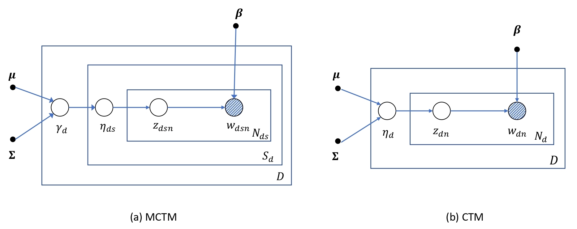
Figure 1: Graphical representations of MCTM (left) and CTM (right). The plates represent the replications of the same structure. The shaded nodes, unshaded nodes and black dots denote observed variables, hidden variables and hyperparameters, respectively.

The corresponding graphical representation of MCTM is shown in Figure 1. The plates are used to represent the replications of the same structure. The shaded nodes, unshaded nodes and black dots denote observed variables, hidden variables and hyperparameters, respectively. Here we denote $\bm{\beta}_{W\times K}=(\beta_{wz})_{W\times K}$, where $\beta_{wz}=\Pr(w_{dsn}=w|z_{dsn}=z)$ for any $d,s$ and $n$. $\bm{\gamma}$ and $\bm{z}$ are hidden variables. $v_{S}$, $v_{N}$, $\bm{\mu}$, $\bm{\Sigma}$ and $\bm{\eta}$ are hyperparameters. In practice, we see paragraphs as different segments. As ³³ pointed out, variables $\{N_{ds}\}_{d,s}$ are independent with all the other variables and we can observe $\{N_{ds}\}_{d,s}$ as well. Therefore without the loss of generality, the randomness $\{N_{ds}\}_{d,s}$ can be ignored. The topic $z_{dsn}$ corresponding to word $w_{dsn}$ given $\bm{\eta}_{ds}$ is generated from a categorical distribution with parameter $f(\bm{\eta}_{ds})$, where its $k$-th component

$$f^{(k)}(\bm{\eta}_{ds})=\frac{\exp(\eta_{dsk})}{\sum_{k=1}^{K}\exp(\eta_{dsk})},k=1,\ldots,K.$$ (1)

Given the hyperparameters $\bm{\mu}$, $\Sigma$ and $\bm{\beta}$, the joint distribution of the document-level topic mixture parameters $\bm{\gamma}=\{\bm{\gamma}_{d}\}_{d=1}^{D}$, the segment-level topic mixture parameters $\{\bm{\eta}_{ds}\}_{d,s}$, the word topics $\bm{z}=\{z_{dsn}\}_{d,s,n}$ and the observed words $\bm{w}=\{w_{dsn}\}_{d,s,n}$ is

$$p(\bm{\gamma},\bm{\eta},\bm{z},\bm{w}|\bm{\mu},\bm{\Sigma},\bm{\beta})=\prod_{d=1}^{D}p(\bm{\gamma}_{d}|\bm{\mu},\bm{\Sigma})\prod_{s=1}^{S_{d}}p(\bm{\eta}_{ds}|\bm{\gamma}_{d},\bm{\Sigma})\prod_{n=1}^{N_{sd}}p(z_{dsn}|\bm{\eta}_{ds})p(w_{dsn}|\bm{\beta},z_{dsn}).$$ (2)

The novel point of MCTM is that we consider one more layer than the CTM, which adds additional flexibility for the topic model, making it adapted to the nuanced analysis of a document in almost no more effort. More precisely, each segment has its parameter $\bm{\eta}_{ds}$ to describe the topic distribution within that segment, which is expected to capture better the local topic distribution than the global parameter $\bm{\gamma}_{d}$. Simultaneously, MCTM does not require more hyperparameters than CTM because each segment uses that document’s information to generate its parameter $\bm{\eta}_{ds}$. As mentioned in the last section, MCTM enjoys analogous spirits with the famous random effect model ²¹. For each individual, the fixed population effect is the same, while the individual effect is random. Here we can see each document as a population and segments as individuals.

It is essential to point out that MCTM can be of any depth if we pass the mean parameter of logistic normal distribution through each layer. It allows us to extend MCTM to more sophisticated structures such as the sentence-level topic model. In the following, we only consider MCTM exhibited in Figure 1 with one more layer than CTM and leave the arbitrarily deep models to future research.

3 Inference

With the Bayesian model in hand, the next step is to develop the inference algorithm. The inference goal is to estimate the parameters in the model and compute the posterior, which is very useful in future prediction and model evaluation.

In many cases, especially for complicated models, it is impossible to carry out the exact inference. We have to rely on the Bayesian approximation approaches. There are three main families of approximation methods, including Markov Chain Monte Carlo (MCMC) ²⁹, variational inference (VI) ³ and expectation propagation ²⁵. With MCMC and joint distribution, we can make the inference from complicated models. The calculation can be further simplified if the conjugacy holds. Among the MCMC family, one popular approach is Gibbs sampler ⁹. Gibbs sampler is available when the complete conditional distribution is known, which does not require the information about the joint distribution ³³. Besides, the conditional conjugacy is easier to be satisfied than the joint conjugacy ².

VI is another family of Bayesian approximation methods ¹⁷, ³⁴, which is an efficient inference method. It optimizes Kullback-Leibler (KL) divergence between exact posterior and the approximate one ³. The simplest approximation family is the mean-field family, where it is assumed that all hidden variables are independent conditioned on observed data. The parameters used to describe the independent conditional distribution of hidden variables are called variational parameters. When the conditional conjugate priors are available, the coordinate ascent VI can be straightforward to conduct. ³, and ¹² discussed the relationship between the stepwise updates and the conditional posterior under the exponential family. There has been a myriad of variants of VI appearing in recent years, including the stochastic VI ¹², the automatic differentiation VI ¹⁹, ²⁰, and black box VI ²⁷. Variational Expectation-Maximization (EM) algorithm also belongs to this family. It estimates the variational parameters and hyperparameters in two stages.

In this work, we follow similar steps of ⁵ to develop the variational EM algorithm and update the estimates through the coordinate ascent algorithm. Denote the number of topics $K$ and documents $\{\bm{w}_{d}\}_{d=1}^{D}$. Suppose the $d$-th document has $S_{d}$ segments. We are going to estimate the posterior $p(\bm{\gamma},\bm{\eta},\bm{z}|\bm{\mu},\bm{\Sigma},\bm{\beta},\bm{w})$. Consider the mean-field variational family, where we approximate the posterior with

$$q(\bm{\gamma},\bm{\eta},\bm{z}|\bm{\lambda},\bm{v}^{2},\bm{\xi},\bm{m}^{2},\bm{\phi})=\prod_{d=1}^{D}\prod_{k=1}^{K}q(\gamma_{dk}|\lambda_{dk},v_{dk}^{2})\prod_{d=1}^{D}\prod_{s=1}^{S_{d}}\prod_{k=1}^{K}q(\eta_{dsk}|\xi_{dsk},m_{dsk}^{2})\cdot\prod_{d=1}^{D}\prod_{s=1}^{S_{d}}\prod_{n=1}^{N_{ds}}q(z_{dsn}|\phi_{dsn}),$$ (3)

where $\gamma_{dk}\sim N(\lambda_{dk},v_{dk}^{2})$, $\eta_{dsk}\sim N(\xi_{dsk},m_{dsk}^{2})$ and $z_{dsn}\sim\textup{Multinomial}(\phi_{dsn})$. And $\bm{\gamma},\bm{\eta},\bm{z}$ are independent. The joint distribution of hidden variables

$$p(\bm{\gamma},\bm{\eta},\bm{z},\bm{w}|\bm{\mu},\bm{\Sigma},\bm{\beta}) =\prod_{d=1}^{D}p(\bm{\gamma}_{d}|\bm{\mu},\bm{\Sigma})\prod_{s=1}^{S_{d}}p(\bm{\eta}_{ds}|\bm{\gamma}_{d},\bm{\Sigma})\prod_{n=1}^{N_{sd}}p(z_{dsn}|\bm{\eta}_{ds})p(w_{dsn}|\bm{\beta},z_{dsn})$$ (4)

$$=\prod_{d=1}^{D}\frac{1}{(2\pi)^{\frac{K}{2}}|\bm{\Sigma}|^{\frac{1}{2}}}\exp\left\{-\frac{1}{2}(\bm{\gamma}_{d}-\bm{\mu})^{T}\bm{\Sigma}^{-1}(\bm{\gamma}_{d}-\bm{\mu})\right\}\prod_{s=1}^{S_{d}}\frac{1}{(2\pi)^{\frac{K}{2}}|\bm{\Sigma}|^{\frac{1}{2}}}\exp\left\{-\frac{1}{2}(\bm{\eta}_{ds}-\bm{\gamma}_{d})^{T}\bm{\Sigma}^{-1}(\bm{\eta}_{ds}-\bm{\gamma}_{d})\right\}\times$$ (5)

$$\quad\prod_{n=1}^{N_{sd}}\prod_{k=1}^{K}\left[f^{(k)}(\bm{\eta}_{ds})\right]^{z_{dsn}^{(k)}}\prod_{w=1}^{W}\beta_{wk}^{z_{dsn}^{(k)}}.$$ (6)

In the E-step, we are going to find the estimate of $(\bm{\lambda},\bm{v}^{2},\bm{\xi},\bm{m}^{2},\bm{\phi})$ to maximize the ELBO

$$\textup{E}_{q}[\log p(\bm{\gamma},\bm{\eta},\bm{z},\bm{w}|\bm{\mu},\bm{\Sigma},\bm{\beta})]-\textup{E}_{q}[q(\bm{\gamma},\bm{\eta},\bm{z}|\bm{\lambda},\bm{v}^{2},\bm{\xi},\bm{m}^{2},\bm{\phi})],$$ (7)

which is shown to be a lower bound of the evidence $\sum_{d=1}^{D}\log p(\bm{w}_{d}|\bm{\mu},\bm{\Sigma},\bm{\beta})$ ³. The exact ELBO is still challenging to calculate, therefore we are going to find a lower bound of it and optimize the lower bound instead ⁵. To do this, we need to define additional variational parameters $\bm{\zeta}=\{\zeta_{ds}\}_{d,s=1}$. With some straightforward calculations, it can be shown that

$$B(\bm{\mu},\bm{\Sigma},\bm{\beta},\bm{\lambda},\bm{v}^{2},\bm{\xi},\bm{m}^{2},\bm{\phi}) =-\frac{D}{2}\log|\bm{\Sigma}|-\frac{KD}{2}\log 2\pi-\frac{1}{2}\textup{Tr}(diag(\bm{v}_{d}^{2})\bm{\Sigma}^{-1})-\frac{1}{2}\sum_{d=1}^{D}(\bm{\lambda}_{d}-\bm{\mu})^{T}\bm{\Sigma}^{-1}(\bm{\lambda}_{d}-\bm{\mu})-\frac{1}{2}(K\log 2\pi+\log|\bm{\Sigma}|)\cdot\sum_{d=1}^{D}S_{d}$$ (8)

$$\quad-\frac{1}{2}\sum_{d=1}^{D}\sum_{s=1}^{S_{d}}\textup{Tr}(diag(\bm{v}_{d}^{2}+m_{ds}^{2})\bm{\Sigma}^{-1})-\frac{1}{2}\sum_{d=1}^{D}\sum_{s=1}^{S_{d}}(\bm{\xi}_{ds}-\bm{\lambda}_{d})^{T}\bm{\Sigma}^{-1}(\bm{\xi}_{ds}-\bm{\lambda}_{d})$$ (9)

$$\quad+\sum_{d=1}^{D}\sum_{s=1}^{S_{d}}\sum_{n=1}^{N_{ds}}\left[\sum_{k=1}^{K}\xi_{dsk}\phi_{dsnk}-\zeta_{ds}^{-1}\sum_{k=1}^{K}\exp(\xi_{dsk}+\frac{1}{2}m^{2}_{dsk})+1-\log\zeta_{ds}\right]+\sum_{d=1}^{D}\sum_{s=1}^{S_{d}}\sum_{n=1}^{N_{ds}}\sum_{k=1}^{K}\phi_{dsnk}\log\beta_{w_{dsn},k}$$ (10)

$$\quad+\frac{1}{2}\sum_{d=1}^{D}\sum_{k=1}^{K}(\log v_{dk}^{2}+\log 2\pi+1)+\frac{1}{2}\sum_{d=1}^{D}\sum_{s=1}^{S_{d}}\sum_{n=1}^{N_{ds}}\sum_{k=1}^{K}(\log m_{dks}^{2}+\log 2\pi+1)-\sum_{d=1}^{D}\sum_{s=1}^{S_{d}}\sum_{n=1}^{N_{ds}}\sum_{k=1}^{K}\phi_{dsnk}$$ (11)

$$\quad-\sum_{d=1}^{D}\sum_{s=1}^{S_{d}}\sum_{n=1}^{N_{ds}}\sum_{k=1}^{K}\phi_{dsnk}\log\phi_{dsnk}$$ (12)

$$\leq\textup{E}_{q}[\log p(\bm{\gamma},\bm{\eta},\bm{z},\bm{w}|\bm{\mu},\bm{\Sigma},\bm{\beta})]-\textup{E}_{q}[q(\bm{\gamma},\bm{\eta},\bm{z}|\bm{\lambda},\bm{v}^{2},\bm{\xi},\bm{m}^{2},\bm{\phi})]$$ (13)

$$\leq\sum_{d=1}^{D}\log p(\bm{w}_{d}|\bm{\mu},\bm{\Sigma},\bm{\beta}).$$ (14)

The coordinate ascent algorithm can be easily conducted through stepwise optimization of $B(\bm{\mu},\bm{\Sigma},\bm{\beta},\bm{\lambda},\bm{v}^{2},\bm{\xi},\bm{m}^{2},\bm{\phi})$. The updating formulas of estimate $(\hat{\zeta}_{ds},\hat{\phi}_{dsnk},\hat{\bm{\lambda}}_{d},\hat{v}_{dk})$ are

$$\hat{\zeta}_{ds} =\sum_{k=1}^{K}\exp\left\{\hat{\xi}_{dsk}+\frac{1}{2}\hat{m}_{dsk}^{2}\right\},$$ (15)

$$\hat{\phi}_{dsnk} \propto\beta_{w_{dsn},k}\exp\{\hat{\xi}_{dsk}\},k=1,\ldots,K,$$ (16)

$$\hat{\bm{\lambda}}_{d} =(S_{d}+1)^{-1}\left(\sum_{s=1}^{S_{d}}\hat{\bm{\xi}}_{ds}+\bm{\mu}\right),$$ (17)

$$\hat{v}_{dk} =((S_{d}+1)(\bm{\Sigma}^{-1})_{kk})^{-1}.$$ (18)

For $\bm{\xi}$, $\bm{m}$, we find their estimates through Newton-Raphson algorithm. The corresponding gradient and hessian matrix are

$$\nabla_{\bm{\xi}_{ds}}B =-\bm{\Sigma}^{-1}(\bm{\xi}_{ds}-\bm{\lambda}_{d})+\sum_{n=1}^{N_{ds}}\bm{\phi}_{dsn}-\frac{N_{ds}}{\zeta_{ds}}\exp\left\{\bm{\xi}_{ds}+\frac{1}{2}\bm{m}_{ds}^{2}\right\},$$ (19)

$$\nabla_{\bm{\xi}_{ds}}^{2}B =-\bm{\Sigma}^{-1}-\frac{N_{ds}}{\zeta_{ds}}\textup{diag}\left(\exp\left\{\bm{\xi}_{ds}+\frac{1}{2}\bm{m}_{ds}^{2}\right\}\right),$$ (20)

$$\frac{\partial B}{\partial m_{dsk}^{2}} =-\frac{1}{2}(\Sigma^{-1})_{kk}-\frac{N_{ds}}{2\zeta_{ds}}\exp\left\{\bm{\xi}_{ds}+\frac{1}{2}\bm{m}_{ds}^{2}\right\}+\frac{1}{2m_{dsk}^{2}},$$ (21)

$$\frac{\partial^{2}B}{\partial(m_{dsk}^{2})^{2}} =-\frac{N_{ds}}{4\zeta_{ds}}\exp\left\{\bm{\xi}_{ds}+\frac{1}{2}\bm{m}_{ds}^{2}\right\}-\frac{1}{2m_{dsk}^{4}}.$$ (22)

In the M-step, we update the hyperparameters $(\bm{\mu},\Sigma,\bm{\beta})$ to maximize $B(\bm{\mu},\bm{\Sigma},\bm{\beta},\bm{\lambda},\bm{v}^{2},\bm{\xi},\bm{m}^{2},\bm{\phi})$ each step by

$$\hat{\beta}_{wk} \propto\sum_{d=1}^{D}\sum_{s=1}^{S_{d}}\#\{n:w_{sdn}=w\}\hat{\phi}_{dsnk},$$ (23)

$$\hat{\bm{\mu}} =\frac{1}{D}\sum_{d=1}^{D}\hat{\bm{\lambda}}_{d},$$ (24)

$$\hat{\bm{\Sigma}} =\frac{1}{D+\sum_{d=1}^{D}S_{d}}\cdot\left[\sum_{d=1}^{D}\textup{diag}(\hat{\bm{v}}_{d}^{2})+\sum_{d=1}^{D}\sum_{s=1}^{S_{d}}\textup{diag}(\hat{\bm{v}}_{d}^{2}+\hat{\bm{m}}_{ds}^{2})+\sum_{d=1}^{D}(\hat{\bm{\lambda}}_{d}-\hat{\bm{\mu}})(\hat{\bm{\lambda}}_{d}-\hat{\bm{\mu}})^{T}+\sum_{d=1}^{D}\sum_{s=1}^{S_{d}}(\hat{\bm{\xi}}_{ds}-\hat{\bm{\lambda}}_{d})(\hat{\bm{\xi}}_{ds}-\hat{\bm{\lambda}}_{d})^{T}\right].$$ (25)

The detailed derivation of the results above can be found in Appendix A.

4 Applications

In this section, we point out two potential applications, including paragraph-level document analysis and market basket analysis, where MCTM can be directly applied. The experiment results on these two problems will be presented in the next section.

4.1 Paragraph-level document analysis

As mentioned in Section 1, the original LDA model ⁶ and CTM ⁵ conducted only the document-level topic analysis, which assume the interchangeability of words within each document. MCTM relaxes this assumption by only requiring the interchangeability within each segment. In practice, each paragraph is natural to be a segment. An article has some main ideas, and each paragraph of it is organized and can carry out slightly different information around these ideas ⁸. Understanding what each paragraph of an article is talking about can be very useful in text mining.

4.2 Market basket analysis

The decision process that consumers select items from various products in the same shopping trip is called a market basket choice problem ³², ³¹. Numerous models have been developed to analyze market basket data. ¹⁵ fitted LDA and CTM on market basket data and obtained some interesting conclusions. Although the topic models might not be favorable in dealing with the market basket data ¹⁶, it is helpful for us to explore the common shopping pattern and the preference of each customer via topic models. The topic models’ results could help the market design better promotion strategies and recommend appropriate products to customers.

We can adapt MCTM into the market basket analysis with no extra efforts. Items can be seen as different words in document analysis. Each topic indicates a specific shopping pattern of these items. Consider different customers $d=1,\ldots D$ and the $d$-th customer has $s=1,\ldots,S_{d}$ shopping trips in total. Within the $s$-th trip of customer $d$, a list of items $w_{ds1},\ldots,w_{dsN_{ds}}$ are added into the cart. Each customer can be seen as a “document,” and each trip can be seen as a “segment”. The data generation procedure is the same as presented in Section 2. The corresponding variational EM algorithm presented in Section 3 can be immediately applied.

5 Experimental Results

5.1 NIPS dataset

We first demonstrate the effectiveness of MCTM to capture the local structure of articles in paragraph-level document analysis. We take NIPS conference papers published during 2015-2017 as the dataset. We removed all the words appearing for less than three times and all the paragraphs with less than 20 words. Also, we used a list of scientific stop words and common stop words from ISO dataset provided by the R package stopwords. Finally, the NIPS dataset contains 1646 documents with 1181156 words. There are 20667 unique words in total.

We evaluate different models by investigating the perplexity. Define the training set as $\bm{w}_{\textup{train}}$ and the parameters fitted using the training set are $\Upsilon$. Denote the held-out documents as $\bm{w}_{\textup{held-out}}=\{\bm{w}_{d}\}_{d=1}^{D}$ and suppose $\bm{w}_{d}$ has $N_{d}$ words in total. Then we define the perplexity as

$$\textup{Perplexity}=\left(\prod_{d=1}^{D}\textup{P}(\bm{w}_{d}|\Upsilon,\bm{w}_{\textup{train}})\right)^{-1/(\sum_{d=1}^{D}N_{d})}.$$ (26)

The lower perplexity denotes a more powerful model. In experiments, it is estimated by following the harmonic mean method and treating the approximate posteriors as the real proposed ones ³⁶.

We used the 2016-2017 NIPS papers, which contains 1244 documents and 930588 words in total, as the training set. The 2015 NIPS papers, which contains 402 documents and 250568 words, are used as held-out documents. We fitted the LDA model ⁶, CTM ⁵ and MCTM by considering 10, 20, 30, 40, 50, 60, 70, 80 topics. The LDA model and CTM are implemented by R package topicmodels ¹³. The inference algorithm is run until the relative change of ELBO or the lower bound of ELBO is less than 0.0001%.

topic 1	topic 2	topic 3	topic 4	topic 5	topic 6	topic 7	topic 8	topic 9
“optimization"	“classification"	“memory"	“image processing"	“graph"	“bound"	“kernel"	“online learning"	“acknowledgment"
gradient	loss	size	images	graph	bound	kernel	regret	supported
vector	classifier	memory	image	nodes	bounds	kernels	algorithms	grant
optimization	classifiers	compression	layers	node	upper	space	online	nsf
loss	examples	bit	dataset	edges	bounded	gaussian	bandit	acknowledgments
descent	binary	quantization	neural	graphs	inequality	rkhs	action	reward
step	risk	values	networks	vertices	holds	hilbert	reward	agent
iteration	hinge	cost	convolutional	clustering	tight	functions	learner	university
functions	losses	datasets	architecture	tree	terms	reproducing	actions	tasks
respect	decision	dataset	features	algorithms	implies	matrix	settings	policies
approximation	neural	hash	size	sets	constants	features	unknown	neural

Table 1: Top 10 words with highest frequency from 9 selected topics. The results is obtained from a 40-topic MCTM.

First, we presented 9 topics with the corresponding top 10 words with the highest frequency derived from the training data by fitting a 40-topic MCTM in Table 1. Notice that MCTM indeed captures the hidden structure of the documents, and these topics are interpretable. Notice that there is a special topic, which we call “acknowledgment", including some words often used in the acknowledgment paragraph. Our model can capture this topic because of its hierarchical structure and flexible variation between documents and paragraphs. To intuitively show how MCTM captures the difference between topics of different paragraphs, we take the following example. Figure 2 shows the last paragraph of 2017 NIPS paper “On clustering network-valued data" ²⁶. This paper is one of the training documents, and we highlight the training words in this paragraph. This paragraph’s approximate posterior topic distribution shows that in 96.6% probability, a word is generated from the “acknowledgment" topic. While in the whole paper, this probability is only 0.0027%. Capturing the difference between the document-level topic proportion and paragraph-level proportion leads to the success of MCTM when we are interested in the local structure of an article.

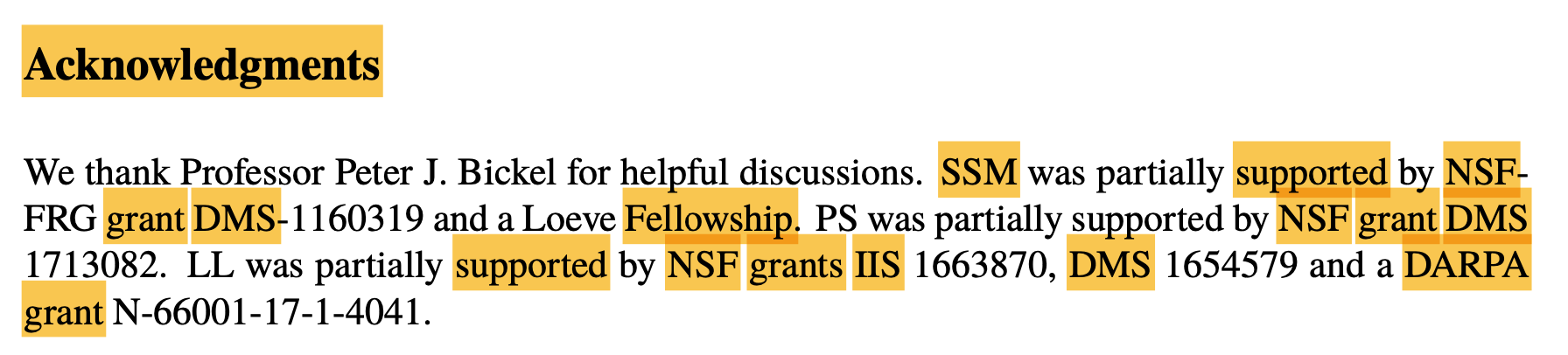
Figure 2: The last paragraph of 2017 NIPS paper “On clustering network-valued data". Training words are highlighted. In this paragraph the “acknowledgement" topic proportion is 96.6% while in the whole paper it is only 0.0027%.

Next, we presented the perplexity with respect to different numbers of topics $K$ in Figure 3. From the results it can be observed that LDA and CTM achieve comparable performance while MCTM outperforms both of them. This is because MCTM can capture more sophisticated document structure which LDA and CTM cannot describe.

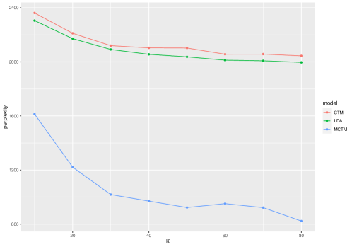
Figure 3: Perplexity of LDA, CTM and MCTM with respect to different number of topics and percentage of observed words in held-out documents.

Finally, we visualize the results of MCTM by constructing an intuitive figure of the document “On clustering network-valued data" with its several paragraphs and topics. It is exhibited as Figure 4. Each circle represents a paragraph of the document with 5 highest-frequency words in that paragraph, while each rectangle denotes a topic with 5 top words. We connect the document and its paragraphs with topics achieving over $1\%$ proportion level. It can be observed that the document has connections with topics 2, 11, 15, 27, and 34, while some paragraphs only focus on some of them. For instance, paragraph 4 discusses mainly the “graph” and “matrix”. All six paragraphs are connected with topic 11 “graph”, which is the whole document’s focus. Besides, paragraph 21 only connects with topic 11 “graph” and topic 32 “acknowledgment”. We have shown this paragraph in Figure 2, and it is an acknowledgment paragraph. Such a figure can be immediately drawn for each document after fitting MCTM, which clearly shows the local structure.

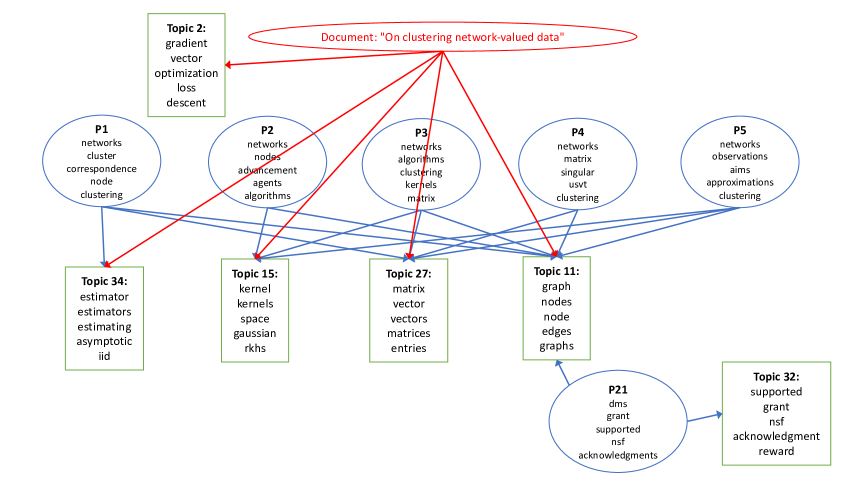
Figure 4: Document “On clustering network-valued data" with its several paragraphs and some topics. The document and its paragraphs are connected with topics achieving over $1\%$ proportion level.

5.2 Instacart market basket dataset

In this section, we apply MCTM to study the market basket data by following the idea described in Section 4.2. The dataset we used is the shopping data provided by Instacart, a big grocery market in the United States and Canada. It consists of the records of over 200000 customers. We take the first 1000 customers, coupled with 15145 trips and 150150 bought items as our training data. On each trip, the customer bought at least four items. There are 134 different categories to which the products belong. We fit MCTM based on these categories instead of single items.

topic 1	topic 2	topic 3	topic 4	topic 5
“laundry and other household"	“baby and body care"	“frozen products"	“vegetable, fruits and milk"	"drinking and body care"
laundry	baby food formula	frozen meals	fresh vegetables	body lotions soap
deodorants	diapers wipes	frozen breakfast	fresh fruits	beers coolers
mint gum	baby bath body care	frozen pizza	packaged vegetables fruits	muscles joints pain relief
cleaning products	energy granola bars	instant foods	yogurt	dog food care
dish detergents	fruit vegetable snacks	cereal	packaged cheese	white wines
trash bags liners	laundry	frozen appetizers sides	chips pretzels	air fresheners candles
oral hygiene	canned fruit applesauce	plates bowls cups flatware	water seltzer sparkling water	ice cream toppings
baby accessories	food storage	frozen dessert	frozen produce	red wines
more household	cereal	frozen vegan vegetarian	ice cream ice	first aid
paper goods	hair care	hair care	milk	spirits

Table 2: 5 selected topics and the corresponding top 10 categories from derived from a 20-topic MCTM.

We fitted a 20-topic MCTM and presented 5 topics and corresponding top 10 categories in Table 2. Observe that the MCTM successfully captures some shopping needs, including the household, baby care, body care, frozen products, vegetables, and drinking. Besides, by looking at each customer’s topic proportion, we can better know the categories each customer often buys, which helps analyze each consumer’s preference and promote the right products to them. The analysis of individual customers’ behavior is out of our discussion scope, and we do not cover it here.

6 Discussion

In this work, we proposed an innovative multilayer correlated topic model (MCTM) to analyze the documents’ local structure. It is motivated by the connection between articles published at different times in the dynamic topic model ⁴ and the group structure used in the random effect model ²¹. The variational EM algorithm, coupled with MCTM, was derived for posterior and parameter estimation. We introduced two potential applications of MCTM, including the paragraph-level document analysis and market basket data analysis. In numerical studies, we demonstrated the effectiveness of MCTM in capturing the document structure, and MCTM was confirmed to improve LDA and CTM. We visualized the relationship between the main ideas of a document and its paragraphs. Besides, we captured some hidden shopping patterns among customers by applying MCTM on market basket data.

Our work’s main contribution is that we developed a very natural and straightforward way to extend CTM ⁵ in almost no extra effort, making it possible to capture the heterogeneity between paragraphs of a document. Understanding the local structure of an article can help investigate how central ideas are organized inside a document.

There are a few future avenues that are interesting to explore. The first one is the usage of the covariance matrix in the logistic normal distribution. As ⁵ suggested, the covariance can help analyze the pairwise correlation between different topics. Similar results can be obtained for MCTM as well. Besides, in our framework, topics do not have to share the same correlation structure at different levels. Using separate covariance matrices at different levels might help interpret the relationship between a document and its paragraphs. Second, as we mentioned before, MCTM can be of any depth, making it ready to be extended for more sophisticated modeling such as the sentence-level topic modeling. Another appealing direction is to look for better ways to visualize the results of MCTM. Figure 4 provides a good example, and we expect to see more intuitive visualization methods to display the results.

Data accessibility

The NIPS dataset is available at https://www.kaggle.com/benhamner/nips-papers, and the Instacart market basket dataset is available at https://www.kaggle.com/c/instacart-market-basket-analysis.

Appendix A Derivation of variational EM algorithm in Section 3

In this section, we treat $z_{dsn}$ as a $K$-vector as $z_{dsn}=(z_{dsn}^{(1)},\ldots,z_{dsn}^{(K)})^{T}$, where each coordinate is an indicator. For instance, if the $n$-th word in the $s$-th segment of the $d$-th document has topic $k$, then $z_{dsn}^{(j)}=\mathds{1}(j=k)$ for $j=1,\ldots,K$.

By ³, the ELBO equals to

$$\textup{E}_{q}[\log p(\bm{\gamma},\bm{\eta},\bm{z},\bm{w}|\bm{\mu},\bm{\Sigma},\bm{\beta})]-\textup{E}_{q}[q(\bm{\gamma},\bm{\eta},\bm{z}|\bm{\lambda},\bm{v}^{2},\bm{\xi},\bm{m}^{2},\bm{\phi})].$$ (27)

Due to (6) and the normal density, we have

$$\textup{E}_{q}[\log p(\bm{\gamma}_{d}|\bm{\mu},\bm{\Sigma})] =\frac{1}{2}\log|\bm{\Sigma}|^{-1}-\frac{K}{2}\log 2\pi-\frac{1}{2}\textup{E}_{q}[(\bm{\gamma}_{d}-\bm{\mu})^{T}\bm{\Sigma}^{-1}(\bm{\gamma}_{d}-\bm{\mu})]$$ (28)

$$=-\frac{1}{2}\log|\bm{\Sigma}|-\frac{K}{2}\log 2\pi-\frac{1}{2}\textup{Tr}(\textup{diag}(\bm{v}_{d}^{2})\bm{\Sigma}^{-1})-\frac{1}{2}(\bm{\lambda}_{d}-\bm{\mu})^{T}\bm{\Sigma}^{-1}(\bm{\lambda}_{d}-\bm{\mu}).$$ (29)

Similarly, it holds that

$$\textup{E}_{q}[\log p(\bm{\eta}_{ds}|\bm{\gamma}_{d},\bm{\Sigma})] =-\frac{1}{2}\log|\bm{\Sigma}|-\frac{K}{2}\log 2\pi-\frac{1}{2}\textup{E}_{q}[(\bm{\eta}_{ds}-\bm{\gamma}_{d})^{T}\bm{\Sigma}^{-1}(\bm{\eta}_{ds}-\bm{\gamma}_{d})]$$ (30)

$$=-\frac{1}{2}\log|\bm{\Sigma}|-\frac{K}{2}\log 2\pi-\frac{1}{2}\textup{Tr}(\textup{diag}(\bm{m}_{ds}^{2}+\bm{v}_{d}^{2})\bm{\Sigma}^{-1})-\frac{1}{2}(\bm{\xi}_{ds}-\bm{\lambda}_{d})^{T}\bm{\Sigma}^{-1}(\bm{\xi}_{ds}-\bm{\lambda}_{d}).$$ (31)

According to the categorical distribution, we have

$$\textup{E}_{q}[\log p(z_{dsn}|\bm{\eta}_{ds})]=\textup{E}_{q}(\bm{\eta}_{ds}^{T}\bm{z}_{dsn})-\textup{E}_{q}\left[\log\left(\sum_{k=1}^{K}\exp(\eta_{dsk})\right)\right].$$ (32)

Since the second term does not have a close form, we follow the strategy of ⁵ by introducing additional positive parameters $\bm{\xi}=\{\xi_{ds}\}_{d,s}$. It can be easily checked that

$$\textup{E}_{q}\left[\log\left(\sum_{k=1}^{K}\exp(\eta_{dsk})\right)\right] \leq\xi_{ds}^{-1}\left[\sum_{k=1}^{K}\textup{E}_{q}(\exp(\eta_{dsk}))\right]-1+\log\xi_{ds}$$ (33)

$$=\xi_{ds}^{-1}\left[\sum_{k=1}^{K}\textup{E}_{q}\left(\exp\left(\xi_{dsk}+\frac{1}{2}m_{dsk}^{2}\right)\right)\right]-1+\log\xi_{ds},$$ (34)

where the second equality comes from the moment generating function of normal distributed $\xi_{dsk}$ under $q$. In addition, we have

$$\textup{E}_{q}[\log p(w_{dsn}|z_{dsn},\bm{\beta})]=\sum_{k=1}^{K}\phi_{dsnk}\log\beta_{w_{dsn},k}.$$ (35)

On the other hand, it holds that

$$\textup{E}_{q}[\log q(\gamma_{dk}|\lambda_{dk},v^{2}_{dk})] =-\frac{1}{2}(\log v^{2}_{dk}+\log 2\pi+1),$$ (36)

$$\textup{E}_{q}[\log q(\eta_{dsk}|\xi_{dsk},m^{2}_{dsk})] =-\frac{1}{2}(\log m^{2}_{dsk}+\log 2\pi+1),$$ (37)

$$\textup{E}_{q}[\log q(z_{dsn}|\phi_{dsn})] =\phi_{dsnk}\log\phi_{dsnk}.$$ (38)

Combining (6), (3), (29), (31), (34), (35), (36), (37), (38), it follows that ELBO can be bounded by $B(\bm{\mu},\bm{\Sigma},\bm{\beta},\bm{\lambda},\bm{v}^{2},\bm{\xi},\bm{m}^{2},\bm{\phi})$. Then the derivations exhibited in Section 3 are straightforward to obtain.

References

- Atchison \BBA Shen \APACyear1980 \APACinsertmetastaratchison1980logistic{APACrefauthors}Atchison, J.\BCBT \BBA Shen, S\BPBIM. \APACrefYearMonthDay1980. \BBOQ\APACrefatitleLogistic-normal distributions: Some properties and uses Logistic-normal distributions: Some properties and uses.\BBCQ \APACjournalVolNumPagesBiometrika672261–272. \PrintBackRefs\CurrentBib
- Blei \APACyear2014 \APACinsertmetastarblei2014build{APACrefauthors}Blei, D\BPBIM. \APACrefYearMonthDay2014. \BBOQ\APACrefatitleBuild, compute, critique, repeat: Data analysis with latent variable models Build, compute, critique, repeat: Data analysis with latent variable models.\BBCQ \PrintBackRefs\CurrentBib
- Blei \BOthers. \APACyear2017 \APACinsertmetastarblei2017variational{APACrefauthors}Blei, D\BPBIM., Kucukelbir, A.\BCBL \BBA McAuliffe, J\BPBID. \APACrefYearMonthDay2017. \BBOQ\APACrefatitleVariational inference: A review for statisticians Variational inference: A review for statisticians.\BBCQ \APACjournalVolNumPagesJournal of the American statistical Association112518859–877. \PrintBackRefs\CurrentBib
- Blei \BBA Lafferty \APACyear2006 \APACinsertmetastarblei2006dynamic{APACrefauthors}Blei, D\BPBIM.\BCBT \BBA Lafferty, J\BPBID. \APACrefYearMonthDay2006. \BBOQ\APACrefatitleDynamic topic models Dynamic topic models.\BBCQ \BIn \APACrefbtitleProceedings of the 23rd international conference on Machine learning Proceedings of the 23rd international conference on machine learning (\BPGS 113–120). \PrintBackRefs\CurrentBib
- Blei \BOthers. \APACyear2007 \APACinsertmetastarblei2007correlated{APACrefauthors}Blei, D\BPBIM., Lafferty, J\BPBID.\BCBL \BOthersPeriod. \APACrefYearMonthDay2007. \BBOQ\APACrefatitleA correlated topic model of science A correlated topic model of science.\BBCQ \APACjournalVolNumPagesThe Annals of Applied Statistics1117–35. \PrintBackRefs\CurrentBib
- Blei \BOthers. \APACyear2003 \APACinsertmetastarblei2003latent{APACrefauthors}Blei, D\BPBIM., Ng, A\BPBIY.\BCBL \BBA Jordan, M\BPBII. \APACrefYearMonthDay2003. \BBOQ\APACrefatitleLatent dirichlet allocation Latent dirichlet allocation.\BBCQ \APACjournalVolNumPagesJournal of machine Learning research3Jan993–1022. \PrintBackRefs\CurrentBib
- Boztuğ \BBA Hildebrandt \APACyear2008 \APACinsertmetastarboztuug2008modeling{APACrefauthors}Boztuğ, Y.\BCBT \BBA Hildebrandt, L. \APACrefYearMonthDay2008. \BBOQ\APACrefatitleModeling joint purchases with a multivariate MNL approach Modeling joint purchases with a multivariate mnl approach.\BBCQ \APACjournalVolNumPagesSchmalenbach Business Review604400–422. \PrintBackRefs\CurrentBib
- Du \BOthers. \APACyear2010 \APACinsertmetastardu2010segmented{APACrefauthors}Du, L., Buntine, W.\BCBL \BBA Jin, H. \APACrefYearMonthDay2010. \BBOQ\APACrefatitleA segmented topic model based on the two-parameter Poisson-Dirichlet process A segmented topic model based on the two-parameter poisson-dirichlet process.\BBCQ \APACjournalVolNumPagesMachine learning8115–19. \PrintBackRefs\CurrentBib
- Gelfand \BBA Smith \APACyear1990 \APACinsertmetastargelfand1990sampling{APACrefauthors}Gelfand, A\BPBIE.\BCBT \BBA Smith, A\BPBIF. \APACrefYearMonthDay1990. \BBOQ\APACrefatitleSampling-based approaches to calculating marginal densities Sampling-based approaches to calculating marginal densities.\BBCQ \APACjournalVolNumPagesJournal of the American statistical association85410398–409. \PrintBackRefs\CurrentBib
- Griffiths \BOthers. \APACyear2004 \APACinsertmetastargriffiths2004hierarchical{APACrefauthors}Griffiths, T\BPBIL., Jordan, M\BPBII., Tenenbaum, J\BPBIB.\BCBL \BBA Blei, D\BPBIM. \APACrefYearMonthDay2004. \BBOQ\APACrefatitleHierarchical topic models and the nested Chinese restaurant process Hierarchical topic models and the nested chinese restaurant process.\BBCQ \BIn \APACrefbtitleAdvances in neural information processing systems Advances in neural information processing systems (\BPGS 17–24). \PrintBackRefs\CurrentBib
- Guo \BOthers. \APACyear2019 \APACinsertmetastarguo2019improved{APACrefauthors}Guo, C., Lu, M.\BCBL \BBA Wei, W. \APACrefYearMonthDay2019. \BBOQ\APACrefatitleAn Improved LDA Topic Modeling Method Based on Partition for Medium and Long Texts An improved lda topic modeling method based on partition for medium and long texts.\BBCQ \APACjournalVolNumPagesAnnals of Data Science1–14. \PrintBackRefs\CurrentBib
- Hoffman \BOthers. \APACyear2013 \APACinsertmetastarhoffman2013stochastic{APACrefauthors}Hoffman, M\BPBID., Blei, D\BPBIM., Wang, C.\BCBL \BBA Paisley, J. \APACrefYearMonthDay2013. \BBOQ\APACrefatitleStochastic variational inference Stochastic variational inference.\BBCQ \APACjournalVolNumPagesThe Journal of Machine Learning Research1411303–1347. \PrintBackRefs\CurrentBib
- Hornik \BBA Grün \APACyear2011 \APACinsertmetastarhornik2011topicmodels{APACrefauthors}Hornik, K.\BCBT \BBA Grün, B. \APACrefYearMonthDay2011. \BBOQ\APACrefatitletopicmodels: An R package for fitting topic models topicmodels: An r package for fitting topic models.\BBCQ \APACjournalVolNumPagesJournal of statistical software40131–30. \PrintBackRefs\CurrentBib
- Hou \BOthers. \APACyear2017 \APACinsertmetastarhou2017multi{APACrefauthors}Hou, S., Chen, L., Tao, D., Zhou, S., Liu, W.\BCBL \BBA Zheng, Y. \APACrefYearMonthDay2017. \BBOQ\APACrefatitleMulti-layer multi-view topic model for classifying advertising video Multi-layer multi-view topic model for classifying advertising video.\BBCQ \APACjournalVolNumPagesPattern Recognition6866–81. \PrintBackRefs\CurrentBib
- Hruschka \APACyear2014 \APACinsertmetastarhruschka2014linking{APACrefauthors}Hruschka, H. \APACrefYearMonthDay2014. \BBOQ\APACrefatitleLinking multi-category purchases to latent activities of shoppers: analysing market baskets by topic models Linking multi-category purchases to latent activities of shoppers: analysing market baskets by topic models.\BBCQ \APACjournalVolNumPagesMarketing: ZFP–Journal of Research and Management364267–273. \PrintBackRefs\CurrentBib
- Hruschka \APACyear2019 \APACinsertmetastarhruschka2019comparing{APACrefauthors}Hruschka, H. \APACrefYearMonthDay2019. \BBOQ\APACrefatitleComparing unsupervised probabilistic machine learning methods for market basket analysis Comparing unsupervised probabilistic machine learning methods for market basket analysis.\BBCQ \APACjournalVolNumPagesReview of Managerial Science1–31. \PrintBackRefs\CurrentBib
- Jordan \BOthers. \APACyear1999 \APACinsertmetastarjordan1999introduction{APACrefauthors}Jordan, M\BPBII., Ghahramani, Z., Jaakkola, T\BPBIS.\BCBL \BBA Saul, L\BPBIK. \APACrefYearMonthDay1999. \BBOQ\APACrefatitleAn introduction to variational methods for graphical models An introduction to variational methods for graphical models.\BBCQ \APACjournalVolNumPagesMachine learning372183–233. \PrintBackRefs\CurrentBib
- Kraus \BBA Feuerriegel \APACyear2019 \APACinsertmetastarkraus2019personalized{APACrefauthors}Kraus, M.\BCBT \BBA Feuerriegel, S. \APACrefYearMonthDay2019. \BBOQ\APACrefatitlePersonalized Purchase Prediction of Market Baskets with Wasserstein-Based Sequence Matching Personalized purchase prediction of market baskets with wasserstein-based sequence matching.\BBCQ \BIn \APACrefbtitleProceedings of the 25th ACM SIGKDD International Conference on Knowledge Discovery & Data Mining Proceedings of the 25th acm sigkdd international conference on knowledge discovery & data mining (\BPGS 2643–2652). \PrintBackRefs\CurrentBib
- Kucukelbir \BOthers. \APACyear2015 \APACinsertmetastarkucukelbir2015automatic{APACrefauthors}Kucukelbir, A., Ranganath, R., Gelman, A.\BCBL \BBA Blei, D. \APACrefYearMonthDay2015. \BBOQ\APACrefatitleAutomatic variational inference in Stan Automatic variational inference in stan.\BBCQ \APACjournalVolNumPagesAdvances in neural information processing systems28568–576. \PrintBackRefs\CurrentBib
- Kucukelbir \BOthers. \APACyear2017 \APACinsertmetastarkucukelbir2017automatic{APACrefauthors}Kucukelbir, A., Tran, D., Ranganath, R., Gelman, A.\BCBL \BBA Blei, D\BPBIM. \APACrefYearMonthDay2017. \BBOQ\APACrefatitleAutomatic differentiation variational inference Automatic differentiation variational inference.\BBCQ \APACjournalVolNumPagesThe Journal of Machine Learning Research181430–474. \PrintBackRefs\CurrentBib
- Laird \BBA Ware \APACyear1982 \APACinsertmetastarlaird1982random{APACrefauthors}Laird, N\BPBIM.\BCBT \BBA Ware, J\BPBIH. \APACrefYearMonthDay1982. \BBOQ\APACrefatitleRandom-effects models for longitudinal data Random-effects models for longitudinal data.\BBCQ \APACjournalVolNumPagesBiometrics963–974. \PrintBackRefs\CurrentBib
- Li \BOthers. \APACyear2020 \APACinsertmetastarli2020context{APACrefauthors}Li, W., Matsukawa, T., Saigo, H.\BCBL \BBA Suzuki, E. \APACrefYearMonthDay2020. \BBOQ\APACrefatitleContext-Aware Latent Dirichlet Allocation for Topic Segmentation Context-aware latent dirichlet allocation for topic segmentation.\BBCQ \BIn \APACrefbtitlePacific-Asia Conference on Knowledge Discovery and Data Mining Pacific-asia conference on knowledge discovery and data mining (\BPGS 475–486). \PrintBackRefs\CurrentBib
- Li \BBA McCallum \APACyear2006 \APACinsertmetastarli2006pachinko{APACrefauthors}Li, W.\BCBT \BBA McCallum, A. \APACrefYearMonthDay2006. \BBOQ\APACrefatitlePachinko allocation: DAG-structured mixture models of topic correlations Pachinko allocation: Dag-structured mixture models of topic correlations.\BBCQ \BIn \APACrefbtitleProceedings of the 23rd international conference on Machine learning Proceedings of the 23rd international conference on machine learning (\BPGS 577–584). \PrintBackRefs\CurrentBib
- McCallum \APACyear1999 \APACinsertmetastarmccallum1999multi{APACrefauthors}McCallum, A\BPBIK. \APACrefYearMonthDay1999. \BBOQ\APACrefatitleMulti-label text classification with a mixture model trained by EM Multi-label text classification with a mixture model trained by em.\BBCQ \BIn \APACrefbtitleAAAI 99 workshop on text learning. Aaai 99 workshop on text learning. \PrintBackRefs\CurrentBib
- Minka \APACyear2013 \APACinsertmetastarminka2013expectation{APACrefauthors}Minka, T\BPBIP. \APACrefYearMonthDay2013. \BBOQ\APACrefatitleExpectation propagation for approximate Bayesian inference Expectation propagation for approximate bayesian inference.\BBCQ \APACjournalVolNumPagesarXiv preprint arXiv:1301.2294. \PrintBackRefs\CurrentBib
- Mukherjee \BOthers. \APACyear2017 \APACinsertmetastarmukherjee2017clustering{APACrefauthors}Mukherjee, S\BPBIS., Sarkar, P.\BCBL \BBA Lin, L. \APACrefYearMonthDay2017. \BBOQ\APACrefatitleOn clustering network-valued data On clustering network-valued data.\BBCQ \BIn \APACrefbtitleAdvances in neural information processing systems Advances in neural information processing systems (\BPGS 7071–7081). \PrintBackRefs\CurrentBib
- Ranganath \BOthers. \APACyear2014 \APACinsertmetastarranganath2014black{APACrefauthors}Ranganath, R., Gerrish, S.\BCBL \BBA Blei, D. \APACrefYearMonthDay2014. \BBOQ\APACrefatitleBlack box variational inference Black box variational inference.\BBCQ \BIn \APACrefbtitleArtificial Intelligence and Statistics Artificial intelligence and statistics (\BPGS 814–822). \PrintBackRefs\CurrentBib
- Reisenbichler \BBA Reutterer \APACyear2019 \APACinsertmetastarreisenbichler2019topic{APACrefauthors}Reisenbichler, M.\BCBT \BBA Reutterer, T. \APACrefYearMonthDay2019. \BBOQ\APACrefatitleTopic modeling in marketing: recent advances and research opportunities Topic modeling in marketing: recent advances and research opportunities.\BBCQ \APACjournalVolNumPagesJournal of Business Economics893327–356. \PrintBackRefs\CurrentBib
- Robert \BBA Casella \APACyear2013 \APACinsertmetastarrobert2013monte{APACrefauthors}Robert, C.\BCBT \BBA Casella, G. \APACrefYear2013. \APACrefbtitleMonte Carlo statistical methods Monte carlo statistical methods. \APACaddressPublisherSpringer Science & Business Media. \PrintBackRefs\CurrentBib
- Rosen-Zvi \BOthers. \APACyear2012 \APACinsertmetastarrosen2012author{APACrefauthors}Rosen-Zvi, M., Griffiths, T., Steyvers, M.\BCBL \BBA Smyth, P. \APACrefYearMonthDay2012. \BBOQ\APACrefatitleThe author-topic model for authors and documents The author-topic model for authors and documents.\BBCQ \APACjournalVolNumPagesarXiv preprint arXiv:1207.4169. \PrintBackRefs\CurrentBib
- Russell \BBA Petersen \APACyear2000 \APACinsertmetastarrussell2000analysis{APACrefauthors}Russell, G\BPBIJ.\BCBT \BBA Petersen, A. \APACrefYearMonthDay2000. \BBOQ\APACrefatitleAnalysis of cross category dependence in market basket selection Analysis of cross category dependence in market basket selection.\BBCQ \APACjournalVolNumPagesJournal of Retailing763367–392. \PrintBackRefs\CurrentBib
- Russell \BOthers. \APACyear1999 \APACinsertmetastarrussell1999multiple{APACrefauthors}Russell, G\BPBIJ., Ratneshwar, S., Shocker, A\BPBID., Bell, D., Bodapati, A., Degeratu, A.\BDBLShankar, V\BPBIH. \APACrefYearMonthDay1999. \BBOQ\APACrefatitleMultiple-category decision-making: Review and synthesis Multiple-category decision-making: Review and synthesis.\BBCQ \APACjournalVolNumPagesMarketing Letters103319–332. \PrintBackRefs\CurrentBib
- Shafiei \BBA Milios \APACyear2006 \APACinsertmetastarshafiei2006latent{APACrefauthors}Shafiei, M\BPBIM.\BCBT \BBA Milios, E\BPBIE. \APACrefYearMonthDay2006. \BBOQ\APACrefatitleLatent Dirichlet co-clustering Latent dirichlet co-clustering.\BBCQ \BIn \APACrefbtitleSixth International Conference on Data Mining (ICDM’06) Sixth international conference on data mining (icdm’06) (\BPGS 542–551). \PrintBackRefs\CurrentBib
- Wainwright \BBA Jordan \APACyear2008 \APACinsertmetastarwainwright2008graphical{APACrefauthors}Wainwright, M\BPBIJ.\BCBT \BBA Jordan, M\BPBII. \APACrefYear2008. \APACrefbtitleGraphical models, exponential families, and variational inference Graphical models, exponential families, and variational inference. \APACaddressPublisherNow Publishers Inc. \PrintBackRefs\CurrentBib
- Wallach \APACyear2006 \APACinsertmetastarwallach2006topic{APACrefauthors}Wallach, H\BPBIM. \APACrefYearMonthDay2006. \BBOQ\APACrefatitleTopic modeling: beyond bag-of-words Topic modeling: beyond bag-of-words.\BBCQ \BIn \APACrefbtitleProceedings of the 23rd international conference on Machine learning Proceedings of the 23rd international conference on machine learning (\BPGS 977–984). \PrintBackRefs\CurrentBib
- Wallach \BOthers. \APACyear2009 \APACinsertmetastarwallach2009evaluation{APACrefauthors}Wallach, H\BPBIM., Murray, I., Salakhutdinov, R.\BCBL \BBA Mimno, D. \APACrefYearMonthDay2009. \BBOQ\APACrefatitleEvaluation methods for topic models Evaluation methods for topic models.\BBCQ \BIn \APACrefbtitleProceedings of the 26th annual international conference on machine learning Proceedings of the 26th annual international conference on machine learning (\BPGS 1105–1112). \PrintBackRefs\CurrentBib
- Wang \BBA Blei \APACyear2013 \APACinsertmetastarwang2013variational{APACrefauthors}Wang, C.\BCBT \BBA Blei, D\BPBIM. \APACrefYearMonthDay2013. \BBOQ\APACrefatitleVariational inference in nonconjugate models Variational inference in nonconjugate models.\BBCQ \APACjournalVolNumPagesJournal of Machine Learning Research14Apr1005–1031. \PrintBackRefs\CurrentBib