X-Ray-to-Radio Offset Inference from Low-Count X-Ray Jets

Abstract

Observations of positional offsets between the location of X-ray and radio features in many resolved, extragalactic jets indicates that the emitting regions are not co-spatial, an important piece of evidence in the debate over the origin of the X-ray emission on kpc scales. The existing literature is nearly exclusively focused on jets with sufficiently deep Chandra observations to yield accurate positions for X-ray features, but most of the known X-ray jets are detected with tens of counts or fewer, making detailed morphological comparisons difficult. Here we report the detection of X-ray-to-radio positional offsets in 15 extragalactic jets from an analysis of 22 sources with low-count Chandra observations, where we utilized the Low-count Image Reconstruction Algorithm (LIRA). This algorithm has allowed us to account for effects such as Poisson background fluctuations and nearby point sources which have previously made the detection of offsets difficult in shallow observations. Using this method, we find that in 55 % of knots with detectable offsets, the X-rays peak upstream of the radio, questioning the applicability of one-zone models, including the IC/CMB model for explaining the X-ray emission. We also report the non-detection of two previously claimed X-ray jets. Many, but not all, of our sources follow a loose trend of increasing offset between the X-ray and radio emission, as well as a decreasing X-ray to radio flux ratio along the jet.

1 Introduction

About 10% of the Active Galactic Nuclei (AGN) produce two-sided relativistic jets that transport energy and momentum from the central parsec-scale region out to kiloparsec and often to megaparsec scales (Padovani et al., 2017). There is growing evidence that such jets play a crucial role in the evolution of galaxies and clusters (e.g., Croton et al., 2006; Fabian, 2012). Even after half a century of study, much about jets remains uncertain, including their composition, kiloparsec-scale speeds, and high-energy emission mechanism(s) (for reviews, see  Harris & Krawczynski, 2006; Worrall, 2009; Blandford et al., 2019). These uncertainties translate to large differences in the estimates of the total jet power, with obvious implications for understanding the impact of jets on their hosts and larger environment (e.g. Harris & Krawczynski, 2006).

Radio telescopes such as the Very Large Array (VLA) have detected thousands of resolved, kiloparsec-scale extragalactic jets, and it is now well-established that the radio emission is synchrotron radiation from energetic electrons spiraling in a highly magnetized plasma (e.g., Bridle & Perley, 1984). In many cases this synchrotron emission can extend up to optical frequencies or even higher (e.g., Sambruna et al., 2002). Since its launch in 1999, the Chandra X-ray observatory has detected X-rays from over 150 kpc-scale radio jets (e.g,. Sambruna et al., 2004, 2006; Marshall et al., 2011, 2018; Massaro et al., 2018). Interestingly, many of these exhibit very high X-ray flux and/or hard X-ray spectral index relative to radio (e.g., Sambruna et al., 2004), implying a second or even third (e.g., Meyer et al., 2018) spectral component in the jet spectral energy distributions (SED), separate from the radio-synchrotron component. Following Breiding et al. (2017), we will refer to such jets as MSC (multi-spectral component) jets for rest of the paper. Predominantly, the X-ray emission from MSC jets has been attributed to the inverse-Compton scattering of the cosmic microwave background (IC/CMB; Tavecchio et al., 2000; Celotti et al., 2001) by a jet that remains, throughout its extent, highly relativistic and closely aligned to our line of sight (e.g., Sambruna et al., 2004; Hogan et al., 2011; Perlman et al., 2011; Kharb et al., 2012; Marshall et al., 2018).

However, the IC/CMB model is discordant with many observations (for a review, see  Worrall, 2009). Specifically, it requires low-energy electrons (lower by $\sim 100$ than what the radio spectrum requires) that upscatter the CMB photons to X-ray wavelengths. The longer lifetimes of these X-ray emitting electrons would cause the X-ray emission to persist downstream of the radio knot (Harris & Krawczynski, 2007). However, the X-ray emission, when observed at similar angular resolution, peaks before the radio in the knots of many MSC jets (e.g., Siemiginowska et al., 2007; Kataoka et al., 2008; Clautice et al., 2016; Marchenko et al., 2017), while the opposite is almost never seen. Even the presence of sharply defined ‘knots’ (compact, bright features) is difficult to reconcile with the very long radiative lifetimes of the electrons which are supposed to produce X-rays under IC/CMB.

As an alternative to IC/CMB, the synchrotron mechanism has been invoked to explain the X-ray emission from MSC jets (e.g., Ostrowski et al., 2002; Stawarz et al., 2004; Worrall & Birkinshaw, 2005; Jester et al., 2006; Kataoka et al., 2008; Clautice et al., 2016). In this scenario, there are separate high-energy and low-energy electron populations that produce X-rays and radio, respectively. Although co-spatiality between radio and X-rays is not required in the second-synchrotron case, whether it exists or not (subject to limited resolution) is an important constraint on both emission mechanisms and theoretical jet models. Under the synchrotron interpretation, a few possibilities to explain cases of X-ray-before-radio knots have been explored, such as a strong shock followed by a weaker shock downstream (both produced by a bend in the jet; Worrall & Birkinshaw, 2005), synchrotron time lags associated with downstream advection and radiative losses (Bai & Lee, 2003), and moving knots producing forward and reverse shocks (Stawarz et al., 2004; Kataoka et al., 2008).

Quantifying the positional offsets between radio and X-ray features in jets present an important way to constrain the X-ray emission mechanism and also the models of knot formation. A proper study of the offsets should first establish the frequency of their occurrence and any systematic trends that may emerge. This has not been done previously, in part because of the limited number of deep X-ray observations from which to infer offsets. Indeed, the majority of Chandra detected X-ray jets have been made with shallow ”snapshot” observations (Kataoka & Stawarz, 2005; Massaro et al., 2011, 2018; Stuardi et al., 2018, and the references therein) where the faint knots are detected with only a few counts. These low-counts observations have not generally been analyzed for radio/X-ray offsets.

In this paper, we present a new analysis of low-count X-ray jets and present our method for detecting radio/X-ray positional offsets using LIRA for these cases. These measurements will be included in a larger study of the entire X-ray jet population and their properties (including offsets) in a forthcoming publication (Reddy et al.,). Section 2 describes our sample and data reduction procedures including a description of LIRA and our method to infer offsets. Section 3 describes the offsets that are inferred using our method and Section 4 summarizes our work and presents a short discussion. We adopt the cosmology in which $H_{0}=67.8~{}\text{km}~{}\text{s}^{-1}~{}\text{Mpc}^{-1}$, $\Omega_{m}=0.308$ and $\Omega_{\Lambda}=0.692$. Spectral index $\alpha$ is given by the flux density, $F_{\nu}=\nu^{-\alpha}$ and photon index by $\Gamma=\alpha+1$.

2 Methods

2.1 Sample Selection

We have utilized the XJET database (last updated in 2015) as well as a thorough search of the literature to compile an initial list of all known/claimed resolved X-ray emitting radio jets, a total of 189 sources. In this paper, we focus only on measuring offsets in low-count jet observations, because of the challenge of making observations in this regime, which requires special techniques not required in deep/high-counts imaging. A full analysis of offsets for the entire sample of resolved X-ray jets (including those introduced here) will be presented in a subsequent publication. We first identified 69 jets with fewer than 20 counts in at least one individual jet feature or knot. We were not able to analyze about 2/3 of these jets for the following reasons: (i) X-ray imaging revealed underexposed cores (15 sources; $<35$ counts) that did not permit their accurate localization and/or spectral analysis. (ii) They lacked any point or point-like components (e.g., knots or hotspots) in the radio where X-ray emission was reported (8 sources). (iii) They did not have a detectable core in the radio (18 sources), likely due to being highly misaligned (i.e., the core is de-beamed). Furthermore, we have only examined X-ray knots that do not have another X-ray component within two native ACIS-S pixels (0.492${}^{\prime\prime}$). This selection ensured that emission from one component did not induce a false offset in the other while also allowing an ROI that covered sufficient area to compute a centroid; 6 sources were excluded based on this criteria. With these exclusions our final analysis sample comprised 37 features in 22 jets.

In the appendix, Table B lists all 69 low count X-ray jets, which includes common names, IAU names, J2000 coordinates, redshifts, angular scales (kpc/arcsec), class of the source (e.g., FR-I, FR-II, quasar) and references to the corresponding publications. In the case of 4C+55.15, which was previously classified as a flat-spectrum radio quasar, McConville et al. (2011) find unusually bright and steady $\gamma$-ray emission and suggest that this source might be a compact symmetric object (CSO). Hence we note its class as quasar/CSO.

2.2 Radio Data

We have primarily used archival VLA observations to produce one or more high-resolution radio images of our sources. In a few cases, we imaged archival data from the Australian Telescope Compact Array (ATCA), or used images available from the NASA Extragalactic Database (NED). The radio data were chosen to have a resolution ($\approx$0.2${}^{\prime\prime}$-0.4${}^{\prime\prime}$) to match the resolution of the X-rays ($\sim$0.25${}^{\prime\prime}$), except for Centaurus B and B3 1428+422, where the only available imaging was of resolution 1.3${}^{\prime\prime}$. Table 2.2 summarizes the details of the radio observations used in our analysis. For data reduction and imaging we followed standard procedures outlined in the handbook of Common Astronomy Software Applications (CASA; McMullin et al., 2007). For the VLA data, either 3C 286 or 3C 48 were used as flux calibrators and mostly the sources themselves as phase calibrators. After initial amplitude and phase calibration, a few rounds of self-calibration and imaging were performed using the CASA tasks gaincal and tclean. The CLEAN algorithm was used for de-convolution with Briggs weighting (robust=0.5). For ATCA data, the initial pre-processing was done using MIRIAD (Sault et al., 1995) and were imported in to CASA using the importuvfits task. For all the ATCA sources, 1934-638 was used as the flux calibrator and the sources themselves as the phase calibrators. The images were produced following the same procedure as used for the VLA data. Radio fluxes for knots were estimated by fitting an elliptical Gaussian fit using the CASA interface. For knots with poor fits, the pixel values inside their respective regions were summed to obtain the flux.

Table 1: Details of Radio Observations for 22 Analyzed Low-Counts Jets

Name	Program	Date	Frequency
	Beam size		GHz
	RMS
	$10^{-5}$Jy/beam
3C 6.1	AP0380	1999 Aug 02	8.4	0.25×0.24	3.3
3C 17	AS0179	1985 Mar 08	4.8	0.48×0.39	101.0
3C 133	AL0164	1987 Oct 09	4.8	0.39×0.36	27.4
0529+075	AH0824	2003 Aug 12	4.8	0.42×0.35	10.5
3C 179	AA0149	1992 Nov 10	8.4	0.29×0.19	3.3
4C+25.21	AK0353	1994 Mar 21	8.4	0.30×0.21	5.7
TXS 0833+585	AL0164	1987 Oct 09	4.8	0.43×0.38	1.0
3C 213.1	AK0403	1995 Jul 27	8.4	0.31×0.24	6.9
3C 220.2	AK0403	1995 Jul 27	8.4	0.33×0.23	5.9
4C+55.17	AM0672	2000 Nov 05	8.4	0.40×0.21	26.7
PKS 1046-409	C890 (ATCA)	2004 May 12	19	0.73×0.48	10.9
3C 275.1	AG0247	1987 Sep 14	4.8	0.42×0.40	3.5
3C 280.1	AK0180	1987 Jul 26	4.8	0.47×0.41	7.6
PKS 1311-270	AK0353	1994 Mar 21	8.4	0.44×0.23	6.8
4C+11.45	AK0353	1994 Mar 21	8.4	0.30×0.23	5.7
Centaurus B	C890 (ATCA)	2002 Feb 02	8.6	1.35×1.28	94.8
PKS 1402+044	AG0670	2009 Oct 04	4.8	0.48×0.37	8.4
B3 1428+422	AC0755	2004 Dec 06	1.4	1.82×1.39	8.0
3C 334	AB0369	1986 May 05	4.8	0.40×0.38	5.0
3C 327.1	AM0548	1996 Oct 26	4.8	0.41×0.38	6.8
3C 418	AF0376	2000 Dec 10	8.4	0.24×0.23	23.5
2123-463	C890 (ATCA)	2004 May 10	17.7	0.50×0.50	32.4

2.3 HST data

We retrieved optical and IR data from the HST archive and re-calibrated it by following the HST handbooks for the respective instruments. We utilized the latest version of Astrodrizzle from the Drizzlepac software (Avila et al., 2015) to create a final cosmic-ray corrected and combined image for each source. For sources with multi-epoch observations, the tweakreg command was used to align the images. The count rate was measured using the APPHOT package from PyRAF (Science Software Branch at STScI, 2012) and was then converted to flux density using the PHOTOFLAM keyword from the header of each image. The flux was then extinction-corrected using the values of nearest matching band reported in NED.

2.4 Chandra data

We retrieved archival observations from the Chandra archive and re-processed the data using the standard methods outlined in Chandra Interactive Analysis of Observations (CIAO) threads. We utilized CIAO v4.11 (Fruscione et al., 2006) and calibration information from CALDB v4.8.3. We checked the light curves for any background flares and excluded those time intervals accordingly. We only considered events falling in the energy range of 0.5-7 keV and in the final binned image, we excluded counts from pixels which had less than 2% of the total exposure time. To ensure consistency across our analysis, we binned all the event files on half-pixel boundaries (bin size: 0.5) of the ACIS-S instrument (see sec. 2.6.2). We set the image size to even powers of two (64$\times$64 pixels for smaller images and 128$\times$128 for larger ones) to conform to the LIRA input requirements. All the selected sources except 3C 6.1 have only one Chandra observation. For 3C 6.1, which has two individual observations, we chose the observation with the longest exposure (ObsID: 3009; 36.5 ks exposure) and ignored the other (obsID: 4363; 19.9 ks exposure), which only reduced the total number of counts in the analyzed regions by 4. Table 2.4 provides the details of the X-ray observations utilized in our work.

Table 2: Details of Chandra X-ray Observations for 22 sources

Name	Chandra
	Effective
	Mode	counts/s	blurb
3C 6.1	3009	33.7	VFAINT	0.048	0.3
3C 17	9292	7.9	VFAINT	0.206	0.3
3C 133	9300	7	VFAINT	0.083	0.25
0529+075	9289	8.7	VFAINT	0.077	0.3
3C 179	2123	8.6	FAINT	0.201	0.3
4C+25.21	10307	19.8	FAINT	0.011	0.25
TXS 0833+585	7870	3.8	FAINT	0.158	0.28
3C 213.1	9307	7.6	VFAINT	0.008	0.28
3C 220.2	18098	11.4	VFAINT	0.059	0.3
4C+55.17	4842	28	FAINT	0.114	0.25
PKS 1046-409	3116	3.8	FAINT	0.227	0.25
3C 275.1	2096	21	FAINT	0.174	0.2
3C 280.1	21398	15.8	VFAINT	0.043	0.25
PKS 1311-270	10306	17.9	FAINT	0.049	0.3
4C+11.45	10310	17.8	FAINT	0.029	0.27
Centaurus B	3120	3.7	FAINT	0.283	0.25
PKS 1402+044	20408	9.6	VFAINT	0.03	0.26
B3 1428+422	7874	7	FAINT	0.201	0.25
3C 334	2097	17.6	FAINT	0.237	0.25
3C 327.1	13887	10.3	VFAINT	0.128	0.28
3C 418	21401	17.8	VFAINT	0.087	0.25
2123-463	4890	6.47	FAINT	0.010	0.28

2.5 Radio/X-ray Image Alignment

An accurate offset inference requires the X-ray and radio cores to be precisely aligned. The high signal-to-noise (SNR) of the cores in our sample permitted us to estimate the X-ray centroid of the core in a straightforward manner using dmstat module in CIAO. We varied the size and position of the region used to compute the centroid to ensure that our region selection does not bias astrometric corrections. Furthermore, as a consistency check, we also applied wavelet decomposition (wavdetect module in CIAO) to independently estimate the centroid of the core. In all cases, centroids from both the methods were always within 0.05${}^{\prime\prime}$. For the radio, we fit an elliptical Gaussian using imfit task in CASA to obtain the location of the core. In all the cases the integrated flux was equal to the peak flux (indicating the core as an unresolved point source, well-fit by a 2D Gaussian model) and the error in the location was less than 0.1 mas. We note that while the observed location of the observed radio core relative to the central black hole (or true base of the jet) is frequency-dependent due to the “core-shift” effect (Blandford & Königl, 1979; Konigl, 1981), the associated uncertainty is at most a few milli-arseconds (e.g., Kovalev et al., 2008; Pushkarev et al., 2012; Plavin et al., 2019; Böttcher, 2019), and hence cannot produce the observed offsets we find in this study, which are 2 orders of magnitude larger. Because the radio core positions are extremely well-measured, the error in the radio-X-ray core alignment is mainly contributed by the X-ray observation, which we take to be 0.05${}^{\prime\prime}$.

2.6 Measuring X-ray/Radio Offsets with LIRA

Practically all the offsets reported in the literature are serendipitous discoveries that emerged from deep/high-count X-ray observations. Traditionally, smoothed longitudinal brightness profiles are used to detect X-ray-to-radio morphological differences (e.g., Siemiginowska et al., 2007; Marshall et al., 2011; Harris et al., 2017). Alternatively, centroid-based position differences can also be used to detect an offset in isolated features. Detecting an offset requires precise localization of the X-ray features, which is more easily achieved in high-count images. However, these methods begin to lose their accuracy when approaching the low-count regime: the emission from the core and other background fluctuations introduce significant uncertainties which these methods cannot quantify. LIRA is a robust tool designed to address these problems, and we briefly summarize it below. A complete description of the algorithm is given in Stein et al. (2015); see also McKeough et al. (2016).

2.6.1 LIRA

The basic approach of LIRA is to model an image as a combination of two independent ‘components’, each of which contributes to each individual pixel. The first model component is the user-specified ‘baseline component’ which includes all features which we know or assume are present (for example, the point-source core and a constant background). Defined separately (on a per-pixel basis) is the ‘added component’ which is not specified in advance, but which is inferred based on a comparison of the real data to the baseline model. LIRA adopts a multi-scale representation of an observation, which was initially used to estimate uncertainties in the deconvolution of X-ray images (known as EMC2, Esch et al., 2004). Using this representation, which allows flexible deviations from the baseline component, and Bayesian methodology, LIRA derives the added component by fitting the full model to the observation. Specifically, it computes the posterior of the image parameters (i.e., pixel values in both the components) given the observation. Together, the superposition of the two model components (baseline and added) gives the underlying brightness distribution in each pixel, and the observed image can be reconstructed by convolving it with the PSF. For all our jet images, we presume a baseline model of a point source and a constant background. The added model would contain emission from any jet-related and other background features.

LIRA samples the resulting posterior using Markov chain Monte Carlo (MCMC) algorithm to generate images of the added component, which contains any emission that is unexplained by the baseline model. In Stein et al. (2015), a hypothesis test is defined to estimate the statistical significance of emission from images of the added component within a chosen ROI (see also McKeough et al., 2016). Here the null hypothesis states that the baseline model completely describes the observed emission and the alternative is that an additional component over the baseline is necessary. The test uses the tail probability of the posterior of $\xi$ (Eq. 11 in Stein et al., 2015) for the observed image, where $\xi$ is fraction of the total emission (baseline+added) from the added component within a specified ROI. The tail’s location is measured by fixing a small number for the upper tail probability ($\gamma$) of a combined posterior of $\xi$ that is obtained from several simulations of the baseline component. This is essentially a test of whether the distributions of $\xi$ differ between the actual observation and simulated images of the baseline component. A large discrepancy between the two distributions would therefore indicate a significant additional component (e.g., emission from the jet) in the observation. An example is shown in Fig. 1, which is further described in section 3.1.

2.6.2 Setting the baseline model

For each source, we used the specextract module in CIAO to extract the spectrum of the core. A powerlaw model with two absorption components (host galaxy + our galaxy) was fit to this spectrum using SHERPA (Freeman et al., 2001; Doe et al., 2007), which is available as a python module in CIAO. For sources where the hydrogen absorption column density (nH) of the host galaxy could not be constrained, we only used the galactic nH value for the absorption and re-performed the fitting. We utilized the Levenberg–Marquardt optimization algorithm and $\chi^{2}$-statistic with Gehrels variance function for our fitting. We passed the fitted model to simulate_psf module in CIAO and used MARX v5.4.0 (Davis et al., 2012) as the backend to simulate PSF of the core. We performed 100 iterations for each source and averaged them to generate the final PSF. We also matched the pixel boundaries of simulated PSF and its corresponding input image to ensure that we sampled the same part of the PSF as the core.

Simulating a PSF using MARX includes reconstructing the aspect by convolving the PSF with a Gaussian. The variance of this Gaussian (blur parameter in simulate_psf) is set to 0.07${}^{\prime\prime}$ by default. Historically, this value produced a narrower PSF at smaller radii and broader PSF wings than an actual ACIS-S observation (Primini et al., 2011), and this mismatch remains unexplained. A preliminary analysis conducted on some observations by the MARX team indicated that a value of $\approx 0.25$${}^{\prime\prime}$ produced a better matching PSF at smaller radii while a slightly larger value of $\approx 0.28$${}^{\prime\prime}$produced a better matching PSF wings for the ACIS-S instrument. However, the exact value depends on the source spectrum, and no analytical methods exist to compute it. Hence, to estimate the blur that best represented the observation at both smaller and larger radii, we simulated PSFs using blur values between 0.0 to 0.35 with a step size of 0.01. We also generated their enclosed counts fraction (ECF) profiles using the ecf_calc task in CIAO. The best-matching blur then corresponded to the simulated PSF with the smallest squared error between ECF profiles of itself and the observation. The resulting values ranged between 0.2-0.3 (see Table 2.4).

We adopted the approach outlined in McKeough et al. (2016) to generate a baseline model for each source. Using SHERPA, we fit a 2D gaussian plus a constant background convolved with the simulated PSF of the core to the sub-pixel image. We then simulated 50 images of the fitted model using SHERPA’s fake function. Changing the blur value also affected the baseline model. Using the default blur resulted in a Gaussian with its full width at half-maximum (FWHM) exceeding a single pixel. However, the best-matching blur resulted in a delta-like function, which is also consistent with the expectation that the core is a point source.

2.6.3 Detecting and Locating X-ray Components with LIRA

Although we can use LIRA to estimate the statistical significance of any potential emission within an ROI (beyond the baseline model), we have to choose an ROI prior to any analysis (McKeough et al., 2016). Virtually all the jet knots and hotspots detected in deep Chandra imaging are unresolved, with only a few exceptions (e.g., Jester et al., 2006; Kataoka et al., 2008) where the resolved knots are very nearly point-like. Therefore, we treat jet features detected using LIRA as unresolved and use a centroid to locate the feature, just as is done for the well-sampled X-ray core of the source. To reduce bias, we construct an ROI that only encloses the radio source, something which may not always enclose the entire associated X-ray emission (e.g., due to an offset). Nevertheless, we can still test whether this centroid spatially coincides with its corresponding radio peak to detect any offset and thereby estimate its lower limit.

Each MCMC image realization created by LIRA will have slightly different pixel values, and the exact centroid value will vary with each image. To accurately capture the centroid position for the X-ray emission of the added model within our radio-based ROI, we average a large number of MCMC images and then compute the centroid on that average to determine the X-ray feature position. Although all the jets in our sample are previously reported as detected, we re-estimate the significance of the emission within each ROI using LIRA. This is important to ensure that our chosen ROI contains statistically significant emission from the jet.

As all the features in our sample have less than 20 counts, following Stein et al. (2015, Table 1), we set $\alpha=0.01$ and $\gamma=0.005$. Put another way, we marked the emission inside a specified ROI as statistically significant only if p-value$\leq 0.01$ (of the hypothesis test using LIRA; see section 2.6.1 for details). Finally, for each source, after discarding the first 1000 draws, we generated 2000 MCMC images of the added model for each of the observed image and all the 50 simulated baseline images.

2.7 X-ray flux measurement

For each source, a flux image (in counts/sec) was generated by dividing the averaged LIRA image with the exposure map. This image was used to derive the reported X-ray fluxes for detected X-ray knots. We first created a weighted instrument map using the mkinstmap task in CIAO. The required spectral weights were generated by passing an absorbed powerlaw model ( with $\Gamma=2$) to the make_instmap_weights task; the galactic absorption column density was used for this purpose. We then passed this instrument map along with the aspect histogram to the mkexpmap task to generate the final exposure map. The pixel values inside each ROI were summed to obtain the photon flux for each component. Finally, the photon flux was converted to the energy flux density at 1 keV by assuming $\Gamma=2$ and was absorption-corrected using the WebPIMMS service. We note that the exact choice of $\Gamma$ (for reasonable values 1.5$-$2.5) has a minor impact on the reported flux (at most $\pm$6%) and thus has no significant impact on the observed trends reported in section 4.4.

3 Results

3.1 An example for detecting offsets using LIRA

We present here as an example of our method the results of our analysis of PKS 0605$-$08, a very bright quasar. It has been observed by Chandra for a total of 62.8 ks (in three splits). The merged observation has $\sim$900 counts in its jet region, which does not qualify it as a valid low-count source for our main analysis. However, it has a known radio/X-ray offset of $\sim$0.9${}^{\prime\prime}$in the terminal knot (Sambruna et al., 2004), and thus this is an ideal observation to evaluate our method, by breaking the observations into smaller units mimicking low-counts observations.

Figure 1: Using LIRA to infer an offset in a low count Chandra image of PKS 0605-08 – With the VLA 5 GHz radio contours overlaid, (a) A merged 62.8 ks observation binned by a factor of 1/2. (b) A 2 ks observation binned by a factor of 1/2. The solid circle indicates the region used to extract the spectrum of the core and the Green dot indicates the centroid of the dashed-green ellipse. (c) The average added component of the 2 ks observation. The Yellow X marks the centroid of the dashed-green ellipse, which differs from the radio peak by $\sim$0.9${}^{\prime\prime}$. (d) The longitudinal intensity profile of knot B computed using the deep observation [dashed-green rectangle in (a)]. The X-rays peak upstream of the radio (Sambruna et al., 2004), thereby confirming the offset as inferred using LIRA. (e) The posterior distributions of $\xi$ for the dashed-green ellipse in the observed (teal) and the baseline replicates (gray; black dashed line indicates the average); a discrepancy between the black and the teal curves indicates a statistically significant excess emission.

We here focus on knot A, which has a previously reported X-ray-to-radio peak-to-peak offset (Sambruna et al., 2004), based on a moderately deep exposure (8.7 ks). The offset measured using the merged observation using dmstat is $\sim$0.9${}^{\prime\prime}$. We extracted events from the first 2 ks of observation ID 2132 to create a “low-count” observation and followed the procedure described above to generate an image for the averaged additional component. In Fig. 1 we show the merged 62.8 ks Chandra image in panel (a) with the box showing the knot A region. Panel (b) shows an example image from only 2 ks of the total observation and (c) shows the averaged added component. We constructed an ROI (dashed-Green ellipse in panels b, c) based on the radio that only enclosed knot A, and first verified that the emission inside it is statistically significant ($p\leq 0.005$). We then averaged all the additional component images of the observation and used it to compute the centroid of the ROI. The resulting centroid (yellow X in Fig. 1c) lies $\sim$0.9${}^{\prime\prime}$ upstream of the radio peak, in agreement with what is measured from the merged observation. This is not a lower limit because the chosen ROI contains all the X-ray emission associated with knot A, as shown in panel (a). Panel (d) shows longitudinal brightness profiles of radio (red) and X-rays (blue) [taken along the dashed rectangle shown in panel (a)], which confirm the offset. Panel (e) shows knot A’s distributions of posterior density of $\xi$ derived by running LIRA on the observed image (teal) and on each of the 50 simulated baseline models (gray; their average is shown in dashed-black). A large discrepancy (quantified using an upper limit on the p-value) between the black and teal curves indicates a statistically significant emission.

While aligning the radio and X-ray images, we found that the centroid estimates from wavdetect and dmstat modules were within 0.05${}^{\prime\prime}$ of each other. As an independent check of this error, we sub-divided all the observations of PKS 0605-05 (2132, 11431 and 12056 totaling 62.8 ks) into units of 1 ks each and re-estimated the centroid of the core with the dmstat module. The resulting centroids were always within 0.05${}^{\prime\prime}$ of the centroid measured on the merged observation.

To compare the accuracy of our method against computing an offset directly on the counts-image, we again sub-divided the two observations into units of 1.2 ks each. This time unit was chosen to match the average counts ($\sim$8; see table 3.2) in the features of our main analysis with that in knot A ($\sim$7) of PKS 0605-08. We used both our method and dmstat on a set of 25 randomly chosen sub-units to measure the offsets. Figure 2 shows histograms and corresponding kernel density estimate curves of the measured offsets. The blue color indicates offsets measured directly on the counts image. It is apparent that the blue histogram is biased towards lower values (peaking at $\sim$0.77) and also extends to values as small as 0.26. In comparison, the offsets measured using our method (orange) peaks at 0.97, which is consistent with the offset measured on the merged observation, and the distribution is clearly peaked at this value with no major asymmetry or bias apparent. In cases with more significant core and background counts in the knot region, these differences would likely be more pronounced.

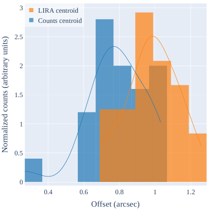
Figure 2: Histograms and corresponding kernel density curves of offsets measured using our method (orange) and using dmstat directly on the counts-image (blue).

3.2 A New X-ray Jet and Two Non-detections

For all cases, we verified that the chosen ROI contained statistically significant emission from the jet before measuring an offset. All the ROIs were consistent with previously reported detections of X-ray emission except in 3C 327.1 (p-value$\leq$0.08) and PKS 1402+044 (p-value$\leq$0.04). We could not confirm the presence of any significant X-ray emission from those two sources. The contours of the Chandra X-ray image of 3C 327.1, initially presented in Figure 18 of Massaro et al. (2013), suggested a jet-like structure that aligned with the radio jet. However, we observed a similar jet-like structure in a few of its baseline replicates, and our analysis with LIRA also did not indicate any significant X-ray emission from the jet.

We have detected new jet-linked emission from 3C 418 (see Fig. 3). This source shows a 3${}^{\prime\prime}$ knotty jet in the radio with multiple bends. The jet makes a 70° projected bend to the northwest at knot A and then makes another 60° projected bend to the northeast at knot B. Although its Chandra observation was first published in Jimenez-Gallardo et al. (2020), as the jet was within the PSF of the core, no jet detection was indicated. Our analysis using LIRA revealed a significant X-ray emission in an ROI constructed around knot B. We did not find evidence for X-ray emission from knots A and C. Interestingly, the centroid of the X-ray emission in knot B lies on the outer edge of the jet. This morphology suggests the jet itself may not be producing the observed X-ray emission. It may instead be originating from a jet-deflecting stationary obstacle (e.g., a dense gas cloud) that gets shock-heated by the jet (e.g., Worrall et al., 2016). Finally, in any of our sources, we found no significant emission from the core region that exceeded emission from a single point source (e.g., from an unresolved jet).

Figure 3: Results for the analysis for 3C 418, a quasar. With the VLA 8.4 GHz radio contours overlaid in the top panel–(a) The Chandra observation, binned by a factor of 0.5. (b) The average added component where the Red X marks the centroid of the added component within each ROI (dashed-green). (c)-(e) The posterior distributions of $\xi$ (fraction of the total emission in the added component) in each ROI for the observed image (shaded blue), 50 simulated images of the baseline model (gray) and their average (gray shaded area with a dashed-black curve). The radio contours are given by 2, 4, 8, 15 mJy/beam.

Table 3: Results for the offset analysis

Name	Component	Regiona	Offset			Counts	Optical/IRd	Spectral typee	p-value
		arcsecond${}^{2}$	″	Typeb	kpcc
3C 17	S10.8	e(0.65×0.70)	0.18	Xf	0.66	2	N	-	0.009
PKS 1311-270	B	c(0.6×0.6)	0.25	Xf	2.11	8	N	MSC (3)	0.005
3C 275.1	A	e(0.45×0.7)	0.65	Xf	4.16	19	N	MSC (3)	0.005
3C334	B	e(0.7×0.5)	0.22	Xf	1.46	14	N	MSC (3)	0.005
3C 17	S11.3	c(0.7×0.7)	0.15	Xf+Bnd	0.55	5	Y (a)	Amb (2)	0.005
0529+075	B	e(0.5×0.7)	0.56	Xf+Bnd	4.7	8	-	-	0.005
3C 179	D	c(0.5×0.5)	0.16	Xf+Bnd	1.23	4	N	MSC (3)	0.007
TXS 0833+585	B	c(0.4×0.6)	0.18	Xf+Bnd	1.54	8	-	-	0.005
PKS 1046-409	C	e(0.68×1.0)	0.54	Xf+Bnd	3.66	6	-	-	0.009
3C 280.1	D	e(0.85×0.5)	0.54	Xf+Bnd	4.65	5	N	MSC (3)	0.005
3C 6.1	NHS	c(1.25×1.25)	0.19	Xf	1.49	14	N	MSC (1)	0.005
3C 179	HS	c(0.6×0.6)	0.3	Xf	2.31	11	N	MSC (4)	0.005
4C+55.17	HS	e(0.4×0.6)	0.23	Xf	1.84	9	N	MSC (5)	0.006
PKS 1311-270	HS	e(0.57×0.90)	0.24	Xf	2.02	13	N	MSC (3)	0.005
PKS 2123-463	HS	c(0.97×0.97)	0.89	Xf	7.62	7	-	-	0.006
3C 6.1	SHS	c(0.8×0.8)	0.25	Xf+Bnd	1.96	4	N	MSC (1)	0.007
Centaurus B	A	c(1.0×1.0)	0.57	Rf	0.15	8	-	-	0.005
PKS 2123-463	A	c(0.6×0.6)	0.35	Rf	3	10	-	-	0.009
4C+11.45	C	e(0.44×0.55)	0.19	Rf+Bnd	1.61	8	N	MSC (3)	0.005
3C 17	S3.7	c(0.5×0.5)	0.12	(T) Xf	0.44	13	Y (a)	Amb (2)	0.005
3C133	B	c(0.7×0.7)	0.09	(T) Xf	0.03	8	Y (b)	MSC (3)	0.005
B3 1428+422	A	c(1.0×1.0)	0.09	(T) Xf	0.6	7	N	MSC (6)	0.005
4C+55.17	A	c(0.4×0.4)	0.07	(T) Xf	0.56	19	-	-	0.005
3C334	H	e(1.0×0.7)	0.12	(T) Xf+Bnd	0.8	8	N	MSC (3)	0.005
TXS 0833+585	A	c(0.6×0.6)	0.07	(T) Rf	0.6	11	-	-	0.006
3C213.1	NHS	c(0.65×0.56)	0.04	Co-s	0.133	3	Y (d)	MSC (3)	0.006
4C+25.21	HS	e(0.75×0.36)	0.02	Co-s	0.65	4	Y	MSC(3)	0.005
3C 220.2	SHS	e(0.42×0.35)	0.08	Unclear	0.68	3	Y (c)	MSC (2)	0.008
Potential high-redshift IC/CMB jets
4C+25.21	A	e (0.5×0.6)	-	-	-	7	-	-	0.007
PKS 2123-463	Jet	e(1.1×0.5)	-	-	-	5	-	-	0.009
Non-detections
PKS 1402+041	A	e(1.2×0.65)	-	-	-	14	-	-	0.04
PKS 1402+041	HS	c(0.6×0.6)	-	-	-	0	-	-	0.5
3C 327.1	A	r(3.3×1.6)	-	-	-	14	-	-	0.08
3C 327.1	B	e(0.75×0.5)	-	-	-	2	-	-	0.13
New detection
3C 418	A	c(0.4×0.4)	-	-	-	141	-	-	0.25
3C 418	B	c(0.5×0.5)	-	-	-	48	-	-	0.06
3C 418	C	c(0.5×0.5)	-	-	-	5	-	-	0.4

References. — Optical/IR detections: (a) Massaro et al. (2009). (b) Floyd et al. (2006). (c) This paper. (d) Floyd et al. (2006). Component spectral type: (1) Hardcastle et al. (2004). (2) Massaro et al. (2009). (3) This paper. (4) Sambruna et al. (2002). (5) Tavecchio et al. (2007). (6) Cheung et al. (2012).

3.3 Summary of all 22 sources

The main motivation for this study was to search for offsets in low-count Chandra observations that had not been analyzed previously. We have used the method outlined above to search for offsets in 22 low-count Chandra observations of jets. Although our main focus is on offsets in knots of MSC jets, we have also included hotspots and an FR-I source (Centaurus-B) for completeness, and in total 37 individual features were evaluated. The total number of counts in each feature ranged between 2 and 19 with 8.3$\pm$4.7 counts on average. Two knots in the inner jet in 3C 418 were excluded from this average as they were within the psf of the core with a large number of counts.

To claim an offset, we require the displacement between radio and X-ray position to be $>$0.15${}^{\prime\prime}$ given our (conservative) estimate of the registration error between radio and X-ray images and the X-ray positions which are both $\approx 0.05\arcsec$. With this requirement we have found clear offsets in 14 of the 22 jets analyzed, or 19 out of 28 features. Six sources each with one feature have a tentative or possible offset (0.05-0.15${}^{\prime\prime}$), and there is no evidence of offsets in one source ($<$0.05${}^{\prime\prime}$ separation). Of the clearly detected offsets, 16 are “X-ray first” type and 3 are “radio-first”. Of the tentative cases, 5 out of 6 are “X-ray first” type and one is “radio-first”.

The radio and X-ray observations in this study are not simultaneous (time baselines range from 0 to 24 years). Nevertheless we assume a negligible change in jet structure between radio and X-ray observations. Large-scale structural changes in the jet may be caused, for example, by kpc scale proper motions (e.g., Meyer et al., 2017; Snios et al., 2019) or changes in the jet orientation. However for proper motions to produce the observed offsets would require superluminal apparent motions on kpc scales with speeds of hundreds to thousands of times the speed of light, which is clearly unreasonable. Changes in the jet orientation, for example, by precession, will not affect our results as they happen on much larger time scales (e.g., Krause et al., 2019).

3.4 Optical/IR data and Spectral Analysis

To understand the spectral nature of the analyzed components, we also analyzed their corresponding HST data. Figures 26-35 display HST images overlaid with their respective radio contours. Components of four sources have detections at optical/IR wavelengths. Three are previously known, and we have newly identified IR emission from the southern hotspot of 3C 220.2. Furthermore, except in 3C 17, the rest of the HST detections are hotspots.

We fit a double-powerlaw phenomenological model (Uchiyama et al., 2006) to generate spectral energy distributions (SED). Where necessary, we used upper limits on the optical/IR fluxes for undetected components. For sources where HST data was available, except in the case of 3C 17, all the components required a second spectral component to explain the X-ray emission (see Table 3.2). For 3C 17, the existing signal to noise ratio (SNR) of the UV data does not permit differentiating between one or two spectral components (Massaro et al., 2009). The right panels of figures 26-35 show the SEDs whenever a fit was made.

3.5 Notes on Individual Sources

Here we give details on each of the 22 jets analyzed. Each source has a corresponding figure showing our analysis results, analogous to Figure 3 for 3C 418. In particular, except for 3C 6.1, we show in panel (a) the sub-pixel Chandra image of the jet, with radio contours overlaid in cyan. The dashed-green regions indicate the regions used to test the significance of emission and measure an offset unless otherwise stated. Solid-green circles indicate the region used to extract the spectrum of the core. In panel (b), we show the average of 2000 MCMC images from LIRA, with radio contours overlaid in black. A yellow X indicates the centroid for each region that is measured on the average added component. The rest of the images show the posterior density of $\xi$ for each analyzed region. Because of the large size of 3C 6.1, we show a zoomed-in version of its hotspots in (c) followed by the plots of posterior densities. In what follows, unless otherwise stated, the offsets are values that are projected onto the plane of the sky.

Table 3.2 summarizes the results of our analysis, with the name of the source in column 1, name of the analyzed feature in column 2, size of the region in column 3, offset (arcseconds) in column 4, type of the offset in column 5, sky-projected offset (kpc) in column 6, optical/IR detection status in column 7, the spectral type of the component in column 8 and the p-value in column 9. In column 6, “Xf” and “Rf” denote that the X-ray peaks closer and farther away from the core by more than 0.15${}^{\prime\prime}$, respectively, compared to the radio. Tentative offsets (0.05${}^{\prime\prime}$-0.15${}^{\prime\prime}$) are indicated with (T). “Co-s” indicates a feature where the X-ray centroid and radio peak are within 0.05${}^{\prime\prime}$ of each other; “Bnd” indicates that the feature lies at an apparent bend in the jet.

Figure 4: Results for the analysis of 3C 6.1, an FR-II NLRG–with the VLA 8.4 GHz radio contours overlaid in the top panel–(a) The Chandra observation, binned by a factor of 0.5. (b) The average added component. (c) Same as (a) and (b) but zoomed in to NHS (top) and SHS (bottom) respectively. The Red X marks the centroid of the added component within each ROI (dashed-green). The X-rays peak closer to the core than the radio in NHS. The jet appears to make a 90 deg turn to the west before reaching SHS where the X-rays peak upstream of the radio . (d)-(e) The distributions of $\xi$ in each ROI for the observed image (shaded blue), 50 simulated images of the baseline model (gray) and their average (gray shaded area with a dashed-black curve). The radio contours are given by 1.5, 8, 15, 40 mJy/beam.

3C 6.1 (Fig. 4) – This is an FR-II NLRG source with two X-ray hotspots. We find offsets of 0.19${}^{\prime\prime}$ (1.46 kpc) in the northern hotspot (NHS) and 0.25${}^{\prime\prime}$ (1.66 kpc) in the southern hotspot (SHS) with X-rays lying upstream of the radio.

Figure 5: Same as in Fig. 3, for 3C 17, an FR-II BLRG.

3C 17 (Fig. LABEL:fig:results_3C17): This is an FR-II BLRG source. We adopt the knot names from Massaro et al. (2009). The X-ray centroid and radio peak lie within 0.15${}^{\prime\prime}$ of each other in knot S3.7. Knots S11.3 and S10.8 show Xf-type projected offsets of 0.15${}^{\prime\prime}$ (0.55 kpc) and 0.18${}^{\prime\prime}$ (0.6 kpc) respectively. The jet bending at S11.3 presumably produces a internal shock where a strong shock at the bend produces X-rays while a weaker shock downstream produces radio (e.g., Worrall & Birkinshaw, 2005). Madrid et al. (2018) suggest that a dense intracluster medium might be responsible for bending the jet.

Figure 6: Same as in Fig. 3, with the VLA 4.8 GHz radio contours overlaid, for 3C 133, a HERG. The radio contours are given by 2, 4, 8, 10, 20, 40, 80 mJy/beam.

3C 133 (Fig. 6): This is an FR-II HERG source. The X-ray centroid in Knot A, which lies at a 90° projected apparent bend, lies within in 0.15${}^{\prime\prime}$ of its radio peak. Despite the X-ray emission from the knots in the inner-jet, we excluded them from the offset analysis as their separation was less than two ASCI-S pixels.

Figure 7: Same as in Fig. 3, with the VLA 4.8 GHz radio contours overlaid,, for 0529+075, a highly-superluminal CDQ. The radio contours are given by 1, 2, 3, 4, 8, 20, 100, 1000 mJy/beam.

0529+075 (Fig. 7): This is a core-dominated quasar. The inner jet makes a sharp apparent bend to the south and later turns to the southeast at knot B where it shows an Xf-offset of 0.56${}^{\prime\prime}$ (4.7 kpc).

Figure 8: Same as in Fig. 3, with the VLA 4.8 GHz radio contours overlaid,, for 3C 179, an LDQ. The radio contours are given by 0.3, 2, 4, 8 mJy/beam.

3C 179 (Fig. 8): This is a lobe-dominated quasar. The jet branches out into two directions–northwest and southwest–at knot D, where the X-ray centroid lies upstream of the radio peak by 0.16${}^{\prime\prime}$ (1.23 kpc). The northwestern branch terminates in a hotspot (HS) while the southwestern one diffuses away. Akujor (1992) suggest that a dense inter-galactic medium at D may be responsible for this splashing. The hotspot also shows an Xf-offset of 0.3${}^{\prime\prime}$ (2.31 kpc).

Figure 9: Same as in Fig. 3, for 4C+25.21, a high redshift quasar. The radio contours are given by 0.5, 2, 4, 8, 20 mJy/beam.

4C+25.21 (Fig. 9): This is a high-redshift quasar (z=2.68). The X-ray centroid lies within 0.15${}^{\prime\prime}$  of the radio peak in the hotspot. We also detect significant X-ray emission along a putative direction of the jet between the inner jet and the hotspot. This morphology suggests that IC/CMB presumably produces these X-rays (see section 4.4 for details).

Figure 10: Same as in Fig. 3, with the VLA 4.8 GHz radio contours overlaid, for TXS 0833+585, a high-redshift quasar. The radio contours are given by 0.34, 0.5, 2, 20, 200 mJy/beam.

TXS 0833+585 (Fig. 10): This is a hight redshift quasar (z=2.1). The X-ray centroid and the radio peak approximately coincide in knot A. In contrast, it lies upstream of the radio in knot B where the jet makes a 90° projected turn to the south. The flux ratio increases with distance from the core and may indicate that IC/CMB dominates the X-ray emission mechanism (see section 4.4 for details).

Figure 11: Same as in Fig. 3, for 3C 213.1, an LERG. The radio contours are given by 0.5, 2, 8, 40 mJy/beam.

3C 213.1 (Fig. 11): This an FR-II source. NHS is detected in radio, optical and X-rays. The X-ray centroid in NHS is within 0.05${}^{\prime\prime}$ (0.17 kpc) of the radio peak.

Figure 12: Same as in Fig. 3, for 3C 220.2, a quasar. The radio contours are given by 0.5, 2, 5, 20, 80 mJy/beam.

3C 220.2 (Fig. 12): This is a quasar. The X-ray centroid in SHS is within 0.15${}^{\prime\prime}$ (1.28 kpc) of its radio peak. However, unlike most of analyzed jet-features, the position angle of the tentative offset lies perpendicular to the putative direction of the jet. This morphology suggests that hot gases on kpc-scales may be emitting the X-rays rather than the hotspot itself.

Figure 13: Same as in Fig. 3, for 4C+55.17, a quasar/FSRQ. The radio contours are given by 2, 4, 8, 40, 100, 1000 mJy/beam.

4C+55.17 (Fig. 13): The classification for this source is ambiguous. It was initially classified as a quasar while McConville et al. (2011) suggest that it is a CSO. The X-ray centroid in knot A lies within 0.15${}^{\prime\prime}$ (0.14 kpc) of its radio peak. On the other hand, the hotspot (HS) shows an Xf-offset of 0.23${}^{\prime\prime}$ (1.84 kpc).

Figure 14: Same as in Fig. 3, with the ATCA 19 GHz radio contours overlaid, for PKS 1046-409, a CDQ. The radio contours are given by 1, 2, 4, 8, 100, 200 mJy/beam.

PKS 1046-409 (Fig. 14): This is a core-dominated quasar. The jet makes a projected 20° bend to the south at knot C, where the X-ray centroid lies upstream of the radio peak by 0.54${}^{\prime\prime}$ (4.65 kpc).

Figure 15: Same as in Fig. 3, with the VLA 4.8 GHz radio contours overlaid, for 3C 275.1, an LDQ. The radio contours are given by 0.5, 1, 2, 5, 70 mJy/beam.

3C 275.1 (Fig. 15): This is a lobe-dominated quasar. We find that knot A shows an Xf-offset offset of 0.65${}^{\prime\prime}$ (4.16 kpc).

Figure 16: Same as in Fig. 3, with the VLA 4.8 GHz radio contours overlaid, for 3C 280.1, an LDQ. The radio contours are given by 1, 4, 8, 20 mJy/beam.

3C 280.1 (Fig. 16): This is a lobe-dominated quasar. The jet makes a 30° bend to the south at knot D. This knot shows an Xf-offset of 0.54${}^{\prime\prime}$ (4.65 kpc). A bend in the jet at knot D may produce an internal shock and the onset of the bend could create a strong-shock which can produce X-rays while a weaker shock downstream can produce radio (e.g., Worrall & Birkinshaw, 2005).

Figure 17: Same as in Fig. 3, for PKS 1311-270, a high-redshift quasar. The radio contours are given by 0.5, 4, 10, 20 mJy/beam.

PKS 1311-270 (Fig. 17): This is a high-redshift quasar (z=2.19). Knot B shows an Xf-offset of 0.25${}^{\prime\prime}$ (2.11 kpc). The scenario is slightly complicated in the case of HS. The radio jet makes a 35° projected turn to the northeast before reaching HS. Although the X-ray centroid lies closer to the core than its radio peak [by 0.24${}^{\prime\prime}$ (2.02 kpc)], the offset is inconsistent with the direction of the jet. It is possible that the jet first turns towards the X-ray centroid before reaching the radio hotspot and projection effects create such an appearance. Alternatively, a large-scale hot and diffuse gas may be emitting the X-rays near HS.

Figure 18: Same as in Fig. 3, for 4C+11.45, a quasar.The radio contours are given by 0.3, 4, 20, 50, 80 mJy/beam.

4C+11.45 (Fig. 18): This is a quasar. The jet makes a 50° projected bend to the southeast at knot C, where the the X-ray centroid lies downstream of the radio peak by 0.19${}^{\prime\prime}$ (1.61 kpc).

Figure 19: Same as in Fig. 3, with the ATCA 8.6 GHz radio contours overlaid, for Centaurus B, an FR-I RG. The radio contours are given by 8, 15, 20, 100, 1000 mJy/beam.

Centaurus B (Fig. 19): This is an FR-I source. Knot A shows an Rf-type offset of 0.57${}^{\prime\prime}$ (0.15 kpc). Such an offset is rarely observed in jets with an FR-I type morphology.

Figure 20: Same as in Fig. 3, with the VLA 1.4 GHz radio contours overlaid, for B3 1428+422, a high-redshift quasar. The radio contours are given by 0.2, 1, 10, 100 mJy/beam.

B3 1428+422 (Fig. 20): This is one of the highest redshift (z=4.7) X-ray jet known to date. We find that the X-ray centroid in its jet-related feature, A, lies within 0.15${}^{\prime\prime}$ (1 kpc) of its radio peak.

Figure 21: Same as in Fig. 3, with the VLA 4.8 GHz radio contours overlaid, for 3C 334, a quasar. The radio contours are given by 0.15, 0.4, 0.7, 5, 10, 40 mJy/beam.

3C 334 (Fig. 21): This is a quasar. Knot B shows an Xf-offset of 0.22${}^{\prime\prime}$ (1.46 kpc). In contrast, the X-ray centroid in H, where the jet makes a 90° apparent bend to the northeast, lies within 0.15${}^{\prime\prime}$ (1 kpc) of its radio peak.

3C 418 (Fig. 3): This is a quasar. We newly detect jet-linked X-ray emission from knot B using LIRA. See section 3.2 for details.

Figure 22: Same as in Fig. 3, for PKS 2123-463, with the ATCA 18 GHz radio contours overlaid, a high redshift quasar. The radio contours are given by 1.3, 2, 4 mJy/beam.

PKS 2123-463 (Fig. 22): This is a core-dominated quasar. Knot A shows an Rf-type offset of 0.35${}^{\prime\prime}$ (3 kpc) while the hotspot shows an Xf-offset of 0.89${}^{\prime\prime}$ (7.62 kpc). We also detect significant X-ray emission along the putative direction of the jet between knot A and the hotspot, which, similar to 4C+25.21, suggests that IC/CMB presumably produces these X-rays (see section 4.4 for details).

Figure 23: Same as in Fig. 3, with the VLA 4.8 GHz radio contours overlaid, for PKS 1402+044, a high-redshift quasar. The radio contours are given by 0.8, 1.5, 8, 40 mJy/beam.

PKS 1402+044 (Fig. 23): This is a high-redshift quasar (z=3.2). We could not confirm (p-value$\leq$0.04) any significant X-ray emission from the jet of this source, unlike the previous authors in Schwartz et al. (2019).

Figure 24: Same as in Fig. 3, for 3C 327.1, a HERG. We did not measure the offset as there was no statistically significant emission from the chosen ROIs. The radio contours are given by 0.5, 2, 10, 25, 40 mJy/beam.

3C 327.1 (Fig. 24): This is an FR-II source. Similar to PKS 1402+044, contrary to the previous claim in Massaro et al. (2013), we could not confirm (p-value$\leq$0.15) the presence of any significant X-ray emission from its jet.

4 Discussion

4.1 Offset Statistics

In the majority (10 out of 13) of the clearly detected ($>$0.15${}^{\prime\prime}$ separation) knot offsets, the X-ray centroid lies upstream of its corresponding radio peak (denoted as Xf or X-ray-first). Xf-offsets are also the majority (5 out of 6) amongst the tentative cases and are also the predominant type reported in the literature (e.g., Sambruna et al., 2004; Worrall & Birkinshaw, 2005; Siemiginowska et al., 2007; Clautice et al., 2016; Worrall et al., 2016; Harris et al., 2017; Marchenko et al., 2017). These offsets contradict an observational requirement of the commonly adopted IC/CMB models which expects the X-rays to either be coincident or extend beyond the radio (Harris & Krawczynski, 2007; Worrall, 2009).

In only three sources, Centaurus B, PKS 2123-463 and 4C+11.45, the X-ray centroid lies downstream of its radio peak (denoted as Rf or Radio-first), which are consistent with the IC/CMB interpretation. Marscher & Jorstad (2011) have previously noted such an offset in the jet of OJ 287, a BL Lac object. Recently, Meyer et al. (2019) have concluded that IC/CMB is its dominant X-ray emission mechanism. They measured the $\gamma$-ray flux from the jet and showed that it equals the level expected from the observed X-ray emission under IC/CMB (see Georganopoulos et al., 2006). For Centaurus B and PKS 2123-463, lack of observations in the optical prevents one from using the gamma-rays to test for steady IC/CMB from these source since the IR/optical is generally required to predict the gamma-ray flux level. However, the FR-II type morphology of PKS 2123-463 suggests that this is presumably an MSC-type jet and its Rf-offset may therefore indicate that IC/CMB is the dominant mechanism. We have also found significant extended X-ray emission between its inner knot and hotspot without any associated radio emission. This morphology combined with its high redshift also suggests that IC/CMB dominates X-ray emission from the jet (see section 4.5 for details). In the case of 4C+11.45, the X-rays may instead be produced by a dense gas that deflects the jet while also getting shock heated by it (see Fig. 18, where the extended nature of the jet-region emission is evident). Optical maps of 4C+11.45 presented in Lehnert et al. (1999) and Heckman et al. (1991) show large Ly$\alpha$ clouds around this offset and support the deflection scenario.

Our sample contains five highly-superluminal sources with apparent jet speeds greater than 3.36, which are of interest because the high apparent jet speeds imply that the parsec-scale jet is at a small angle to the line-of-sight. In such sources, presuming no major change in orientation between the parsec and kpc scales, real offsets between the location of radio and X-ray emission might be more difficult to distinguish due to the extreme foreshortening of the jet. Of these five, we could not confirm the presence of X-ray emission from the jet in one source, PKS 1402+044. In the remaining sources we do detect an offset. Interestingly, three of them appear at an apparent bend in the jet (indicated with “+Bnd” in column 5 of Table 3.2). In jets which are overall well-aligned, small deflections (changes in jet angle) can appear very extreme due to the effects of projection. This may explain sources like TXS 0833+585 [$\beta_{app}=14.16$ Britzen et al. (2008); Keenan et al. (2020); Fig. 10], where the inner-most knot A in shows only a small offset (0.07${}^{\prime\prime}$) while the outer knot B, which lies at an apparent bend, shows an Xf-offset (0.18${}^{\prime\prime}$). We can interpret these observations as a combined result of projection effects and limited instrumental resolution. The observed $\beta_{app}$ limits the viewing angle of the pc-scale jet to at most $\sim$8°. Hence, for a small pc-to-kpc scale deflection, projection effects would shorten any offset in knot A by a factor of seven, and we may not resolve it. If both the knots contain offsets of similar magnitudes, then an offset in knot B suggests that the jet is more misaligned at this bend, thereby making the offset more apparent. Two other scenarios are also possible: (i) The offset in knot B is relatively higher (see section 4.3), which may only require a small deflection in the jet. (ii) Knot A may be intrinsically different from knot B and actually exhibit no offset. Distinguishing between these scenarios would require next-generation X-ray observatories with much higher resolution.

Figure 25: Offsets and flux ratios plotted against various parameters. (a) Normalized offset is plotted against normalized distance from core for selected jets. (b) Same as (a) but with de-projected values. In (a) and (b) dot indicates a bent jet and the error bars are fixed at 0.1${}^{\prime\prime}$; Triangles denote knots with tentative offsets and are fixed at 0.15${}^{\prime\prime}$(upper limit). See the text for details on the angles used and associated uncertainties. (c) Flux ratio is plotted against normalized distance from core; squares indicate hotspots and circles knots, and lines indicate selected jets. Stars indicate features with only one X-ray feature in the jet. (d) Flux ratio is plotted against the inclination angle of the jet.

4.2 De-projecting the offsets

Table 3.2 provides lower-limits for the true offsets that are also projected onto the plane of the sky. Understanding the nature of these offsets would first require de-projecting them, which in turn requires the alignment angle of the jet. Although a few methods exist in the literature to estimate the alignment angle, for instance, from the ratio of core to lobe luminosities (e.g., Drouart et al., 2012; Marin & Antonucci, 2016), they only apply for specific redshift ranges and have large uncertainties for closely aligned sources. Because our sample covers a wide redshift range and contains superluminal sources, to start, we assigned representative upper-limits to the orientation angles based on their class. Adopting the mean angle estimates from the unification scheme proposed in Urry & Padovani (1995), we assigned an angle of 15°  to the CDQ class, 30° for LDQ, 60° for BLRG and 90° for NLRG. The choice of 60°  for BLRG type sources is consistent with the recent estimates of the half-opening angle of the torus (Sazonov et al., 2015; Marin & Antonucci, 2016). When no sub-classification was available for a quasar, we assigned it a value of 40° . For jets with apparent bends larger than 20°, we assumed an additional 15°  increment. Assuming the maximum possible non-disruptive bend in a relativistic jet is $\approx 49$°  (Mendoza & Longair, 2002), even small orientation effects are sufficient to produce large projected bends. Hence this increment may over-estimate the angle for closely aligned jets (e.g., quasars).

4.3 De-projected offset versus distance from core

We can also examine if and how the offsets are related to other properties of the jet. In a detailed study on 3C 353, a nearby FR-II jet, (Kataoka et al., 2008) have found that the offsets in knots and hotspots increased with distance from the core. They also argued that 3C 353 is a representative FR-II source, and one can expect such a progression in other similar X-ray jets. We searched for similar trends in our sample by selecting jets with at least two X-ray components on one side of the jet. Besides using the de-projected values, we also normalized offsets and distances by dividing them with the total length of the jet (measured from core to hotspot, along the jet). The normalized distance is independent of the alignment angle of the jet. For bent jets, this normalization would only modify the rate of increase would and not the increasing trend itself.

Figure 25a shows normalized offset plotted against normalized distance from core and Figure 25b shows its de-projected version. We also added data from Kataoka et al. (2008) to both the figures for comparison. Triangles denote knots with tentative Xf-offsets and are fixed at 0.15${}^{\prime\prime}$(upperlimit). Dotted markers indicate a bent jet. In three of the six sources, the offsets increase with distance from core, consistent with 3C 353. The offsets in two of the remaining sources stay approximately constant. Only in 3C 334, a knot in the inner jet shows an Xf-offset while a knot at a bend that disrupts the jet shows no offset. Given the errors in measuring the offsets, further studies on a larger sample are necessary to establish the presence or absence of any trend between offsets and distance from core.

4.4 X-ray-to-radio Flux ratio

We measured the X-ray-to-radio flux ratio ($\nu_{X}F_{X}/\nu_{R}F_{R}$; flux ratio, hereafter) by evaluating the X-ray flux at 1 keV. We chose 4.8 GHz for the radio based on its availability for most sources, except in PKS 1046-409 and 3C 179, where we used the fluxes at 19 GHz and 8.4 GHz, respectively. The flux ratio is known to systematically decrease along the jet in many cases (e.g., Sambruna et al., 2004; Siemiginowska et al., 2007; Kataoka et al., 2008). It is possible that, within the IC/CMB model, the jet decelerates on kiloparsec-megaparsec scales via mass entrainment (Georganopoulos & Kazanas, 2004) and produces a declining flux ratio. However, Hardcastle (2006) found no significant trend for decelerating jets and noted that the cold matter required for entrainment is sometimes unreasonably high. Kataoka et al. (2008) have speculated that, within the synchrotron model, changing plasma conditions along the jet instead causes a gradual decline in the X-ray emission.

In our sample, we also notice a slight trend where the flux ratio tends to decrease with normalized distance from core (Fig. 25c), except in TXS 0833+585, where the opposite happens (see section 4.5 for details). Correlation tests revealed a significant correlation between the two variables (for the entire sample), with Pearson’s $R$=-0.47 (p-value=0.018) and Spearman’s $\rho$=-0.48 (p-value=0.015). Although this trend is consistent with IC/CMB in a decelerating jet, it does not necessarily imply that IC/CMB dominates X-ray emissions from all the jets. We might instead, for instance, speculate that a faster spine up-scatters radio emission from a slower enclosing-sheath to X-ray wavelengths, and when combined with a decelerating jet, can also reproduce the observed trend. Furthermore, the IC/CMB model expects the flux ratio to decrease with increasing angle because the X-rays will be de-beamed faster than the radio. However, we did not find any significant evidence for such a trend (Fig. 25d) in our small sample, suggesting a synchrotron origin for the X-rays. This result is consistent with the findings in Massaro et al. (2011) where the authors reported no difference between the flux-ratio distributions of knots in quasars (smaller alignment angles) and FR-IIs (larger alignment angles). We also tested for a correlation between offsets and flux ratio but found none.

4.5 High redshift jets and IC/CMB

While it seems increasingly unlikely that lower-redshift MSC jets have X-rays dominated by the IC/CMB process, this is not true of high-redshift jets, especially cases where X-rays have been observed with little to no corresponding radio emission (e.g., Yuan et al., 2003; Cheung et al., 2012; Simionescu et al., 2016; McKeough et al., 2016; Worrall et al., 2020). In light of this, we identified three high-redshift sources in our sample for further scrutiny. In TXS 0833+588 (z=2.1), the flux ratio increases along the jet, contrary to the general decreasing trend. Moreover, of the two knots in this jet, the knot farther away from the core appears at an apparent bend. Because under the IC/CMB model, the X-rays are more beamed than the radio, stronger brightening in the X-rays at this point could be attributed to a small decrease in orientation angle at the bend. However, IC/CMB requires unreasonable kpc scale speeds to produce the observed X-rays in this knot. (2018ApJ...856...66M). Interestingly, the Xf-offset in this knot also argues against IC/CMB while the Rf-offset (tentative) in the inner knot is consistent with it. Hence, there may be multiple X-ray emission processes in the outer knot (e.g., an intrinsically brighter component), which, however, cannot be confirmed with the available data.

In the two other high-redshift jets, PKS 2123-463 (z=1.67; Fig. 22) and 4C+25.21 (z=2.69; Fig. 9), it appears that X-ray emission may be present along portions of the jet between the core and the hotspot that lacks significant radio emission. Simionescu et al. (2016) have observed a similar morphology where the X-ray jet in B3 0727+409 (z=2.5) lacked a radio counterpart. They found that the existing data favours IC/CMB over the synchrotron interpretation. Therefore, although we only selected regions with well-defined radio emission to detect offsets, for PKS 2123-463 and 4C+25.21, we also analyzed regions without any radio emission and confirmed the presence of X-ray emission at a high significance. In both cases the X-ray emission in these regions appears to extend past the radio, a general characteristic of the IC/CMB interpretation (Harris & Krawczynski, 2007; Worrall, 2009). However, the situation is slightly ambiguous in the case of 4C+25.21 as the detected X-ray emission not only lies downstream of a bright inner jet but also upstream of a much fainter radio peak near the hotspot. These results further support the idea of a new class of high-redshift X-ray jets that lack radio emission (Simionescu et al., 2016). However, it should be noted that such a morphology can be interpreted in an alternate way: instead of the jet, the lobes may also emit the observed X-rays via IC/CMB (e.g., Erlund et al., 2008; Wu et al., 2017). In this case the low-frequency radio spectral index of the lobes and the X-ray emission are expected to match. However, it is impossible to distinguish between the two scenarios with the available data and deeper radio and X-ray observations are necessary.

5 Summary

We have demonstrated a method to detect X-ray-to-radio offsets from low-count X-ray images using a powerful statistical tool called LIRA (Esch et al., 2004; Stein et al., 2015). Using a deep observation of PKS 0605–08, we showed that our method not only can accurately detect an offset under the low-count regime but also can provide an associated error.. Our analysis of 37 features in 22 jets detected by Chandra in the low-count (<20) regime has revealed a significant number of ‘X-ray first’ offsets – 16 are clear detections ($>0.15^{\prime\prime}$ separation) while 5 are tenative ($0.05-0.15^{\prime\prime}$ separation). These greatly outnumber the number of Radio-first detections (3) or tentative detections (1), and only one jet/feature appears completely co-spatial. We adopted a representative orientation scheme for the jets to de-project the offsets. In most of our sources, the offsets tend to increase with distance from core while the flux ratio decreases. We also identified three potential high-redshift jets where the X-ray emission may be dominated by the IC/CMB process. In two of these, we find evidence of X-ray emission without corresponding radio emission; in the third one, the flux ratio increases with distance from the core. Future work with a larger sample of X-ray detected jets will be needed to confirm the trends found here.

Appendix A Optical/IR images and SEDs

Figure 26: Results for the optical and spectral analysis of 3C 6.1. (a) The HST Wide Field Planeraty Camera 2 (WFCP2) visible image at 5.5 $\times 10^{14}$ GHz (5439 Å) with the VLA 8.6 GHz radio contours overlaid. The left and right panes show NHS and SHS, respectively. Both the hotspots are not detected at this wavelength. (b) The broadband SEDs of NHS and SHS which indicate that X-rays require a second spectral component.

Figure 27: The HST Space Telescope Imaging Spectrograph (STIS) visible image at 4.16 $\times$ 10${}^{14}$ Hz (7216 Å) of 3C17 overlaid with the VLA 4.86 GHz radio contours. Knots S3.7 and S11.3 are detected in the optical.

Figure 28: Results for the optical and spectral analysis of 3C 133. (a) The HST Near Infrared Camera and Multi-Object Spectrometer-2 (NICMOS-2) infrared image (IR) at 1.87 $\times 10^{14}$ GHz (16030 Å) with the VLA 4.86 GHz radio contours overlaid. (b) The broadband SED of knot B which indicates that the X-ray emission requires a separate spectral component.

Figure 29: Results for the optical and spectral analysis of 3C 213.1. (a)The HST NICMOS-2 infrared image at 1.87 $\times 10^{14}$ GHz (16030 Å) with the VLA 8.6 GHz radio contours overlaid. (b) The broadband SED of NHS which indicates that X-rays require a second spectral component.

Figure 30: Results for the optical and spectral analysis of 3C 220.2. (a) The HST Wide Field Camera-3 (WFC3) IR image at 2.15 $\times 10^{14}$ GHz (13922 Å) with the VLA 8.4 GHz radio contours overlaid. (b) The broadband SED of SHS which indicates that the X-rays require a separate spectral component.

Figure 31: Results for the optical and spectral analysis of 3C 275.1. (a) The HST WFPC2 visible image at 4.46 $\times 10^{14}$ GHz (6717 Å) with the 8.4 GHz radio contours overlaid. Knot A is not detected at this wavelength. (b) The broadband SED of knot A which indicates that X-rays requires a second sepctral component.

Figure 32: Results for the optical and spectral analysis of 3C 280.1. (a) The HST WFPC3 IR at 2.15 $\times 10^{14}$ GHz (13922 Å) with the 4.8 GHz radio contours overlaid. Knot D is not detected at the IR wavelength. (b) The broadband SED of knot D where a two-component phenomenological fit was not possible. However, a single component is fit to the radio data which clearly cannot explain the observed X-ray emission.

Figure 33: Results for the optical and spectral analysis of PKS 1311-270. (a) The HST WFPC2 visible image at 4.46 $\times 10^{14}$ GHz (6717 Å) with the 8.4 GHz radio contours overlaid. Knot B and HS are not detected at this wavelength. (b) The broadband SEDs of B and HS which indicate that the X-ray emission from both the components requires a second spectral component.

Figure 34: Results for the optical and spectral analysis of 4C+11.45. (a) The HST WFPC2 visible image at 5.5 $\times 10^{14}$ GHz (5439 Å) with the VLA 8.4 GHz radio contours overlaid. Knot C is not detected at this wavelength. (b) The broadband SED of knot C which indicates that X-rays requires a second spectral component.

Figure 35: Results for the optical and spectral analysis of 3C 334. (a) The HST WFPC2 visible image at 5.5 $\times 10^{14}$ GHz (5439 Å) with the VLA 8.4 GHz radio contours overlaid. Knots B and H are not detected at this wavelength. (b) The broadband SEDs of knots B and H which indicates that X-rays from both the components requires a second spectral component.

Appendix B List of sources with low-count Chandra observations

Table 4: Summary of Chandra detected low-count X-ray jets

Namea	IAU Nameb	R.A. (J2000)c
	decl. (J2000)c	hh:mm:ss
	zd		Scalee
		Classf	Jet detectiong
			paper
Sources used for analysis
3C 6.1 (catalog )	0013+790	00:16:31.147	+79:16:49.88	0.8400		7.84		FR II (NLRG)	Hardcastle et al. (2004)
3C 17 (catalog )	0035-024	00:38:20.520	-02:07:40.72	0.2200		3.64		FR II (BLRG)	Massaro et al. (2009)
3C 133 (catalog )	0459+252	05:02:58.480	+25:16:25.11	0.2775		4.34		FR II (HERG)	Massaro et al. (2010)
0529+075 (catalog )‡	0529+075	05:32:38.998	+07:32:43.34	1.2540		8.40		CDQ	Hogan et al. (2011)
3C 179 (catalog )‡	0723+679	07:28:10.896	+67:48:47.03	0.8460		7.70		LDQ	Sambruna et al. (2004)
4C+25.21 (catalog )	0730+257	07:33:08.78	+25:36:25.02	2.6860		8.135		Q	McKeough et al. (2016)
TXS 0833+585 (catalog )‡	0833+585	08:37:22.409	+58:25:1.84	2.1010		8.53		Q	McKeough et al. (2016)
3C 213.1 (catalog )	0858+292	09:01:05.25	+29:01:46.90	0.1939		3.33		FR II (LERG)	Massaro et al. (2010)
3C 220.2 (catalog )	0927+362	09:30:33.473	+36:01:24.17	1.1574		8.47		Q	Stuardi et al. (2018)
4C +55.17 (catalog )	0954+556	09:57:38.184	+55:22:57.76	0.8996		8.01		Q/CSO	Tavecchio et al. (2007)
PKS 1046-409 (catalog )	1046-409	10:48:38.270	-41:14:00.11	0.6200		6.78		CDQ	Marshall et al. (2005)
3C 275.1 (catalog )	1241+266	12:43:57.649	+16:22:53.39	0.5550		6.40		LDQ	Crawford & Fabian (2003)
3C 280.1 (catalog )	1258+404	13:00:33.364	+40:09:07.28	1.6771		8.62		LDQ	Jimenez-Gallardo et al. (2020)
PKS 1311-270 (catalog )	1311-270	13:13:47.360	-27:16:49.27	2.1860		8.43		Q	McKeough et al. (2016)
4C+11.45 (catalog )	1318+113	13:21:18.835	+11:6:49.98	2.1792		8.48		Q	McKeough et al. (2016)
Centaurus B (catalog )	1343-601	13:46:48.990	-60:24:29.96	0.0130		0.26		FRI RG	Marshall et al. (2005)
PKS 1402+044 (catalog )*‡	1402+044	14:05:01.12	+04:15:35.82	3.2091		7.73		Q	Schwartz et al. (2019)
B3 1428+422 (catalog )	1428+422	14:30:23.741	+42:04:36.49	4.7150		6.61		Q	Cheung et al. (2012)
3C 327.1 (catalog )*	1602+014	16:04:45.320	+01:17:51.02	0.4620		6.02		FR II (HERG)	Massaro et al. (2013)
3C 334 (catalog )‡	1618+177	16:20:21.818	+17:36:2.95	0.5551		6.63		Q	Hardcastle et al. (2004)
3C 418 (catalog )‡	2037+511	20:38:37.042	+51:19:12.43	1.6860		8.61		Q	This work†
PKS 2123-463 (catalog )	2123-463	21:26:30.704	-46:05:47.90	1.6700		8.56		CDQ	Marshall et al. (2011)
Sources excluded from analysis
3C 13 (catalog )	0031+391	00:34:14.556	39:24:16.65	1.3510		8.63		FR II (HERG)	Wilkes et al. (2013)
3C 16 (catalog )	0035+130	00:37:44.573	+13:19:54.99	0.4050		5.567		FR II (HERG)	Massaro et al. (2013)
3C 19 (catalog )	0038+328	0:40:55.0440	+33:10:8.0200	0.4820		6.15		FR II (LERG)	Massaro et al. (2015)
3C 52 (catalog )	0145+532	01:48:28.977	+53:32:35.44	0.2900		4.47		FR II (HERG)	Massaro et al. (2010)
3C 41 (catalog )	0123+239	01:26:44.300	+33:13:11.00	0.7950		7.70		FR II (HERG)	Massaro et al. (2018)
3C 54 (catalog )	0152+435	01:55:30.162	+43:45:55.43	0.8270		7.81		FR II (HERG)	Massaro et al. (2018)
3C 61.1 (catalog )	0210+860	02:22:35.046	+86:19:06.17	0.1878		3.32		FR II (HERG)	Massaro et al. (2010)
3C 65 (catalog )	0220+397	02:23:43.191	+40:00:52.45	1.1760		8.49		FR II (HERG)	Wilkes et al. (2013)
3C 68.2 (catalog )	0231+313	02:34:23.856	+31:34:17.46	1.5750		8.69		FR II (HERG)	Wilkes et al. (2013)
0313-192 (catalog )	0313-192	03:15:52.100	-19:06:44.30	0.0670		1.27		FR I RG	Keel et al. (2006)
3C 129 (catalog )	0445+449	04:49:09.064	+45:00:39.40	0.0208		0.42		FR I RG	Harris et al. (2002)
3C 181 (catalog )	0725+147	07:28:10.305	14:37:36.24	1.3820		8.64		Q	Wilkes et al. (2013)
3C 189 (catalog )	0755+379	07:58:28.108	+37:47:11.80	0.0428		0.83		FR I RG	Worrall et al. (2001)
3C 191 (catalog )	0802+013	08:04:47.972	10:15:23.69	1.9560		8.60		Q	Erlund et al. (2006)
4C+05.34 (catalog )	0805+046	08:07:57.54	+04:32:34.53	2.8770		7.99		Q	McKeough et al. (2016)
3C 200 (catalog )	0824+294	08:27:25.397	+29:18:44.90	0.4580		5.99		FR II (LERG)	Hardcastle et al. (2004)
3C 210 (catalog )	0855+280	08:58:09.961	+27:50:51.57	1.1690		8.48		FR II (HERG)	Gilmour et al. (2009)
PKS 0903-573 (catalog )	0903-573	09:04:53.179	-57:35:05.80	0.6950		7.12		CDQ	Marshall et al. (2005)
4C+39.24 (catalog )	0905+399	09:08:16.900	+39:43:26.00	1.882		8.63		FR II (HERG)	Erlund et al. (2008)
3C 219 (catalog )	0917+458	09:21:08.626	+45:38:57.34	0.1740		2.90		FR II RG (HERG)	Comastri et al. (2003)
3C 225B (catalog )	0939+139	09:42:15.387	+13:45:50.52	0.5800		6.77		FR II (HERG)	Massaro et al. (2018)
3C 238 (catalog )	1008+066	10:11:00.379	+06:24:39.72	1.4050		8.65		FR II (HERG)	Stuardi et al. (2018)
3C 239 (catalog )	1008+467	10:11:45.284	+46:28:18.79	1.7810		8.60		FR II (HERG)	Jimenez-Gallardo et al. (2020)
3C 249 (catalog )	1059-009	11:02:03.774	-01:16:16.67	1.5540		8.61		LDQ	Jimenez-Gallardo et al. (2020)
3C 257 (catalog )	1120+057	11:23:09.391	+05:30:18.50	2.4740		8.25		FR II	Jimenez-Gallardo et al. (2020)
3C 268.1 (catalog )	1157+732	12:00:19.210	+73:0:45.70	0.9700		8.17		FR II (HERG)	Massaro et al. (2015)
3C 268.2 (catalog )	1158+318	12:00:59.110	+31:33:27.90	0.3620		5.21		FR II (HERG)	Massaro et al. (2012)
3C 280 (catalog )	1254+476	12:56:57.900	+47:20:19.90	0.9960		8.00		FR II (HERG)	Donahue et al. (2003)
3C 281 (catalog )	1305+069	13:07:53.929	+06:42:14.30	0.6020		6.70		LDQ	Crawford & Fabian (2003)
4C+65.15 (catalog )	1323+655	13:25:29.702	+65:15:13.293	1.6250		8.60		LDQ	Miller & Brandt (2009)
3C 293 (catalog )	1350+316	13:52:17.842	+31:26:46.50	0.0450		0.92		FR I (LERG)	Massaro et al. (2010)
3C 297 (catalog )	1414-037	14:17:23.999	-04:00:47.54	1.4061		8.65		Q	Stuardi et al. (2018)
3C 313 (catalog )	1508+080	15:11:00.010	+07:51:50.00	0.4610		6.01		FR II (HERG)	Massaro et al. (2013)
3C 322 (catalog )	1533+557	15:35:01.26	+55:36:52.33	1.6810		8.61		FR II	Jimenez-Gallardo et al. (2020)
3C 324 (catalog )	1547+215	15:49:48.900	+21:25:38.10	1.2063		8.40		FR II (HERG)	Hardcastle et al. (2004)
3C 326.1 (catalog )	1553+202	15:56:10.170	+20:04:20.73	1.8250		8.57		RG	Jimenez-Gallardo et al. (2020)
TXS 1607+183 (catalog )	1607+183	16:10:05.28	18:11:43.41	3.1180		7.80		Q	Schwartz et al. (2019)
3C 341 (catalog )	1626+738	16:28:4.050	+27:41:43.00	0.4480		5.91		FR II (HERG)	Massaro et al. (2013)
3C 349 (catalog )	1658+371	16:59:29.540	+47:02:44.10	0.2050		3.46		FR II (HERG)	Massaro et al. (2010)
3C 368 (catalog )	1802+110	18:05:06.454	+11:01:35.06	1.131		8.44		FR II (HERG)	Wilkes et al. (2013)
3C 402 (catalog )	1940+504	19:41:46.050	+50:35:48.40	0.0259		0.53		FR I	Massaro et al. (2012)
3C 436 (catalog )	2141+279	21:44:11.708	+28:10:19.030	0.2145		8.68		FR II (HERG)	Massaro et al. (2010)
3C 437 (catalog )	2145+151	21:47:25.106	+15:20:37.49	1.4800		8.68		FR II	Massaro et al. (2015)
PKS 2155-152 (catalog )‡	2155-152	21:58:06.282	-15:01:09.32	0.6720		7.02		CDQ	Hogan et al. (2011)
PKS 2255-282 (catalog )‡	2255-282	22:58:05.962	-27:58:21.30	0.9260		7.88		CDQ	Marshall et al. (2011)
3C 458 (catalog )	2310+050	23:12:54.408	+05:16:45.98	0.2890		4.46		FR II (HERG)	Massaro et al. (2012)
3C 470 (catalog )	2356+437	23:58:35.890	+44:4:45.55	1.653.		8.69		FR II	Hogan et al. (2011)

Note. — All the cosmological parameters are taken from NASA/IPAC Extragalctic Database(NED).

References

- Akujor (1992) Akujor, C. E. 1992, A&A, 259, L61
- Avila et al. (2015) Avila, R. J., Hack, W., Cara, M., et al. 2015, in Astronomical Society of the Pacific Conference Series, Vol. 495, Astronomical Data Analysis Software an Systems XXIV (ADASS XXIV), ed. A. R. Taylor & E. Rosolowsky, 281. https://arxiv.org/abs/1411.5605
- Bai & Lee (2003) Bai, J. M., & Lee, M. G. 2003, The Astrophysical Journal Letters, 585, L113
- Blandford & Königl (1979) Blandford, R., & Königl, A. 1979, The Astrophysical Journal, 232, 34
- Blandford et al. (2019) Blandford, R., Meier, D., & Readhead, A. 2019, Annual Review of Astronomy and Astrophysics, 57, 467
- Böttcher (2019) Böttcher, M. 2019, Galaxies, 7, 20, doi: 10.3390/galaxies7010020
- Breiding et al. (2017) Breiding, P., Meyer, E. T., Georganopoulos, M., et al. 2017, The Astrophysical Journal, 849, 95
- Bridle & Perley (1984) Bridle, A. H., & Perley, R. A. 1984, Annual review of astronomy and astrophysics, 22, 319
- Britzen et al. (2008) Britzen, S., Vermeulen, R., Campbell, R., et al. 2008, Astronomy & Astrophysics, 484, 119
- Celotti et al. (2001) Celotti, A., Ghisellini, G., & Chiaberge, M. 2001, Monthly Notices of the Royal Astronomical Society, 321, L1
- Cheung et al. (2012) Cheung, C. C., Stawarz, Ł., Siemiginowska, A., et al. 2012, ApJ, 756, L20, doi: 10.1088/2041-8205/756/1/L20
- Cheung et al. (2012) Cheung, C. C., Stawarz, Ł., Siemiginowska, A., et al. 2012, The Astrophysical Journal, 756, L20, doi: 10.1088/2041-8205/756/1/l20
- Clautice et al. (2016) Clautice, D., Perlman, E. S., Georganopoulos, M., et al. 2016, Astrophys. J., 826, 109, doi: 10.3847/0004-637X/826/2/109
- Comastri et al. (2003) Comastri, A., Brunetti, G., Dallacasa, D., et al. 2003, MNRAS, 340, L52, doi: 10.1046/j.1365-8711.2003.06561.x
- Crawford & Fabian (2003) Crawford, C., & Fabian, A. 2003, Monthly Notices of the Royal Astronomical Society, 339, 1163
- Croton et al. (2006) Croton, D. J., Springel, V., White, S. D., et al. 2006, Monthly Notices of the Royal Astronomical Society, 365, 11
- Davis et al. (2012) Davis, J. E., Bautz, M. W., Dewey, D., et al. 2012, in Society of Photo-Optical Instrumentation Engineers (SPIE) Conference Series, Vol. 8443, Proc. SPIE, 84431A, doi: 10.1117/12.926937
- Doe et al. (2007) Doe, S., Nguyen, D., Stawarz, C., et al. 2007, in Astronomical Society of the Pacific Conference Series, Vol. 376, Astronomical Data Analysis Software and Systems XVI, ed. R. A. Shaw, F. Hill, & D. J. Bell, 543
- Donahue et al. (2003) Donahue, M., Daly, R. A., & Horner, D. J. 2003, The Astrophysical Journal, 584, 643
- Drouart et al. (2012) Drouart, G., De Breuck, C., Vernet, J., et al. 2012, Astronomy & Astrophysics, 548, A45
- Erlund et al. (2006) Erlund, M. C., Fabian, A., Blundell, K. M., Celotti, A., & Crawford, C. 2006, Monthly Notices of the Royal Astronomical Society, 371, 29
- Erlund et al. (2008) Erlund, M. C., Fabian, A. C., & Blundell, K. M. 2008, MNRAS, 386, 1774, doi: 10.1111/j.1365-2966.2008.13209.x
- Esch et al. (2004) Esch, D. N., Connors, A., Karovska, M., & van Dyk, D. A. 2004, The Astrophysical Journal, 610, 1213
- Fabian (2012) Fabian, A. 2012, Annual Review of Astronomy and Astrophysics, 50, 455, doi: 10.1146/annurev-astro-081811-125521
- Floyd et al. (2006) Floyd, D. J. E., Laing, R., Chiaberge, M., et al. 2006, ApJ, 643, 660, doi: 10.1086/503027
- Freeman et al. (2001) Freeman, P., Doe, S., & Siemiginowska, A. 2001, in Society of Photo-Optical Instrumentation Engineers (SPIE) Conference Series, Vol. 4477, Astronomical Data Analysis, ed. J.-L. Starck & F. D. Murtagh, 76–87, doi: 10.1117/12.447161
- Fruscione et al. (2006) Fruscione, A., McDowell, J. C., Allen, G. E., et al. 2006, Society of Photo-Optical Instrumentation Engineers (SPIE) Conference Series, Vol. 6270, CIAO: Chandra’s data analysis system, 62701V, doi: 10.1117/12.671760
- Georganopoulos & Kazanas (2004) Georganopoulos, M., & Kazanas, D. 2004, The Astrophysical Journal Letters, 604, L81
- Georganopoulos et al. (2006) Georganopoulos, M., Perlman, E. S., Kazanas, D., & McEnery, J. 2006, The Astrophysical Journal Letters, 653, L5
- Gilmour et al. (2009) Gilmour, R., Best, P., & Almaini, O. 2009, Monthly Notices of the Royal Astronomical Society, 392, 1509
- Hardcastle (2006) Hardcastle, M. J. 2006, Monthly Notices of the Royal Astronomical Society, 366, 1465
- Hardcastle et al. (2004) Hardcastle, M. J., Harris, D. E., Worrall, D. M., & Birkinshaw, M. 2004, ApJ, 612, 729, doi: 10.1086/422808
- Harris & Krawczynski (2006) Harris, D., & Krawczynski, H. 2006, Annu. Rev. Astron. Astrophys., 44, 463
- Harris et al. (2002) Harris, D., Krawczynski, H., & Taylor, G. 2002, The Astrophysical Journal, 578, 60
- Harris & Krawczynski (2007) Harris, D. E., & Krawczynski, H. 2007, in Revista Mexicana de Astronomia y Astrofisica Conference Series, Vol. 27, Revista Mexicana de Astronomia y Astrofisica, vol. 27, 188. https://arxiv.org/abs/astro-ph/0604527
- Harris et al. (2017) Harris, D. E., Lee, N. P., Schwartz, D. A., et al. 2017, The Astrophysical Journal, 846, 119, doi: 10.3847/1538-4357/aa845c
- Heckman et al. (1991) Heckman, T. M., Lehnert, M. D., van Breugel, W., & Miley, G. K. 1991, The Astrophysical Journal, 370, 78
- Hogan et al. (2011) Hogan, B. S., Lister, M. L., Kharb, P., Marshall, H. L., & Cooper, N. J. 2011, ApJ, 730, 92, doi: 10.1088/0004-637X/730/2/92
- Jester et al. (2006) Jester, S., Harris, D., Marshall, H. L., & Meisenheimer, K. 2006, The Astrophysical Journal, 648, 900
- Jimenez-Gallardo et al. (2020) Jimenez-Gallardo, A., Massaro, F., Prieto, M. A., et al. 2020, The Chandra 3CR extragalactic survey at high redshift. https://arxiv.org/abs/2007.02945
- Kataoka & Stawarz (2005) Kataoka, J., & Stawarz, Ł. 2005, The Astrophysical Journal, 622, 797
- Kataoka et al. (2008) Kataoka, J., Harris, D., Siemiginowska, A., et al. 2008, The Astrophysical Journal, 685, 839
- Keel et al. (2006) Keel, W. C., White, III, R. E., Owen, F. N., & Ledlow, M. J. 2006, AJ, 132, 2233, doi: 10.1086/508340
- Keenan et al. (2020) Keenan, M., Meyer, E. T., Georganopoulos, M., Reddy, K., & French, O. J. 2020, arXiv e-prints, arXiv:2007.12661. https://arxiv.org/abs/2007.12661
- Kharb et al. (2012) Kharb, P., Lister, M. L., Marshall, H. L., & Hogan, B. S. 2012, ApJ, 748, 81, doi: 10.1088/0004-637X/748/2/81
- Konigl (1981) Konigl, A. 1981, The Astrophysical Journal, 243, 700
- Kovalev et al. (2008) Kovalev, Y. Y., Lobanov, A. P., Pushkarev, A. B., & Zensus, J. A. 2008, A&A, 483, 759, doi: 10.1051/0004-6361:20078679
- Krause et al. (2019) Krause, M. G. H., Shabala, S. S., Hardcastle, M. J., et al. 2019, MNRAS, 482, 240, doi: 10.1093/mnras/sty2558
- Lehnert et al. (1999) Lehnert, M. D., van Breugel, W. J., Heckman, T. M., & Miley, G. K. 1999, The Astrophysical Journal Supplement Series, 124, 11
- Madrid et al. (2018) Madrid, J. P., Donzelli, C. J., Rodríguez-Ardila, A., et al. 2018, ApJS, 238, 31, doi: 10.3847/1538-4365/aade8f
- Marchenko et al. (2017) Marchenko, V., Harris, D. E., Ostrowski, M., et al. 2017, The Astrophysical Journal, 844, 11, doi: 10.3847/1538-4357/aa755d
- Marin & Antonucci (2016) Marin, F., & Antonucci, R. 2016, The Astrophysical Journal, 830, 82
- Marscher & Jorstad (2011) Marscher, A. P., & Jorstad, S. G. 2011, ApJ, 729, 26, doi: 10.1088/0004-637X/729/1/26
- Marshall et al. (2005) Marshall, H. L., Schwartz, D. A., Lovell, J. E. J., et al. 2005, ApJS, 156, 13, doi: 10.1086/425578
- Marshall et al. (2011) Marshall, H. L., Gelbord, J. M., Schwartz, D. A., et al. 2011, The Astrophysical Journal Supplement Series, 193, 15
- Marshall et al. (2018) Marshall, H. L., Gelbord, J. M., Worrall, D. M., et al. 2018, The Astrophysical Journal, 856, 66, doi: 10.3847/1538-4357/aaaf66
- Massaro et al. (2013) Massaro, F., Harris, D., Tremblay, G., et al. 2013, The Astrophysical Journal Supplement Series, 206, 7
- Massaro et al. (2011) Massaro, F., Harris, D. E., & Cheung, C. C. 2011, ApJS, 197, 24, doi: 10.1088/0067-0049/197/2/24
- Massaro et al. (2009) Massaro, F., Harris, D. E., Chiaberge, M., et al. 2009, The Astrophysical Journal, 696, 980, doi: 10.1088/0004-637x/696/1/980
- Massaro et al. (2010) Massaro, F., Harris, D., Tremblay, G., et al. 2010, The Astrophysical Journal, 714, 589
- Massaro et al. (2012) Massaro, F., Tremblay, G., Harris, D., et al. 2012, The Astrophysical Journal Supplement Series, 203, 31
- Massaro et al. (2015) Massaro, F., Harris, D., Liuzzo, E., et al. 2015, The Astrophysical Journal Supplement Series, 220, 5
- Massaro et al. (2018) Massaro, F., Missaglia, V., Stuardi, C., et al. 2018, The Astrophysical Journal Supplement Series, 234, 7, doi: 10.3847/1538-4365/aa8e9d
- McConville et al. (2011) McConville, W., Ostorero, L., Moderski, R., et al. 2011, The Astrophysical Journal, 738, 148, doi: 10.1088/0004-637x/738/2/148
- McKeough et al. (2016) McKeough, K., Siemiginowska, A., Cheung, C. C., et al. 2016, The Astrophysical Journal, 833, 123, doi: 10.3847/1538-4357/833/1/123
- McMullin et al. (2007) McMullin, J. P., Waters, B., Schiebel, D., Young, W., & Golap, K. 2007, in Astronomical Society of the Pacific Conference Series, Vol. 376, Astronomical Data Analysis Software and Systems XVI, ed. R. A. Shaw, F. Hill, & D. J. Bell, 127
- Mendoza & Longair (2002) Mendoza, S., & Longair, M. S. 2002, Monthly Notices of the Royal Astronomical Society, 331, 323–332, doi: 10.1046/j.1365-8711.2002.05188.x
- Meyer et al. (2020) Meyer, E., Georganopoulos, M., Lister, M., et al. 2020, in American Astronomical Society Meeting Abstracts, Vol. 235, American Astronomical Society Meeting Abstracts #235, 436.03
- Meyer et al. (2019) Meyer, E. T., Iyer, A. R., Reddy, K., et al. 2019, The Astrophysical Journal, 883, L2, doi: 10.3847/2041-8213/ab3db3
- Meyer et al. (2018) Meyer, E. T., Petropoulou, M., Georganopoulos, M., et al. 2018, The Astrophysical Journal, 860, 9
- Meyer et al. (2017) Meyer, E. T., Sparks, W. B., Georganopoulos, M., et al. 2017, Galaxies, 5, 8
- Miller & Brandt (2009) Miller, B., & Brandt, W. N. 2009, The Astrophysical Journal, 695, 755
- Ostrowski et al. (2002) Ostrowski, M., et al. 2002, The Astrophysical Journal, 578, 763
- Padovani et al. (2017) Padovani, P., Alexander, D. M., Assef, R. J., et al. 2017, The Astronomy and Astrophysics Review, 25, doi: 10.1007/s00159-017-0102-9
- Perlman et al. (2011) Perlman, E. S., Georganopoulos, M., Marshall, H. L., et al. 2011, The Astrophysical Journal, 739, 65, doi: 10.1088/0004-637x/739/2/65
- Planck Collaboration et al. (2014) Planck Collaboration, Ade, P. A. R., Aghanim, N., et al. 2014, A&A, 571, A1, doi: 10.1051/0004-6361/201321529
- Plavin et al. (2019) Plavin, A., Kovalev, Y., Pushkarev, A., & Lobanov, A. 2019, Monthly Notices of the Royal Astronomical Society, 485, 1822
- Primini et al. (2011) Primini, F. A., Houck, J. C., Davis, J. E., et al. 2011, ApJS, 194, 37, doi: 10.1088/0067-0049/194/2/37
- Pushkarev et al. (2012) Pushkarev, A. B., Hovatta, T., Kovalev, Y. Y., et al. 2012, A&A, 545, A113, doi: 10.1051/0004-6361/201219173
- Sambruna et al. (2004) Sambruna, R. M., Gambill, J. K., Maraschi, L., et al. 2004, The Astrophysical Journal, 608, 698
- Sambruna et al. (2006) Sambruna, R. M., Gliozzi, M., Donato, D., et al. 2006, The Astrophysical Journal, 641, 717
- Sambruna et al. (2002) Sambruna, R. M., Maraschi, L., Tavecchio, F., et al. 2002, The Astrophysical Journal, 571, 206
- Sault et al. (1995) Sault, R. J., Teuben, P. J., & Wright, M. C. H. 1995, in Astronomical Society of the Pacific Conference Series, Vol. 77, Astronomical Data Analysis Software and Systems IV, ed. R. A. Shaw, H. E. Payne, & J. J. E. Hayes, 433. https://arxiv.org/abs/astro-ph/0612759
- Sazonov et al. (2015) Sazonov, S., Churazov, E., & Krivonos, R. 2015, MNRAS, 454, 1202, doi: 10.1093/mnras/stv2069
- Schwartz et al. (2019) Schwartz, D., Siemiginowska, A., Worrall, D., et al. 2019, Astronomische Nachrichten, 340, 30
- Science Software Branch at STScI (2012) Science Software Branch at STScI. 2012, PyRAF: Python alternative for IRAF. http://ascl.net/1207.011
- Siemiginowska et al. (2007) Siemiginowska, A., Stawarz, Ł., Cheung, C. C., et al. 2007, ApJ, 657, 145, doi: 10.1086/510898
- Simionescu et al. (2016) Simionescu, A., Stawarz, Ł., Ichinohe, Y., et al. 2016, The Astrophysical Journal, 816, L15, doi: 10.3847/2041-8205/816/1/l15
- Snios et al. (2019) Snios, B., Wykes, S., Nulsen, P. E. J., et al. 2019, ApJ, 871, 248, doi: 10.3847/1538-4357/aafaf3
- Stawarz et al. (2004) Stawarz, Ł., Sikora, M., Ostrowski, M., & Begelman, M. C. 2004, The Astrophysical Journal, 608, 95
- Stein et al. (2015) Stein, N. M., van Dyk, D. A., Kashyap, V. L., & Siemiginowska, A. 2015, The Astrophysical Journal, 813, 66
- Stuardi et al. (2018) Stuardi, C., Missaglia, V., Massaro, F., et al. 2018, The Astrophysical Journal Supplement Series, 235, 32, doi: 10.3847/1538-4365/aaafcf
- Tavecchio et al. (2000) Tavecchio, F., Maraschi, L., Sambruna, R. M., & Urry, C. M. 2000, The Astrophysical Journal Letters, 544, L23
- Tavecchio et al. (2007) Tavecchio, F., Maraschi, L., Wolter, A., et al. 2007, The Astrophysical Journal, 662, 900
- Uchiyama et al. (2006) Uchiyama, Y., Urry, C. M., Cheung, C., et al. 2006, The Astrophysical Journal, 648, 910
- Urry & Padovani (1995) Urry, C. M., & Padovani, P. 1995, Publications of the Astronomical Society of the Pacific, 107, 803
- Wilkes et al. (2013) Wilkes, B. J., Kuraszkiewicz, J., Haas, M., et al. 2013, The Astrophysical Journal, 773, 15
- Worrall (2009) Worrall, D. 2009, The Astronomy and Astrophysics Review, 17, 1
- Worrall et al. (2001) Worrall, D., Birkinshaw, M., & Hardcastle, M. 2001, Monthly Notices of the Royal Astronomical Society, 326, L7
- Worrall et al. (2020) Worrall, D., Birkinshaw, M., Marshall, H., et al. 2020, Monthly Notices of the Royal Astronomical Society, 497, 988
- Worrall et al. (2016) Worrall, D., Birkinshaw, M., & Young, A. 2016, Monthly Notices of the Royal Astronomical Society, 458, 174
- Worrall & Birkinshaw (2005) Worrall, D. M., & Birkinshaw, M. 2005, MNRAS, 360, 926, doi: 10.1111/j.1365-2966.2005.09082.x
- Wu et al. (2017) Wu, J., Ghisellini, G., Hodges-Kluck, E., et al. 2017, Monthly Notices of the Royal Astronomical Society, 468, 109
- Yuan et al. (2003) Yuan, W., Fabian, A., Celotti, A., & Jonker, P. G. 2003, Monthly Notices of the Royal Astronomical Society, 346, L7