\newsiamremark

remarkRemark \newsiamremarkhypothesisHypothesis \newsiamthmclaimClaim \headersMoment-driven predictive control of collective dynamicsG. Albi, M. Herty, D. Kalise and C. Segala

Moment-driven predictive control of mean-field collective dynamicsthanks: Submitted to the editors DATE. \fundingGA and CS thank the Italian Ministry of Instruction, University and Research (MIUR) to support this research with funds coming from PRIN Project 2017 (No. 2017KKJP4X entitled “Innovative numerical methods for evolutionary partial differential equations and applications”) and program Department of Excellence. GA and CS are member of the INdAM-GNCS. MH thanks HE5386/19,18.

Giacomo Albi Department of Computer Science, University of Verona, Str. Le Grazie 15, Verona, I-37134, Italy () giacomo.albi@univr.it    Michael Herty IGPM, RWTH Aachen University, Templergraben, 55, D-52062 Aachen, Germany () herty@igpm.rtwh-aachen.de    Dante Kalise School of Mathematical Sciences, University of Nottingham, University Park, Nottingham NG7 2QL, United Kingdom () dante.kalise@nottingham.ac.uk    Chiara Segala Department of Mathematics, University of Trento, Sommarive , Trento, Italy () chiara.segala-1@unitn.it
Abstract

The synthesis of control laws for interacting agent-based dynamics and their mean-field limit is studied. A linearization-based approach is used for the computation of sub-optimal feedback laws obtained from the solution of differential matrix Riccati equations. Quantification of dynamic performance of such control laws leads to theoretical estimates on suitable linearization points of the nonlinear dynamics. Subsequently, the feedback laws are embedded into nonlinear model predictive control framework where the control is updated adaptively in time according to dynamic information on moments of linear mean-field dynamics. The performance and robustness of the proposed methodology is assessed through different numerical experiments in collective dynamics.

keywords:
Agent-based dynamics, mean-field equations, optimal feedback control, Riccati equations, nonlinear model predictive control
{AMS}

68Q25, 68R10, 68U05

1 Introduction

The study of collective behaviour phenomena from a multiscale modelling perspective has seen an increased level of activity over the last years. Classical examples in socio-economy, biology and robotics are given by self-propelled particles, such animals and robots, see e.g. [2, 14, 25, 30, 52, 50, 37]. Those particles interact according to a nonlinear model encoding various social rules as for example attraction, repulsion and alignment. A particular feature of such models is their rich dynamical structure, which include different types of emerging patterns, including consensus, flocking, and milling [44, 63, 27, 35, 58]. Understanding the impact of control inputs in such complex systems is of great relevance for applications. Results in this direction allow to design optimized actions such as collision-avoidance protocols for swarm robotics [24, 59, 60, 42], pedestrian evacuation in crowd dynamics [3, 26, 34, 19], supply chain policies [53, 28], the quantification of interventions in traffic management [64, 47, 62] or in opinion dynamics [5, 8, 43]. Here, we are concerned with the control of high-dimensional nonlinear systems of interacting particles which can describe self-organization patterns. We will consider dynamics accounting the evolution of N𝑁N agents with state vi(t)dsubscript𝑣𝑖𝑡superscript𝑑v_{i}(t)\in\mathbb{R}^{d}, undergoing a binary exchange of information weighted by a kernel P:d×d:𝑃superscript𝑑superscript𝑑P:\mathbb{R}^{d}\times\mathbb{R}^{d}\to\mathbb{R} and forced by a control signal ui(t)nsubscript𝑢𝑖𝑡superscript𝑛u_{i}(t)\in\mathbb{R}^{n}, represented as

(1.1) v˙isubscript˙𝑣𝑖\displaystyle\dot{v}_{i} =1Nj=1NP(vi,vj)(vjvi)+ui,vi(0)=vi0,i=1,,N.formulae-sequenceabsent1𝑁superscriptsubscript𝑗1𝑁𝑃subscript𝑣𝑖subscript𝑣𝑗subscript𝑣𝑗subscript𝑣𝑖subscript𝑢𝑖formulae-sequencesubscript𝑣𝑖0superscriptsubscript𝑣𝑖0𝑖1𝑁\displaystyle=\frac{1}{N}\sum_{j=1}^{N}P(v_{i},v_{j})(v_{j}-v_{i})+u_{i}\,,\qquad v_{i}(0)=v_{i}^{0}\,,\qquad i=1,\ldots,N.

While the original formulation the interacting particle system (1.1) is at microscopic level through a system of ODEs, the study of large particle limit has in many cases allowed to analyse emerging patterns or identifying relevant parameters. The derivation of a model hierarchy starting from dynamical systems to kinetic equations and fluid dynamic models has been studied intensively in the literature, for example in [16, 31, 38, 46, 29, 23]. Of particular interest for control design purposes is the study of mean-field control approaches where the control law obtain formal independence on the number of interacting agents [41, 39, 40, 18]. The construction of computational methods for mean-field optimal control is a challenging problem due to the nonlocality and nonlinearity arising from the interaction kernel [4, 1, 56]. Furthermore, depending on the associated cost, non-smooth and/or non-convex optimization problems might also arise [22, 12, 6].

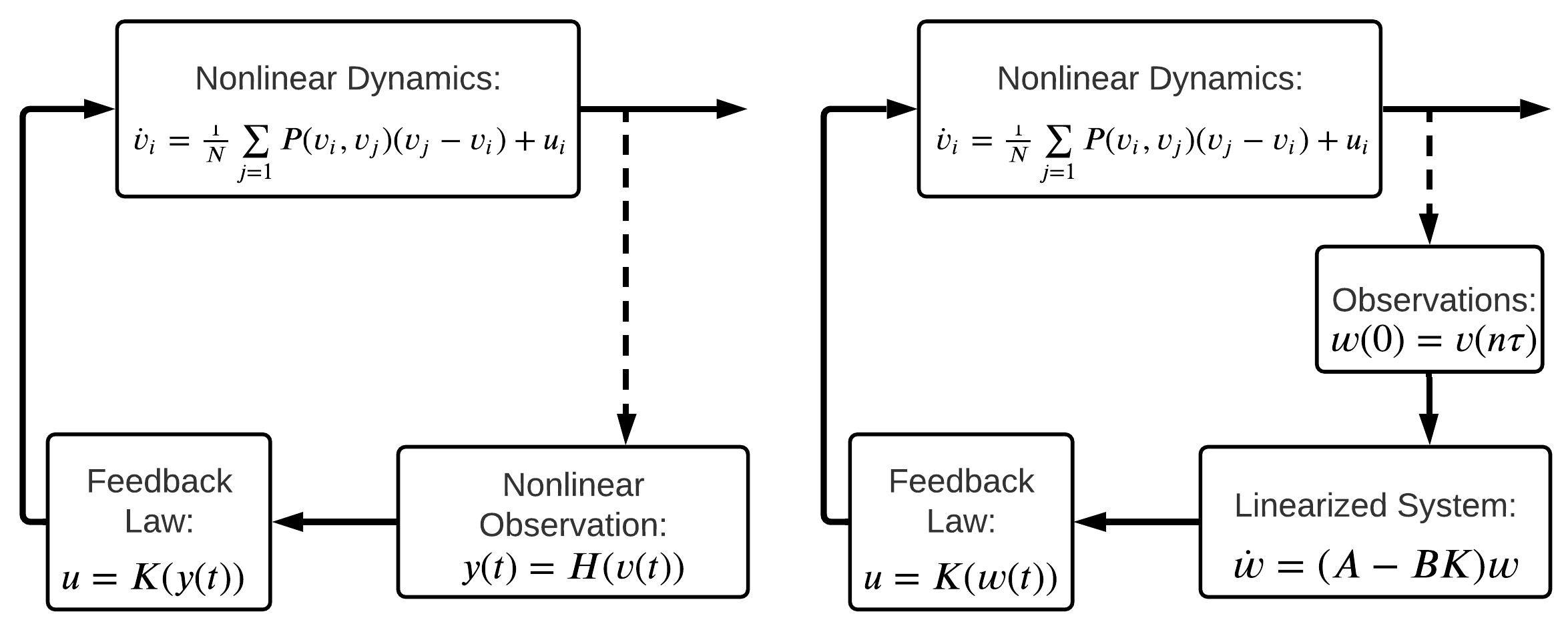
In order to circumvent these difficulties we propose an approach where we synthesize sub-optimal feedback-type controls through the linearization of the interaction kernel and by solving the resulting linear-quadratic optimal control problem through a Riccati equation – all based on the corresponding mean-field equations, similarly as in [51, 49]. This approach also avoids the limitations associated to the synthesis of optimal feedback laws for high-dimensional nonlinear dynamics via the Hamilton-Jacobi-Bellman PDE [33, 9]. The proposed methodology yields a control law for the linear model, which is later embedded into the non-linear dynamics (1.1). A sketch of this control concept is given in Figure 1.1 where we show the microscopic formulation of our approach. The main advantage of the proposed design is that unlike the classical control loop (1.1, left), we do not require a continuous measurement/estimation of the nonlinear state, nor the synthesis of a nonlinear optimal feedback law. Instead, we only require periodic measurements of the nonlinear state to update our linearized system.
Refer to caption
Figure 1.1: Left: the classical control loop for nonlinear dynamics. An often incomplete measurement of the state is recovered through a nonlinear observation. This observed state is inserted into a feedback law which requires the solution of a high-dimensional HJB PDE. This task is often unaffordable, and this block is replaced by a sub-optimal control law which is fed into the dynamics. Right: the Moment-driven predictive control methodology (MdPC) we propose simplifies the control loop on the left by requiring fewer measurements of the nonlinear state (every τ𝜏\tau seconds), feeding this information into a linearized system for which the optimal feedback law can be easily computed.

However, using the linear optimal control within the nonlinear model does not necessarily yield a stabilizing control law, since over time the nonlinear dynamics may be far from the linearization point. Because of the latter, we aim at quantifying the impact of this control and the number of linearization updates needed to stabilize the nonlinear system. Hence, we propose different controls, distinguishing between closed-loop and open-loop strategies: in the first case the control acts having access to the full information of the non-linear system at each time. In the second case, the control only requires information available at initial time. We quantify the performances of these control approaches by estimating the decay of macroscopic quantities associated to (1.1) such as the first and second moments of the particle ensemble.

In order to enhance open-loop strategies we introduce a novel Moment-driven Predictive Control (MdPC) framework. Based on dynamic estimates of the moments decay, we are able to perform a forward error analysis to estimate the next point in time where we need to update the linearization the dynamics and its feedback law. This strategy can be seen as model predictive control (MPC) technique [57, 20, 45, 10], where an open-loop control signal is applied only up to a subsequent point in time, after which the optimization is repeated. Moreover, the proposed control strategy is capable of treating efficiently high-dimensional control problems, and is robust in the case of limited access to the state and can be implemented with a small number of updates.

The rest of the paper is organized as follows. In Section 2 we derive different control systems based on the linearization of the dynamics and the solution of the Riccati equation associated to the linear-quadratic optimal control problem. Section 3 is devoted to the mean-field approximation of the microscopic dynamics and presents bounds for the moments decay. In Section 4 the Moment-driven Predictive Control framework is described and two different implementations are presented. Finally, in Section 5 we assess the proposed design via numerical experiments, showing different applications in the context of opinion formation and alignment dynamics.

2 Control of an interacting multi-agent system

In this section we present a linearization-based approach for the control of large-scale interacting particle systems. We are concerned with the evolution of N𝑁N interacting agents, whose states vi(t)dsubscript𝑣𝑖𝑡superscript𝑑v_{i}(t)\in\mathbb{R}^{d} evolve according to the following nonlinear model (1.1). Further assumptions regarding the interaction kernel P(u,v)𝑃𝑢𝑣P(u,v) governing these interactions will be discussed in the forthcoming sections. The term uidsubscript𝑢𝑖superscript𝑑u_{i}\in\mathbb{R}^{d} represents an external control variable acting over the ilimit-from𝑖i-th agent of the system. The complete set of control variables is denoted by u=(u1,,uN)N×d𝑢subscript𝑢1subscript𝑢𝑁superscript𝑁𝑑u=(u_{1},\ldots,u_{N})\in\mathbb{R}^{N\times d}. In order to synthesize this control variable, we assume that u𝑢u is the minimizer of a cost function J(u;v(0))𝐽𝑢𝑣0J(u;v(0)), that is

(2.1) u=argminuJ(u;v0):=0T(v(t),u(t))𝑑t,subject to (1.1).formulae-sequencesuperscript𝑢subscript𝑢𝐽𝑢superscript𝑣0assignsuperscriptsubscript0𝑇𝑣𝑡𝑢𝑡differential-d𝑡subject to (1.1)\displaystyle u^{*}=\arg\min_{u}J(u;v^{0}):=\int_{0}^{T}\ell(v(t),u(t))\,dt\,,\qquad\text{subject to \eqref{nonlin_dynamics}}\,.

The optimization horizon T𝑇T expresses the time scale along which we minimize the running cost (v,u)𝑣𝑢\ell(v,u), encodes our objective as a function of the state and control variables. In the context of this work, we are interested in consensus equilibrium, namely, reaching a consensus velocity v~d~𝑣superscript𝑑\tilde{v}\in\mathbb{R}^{d} such that v1==vN=v~subscript𝑣1subscript𝑣𝑁~𝑣v_{1}=\ldots=v_{N}=\tilde{v}. With a slight abuse of notation, we shall denote indistinctively by v~~𝑣\tilde{v} the consensus state and the swarm configuration v~N×d~𝑣superscript𝑁𝑑\tilde{v}\in\mathbb{R}^{N\times d} where all the agents share the same velocity. In order to promote consensus emergence, we solve the optimal control problem (2.1) to determine a control law u𝑢u driving the system towards v~~𝑣\tilde{v} using the running cost

(2.2) (v,u)=1Nj=1N(|vjv~|2+ν|uj|2)𝑣𝑢1𝑁superscriptsubscript𝑗1𝑁superscriptsubscript𝑣𝑗~𝑣2𝜈superscriptsubscript𝑢𝑗2\displaystyle\ell(v,u)=\frac{1}{N}\sum_{j=1}^{N}(|v_{j}-\tilde{v}|^{2}+\nu|u_{j}|^{2})

where ν>0𝜈0\nu>0 is a penalization parameter for the control energy, and v~~𝑣\tilde{v} is a prescribed consensus point. The norm |||\cdot| is the usual Euclidean norm in dsuperscript𝑑\mathbb{R}^{d}.

2.1 Linearization and the LQR approach for collective dynamics

We are interested in the synthesis of a feedback control law for the control of the non-linear dynamics (1.1). We begin by defining the vector-valued function F(v):N×dN×d:𝐹𝑣superscript𝑁𝑑superscript𝑁𝑑F(v):\mathbb{R}^{N\times d}\rightarrow\mathbb{R}^{N\times d} such that

(2.3) Fi(v)=1Nj=1NP(vi,vj)(vjvi),i=1,,N.formulae-sequencesubscript𝐹𝑖𝑣1𝑁superscriptsubscript𝑗1𝑁𝑃subscript𝑣𝑖subscript𝑣𝑗subscript𝑣𝑗subscript𝑣𝑖𝑖1𝑁F_{i}(v)=\frac{1}{N}\sum_{j=1}^{N}P(v_{i},v_{j})(v_{j}-v_{i}),\qquad i=1,\ldots,N.

We linearize the dynamics around vi=v¯subscript𝑣𝑖¯𝑣v_{i}=\bar{v} for every agent, which corresponds to an arbitrary equilibrium for the nonlinear dynamics (1.1), i.e. F(v¯)=0𝐹¯𝑣0F(\bar{v})=0, and which can be different from the consensus state v~~𝑣\tilde{v}. We further assume that the communication function P(vi,vj)𝑃subscript𝑣𝑖subscript𝑣𝑗P(v_{i},v_{j}) is such that P(v¯,v¯)p¯,𝑃¯𝑣¯𝑣¯𝑝P(\bar{v},\bar{v})\equiv\bar{p}\,, with p¯¯𝑝\bar{p} a bounded value. Computing the first order approximation of F(v)𝐹𝑣F(v) around v¯¯𝑣\bar{v}, we have vF(v¯)(vv¯)=A(vv¯),subscript𝑣𝐹¯𝑣𝑣¯𝑣𝐴𝑣¯𝑣\nabla_{v}F(\bar{v})(v-\bar{v})=A(v-\bar{v})\,, where AN×N𝐴superscript𝑁𝑁A\in\mathbb{R}^{N\times N} is the Laplacian matrix defined as follows

(2.4) (A)ij={ad=p¯(1N)N,i=j,ao=p¯N,ij.subscript𝐴𝑖𝑗casesotherwiseformulae-sequencesubscript𝑎𝑑¯𝑝1𝑁𝑁𝑖𝑗otherwiseformulae-sequencesubscript𝑎𝑜¯𝑝𝑁𝑖𝑗\displaystyle(A)_{ij}=\begin{cases}&a_{d}=\frac{\bar{p}(1-N)}{N},\qquad i=j,\\ &a_{o}=\frac{\bar{p}}{N},\qquad\qquad i\neq j.\\ \end{cases}

We observe that the structure of matrix A𝐴A is such that A(vv¯)=Av𝐴𝑣¯𝑣𝐴𝑣A(v-\bar{v})=Av since v¯¯𝑣\bar{v} is a consensus point. To write the linearized system associated to (1.1) we further consider the change of variables wi(t):=vi(t)v¯assignsubscript𝑤𝑖𝑡subscript𝑣𝑖𝑡¯𝑣w_{i}(t):=v_{i}(t)-\bar{v}, and we have

(2.5) w˙i=1Nj=1Np¯(wjwi)+ui,wi(0)=vi0v¯.formulae-sequencesubscript˙𝑤𝑖1𝑁superscriptsubscript𝑗1𝑁¯𝑝subscript𝑤𝑗subscript𝑤𝑖subscript𝑢𝑖subscript𝑤𝑖0superscriptsubscript𝑣𝑖0¯𝑣\dot{w}_{i}=\frac{1}{N}\sum_{j=1}^{N}\bar{p}(w_{j}-w_{i})+u_{i},\qquad\quad w_{i}(0)=v_{i}^{0}-\bar{v}.

For the linearized dynamics we cast as the Linear Quadratic Regulator (LQR) control problem, where the functional (2.1) reads as follows

(2.6) J(u,w(0))=0TwQw+νuRudt𝐽𝑢𝑤0superscriptsubscript0𝑇superscript𝑤top𝑄𝑤𝜈superscript𝑢top𝑅𝑢𝑑𝑡\displaystyle J(u,w(0))=\int_{0}^{T}w^{\top}Qw+\nu u^{\top}Ru\,dt

in the matrix-vector notation with w=(w1,,wN)𝑤subscript𝑤1subscript𝑤𝑁w=(w_{1},\ldots,w_{N}) and matrices QR=1NIdN×N𝑄𝑅1𝑁Idsuperscript𝑁𝑁Q\equiv R=\frac{1}{N}\textrm{Id}\in\mathbb{R}^{N\times N}. The linear dynamics (2.5) are equivalent to

(2.7) w˙=Aw+Bu,w(0)=v0v¯,formulae-sequence˙𝑤𝐴𝑤𝐵𝑢𝑤0superscript𝑣0¯𝑣\displaystyle\dot{w}=Aw+Bu,\qquad w(0)=v^{0}-\bar{v}\,,

where B=IdN×N𝐵Idsuperscript𝑁𝑁B=\textrm{Id}\in\mathbb{R}^{N\times N} is the identity matrix, impliying that the pair (A,B)𝐴𝐵(A,B) is controllable for any consensus state v¯¯𝑣\bar{v}. Thus, in a neighbourhood of any constant state v¯¯𝑣\bar{v} the non linear system (1.1) admits a continuous stabilizing feedback, see e.g. [17]. In order to synthesize a stabilizing control law we solve the optimal control problem (2.6)–(2.7), whose exact solution is given in feedback form by

(2.8) u(t)=NνK(t)w(t)𝑢𝑡𝑁𝜈𝐾𝑡𝑤𝑡\displaystyle u(t)=-\frac{N}{\nu}K(t)w(t)

with K(t)N×N𝐾𝑡superscript𝑁𝑁K(t)\in\mathbb{R}^{N\times N} fulfilling the Differential Riccati matrix-equation

(2.9) K˙=KA+AKNνKK+Q,K(T)=0N×N,formulae-sequence˙𝐾𝐾𝐴superscript𝐴top𝐾𝑁𝜈𝐾𝐾𝑄𝐾𝑇0superscript𝑁𝑁-\dot{K}=KA+A^{\top}K-\frac{N}{\nu}KK+Q,\quad K(T)=0\in\mathbb{R}^{N\times N},

coupled to the evolution of the controlled system (2.7). For a general linear system we need to solve the N×N𝑁𝑁N\times N differential system (2.9), which can be costly for large-scale agent-based dynamics. However, in this case we can exploit the symmetric structure of the Laplacian matrix A𝐴A to reduce the Riccati equation.

Proposition 2.1 (Properties of the Differential Riccati Equation).

For the linear dynamics (2.5), the solution of the Riccati equation (2.9) reduces to the solution of

(2.10a) kd˙˙subscript𝑘𝑑\displaystyle-\dot{k_{d}} =2kdad+2(N1)koaoNν(kd2+(N1)ko2)+1N,absent2subscript𝑘𝑑subscript𝑎𝑑2𝑁1subscript𝑘𝑜subscript𝑎𝑜𝑁𝜈superscriptsubscript𝑘𝑑2𝑁1superscriptsubscript𝑘𝑜21𝑁\displaystyle=2k_{d}a_{d}+2(N-1)k_{o}a_{o}-\frac{N}{\nu}\left(k_{d}^{2}+(N-1)k_{o}^{2}\right)+\frac{1}{N},
(2.10b) ko˙˙subscript𝑘𝑜\displaystyle-\dot{k_{o}} =2(N2)koao+2koad+2kdaoNν(2kdko+(N2)ko2),absent2𝑁2subscript𝑘𝑜subscript𝑎𝑜2subscript𝑘𝑜subscript𝑎𝑑2subscript𝑘𝑑subscript𝑎𝑜𝑁𝜈2subscript𝑘𝑑subscript𝑘𝑜𝑁2superscriptsubscript𝑘𝑜2\displaystyle=2(N-2)k_{o}a_{o}+2k_{o}a_{d}+2k_{d}a_{o}-\frac{N}{\nu}\left(2k_{d}k_{o}+(N-2)k_{o}^{2}\right),

with terminal conditions kd(T)=ko(T)=0subscript𝑘𝑑𝑇subscript𝑘𝑜𝑇0k_{d}(T)=k_{o}(T)=0. The solution K𝐾K of the differential Riccati equation (2.9) corresponds to (K)ij=δijkd+(1δij)kosubscript𝐾𝑖𝑗subscript𝛿𝑖𝑗subscript𝑘𝑑1subscript𝛿𝑖𝑗subscript𝑘𝑜(K)_{ij}=\delta_{ij}k_{d}+(1-\delta_{ij})k_{o}.

Proof.

Given the structure of the matrices K𝐾K, A𝐴A and Q𝑄Q, solving the Riccati equation (2.9) componentwise leads to the following identities:

Diagonal entries kii::Diagonal entries kiiabsent\displaystyle\text{Diagonal entries $k_{ii}$}:\qquad Nν(K2)ii=Nν(kd2+(N1)ko2).𝑁𝜈subscriptsuperscript𝐾2𝑖𝑖𝑁𝜈superscriptsubscript𝑘𝑑2𝑁1superscriptsubscript𝑘𝑜2\displaystyle\frac{N}{\nu}(K^{2})_{ii}=\frac{N}{\nu}\left(k_{d}^{2}+(N-1)k_{o}^{2}\right).
Off-diagonal entries kijsubscript𝑘𝑖𝑗k_{ij}: Nν(K2)ij=Nν(2kdko+(N2)ko2).𝑁𝜈subscriptsuperscript𝐾2𝑖𝑗𝑁𝜈2subscript𝑘𝑑subscript𝑘𝑜𝑁2superscriptsubscript𝑘𝑜2\displaystyle\frac{N}{\nu}(K^{2})_{ij}=\frac{N}{\nu}\left(2k_{d}k_{o}+(N-2)k_{o}^{2}\right).

We can further simplify the Riccati-matrix system (2.10) using the dependency of coefficients ad,aosubscript𝑎𝑑subscript𝑎𝑜a_{d},a_{o} (2.4) and the parameter p¯¯𝑝\bar{p}. This leads to

(2.11) k˙dsubscript˙𝑘𝑑\displaystyle-\dot{{k}}_{d} =2p¯(N1)N(kdko)Nν(kd2+(N1)ko2)+1N,kd(T)=0,formulae-sequenceabsent2¯𝑝𝑁1𝑁subscript𝑘𝑑subscript𝑘𝑜𝑁𝜈superscriptsubscript𝑘𝑑2𝑁1superscriptsubscript𝑘𝑜21𝑁subscript𝑘𝑑𝑇0\displaystyle=-\frac{2\bar{p}(N-1)}{N}({k}_{d}-k_{o})-\frac{N}{\nu}\left({k}_{d}^{2}+(N-1){k}_{o}^{2}\right)+\frac{1}{N},\qquad k_{d}(T)=0\,,
(2.12) k˙osubscript˙𝑘𝑜\displaystyle-\dot{{k}}_{o} =2p¯N(kdko)Nν(2kdko+(N2)ko2),ko(T)=0.formulae-sequenceabsent2¯𝑝𝑁subscript𝑘𝑑subscript𝑘𝑜𝑁𝜈2subscript𝑘𝑑subscript𝑘𝑜𝑁2superscriptsubscript𝑘𝑜2subscript𝑘𝑜𝑇0\displaystyle=\frac{2\bar{p}}{N}(k_{d}-k_{o})-\frac{N}{\nu}\left(2{k}_{d}{k}_{o}+(N-2){k}_{o}^{2}\right),\qquad k_{o}(T)=0.

Since we are interested in the dynamics for large number of agents, we introduce the following scalings

(2.13) kdNkd,koN2ko,α(N)=N1N.formulae-sequencesubscript𝑘𝑑𝑁subscript𝑘𝑑formulae-sequencesubscript𝑘𝑜superscript𝑁2subscript𝑘𝑜𝛼𝑁𝑁1𝑁{k}_{d}\leftarrow Nk_{d},\quad{k}_{o}\leftarrow N^{2}k_{o},\quad\alpha(N)=\frac{N-1}{N}.

For the sake of simplicity, we keep the same notation also for the scaled variables kd,kosubscript𝑘𝑑subscript𝑘𝑜k_{d},k_{o}. Under this scaling the system (2.11)–(2.12) reads

(2.14) k˙dsubscript˙𝑘𝑑\displaystyle-\dot{k}_{d} =2p¯α(N)(kdkoN)1ν(kd2+α(N)Nko2)+1,kd(T)=0,formulae-sequenceabsent2¯𝑝𝛼𝑁subscript𝑘𝑑subscript𝑘𝑜𝑁1𝜈superscriptsubscript𝑘𝑑2𝛼𝑁𝑁superscriptsubscript𝑘𝑜21subscript𝑘𝑑𝑇0\displaystyle=-2\bar{p}\alpha(N)\left(k_{d}-\frac{k_{o}}{N}\right)-\frac{1}{\nu}\left(k_{d}^{2}+\frac{\alpha(N)}{N}k_{o}^{2}\right)+1,\qquad k_{d}(T)=0,
(2.15) k˙osubscript˙𝑘𝑜\displaystyle-\dot{k}_{o} =2p¯(kdkoN)1ν(2kdko+α(N)ko21Nko2),ko(T)=0,formulae-sequenceabsent2¯𝑝subscript𝑘𝑑subscript𝑘𝑜𝑁1𝜈2subscript𝑘𝑑subscript𝑘𝑜𝛼𝑁superscriptsubscript𝑘𝑜21𝑁superscriptsubscript𝑘𝑜2subscript𝑘𝑜𝑇0\displaystyle=2\bar{p}\left(k_{d}-\frac{k_{o}}{N}\right)-\frac{1}{\nu}\left(2k_{d}k_{o}+\alpha(N)k_{o}^{2}-\frac{1}{N}k_{o}^{2}\right),\qquad k_{o}(T)=0\,,

and the Riccati feedback law (2.8) is given by

(2.16) uisubscript𝑢𝑖\displaystyle u_{i} =1ν((kdkoN)wi(t)+koNj=1Nwj(t)).absent1𝜈subscript𝑘𝑑subscript𝑘𝑜𝑁subscript𝑤𝑖𝑡subscript𝑘𝑜𝑁superscriptsubscript𝑗1𝑁subscript𝑤𝑗𝑡\displaystyle=-\frac{1}{\nu}\left(\left(k_{d}-\frac{k_{o}}{N}\right)w_{i}(t)+\frac{k_{o}}{N}\sum_{j=1}^{N}w_{j}(t)\right)\,.

Plugging the control into the linear dynamics (2.5) and rearranging the terms we have

(2.17) w˙isubscript˙𝑤𝑖\displaystyle\dot{w}_{i} =(p¯koν)1Nj=1Nwj(p¯+kdνkoνN)wi,wi(0)=vi0v¯.formulae-sequenceabsent¯𝑝subscript𝑘𝑜𝜈1𝑁superscriptsubscript𝑗1𝑁subscript𝑤𝑗¯𝑝subscript𝑘𝑑𝜈subscript𝑘𝑜𝜈𝑁subscript𝑤𝑖subscript𝑤𝑖0superscriptsubscript𝑣𝑖0¯𝑣\displaystyle=\left(\bar{p}-\frac{k_{o}}{\nu}\right)\frac{1}{N}\sum_{j=1}^{N}w_{j}-\left(\bar{p}+\frac{k_{d}}{\nu}-\frac{k_{o}}{\nu N}\right)w_{i},\qquad w_{i}(0)=v_{i}^{0}-\bar{v}.

The controlled dynamics (2.17) are non-autonomous as the coefficients kd(t),ko(t)subscript𝑘𝑑𝑡subscript𝑘𝑜𝑡k_{d}(t),k_{o}(t), have to be determined offline by solving (2.14)–(2.15) backwards in time.

In order to analyse the large-scale behaviour of the system we introduce the average of the agent states, and a weighted combination of the Riccati coefficients, respectively

mwN(t):=1Nj=1Nwj(t),s(t):=kd(t)+α(N)ko(t).formulae-sequenceassignsuperscriptsubscript𝑚𝑤𝑁𝑡1𝑁superscriptsubscript𝑗1𝑁subscript𝑤𝑗𝑡assign𝑠𝑡subscript𝑘𝑑𝑡𝛼𝑁subscript𝑘𝑜𝑡\displaystyle m_{w}^{N}(t):=\frac{1}{N}\sum_{j=1}^{N}w_{j}(t),\quad s(t):=k_{d}(t)+\alpha(N)k_{o}(t).

From (2.17), (2.14) and (2.15), these quantities are governed by

(2.18a) m˙wN(t)superscriptsubscript˙𝑚𝑤𝑁𝑡\displaystyle\dot{m}_{w}^{N}(t) =1νs(t)mwN(t),mwN(0)=mvN(0)v¯,formulae-sequenceabsent1𝜈𝑠𝑡superscriptsubscript𝑚𝑤𝑁𝑡subscriptsuperscript𝑚𝑁𝑤0subscriptsuperscript𝑚𝑁𝑣0¯𝑣\displaystyle=-\frac{1}{\nu}s(t)m_{w}^{N}(t),\qquad m^{N}_{w}(0)=m^{N}_{v}(0)-\bar{v},
(2.18b) s˙(t)˙𝑠𝑡\displaystyle-\dot{s}(t) =11νs(t)2,s(T)=0.formulae-sequenceabsent11𝜈𝑠superscript𝑡2𝑠𝑇0\displaystyle=1-\frac{1}{\nu}s(t)^{2},\qquad\quad s(T)=0.

The second equation has an explicit solution s(t)=νtanh((Tt)/ν)𝑠𝑡𝜈𝑇𝑡𝜈s(t)=\sqrt{\nu}\tanh((T-t)/\sqrt{\nu}), always non-negative for t[0,T]𝑡0𝑇t\in[0,T] [51]. The average mvN(t)subscriptsuperscript𝑚𝑁𝑣𝑡m^{N}_{v}(t) follows a relaxation towards v¯¯𝑣\bar{v}

(2.19) m˙vN(t)=1νtanh(Ttν)(mvN(t)v¯).superscriptsubscript˙𝑚𝑣𝑁𝑡1𝜈𝑇𝑡𝜈superscriptsubscript𝑚𝑣𝑁𝑡¯𝑣\displaystyle\dot{m}_{v}^{N}(t)=-\frac{1}{\sqrt{\nu}}\tanh\left(\frac{T-t}{\sqrt{\nu}}\right)(m_{v}^{N}(t)-\bar{v}).
Remark 2.1 (Second order dynamics).

This approach can be extended to second order models [27, 35, 58]. Here, the state space of a swarm of N𝑁N agents is characterized by position and velocities (xi(t),vi(t))i2×dsubscriptsubscript𝑥𝑖𝑡subscript𝑣𝑖𝑡𝑖superscript2𝑑(x_{i}(t),v_{i}(t))_{i}\in\mathbb{R}^{2\times d}, evolving according to

(2.20) x˙i=vi,v˙i=1Nj=1NP(xi,xj)(vjvi)+ui,i=1,,N.formulae-sequencesubscript˙𝑥𝑖subscript𝑣𝑖formulae-sequencesubscript˙𝑣𝑖1𝑁superscriptsubscript𝑗1𝑁𝑃subscript𝑥𝑖subscript𝑥𝑗subscript𝑣𝑗subscript𝑣𝑖subscript𝑢𝑖𝑖1𝑁\dot{x}_{i}=v_{i},\qquad\dot{v}_{i}=\frac{1}{N}\sum_{j=1}^{N}P(x_{i},x_{j})(v_{j}-v_{i})+u_{i},\qquad i=1,\ldots,N\,.

where uN×d𝑢superscript𝑁𝑑u\in\mathbb{R}^{N\times d}. We consider again a functional of type (2.2), where we enforce a consensus point vi=vj=v~subscript𝑣𝑖subscript𝑣𝑗~𝑣v_{i}=v_{j}=\tilde{v} for every i,j𝑖𝑗i,j. Linearizing around this point and introducing the shift yi=xiv¯t,wi=viv¯formulae-sequencesubscript𝑦𝑖subscript𝑥𝑖¯𝑣𝑡subscript𝑤𝑖subscript𝑣𝑖¯𝑣y_{i}=x_{i}-\bar{v}t,\quad w_{i}=v_{i}-\bar{v}, the system is transformed into

(2.21) [y˙w˙]=[0Id0A][yw]+[0Id]u.matrix˙𝑦˙𝑤matrix0Id0𝐴matrix𝑦𝑤matrix0Id𝑢\begin{bmatrix}\dot{y}\\ \dot{w}\end{bmatrix}=\begin{bmatrix}0&\textrm{Id}\\ 0&A\end{bmatrix}\begin{bmatrix}y\\ w\end{bmatrix}+\begin{bmatrix}0\\ \textrm{Id}\end{bmatrix}u\,.

This second-order system system is controllable [49], and the associated Differential Riccati Equation reads

(2.22) [K˙11K˙12K˙21K˙22]=matrixsubscript˙𝐾11subscript˙𝐾12subscript˙𝐾21subscript˙𝐾22absent\displaystyle\begin{bmatrix}\dot{K}_{11}&\dot{K}_{12}\\ \dot{K}_{21}&\dot{K}_{22}\end{bmatrix}= [000K21+K22A]+[00K11+AK21K12+AK22]matrix000subscript𝐾21subscript𝐾22𝐴matrix00subscript𝐾11𝐴subscript𝐾21subscript𝐾12𝐴subscript𝐾22\displaystyle\begin{bmatrix}0&0\\ 0&K_{21}+K_{22}A\end{bmatrix}+\begin{bmatrix}0&0\\ K_{11}+AK_{21}&K_{12}+AK_{22}\end{bmatrix}
Nν[K12K21K12K22K22K21(K22)2]+[000Id],𝑁𝜈matrixsubscript𝐾12subscript𝐾21subscript𝐾12subscript𝐾22subscript𝐾22subscript𝐾21superscriptsubscript𝐾222matrix000Id\displaystyle-\frac{N}{\nu}\begin{bmatrix}K_{12}K_{21}&K_{12}K_{22}\\ K_{22}K_{21}&(K_{22})^{2}\end{bmatrix}+\begin{bmatrix}0&0\\ 0&\textrm{Id}\end{bmatrix},

with terminal conditions Kij(T)=0subscript𝐾𝑖𝑗𝑇0K_{ij}(T)=0, for i,j=1,2formulae-sequence𝑖𝑗12\ i,j=1,2. This system is easily solved with K11=K12=K21=0subscript𝐾11subscript𝐾12subscript𝐾210K_{11}=K_{12}=K_{21}=0 and K22subscript𝐾22K_{22} satisfying a Riccati equation equivalent to (2.9). Hence, the results we obtain for the first order system can be extended to second order systems. We will further discuss this extension in the numerical section.

2.2 Riccati-based control laws for the non-linear system

In order to approximate the synthesis of feedback laws for the original nonlinear optimal control problem (2.1), we study sub-optimal stabilizing strategies induced by the Riccati control (2.8). Without loss of generality, we will consider the stabilization problem towards v~=0~𝑣0\tilde{v}=0. We will focus on different ways to synthesize a control law based on the information retrieved in the linearized case: a closed-loop control, an open-loop strategy, and a simplified inexact open-loop control.

Closed-loop control

A well-known local strategy for the control of nonlinear dynamics is to use the optimal feedback control obtained from the linearized dynamics. In this case, the controlled system reads

(2.23) v˙i=1Nj=1NP(vi,vj)(vjvi)+Ri[v](t),vi(0)=vi0,formulae-sequencesubscript˙𝑣𝑖1𝑁superscriptsubscript𝑗1𝑁𝑃subscript𝑣𝑖subscript𝑣𝑗subscript𝑣𝑗subscript𝑣𝑖subscript𝑅𝑖delimited-[]𝑣𝑡subscript𝑣𝑖0subscriptsuperscript𝑣0𝑖\dot{v}_{i}=\frac{1}{N}\sum_{j=1}^{N}P(v_{i},v_{j})(v_{j}-v_{i})+R_{i}[v](t),\qquad v_{i}(0)=v^{0}_{i},

where the operator Ri[]subscript𝑅𝑖delimited-[]R_{i}[\cdot] is the feedback (2.8) applied directly to the state of the non-linear system v(t)=(vi(t))i=1N𝑣𝑡superscriptsubscriptsubscript𝑣𝑖𝑡𝑖1𝑁v(t)=(v_{i}(t))_{i=1}^{N}, namely

(2.24) Ri[v](t)subscript𝑅𝑖delimited-[]𝑣𝑡\displaystyle R_{i}[v](t) =1ν((kd(t)ko(t)N)vi(t)+ko(t)Nj=1Nvj(t)),absent1𝜈subscript𝑘𝑑𝑡subscript𝑘𝑜𝑡𝑁subscript𝑣𝑖𝑡subscript𝑘𝑜𝑡𝑁superscriptsubscript𝑗1𝑁subscript𝑣𝑗𝑡\displaystyle=-\frac{1}{\nu}\left(\left(k_{d}(t)-\frac{k_{o}(t)}{N}\right)v_{i}(t)+\frac{k_{o}(t)}{N}\sum_{j=1}^{N}v_{j}(t)\right),

where kd(t),ko(t)subscript𝑘𝑑𝑡subscript𝑘𝑜𝑡k_{d}(t),k_{o}(t) are still obtained by solving the system (2.14)–(2.15). In general, such a control law is expected to work only for initial states sufficiently close to the state around which the dynamics have been linearised. We shall investigate in detail the properties of the closed-loop in the following section.

Open-loop control

The open-loop strategy we propose applies the control signal obtained from the linear synthesis ui(t;v0)subscript𝑢𝑖𝑡superscript𝑣0u_{i}(t;v^{0}) directly into the the non-linear dynamics as follows

(2.25a) v˙isubscript˙𝑣𝑖\displaystyle\dot{v}_{i} =1Nj=1NP(vi,vj)(vjvi)+Ri[w](t),vi(0)=vi0,formulae-sequenceabsent1𝑁superscriptsubscript𝑗1𝑁𝑃subscript𝑣𝑖subscript𝑣𝑗subscript𝑣𝑗subscript𝑣𝑖subscript𝑅𝑖delimited-[]𝑤𝑡subscript𝑣𝑖0subscriptsuperscript𝑣0𝑖\displaystyle=\frac{1}{N}\sum\limits_{j=1}^{N}P(v_{i},v_{j})(v_{j}-v_{i})+R_{i}[w](t),\qquad v_{i}(0)=v^{0}_{i},
(2.25b) w˙isubscript˙𝑤𝑖\displaystyle\dot{w}_{i} =1Nj=1Np¯(wjwi)+Ri[w](t),wi(0)=vi0,formulae-sequenceabsent1𝑁superscriptsubscript𝑗1𝑁¯𝑝subscript𝑤𝑗subscript𝑤𝑖subscript𝑅𝑖delimited-[]𝑤𝑡subscript𝑤𝑖0subscriptsuperscript𝑣0𝑖\displaystyle=\frac{1}{N}\sum\limits_{j=1}^{N}\bar{p}(w_{j}-w_{i})+R_{i}[w](t),\qquad\quad\qquad w_{i}(0)=v^{0}_{i},

where the control Ri[w](t)subscript𝑅𝑖delimited-[]𝑤𝑡R_{i}[w](t) is computed according to (2.8). This approach is open-loop, since all the information on the state of the non-linear system reduces to the initial state of linearized system, assuming wi0=vi0subscriptsuperscript𝑤0𝑖subscriptsuperscript𝑣0𝑖w^{0}_{i}=v^{0}_{i}. While this approach is clearly outperformed by the closed-loop feedback law in terms of robustness, it has the advantage that it can be implemented without requiring a continuous measurement of the full nonlinear state v(t)𝑣𝑡v(t), making it appealing for systems where recovering the true state of the dynamics can be expensive or time-consuming.

Inexact open-loop control

An inexact, but simpler, implementation of the open-loop approach (2.25) obtained when the control Ri[]subscript𝑅𝑖delimited-[]R_{i}[\cdot] is evaluated only with respect to the initial data vi0subscriptsuperscript𝑣0𝑖v^{0}_{i}, that is Ri[v0](t)subscript𝑅𝑖delimited-[]superscript𝑣0𝑡R_{i}[v^{0}](t), where the dependence on t𝑡t is limited to ko(t)subscript𝑘𝑜𝑡k_{o}(t) and kd(t)subscript𝑘𝑑𝑡k_{d}(t). This setting avoids the evaluation of system in (2.25), and only requires the computation of

(2.26) v˙i=1Nj=1NP(vi,vj)(vjvi)+Ri[v0](t),vi(0)=vi0.formulae-sequencesubscript˙𝑣𝑖1𝑁superscriptsubscript𝑗1𝑁𝑃subscript𝑣𝑖subscript𝑣𝑗subscript𝑣𝑗subscript𝑣𝑖subscript𝑅𝑖delimited-[]superscript𝑣0𝑡subscript𝑣𝑖0subscriptsuperscript𝑣0𝑖\dot{v}_{i}=\frac{1}{N}\sum_{j=1}^{N}P(v_{i},v_{j})(v_{j}-v_{i})+R_{i}[v^{0}](t),\qquad v_{i}(0)=v^{0}_{i}.

The open-loop control laws are meant to be embedded in a Model Predictive Control framework, ensuring a sufficiently frequent update of the state of the nonlinear system ensuring stability of the resulting control system. This shall be further analysed in Section 4. In the following section we will study the performance of these control strategies when stabilizing the non-linear dynamics in the case N1much-greater-than𝑁1N\gg 1.

3 Mean-field limits and moments estimates

The stabilization strategies (2.23) and (2.25) are clearly suboptimal with respect to the original optimal control problem, and in general will not guarantee the stabilization of the non-linear dynamics (1.1). In this section we quantify the discrepancy between the desired target state and the final state obtained by the stabilization strategies (2.23) and (2.25). In order to estimate these performances in the case where a large number of agents is present, i.e. N1much-greater-than𝑁1N\gg 1, we discuss our approaches in the mean-field limit. Here, we consider the density distribution of agents in order to describe the collective behavior of the ensemble of particles, and we retrieve upper and lower bounds for the decay of the mean-field density towards the desired configuration.

3.1 Open-loop Riccati control

We introduce the empirical joint probability distribution of particles for the system (1.1) and (2.5) is given by

(3.1) λN(t,v,w)=1Ni=1Nδ(vvi(t))δ(wwi(t)),superscript𝜆𝑁𝑡𝑣𝑤1𝑁superscriptsubscript𝑖1𝑁𝛿𝑣subscript𝑣𝑖𝑡𝛿𝑤subscript𝑤𝑖𝑡\lambda^{N}(t,v,w)=\frac{1}{N}\sum_{i=1}^{N}\delta(v-v_{i}(t))\delta(w-w_{i}(t)),

where δ()𝛿\delta(\cdot) is a Dirac measure. We assume enough regularity on the interaction kernel, assuming that particles remain in a fixed compact domain for all N𝑁N and in the whole time interval [0,T]0𝑇[0,T]. We refer to [21, 23] for a rigorous treatment of the mean-field limit of interacting particle systems. Hence, we introduce the test function ϕ(v,w)C01(2d)italic-ϕ𝑣𝑤subscriptsuperscript𝐶10superscript2𝑑\phi(v,w)\in C^{1}_{0}(\mathbb{R}^{2d}) and by Liouville’s theorem we compute the time variation of the inner-product λN(t),ϕsuperscript𝜆𝑁𝑡italic-ϕ\langle\lambda^{N}(t),\phi\rangle, given by

(3.2) ddtλN(t),ϕ=1Ni=1N(vϕ(vi,wi)v˙i(t)+wϕ(vi,wi)w˙i(t)).𝑑𝑑𝑡superscript𝜆𝑁𝑡italic-ϕ1𝑁superscriptsubscript𝑖1𝑁subscript𝑣italic-ϕsubscript𝑣𝑖subscript𝑤𝑖subscript˙𝑣𝑖𝑡subscript𝑤italic-ϕsubscript𝑣𝑖subscript𝑤𝑖subscript˙𝑤𝑖𝑡\frac{d}{dt}\langle\lambda^{N}(t),\phi\rangle=\frac{1}{N}\sum_{i=1}^{N}(\nabla_{v}\phi(v_{i},w_{i})\cdot\dot{v}_{i}(t)+\nabla_{w}\phi(v_{i},w_{i})\cdot\dot{w}_{i}(t)).

Denoting by λN(t):=λN(t,v,w)assignsuperscript𝜆𝑁𝑡superscript𝜆𝑁𝑡𝑣𝑤\lambda^{N}(t):=\lambda^{N}(t,v,w), we define the marginal densities fNsuperscript𝑓𝑁f^{N}, gNsuperscript𝑔𝑁g^{N}, the average m1[fN]subscript𝑚1delimited-[]superscript𝑓𝑁m_{1}[f^{N}] and the second moment m2[fN]subscript𝑚2delimited-[]superscript𝑓𝑁m_{2}[f^{N}] as follows

(3.3) fN(t,w)superscript𝑓𝑁𝑡𝑤\displaystyle f^{N}(t,w) :=dλN(t,v,w)𝑑v,gN(t,v):=dλN(t,v,w)𝑑w;formulae-sequenceassignabsentsubscriptsuperscript𝑑superscript𝜆𝑁𝑡𝑣𝑤differential-d𝑣assignsuperscript𝑔𝑁𝑡𝑣subscriptsuperscript𝑑superscript𝜆𝑁𝑡𝑣𝑤differential-d𝑤\displaystyle:=\int_{\mathbb{R}^{d}}\lambda^{N}(t,v,w)dv,\qquad g^{N}(t,v):=\int_{\mathbb{R}^{d}}\lambda^{N}(t,v,w)dw;
m1[fN](t)subscript𝑚1delimited-[]superscript𝑓𝑁𝑡\displaystyle m_{1}[f^{N}](t) :=dwfN(t,w)𝑑w,m2[fN](t):=d|w|2fN(t,w)𝑑w.formulae-sequenceassignabsentsubscriptsuperscript𝑑𝑤superscript𝑓𝑁𝑡𝑤differential-d𝑤assignsubscript𝑚2delimited-[]superscript𝑓𝑁𝑡subscriptsuperscript𝑑superscript𝑤2superscript𝑓𝑁𝑡𝑤differential-d𝑤\displaystyle:=\int_{\mathbb{R}^{d}}wf^{N}(t,w)dw\,,\quad m_{2}[f^{N}](t):=\int_{\mathbb{R}^{d}}|w|^{2}f^{N}(t,w)dw\,.

With the standard derivation of the mean-field limit, we obtain in the strong form the evolution equation for λN(t,v,w)superscript𝜆𝑁𝑡𝑣𝑤\lambda^{N}(t,v,w) as follows

tλNsubscript𝑡superscript𝜆𝑁\displaystyle\partial_{t}\lambda^{N} =v[λN(𝒫[gN]aN(t)wbN(t)m1[fN])]absentsubscript𝑣delimited-[]superscript𝜆𝑁𝒫delimited-[]superscript𝑔𝑁superscript𝑎𝑁𝑡𝑤superscript𝑏𝑁𝑡subscript𝑚1delimited-[]superscript𝑓𝑁\displaystyle=-\nabla_{v}\cdot\left[\lambda^{N}\left(\mathcal{P}[g^{N}]-a^{N}(t)w-b^{N}(t)m_{1}[f^{N}]\right)\right]
w[λN(p¯(m1[f]w)aN(t)wbN(t)m1[fN])],subscript𝑤delimited-[]superscript𝜆𝑁¯𝑝subscript𝑚1delimited-[]𝑓𝑤superscript𝑎𝑁𝑡𝑤superscript𝑏𝑁𝑡subscript𝑚1delimited-[]superscript𝑓𝑁\displaystyle\qquad-\nabla_{w}\cdot\left[\lambda^{N}\left(\bar{p}(m_{1}[f]-w)-a^{N}(t)w-b^{N}(t)m_{1}[f^{N}]\right)\right],

where 𝒫[g]𝒫delimited-[]𝑔\mathcal{P}[g] denotes the nonlocal integral operator

𝒫[g](v,t)=dP(v,v)(vv)g(v,t)𝑑v,𝒫delimited-[]𝑔𝑣𝑡subscriptsuperscript𝑑𝑃𝑣subscript𝑣subscript𝑣𝑣𝑔subscript𝑣𝑡differential-dsubscript𝑣\mathcal{P}[g](v,t)=\int_{\mathbb{R}^{d}}P(v,v_{*})(v_{*}-v)g(v_{*},t)dv_{*},

and aN(t)superscript𝑎𝑁𝑡a^{N}(t) and bN(t)superscript𝑏𝑁𝑡b^{N}(t) are obtained from the scaled Riccati system (2.14)-(2.15). Since we are interested in the limit of a large number of agents, for N𝑁N\to\infty we have

limNaN(t)=kd(t)ν,limNbN(t)=ko(t)ν,formulae-sequencesubscript𝑁superscript𝑎𝑁𝑡subscript𝑘𝑑𝑡𝜈subscript𝑁superscript𝑏𝑁𝑡subscript𝑘𝑜𝑡𝜈\lim_{N\rightarrow\infty}a^{N}(t)=\frac{k_{d}(t)}{\nu},\qquad\lim_{N\rightarrow\infty}b^{N}(t)=\frac{k_{o}(t)}{\nu},

where kdsubscript𝑘𝑑k_{d} and kosubscript𝑘𝑜k_{o} fulfill

(3.4) k˙d=2p¯kdkd2ν+1,k˙o=2p¯kdkoν(2kd+ko).formulae-sequencesubscript˙𝑘𝑑2¯𝑝subscript𝑘𝑑superscriptsubscript𝑘𝑑2𝜈1subscript˙𝑘𝑜2¯𝑝subscript𝑘𝑑subscript𝑘𝑜𝜈2subscript𝑘𝑑subscript𝑘𝑜\displaystyle-\dot{k}_{d}=-2\bar{p}k_{d}-\frac{k_{d}^{2}}{\nu}+1,\qquad-\dot{k}_{o}=2\bar{p}k_{d}-\frac{k_{o}}{\nu}\left(2k_{d}+k_{o}\right)\,.

Then, the joint mean-field model can be conveniently written as

(3.5) tλsubscript𝑡𝜆\displaystyle\partial_{t}\lambda =v[λ(𝒫[g]kdνwkoνm1[f])]absentsubscript𝑣delimited-[]𝜆𝒫delimited-[]𝑔subscript𝑘𝑑𝜈𝑤subscript𝑘𝑜𝜈subscript𝑚1delimited-[]𝑓\displaystyle=-\nabla_{v}\cdot\left[\lambda\left(\mathcal{P}[g]-\frac{k_{d}}{\nu}w-\frac{k_{o}}{\nu}m_{1}[f]\right)\right]
w[λ(p¯(m1[f]w)kdνwkoνm1[f]))],\displaystyle\qquad\qquad-\nabla_{w}\cdot\left[\lambda\left(\bar{p}\left(m_{1}[f]-w\right)-\frac{k_{d}}{\nu}w-\frac{k_{o}}{\nu}m_{1}[f])\right)\right],

with intial data λ(v,w,0)=λ0(v,w)𝜆𝑣𝑤0superscript𝜆0𝑣𝑤\lambda(v,w,0)=\lambda^{0}(v,w). Integrating the mean-field equation (3.5) with respect to v𝑣v and w𝑤w, the evolution of the marginals f(w,t)𝑓𝑤𝑡f(w,t) and g(v,t)𝑔𝑣𝑡g(v,t) is given by

(3.6a) tg=v[g(𝒫[g]kdνm1[h]koνm1[f])],g(v,0)=g0(v)formulae-sequencesubscript𝑡𝑔subscript𝑣delimited-[]𝑔𝒫delimited-[]𝑔subscript𝑘𝑑𝜈subscript𝑚1delimited-[]subscript𝑘𝑜𝜈subscript𝑚1delimited-[]𝑓𝑔𝑣0superscript𝑔0𝑣\displaystyle\partial_{t}g=-\nabla_{v}\cdot\left[g\left(\mathcal{P}[g]-\frac{k_{d}}{\nu}m_{1}[h]-\frac{k_{o}}{\nu}m_{1}[f]\right)\right],\qquad\qquad\,\,g(v,0)=g^{0}(v)
(3.6b) tf=w[f((p¯koν)m1[f](p¯+kdν)w)],f(w,0)=g0(w)formulae-sequencesubscript𝑡𝑓subscript𝑤delimited-[]𝑓¯𝑝subscript𝑘𝑜𝜈subscript𝑚1delimited-[]𝑓¯𝑝subscript𝑘𝑑𝜈𝑤𝑓𝑤0superscript𝑔0𝑤\displaystyle\partial_{t}f=-\nabla_{w}\cdot\left[f\left(\left(\bar{p}-\frac{k_{o}}{\nu}\right)m_{1}[f]-\left(\bar{p}+\frac{k_{d}}{\nu}\right)w\right)\right],\qquad f(w,0)=g^{0}(w)

with m1[h](v,t)subscript𝑚1delimited-[]𝑣𝑡m_{1}[h](v,t) being the average of the conditional probabilty h(w|v,t)conditional𝑤𝑣𝑡h(w|v,t) defined as

(3.7) λ(t,v,w)=h(t,w|v)g(t,v),m1[h](t,v)=dwh(t,w|v)𝑑w.formulae-sequence𝜆𝑡𝑣𝑤𝑡conditional𝑤𝑣𝑔𝑡𝑣subscript𝑚1delimited-[]𝑡𝑣subscriptsuperscript𝑑𝑤𝑡conditional𝑤𝑣differential-d𝑤\displaystyle\lambda(t,v,w)=h(t,w|v)g(t,v),\qquad m_{1}[h](t,v)=\int_{\mathbb{R}^{d}}wh(t,w|v)dw.

We observe that equation (3.6b) is the mean-field equation associated to the linear controlled model (2.17) [51]. On the other hand, the equation for the non-linear model (3.6a) is coupled to the solution of the linear model through the control.

Remark 3.1 (Inexact mean-field open-loop control).

If we consider the inexact open-loop control (2.26), where the control acts only on the information measured at the initial time t0subscript𝑡0t_{0}, we derive a consistent mean-field limit following the procedure described in this section. The mean-field equation for λ(v,w,t)𝜆𝑣𝑤𝑡\lambda(v,w,t) reads

(3.8) tλsubscript𝑡𝜆\displaystyle\partial_{t}\lambda =v[λ(𝒫[g]kdνwkoνm1[g0])],λ(v,w,0)=λ0(v,w).formulae-sequenceabsentsubscript𝑣delimited-[]𝜆𝒫delimited-[]𝑔subscript𝑘𝑑𝜈𝑤subscript𝑘𝑜𝜈subscript𝑚1delimited-[]superscript𝑔0𝜆𝑣𝑤0superscript𝜆0𝑣𝑤\displaystyle=-\nabla_{v}\cdot\left[\lambda\left(\mathcal{P}[g]-\frac{k_{d}}{\nu}w-\frac{k_{o}}{\nu}m_{1}[g^{0}]\right)\right],\qquad\lambda(v,w,0)=\lambda^{0}(v,w).

The marginal distributionscorresponds to the initial data g0(w)superscript𝑔0𝑤g^{0}(w) and g(t,v)𝑔𝑡𝑣g(t,v) respectively, and the system (3.6) reduces then to the equation

(3.9) tg=v[g(𝒫[g]kdνm1[h]koνm1[g0])],g(v,0)=g0(v).formulae-sequencesubscript𝑡𝑔subscript𝑣delimited-[]𝑔𝒫delimited-[]𝑔subscript𝑘𝑑𝜈subscript𝑚1delimited-[]subscript𝑘𝑜𝜈subscript𝑚1delimited-[]superscript𝑔0𝑔𝑣0superscript𝑔0𝑣\displaystyle\partial_{t}g=-\nabla_{v}\cdot\left[g\left(\mathcal{P}[g]-\frac{k_{d}}{\nu}m_{1}[h]-\frac{k_{o}}{\nu}m_{1}[g^{0}]\right)\right],\qquad\,\,g(v,0)=g^{0}(v).

3.1.1 Bounds of decay moments

We are interested in the evolution of the first moment and variance of the nonlinear mean-field density g(t,v)𝑔𝑡𝑣g(t,v), denoted by m1[g](t)subscript𝑚1delimited-[]𝑔𝑡m_{1}[g](t) and σ2[g](t)superscript𝜎2delimited-[]𝑔𝑡\sigma^{2}[g](t), respectively. Stabilizing the system towards target consensus point v¯=0¯𝑣0\bar{v}=0 requires estimates on the decay of moments towards zero. We assume the kernel P(,)𝑃P(\cdot,\cdot) to be a symmetric and bounded function, namely

(A) P(v,v)=P(v,v),P(v,v)[a,b],v,vd,a,b0.formulae-sequence𝑃𝑣subscript𝑣𝑃subscript𝑣𝑣formulae-sequence𝑃𝑣subscript𝑣𝑎𝑏for-all𝑣formulae-sequencesubscript𝑣superscript𝑑𝑎𝑏0\displaystyle P(v,v_{*})=P(v_{*},v),\qquad P(v,v_{*})\in[-a,b],\qquad\forall v,v_{*}\in\mathbb{R}^{d},\qquad a,b\geq 0.\qquad

Hence we have the following results

Lemma 1.

Let assumption (A) holds for the interaction kernel P()𝑃P(\cdot), then the average of non-linear model (3.6a) decays as follows

(3.10) ddtm1[g]=kd+koνm1[g],m1[g](0)=m1[g0],formulae-sequence𝑑𝑑𝑡subscript𝑚1delimited-[]𝑔subscript𝑘𝑑subscript𝑘𝑜𝜈subscript𝑚1delimited-[]𝑔subscript𝑚1delimited-[]𝑔0subscript𝑚1delimited-[]superscript𝑔0\displaystyle\frac{d}{dt}m_{1}[g]=-\frac{k_{d}+k_{o}}{\nu}m_{1}[g],\qquad m_{1}[g](0)=m_{1}[g^{0}],

and the average of the linear model m1[f](t)subscript𝑚1delimited-[]𝑓𝑡m_{1}[f](t) coincides with m1[g](t)subscript𝑚1delimited-[]𝑔𝑡m_{1}[g](t) for t0𝑡0t\geq 0.

The variance variance σ2[g](t)superscript𝜎2delimited-[]𝑔𝑡\sigma^{2}[g](t) evolves according to

(3.11) ddtσ2[g]=2d|vv|2P(v,v)g(v)g(v)𝑑v𝑑v2kdνϱ[f,g]σ2[f]σ2[g],𝑑𝑑𝑡superscript𝜎2delimited-[]𝑔subscriptsuperscript2𝑑superscript𝑣subscript𝑣2𝑃𝑣subscript𝑣𝑔𝑣𝑔subscript𝑣differential-d𝑣differential-dsubscript𝑣2subscript𝑘𝑑𝜈italic-ϱ𝑓𝑔superscript𝜎2delimited-[]𝑓superscript𝜎2delimited-[]𝑔\frac{d}{dt}\sigma^{2}[g]=-\int_{\mathbb{R}^{2d}}\!\!\!\!\!|v-v_{*}|^{2}P(v,v_{*})g(v)g(v_{*})dvdv_{*}-2\frac{k_{d}}{\nu}\varrho[f,g]\sqrt{\sigma^{2}[f]\sigma^{2}[g]},

with intial data σ2[g](0)=σ2[g0]superscript𝜎2delimited-[]𝑔0superscript𝜎2delimited-[]superscript𝑔0\sigma^{2}[g](0)=\sigma^{2}[g^{0}], where ϱ[f,g]italic-ϱ𝑓𝑔\varrho[f,g] is the correlation coefficient. Moreover the variance of the linear model σ[f]𝜎delimited-[]𝑓\sigma[f] satisfies

(3.12) ddtσ2[f]=2(2p¯+kdν)σ2[f],σ[f0]=σ[g0].formulae-sequence𝑑𝑑𝑡superscript𝜎2delimited-[]𝑓22¯𝑝subscript𝑘𝑑𝜈superscript𝜎2delimited-[]𝑓𝜎delimited-[]superscript𝑓0𝜎delimited-[]superscript𝑔0\frac{d}{dt}{\sigma}^{2}[f]=-2\Big{(}2\bar{p}+\frac{k_{d}}{\nu}\Big{)}\sigma^{2}[f],\qquad\sigma[f^{0}]=\sigma[g^{0}].

Proof 3.2.

By construction of model (3.6) the first moment at time zero coincides, i.e. m1[f0]=m1[g0]subscript𝑚1delimited-[]superscript𝑓0subscript𝑚1delimited-[]superscript𝑔0m_{1}[f^{0}]=m_{1}[g^{0}]. The first moment of g(t,v)𝑔𝑡𝑣g(t,v) satisfies

ddtm1[g]𝑑𝑑𝑡subscript𝑚1delimited-[]𝑔\displaystyle\frac{d}{dt}m_{1}[g] =2dP(v,v)(vv)gg𝑑v𝑑vkdνdm1[h](v)g𝑑vkoνm1[f]absentsubscriptsuperscript2𝑑𝑃𝑣subscript𝑣subscript𝑣𝑣𝑔subscript𝑔differential-d𝑣differential-dsubscript𝑣subscript𝑘𝑑𝜈subscriptsuperscript𝑑subscript𝑚1delimited-[]𝑣𝑔differential-d𝑣subscript𝑘𝑜𝜈subscript𝑚1delimited-[]𝑓\displaystyle=\int_{\mathbb{R}^{2d}}\!\!\!\!\!P(v,v_{*})(v_{*}-v)gg_{*}dvdv_{*}-\frac{k_{d}}{\nu}\int_{\mathbb{R}^{d}}m_{1}[h](v)g\ dv-\frac{k_{o}}{\nu}m_{1}[f]
=kdν2dwλ(v,w)𝑑v𝑑wkoνm1[f]=kd+koνm1[f],absentsubscript𝑘𝑑𝜈subscriptsuperscript2𝑑𝑤𝜆𝑣𝑤differential-d𝑣differential-d𝑤subscript𝑘𝑜𝜈subscript𝑚1delimited-[]𝑓subscript𝑘𝑑subscript𝑘𝑜𝜈subscript𝑚1delimited-[]𝑓\displaystyle=-\frac{k_{d}}{\nu}\int_{\mathbb{R}^{2d}}\!\!\!\!\!w\lambda(v,w)\ dvdw-\frac{k_{o}}{\nu}m_{1}[f]=-\frac{k_{d}+k_{o}}{\nu}m_{1}[f],

where we omitted time dependencies and we denote by gg𝑔subscript𝑔gg_{*} the product of g(t,v)𝑔𝑡𝑣g(t,v) and g(t,v)𝑔𝑡subscript𝑣g(t,v_{*}). The last two equalities follow from the symmetry of P()𝑃P(\cdot) and the definition of joint distribution.

The second moment of g(t,v)𝑔𝑡𝑣g(t,v), m2[g](t)subscript𝑚2delimited-[]𝑔𝑡m_{2}[g](t) satisfies the following equation

ddtm2[g]=𝑑𝑑𝑡subscript𝑚2delimited-[]𝑔absent\displaystyle\frac{d}{dt}{m}_{2}[g]= 2d|vv|2P(v,v)gg𝑑v𝑑v2koνm1[g]m1[f]2kdν2dvwλ(v,w)𝑑v𝑑w,subscriptsuperscript2𝑑superscript𝑣subscript𝑣2𝑃𝑣subscript𝑣𝑔subscript𝑔differential-d𝑣differential-dsubscript𝑣2subscript𝑘𝑜𝜈subscript𝑚1delimited-[]𝑔subscript𝑚1delimited-[]𝑓2subscript𝑘𝑑𝜈subscriptsuperscript2𝑑𝑣𝑤𝜆𝑣𝑤differential-d𝑣differential-d𝑤\displaystyle\!-\int_{\mathbb{R}^{2d}}\!\!\!\!\!|v-v_{*}|^{2}P(v,v_{*})gg_{*}dvdv_{*}-2\frac{k_{o}}{\nu}m_{1}[g]m_{1}[f]-2\frac{k_{d}}{\nu}\int_{\mathbb{R}^{2d}}\!\!\!\!\!vw\lambda(v,w)dvdw,
=\displaystyle= 2d|vv|2P(v,v)gg𝑑v𝑑v2kd+koν|m1[g]|22kdνϱ[f,g]σ2[f]σ2[g]subscriptsuperscript2𝑑superscript𝑣subscript𝑣2𝑃𝑣subscript𝑣𝑔subscript𝑔differential-d𝑣differential-dsubscript𝑣2subscript𝑘𝑑subscript𝑘𝑜𝜈superscriptsubscript𝑚1delimited-[]𝑔22subscript𝑘𝑑𝜈italic-ϱ𝑓𝑔superscript𝜎2delimited-[]𝑓superscript𝜎2delimited-[]𝑔\displaystyle-\!\int_{\mathbb{R}^{2d}}\!\!\!\!\!|v-v_{*}|^{2}P(v,v_{*})gg_{*}dvdv_{*}-2\frac{k_{d}\!+\!k_{o}}{\nu}|m_{1}[g]|^{2}\!\!-2\frac{k_{d}}{\nu}\varrho[f,g]\sqrt{\sigma^{2}[f]\sigma^{2}[g]}

where we used the equivalence of m1[g]m1[f]subscript𝑚1delimited-[]𝑔subscript𝑚1delimited-[]𝑓m_{1}[g]\equiv m_{1}[f] and the relation between the correlation coeffiecient ϱ[f,g]italic-ϱ𝑓𝑔\varrho[f,g] and the covariance between f𝑓f and g𝑔g, namely

ϱ[f,g]σ2[f]σ2[g]=2dvwλ(v,w)𝑑v𝑑wm1[f]m1[g].italic-ϱ𝑓𝑔superscript𝜎2delimited-[]𝑓superscript𝜎2delimited-[]𝑔subscriptsuperscript2𝑑𝑣𝑤𝜆𝑣𝑤differential-d𝑣differential-d𝑤subscript𝑚1delimited-[]𝑓subscript𝑚1delimited-[]𝑔\displaystyle\varrho[f,g]\sqrt{\sigma^{2}[f]\sigma^{2}[g]}=\int_{\mathbb{R}^{2d}}\!\!\!\!\!vw\lambda(v,w)dvdw-m_{1}[f]m_{1}[g].

By observing that

ddt|m1[g]|2=2kd+koν|m1[g]|2𝑑𝑑𝑡superscriptsubscript𝑚1delimited-[]𝑔22subscript𝑘𝑑subscript𝑘𝑜𝜈superscriptsubscript𝑚1delimited-[]𝑔2\frac{d}{dt}|m_{1}[g]|^{2}=-2\frac{k_{d}+k_{o}}{\nu}|m_{1}[g]|^{2}

and using the definition σ2[g]=m2[g]|m1[g]|2superscript𝜎2delimited-[]𝑔subscript𝑚2delimited-[]𝑔superscriptsubscript𝑚1delimited-[]𝑔2\sigma^{2}[g]=m_{2}[g]-|m_{1}[g]|^{2}, we obtain the equation for the variance of the non-linear model (3.11). The variance for the linear model is obtained directly from (3.11), imposing P(v,v)=p¯𝑃𝑣subscript𝑣¯𝑝P(v,v_{*})=\bar{p} and observing that the double integral becomes

(3.13) 2d|ww|2ff𝑑w𝑑w=2σ2[f].subscriptsuperscript2𝑑superscript𝑤subscript𝑤2𝑓subscript𝑓differential-d𝑤differential-dsubscript𝑤2superscript𝜎2delimited-[]𝑓\int_{\mathbb{R}^{2d}}\!\!\!\!\!|w-w_{*}|^{2}ff_{*}dwdw_{*}=2\sigma^{2}[f].

From the evolution equation of the variance σ[g](t)𝜎delimited-[]𝑔𝑡\sigma[g](t) we retrieve the following estimates on the decay.

Proposition 2.

Under assumption (A) on the interaction kernel P()𝑃P(\cdot), we have the following lower and upper bounds for the evolution of the variance σ2[g]superscript𝜎2delimited-[]𝑔\sigma^{2}[g]:

(3.14) σ2[g0]e2bt(1Bb+(0,t))2σ2[g](t)σ2[g0]e2at(1+Ba(0,t))2,where\begin{split}\sigma^{2}[g^{0}]e^{-2bt}\left(1-B^{+}_{b}(0,t)\right)^{2}\leq\sigma^{2}[g](t)\leq\sigma^{2}[g^{0}]e^{2at}\left(1+B^{-}_{a}(0,t)\right)^{2},\quad\text{where}\end{split}
(3.15) Bc±(t0,t)=1νt0tt0β(st0)kd(s)e±c(st0)𝑑s,β(tt0)=exp{2p¯(tt0)1νt0tt0kd(r)𝑑r}.formulae-sequencesubscriptsuperscript𝐵plus-or-minus𝑐subscript𝑡0𝑡1𝜈superscriptsubscriptsubscript𝑡0𝑡subscript𝑡0𝛽𝑠subscript𝑡0subscript𝑘𝑑𝑠superscript𝑒plus-or-minus𝑐𝑠subscript𝑡0differential-d𝑠𝛽𝑡subscript𝑡02¯𝑝𝑡subscript𝑡01𝜈superscriptsubscriptsubscript𝑡0𝑡subscript𝑡0subscript𝑘𝑑𝑟differential-d𝑟\begin{split}B^{\pm}_{c}(t_{0},t)=\frac{1}{\nu}\int_{t_{0}}^{t-t_{0}}\beta(s-t_{0})k_{d}(s)e^{\pm c(s-t_{0})}ds,\cr\beta(t-t_{0})=\exp\left\{-2\bar{p}(t-t_{0})-\frac{1}{\nu}\int_{t_{0}}^{t-t_{0}}k_{d}(r)dr\right\}.\end{split}

Proof 3.3.

Consider first the case P(v,w)a𝑃𝑣𝑤𝑎P(v,w)\geq-a. We bound from below the interaction kernel in equation (3.11),

ddtσ2[g](t)𝑑𝑑𝑡superscript𝜎2delimited-[]𝑔𝑡\displaystyle\frac{d}{dt}{\sigma}^{2}[g](t) 2a2d|vv|2gg𝑑v𝑑v2kdνϱ[f,g]σ2[f]σ2[g]absent2𝑎subscriptsuperscript2𝑑superscript𝑣subscript𝑣2𝑔subscript𝑔differential-d𝑣differential-dsubscript𝑣2subscript𝑘𝑑𝜈italic-ϱ𝑓𝑔superscript𝜎2delimited-[]𝑓superscript𝜎2delimited-[]𝑔\displaystyle\leq 2a\int_{\mathbb{R}^{2d}}\!\!\!\!\!|v-v_{*}|^{2}gg_{*}dvdv_{*}-2\frac{k_{d}}{\nu}\varrho[f,g]\sqrt{\sigma^{2}[f]\sigma^{2}[g]}
2aσ2[g]2kdνσ2[f]σ2[g].absent2𝑎superscript𝜎2delimited-[]𝑔2subscript𝑘𝑑𝜈superscript𝜎2delimited-[]𝑓superscript𝜎2delimited-[]𝑔\displaystyle\leq 2a\sigma^{2}[g]-2\frac{k_{d}}{\nu}\sqrt{\sigma^{2}[f]\sigma^{2}[g]}.

where we first used the identity (3.13) and |ϱ|1italic-ϱ1|\varrho|\leq 1. In order to estimate the growth of the right hand side we note that because of (3.12), σ[f](t)𝜎delimited-[]𝑓𝑡\sigma[f](t) is given by

σ2[f](t)=superscript𝜎2delimited-[]𝑓𝑡absent\displaystyle\sigma^{2}[f](t)= σ2[g0]exp{4p¯t2ν0tkd(s)ds}=:σ2[g0]β(t)2.\displaystyle\sigma^{2}[g^{0}]\exp{\left\{-4\bar{p}t-\frac{2}{\nu}\int_{0}^{t}k_{d}(s)ds\right\}}=:\sigma^{2}[g^{0}]\beta(t)^{2}.

Substituting the estimate in the previous equation we obtain

ddtσ2[g](t)𝑑𝑑𝑡superscript𝜎2delimited-[]𝑔𝑡absent\displaystyle\frac{d}{dt}{\sigma}^{2}[g](t)\leq 2aσ2[g](t)+2kdνβ(t)σ2[g0]σ2[g](t).2𝑎superscript𝜎2delimited-[]𝑔𝑡2subscript𝑘𝑑𝜈𝛽𝑡superscript𝜎2delimited-[]superscript𝑔0superscript𝜎2delimited-[]𝑔𝑡\displaystyle 2a\sigma^{2}[g](t)+\frac{2k_{d}}{\nu}\beta(t)\sqrt{\sigma^{2}[g^{0}]\sigma^{2}[g](t)}.

An estimate can be obtained for z0𝑧0z\neq 0:

ddtz(t)=𝑑𝑑𝑡𝑧𝑡absent\displaystyle\frac{d}{dt}z(t)= az(t)+kdνβ(t)σ2[g0].𝑎𝑧𝑡subscript𝑘𝑑𝜈𝛽𝑡superscript𝜎2delimited-[]superscript𝑔0\displaystyle az(t)+\frac{k_{d}}{\nu}\beta(t)\sqrt{\sigma^{2}[g^{0}]}.

This first-order linear differential equation admit an exact solution as follows

(3.16) z(t)=z(0)eat(1+1ν0teaskd(s)β(s)𝑑s).𝑧𝑡𝑧0superscript𝑒𝑎𝑡11𝜈superscriptsubscript0𝑡superscript𝑒𝑎𝑠subscript𝑘𝑑𝑠𝛽𝑠differential-d𝑠\begin{split}z(t)&=z(0)e^{at}\left(1+\frac{1}{\nu}\int_{0}^{t}e^{-as}k_{d}(s)\beta(s)ds\right).\end{split}

Applying the Petrovitsch’s theorem [61], we obtain the upper variance bound

(3.17) σ2[g](t)σ2[g0]e2at(1+1ν0teaskd(s)β(s)𝑑s)2.superscript𝜎2delimited-[]𝑔𝑡superscript𝜎2delimited-[]superscript𝑔0superscript𝑒2𝑎𝑡superscript11𝜈superscriptsubscript0𝑡superscript𝑒𝑎𝑠subscript𝑘𝑑𝑠𝛽𝑠differential-d𝑠2\begin{split}\sigma^{2}[g](t)&\leq\sigma^{2}[g^{0}]e^{2at}\left(1+\frac{1}{\nu}\int_{0}^{t}e^{-as}k_{d}(s)\beta(s)ds\right)^{2}.\end{split}

We continue with the case P(v,w)b𝑃𝑣𝑤𝑏P(v,w)\leq b. Bounding from above P(,)𝑃P(\cdot,\cdot) in (3.11) we have

ddtσ2[g](t)𝑑𝑑𝑡superscript𝜎2delimited-[]𝑔𝑡\displaystyle\frac{d}{dt}{\sigma}^{2}[g](t) 2bσ2[g](t)2kdνσ2[f]σ2[g].absent2𝑏superscript𝜎2delimited-[]𝑔𝑡2subscript𝑘𝑑𝜈superscript𝜎2delimited-[]𝑓superscript𝜎2delimited-[]𝑔\displaystyle\geq-2b\sigma^{2}[g](t)-2\frac{k_{d}}{\nu}\sqrt{\sigma^{2}[f]\sigma^{2}[g]}.

Solving exactly (3.12), and substituting σ[f](t)𝜎delimited-[]𝑓𝑡\sigma[f](t) into the previous equation we obtain

ddtσ2[g](t)𝑑𝑑𝑡superscript𝜎2delimited-[]𝑔𝑡absent\displaystyle\frac{d}{dt}{\sigma}^{2}[g](t)\geq 2bσ2[g](t)2kdνβ(t)σ2[g0]σ2[g](t).2𝑏superscript𝜎2delimited-[]𝑔𝑡2subscript𝑘𝑑𝜈𝛽𝑡superscript𝜎2delimited-[]superscript𝑔0superscript𝜎2delimited-[]𝑔𝑡\displaystyle-2b\sigma^{2}[g](t)-\frac{2k_{d}}{\nu}\beta(t)\sqrt{\sigma^{2}[g^{0}]\sigma^{2}[g](t)}.

Proceeding as in equation (3.16) leads to

(3.18) σ2[g](t)σ2[g0]e2bt(11ν0tebskd(s)β(s)𝑑s)2.superscript𝜎2delimited-[]𝑔𝑡superscript𝜎2delimited-[]superscript𝑔0superscript𝑒2𝑏𝑡superscript11𝜈superscriptsubscript0𝑡superscript𝑒𝑏𝑠subscript𝑘𝑑𝑠𝛽𝑠differential-d𝑠2\begin{split}\sigma^{2}[g](t)&\geq\sigma^{2}[g^{0}]e^{-2bt}\left(1-\frac{1}{\nu}\int_{0}^{t}e^{bs}k_{d}(s)\beta(s)ds\right)^{2}.\end{split}

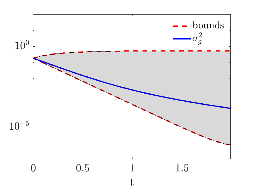
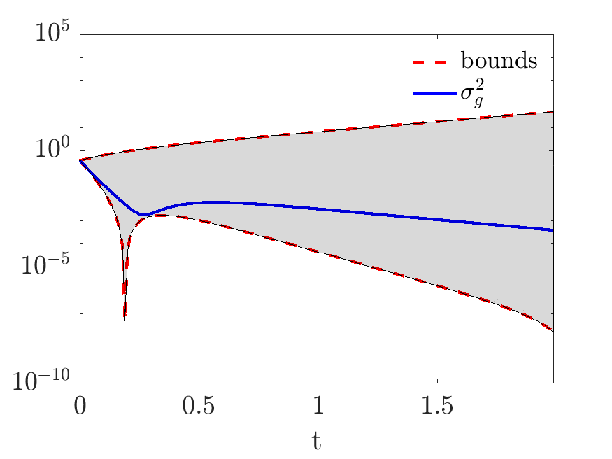
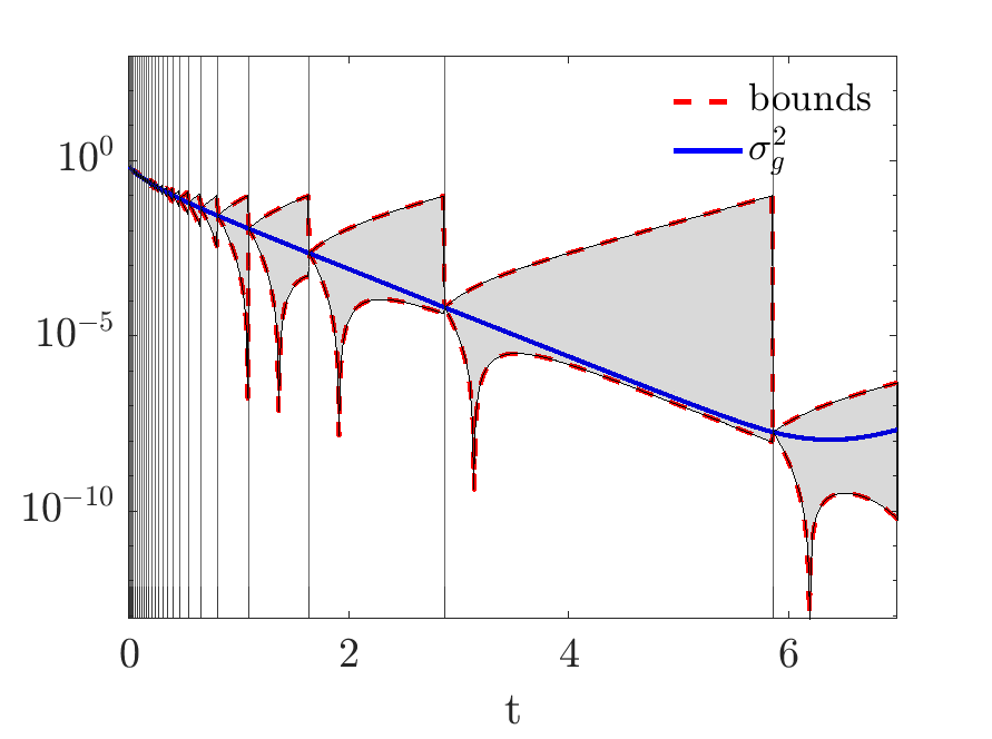
Figure 3.2 shows two examples for the decay of σ2[g]superscript𝜎2delimited-[]𝑔\sigma^{2}[g] and the bounds for the kernel

(3.19) P(v,w)=α+K(ς+|vw|2)γ,α,ς,γ0, and K,formulae-sequence𝑃𝑣𝑤𝛼𝐾superscript𝜍superscript𝑣𝑤2𝛾𝛼𝜍formulae-sequence𝛾0 and 𝐾P(v,w)=\alpha+\frac{K}{(\varsigma+|v-w|^{2})^{\gamma}},\qquad\alpha,\varsigma,\gamma\geq 0,\textrm{ and }K\in\mathbb{R}\,,

associated to Cucker-Smale consensus dynamics [27]. On the left, we consider the attractive case where P()𝑃P(\cdot) is positive and bounded in [0,1]01[0,1], with α=0,ς=1,K=1formulae-sequence𝛼0formulae-sequence𝜍1𝐾1\alpha=0,\varsigma=1,K=1 and γ=2𝛾2\gamma=2. On the right, we show an attraction-repulsion dynamics with kernel 1P(,)91𝑃9-1\leq P(\cdot,\cdot)\leq 9 where α=9,ς=0.1,K=1formulae-sequence𝛼9formulae-sequence𝜍0.1𝐾1\alpha=9,\varsigma=0.1,K=-1 and γ=1𝛾1\gamma=1. The value of σg2superscriptsubscript𝜎𝑔2\sigma_{g}^{2} is computed integrating numerically a mean-field approximation of the nonlinear dynamic equation. In both cases, the initial density of particle g0(v)superscript𝑔0𝑣g^{0}(v) is

g0(v)=23χ[1/4,7/4](v).superscript𝑔0𝑣23subscript𝜒1474𝑣g^{0}(v)=\frac{2}{3}\chi_{[1/4,7/4]}(v).

.

0P(v,w)10𝑃𝑣𝑤10\leq P(v,w)\leq 1 1P(v,w)91𝑃𝑣𝑤9-1\leq P(v,w)\leq 9
Refer to caption Refer to caption
Figure 3.2: Variance decay and bounds for the open-loop approach (2.25). On the left we observe the decay for an attractive dynamics, on the right the attractive-repulsive case.
Remark 3.4 (Bounds for inexact open-loop Riccati control).

For the inexact open-loop Riccati control we observe that bounds on moments can be computed in similar fashion. From (3.9), the first moment is given by

(3.20) ddtm1[g](t)=kd(t)+ko(t)νm1[g0],m1[g](0)=m1[g0].formulae-sequence𝑑𝑑𝑡subscript𝑚1delimited-[]𝑔𝑡subscript𝑘𝑑𝑡subscript𝑘𝑜𝑡𝜈subscript𝑚1delimited-[]superscript𝑔0subscript𝑚1delimited-[]𝑔0subscript𝑚1delimited-[]superscript𝑔0\frac{d}{dt}m_{1}[g](t)=-\frac{k_{d}(t)+k_{o}(t)}{\nu}m_{1}[g^{0}],\qquad m_{1}[g](0)=m_{1}[g^{0}].

A substantial difference with respect to the exponential decay of the average (3.10) is observed since the exact solution to (3.20) is

(3.21) m1[g](t)=m1[g0](11ν0t(kd(s)+ko(s))𝑑s).subscript𝑚1delimited-[]𝑔𝑡subscript𝑚1delimited-[]superscript𝑔011𝜈superscriptsubscript0𝑡subscript𝑘𝑑𝑠subscript𝑘𝑜𝑠differential-d𝑠m_{1}[g](t)=m_{1}[g^{0}]\left(1-\frac{1}{\nu}\int_{0}^{t}(k_{d}(s)+k_{o}(s))\ ds\right).

Bounds of the variance of g(v,t)𝑔𝑣𝑡g(v,t) are retrieved as a particular case of Proposition 2. The time evolution of σ2[g]superscript𝜎2delimited-[]𝑔\sigma^{2}[g] reads

(3.22) ddtσ2[g]=2d|vv|2P(v,v)gg𝑑v𝑑v2kdνϱ[g0,g]σ2[g0]σ2[g],𝑑𝑑𝑡superscript𝜎2delimited-[]𝑔subscriptsuperscript2𝑑superscript𝑣subscript𝑣2𝑃𝑣subscript𝑣𝑔subscript𝑔differential-d𝑣differential-dsubscript𝑣2subscript𝑘𝑑𝜈italic-ϱsuperscript𝑔0𝑔superscript𝜎2delimited-[]superscript𝑔0superscript𝜎2delimited-[]𝑔\frac{d}{dt}\sigma^{2}[g]=-\int_{\mathbb{R}^{2d}}\!\!\!\!\!|v-v_{*}|^{2}P(v,v_{*})gg_{*}dvdv_{*}-2\frac{k_{d}}{\nu}\varrho[g^{0},g]\sqrt{\sigma^{2}[g^{0}]\sigma^{2}[g]},

and the bounds for σ2[g](t)superscript𝜎2delimited-[]𝑔𝑡\sigma^{2}[g](t) correspond to the estimate in (3.14) with β(t)1𝛽𝑡1\beta(t)\equiv 1,

(3.23) σ2[g0]e2bt(11ν0tebskd(s)𝑑s)2σ2[g](t)σ2[g0]e2at(1+1ν0teaskd(s)𝑑s)2superscript𝜎2delimited-[]superscript𝑔0superscript𝑒2𝑏𝑡superscript11𝜈superscriptsubscript0𝑡superscript𝑒𝑏𝑠subscript𝑘𝑑𝑠differential-d𝑠2superscript𝜎2delimited-[]𝑔𝑡superscript𝜎2delimited-[]superscript𝑔0superscript𝑒2𝑎𝑡superscript11𝜈superscriptsubscript0𝑡superscript𝑒𝑎𝑠subscript𝑘𝑑𝑠differential-d𝑠2\sigma^{2}[g^{0}]e^{-2bt}\left(1-\frac{1}{\nu}\int_{0}^{t}e^{bs}k_{d}(s)\!\ ds\right)^{2}\!\!\!\leq\sigma^{2}[g](t)\leq\sigma^{2}[g^{0}]e^{2at}\left(1+\frac{1}{\nu}\int_{0}^{t}e^{-as}k_{d}(s)\!\ ds\right)^{2}

The loss of the exponential decay of the average (3.10) constitutes the main drawback of this approach, although we can still steer the density towards a reference solution.

3.2 Closed-loop Riccati control

We perform the derivation of the mean-field limit and moment bounds for the system (2.23). Given the mean-field density g(v,t)𝑔𝑣𝑡g(v,t), the mean-field limit of (2.23) is

(3.24) tg=v(g(𝒫[g]kdνvkoνm1[g])),g(v,0)=g0(v),formulae-sequencesubscript𝑡𝑔subscript𝑣𝑔𝒫delimited-[]𝑔subscript𝑘𝑑𝜈𝑣subscript𝑘𝑜𝜈subscript𝑚1delimited-[]𝑔𝑔𝑣0superscript𝑔0𝑣\partial_{t}g=-\nabla_{v}\cdot\left(g\left(\mathcal{P}[g]-\frac{k_{d}}{\nu}v-\frac{k_{o}}{\nu}m_{1}[g]\right)\right),\qquad\qquad\,\,g(v,0)=g^{0}(v)\,,

where ko(t),kd(t)subscript𝑘𝑜𝑡subscript𝑘𝑑𝑡k_{o}(t),k_{d}(t) are obtained by a Riccati system (3.4).

3.2.1 Bounds of decay moments

The first moment and variance equations are given in the following Lemma.

Lemma 3.

Under the assumption (A) the first moment of (3.24) evolves according (3.10). The evolution of the variance σ2[g]superscript𝜎2delimited-[]𝑔\sigma^{2}[g] satisfies the equation

(3.25) ddtσ2[g]=|vv|2P(v,v)g(v)g(v)𝑑v𝑑v2kdνσ2[g].𝑑𝑑𝑡superscript𝜎2delimited-[]𝑔double-integralsuperscript𝑣subscript𝑣2𝑃𝑣subscript𝑣𝑔𝑣𝑔subscript𝑣differential-d𝑣differential-dsubscript𝑣2subscript𝑘𝑑𝜈superscript𝜎2delimited-[]𝑔\frac{d}{dt}{\sigma}^{2}[g]=-\iint|v-v_{*}|^{2}P(v,v_{*})g(v)g(v_{*})dvdv_{*}-\frac{2k_{d}}{\nu}\sigma^{2}[g].

We omit the computations of the proof, since they follow the same line of Lemma 1. In particular, it is enough to observe that the variance equation of the open-loop Riccati (3.11) collapses to (3.25) taking f(t,v)=g(t,v)𝑓𝑡𝑣𝑔𝑡𝑣f(t,v)=g(t,v). The following estimates on the decay of the variance hold.

Proposition 4.

Under assumption (A) on the interaction kernel P()𝑃P(\cdot), there exist lower and upper bounds for the variance of g𝑔g given by

(3.26) σ2[g0]e2btCν(0,t)σ2[g](t)σ2[g0]e2atCν(0,t).superscript𝜎2delimited-[]superscript𝑔0superscript𝑒2𝑏𝑡subscript𝐶𝜈0𝑡superscript𝜎2delimited-[]𝑔𝑡superscript𝜎2delimited-[]superscript𝑔0superscript𝑒2𝑎𝑡subscript𝐶𝜈0𝑡\sigma^{2}[g^{0}]e^{-2bt}C_{\nu}(0,t)\leq\sigma^{2}[g](t)\leq\sigma^{2}[g^{0}]e^{2at}C_{\nu}(0,t).

where

Cν(0,t)=exp{2ν0tkd(s)𝑑s}.subscript𝐶𝜈0𝑡2𝜈superscriptsubscript0𝑡subscript𝑘𝑑𝑠differential-d𝑠C_{\nu}(0,t)=\exp\left\{-\frac{2}{\nu}\int_{0}^{t}k_{d}(s)ds\right\}.

Proof 3.5.

Since the interaction kernel is bounded and using the identity (3.13) for σ2[g]superscript𝜎2delimited-[]𝑔\sigma^{2}[g], it follows that

(3.27) 2(b+kdν)σ2[g]ddtσ2[g]2(akdν)σ2[g].2𝑏subscript𝑘𝑑𝜈superscript𝜎2delimited-[]𝑔𝑑𝑑𝑡superscript𝜎2delimited-[]𝑔2𝑎subscript𝑘𝑑𝜈superscript𝜎2delimited-[]𝑔-2\Big{(}b+\frac{k_{d}}{\nu}\Big{)}\sigma^{2}[g]\leq\frac{d}{dt}{\sigma}^{2}[g]\leq 2\Big{(}a-\frac{k_{d}}{\nu}\Big{)}\sigma^{2}[g].

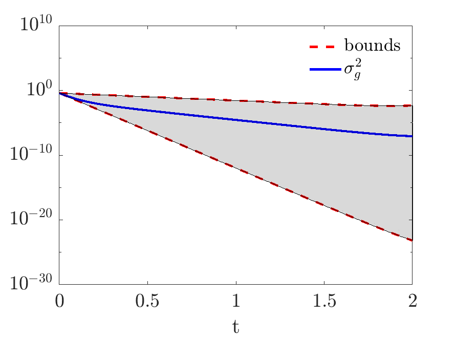
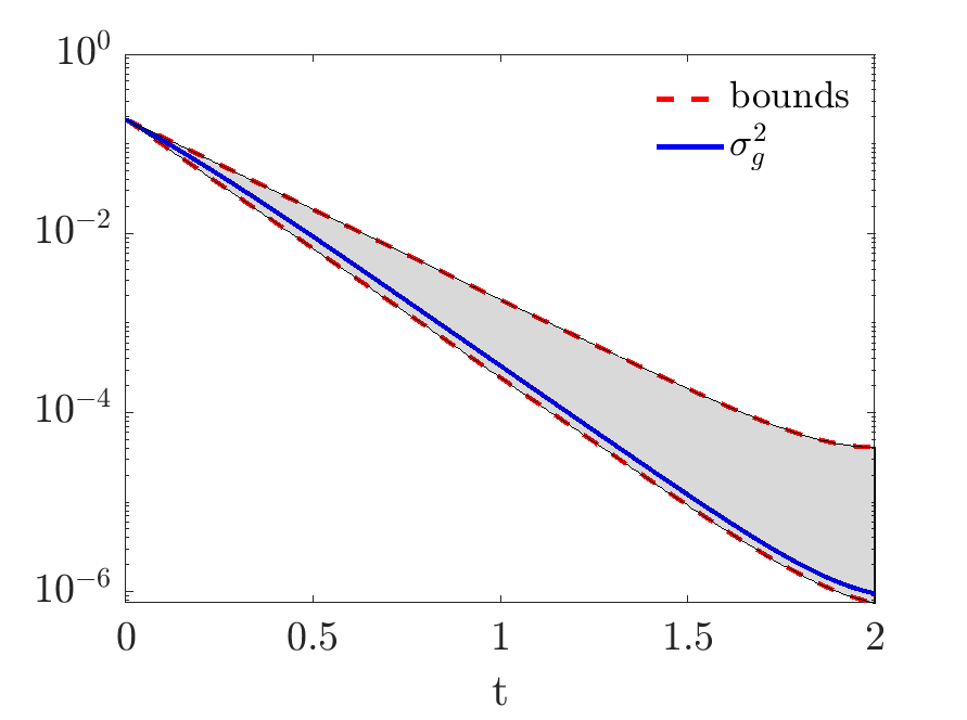
In Figure 3.3 the decay of the variance σ2[g]superscript𝜎2delimited-[]𝑔\sigma^{2}[g] and the bounds associated to kernel (3.19) are shown. We choose the same parameters as reported in Figure 3.2. We observe that bounds of the closed-loop control (2.23) are closer compared to equation (2.25). Moreover, a stronger decay is observed. Hence, we expect a better performance of the closed-loop control over the open-loop approaches. However, the open-loop approach (2.25) is useful when dealing with incomplete information or limited access to the non-linear dynamics.

We devote the next section to the development of a synthesis method based on predictive horizons estimated a-priori through the bounds of the open-loop strategy (2.25).
0P(v,w)10𝑃𝑣𝑤10\leq P(v,w)\leq 1 1P(v,w)91𝑃𝑣𝑤9-1\leq P(v,w)\leq 9
Refer to caption Refer to caption
Figure 3.3: Variance decay and bounds for the open-loop approach (2.23). On the left we observe the decay for an attractive dynamics, on the right the attractive-repulsive case.

4 Moment-driven predictive control (MdPC)

In order to utilize the stabilization properties of the control loops proposed in the previous sections, we discuss their implementation in a receding horizon framework. Here, we prescribe a control horizon where the control signal is applied, after which there is an update procedure including a re-calculation of the control law based on the current state of the system. There exists a vast literature addressing the design of nonlinear model predictive control (MPC) algorithms, we refer the reader to [54, 45] and references therein.

In the general nonlinear MPC control algorithm, an open-loop optimal control signal is synthesized over a prediction horizon [0,Tp]0subscript𝑇𝑝[0,T_{p}], by solving a problem of the form (2.1). Having prescribed the system dynamics and the running cost, this optimization problem depends on the initial state v(0)𝑣0v(0) and the horizon Tpsubscript𝑇𝑝T_{p} only. The optimal signal usuperscript𝑢u^{*}, which is obtained for the whole horizon [0,Tp]0subscript𝑇𝑝[0,T_{p}], is implemented over a shorter control horizon [0,Tc]0subscript𝑇𝑐[0,T_{c}]. At t=Tc𝑡subscript𝑇𝑐t=T_{c} the initial state of the system is re-calibrated to v(0)=v(Tc)𝑣0𝑣subscript𝑇𝑐v(0)=v(T_{c}) and the optimization is repeated. Relevant issues in the MPC literature are the selection of suitable horizons Tpsubscript𝑇𝑝T_{p} and Tcsubscript𝑇𝑐T_{c} which can ensure asymptotic stability of the closed-loop, as well as the design of effective optimization methods to make this implementation suitable for real-time control.

Here instead, we propose a novel class of MPC-type algorithms where instead of fixing a prediction horizon, the re-calibration of the control laws (2.25)-(2.26) is triggered adaptively in time based on a direct estimate of the moments decay. This is similar in spirit to the literature on event-based MPC methods, see for example [36] where an event-based framework for the control of a team of cooperating distributed agents and [65] for networked systems is proposed.

Variance driven Predictive Control MdPC(σ2superscript𝜎2\sigma^{2})

Starting from the open-loop control (3.6) we consider densities at initial time given by g(v,0)=g0(v)𝑔𝑣0superscript𝑔0𝑣g(v,0)=g^{0}(v), f0(w)g0(w)superscript𝑓0𝑤superscript𝑔0𝑤f^{0}(w)\equiv g^{0}(w) and the joint distribution λ0(v,w)λ(v,w,t0)superscript𝜆0𝑣𝑤𝜆𝑣𝑤subscript𝑡0\lambda^{0}(v,w)\equiv\lambda(v,w,t_{0}). To shorten the notation we introduce the general semi-discretization of the mean-field dynamics (3.5) as follows

(4.1) λn+1(v,w)=ΦΔt[λn;un[fn]](v,w),λ0(v,w)=λ(v,w,0),n0,formulae-sequencesuperscript𝜆𝑛1𝑣𝑤subscriptΦΔ𝑡superscript𝜆𝑛superscript𝑢𝑛delimited-[]superscript𝑓𝑛𝑣𝑤formulae-sequencesuperscript𝜆0𝑣𝑤𝜆𝑣𝑤0𝑛0\lambda^{n+1}(v,w)=\Phi_{\Delta t}[\lambda^{n};u^{n}[f^{n}]](v,w),\qquad\lambda^{0}(v,w)=\lambda(v,w,0),\quad n\geq 0,

coupled with the solution of the Riccati system (3.4). Here, ΦΔtsubscriptΦΔ𝑡\Phi_{\Delta t} defines the time discretization, and un[fn]superscript𝑢𝑛delimited-[]superscript𝑓𝑛u^{n}[f^{n}] encodes the control dependency on the density, given by

(4.2) un[fn](w,tn)=1ν(kd(tn)w+ko(tn)m1[fn](tn)).superscript𝑢𝑛delimited-[]superscript𝑓𝑛𝑤subscript𝑡𝑛1𝜈subscript𝑘𝑑subscript𝑡𝑛𝑤subscript𝑘𝑜subscript𝑡𝑛subscript𝑚1delimited-[]superscript𝑓𝑛subscript𝑡𝑛u^{n}[f^{n}](w,t_{n})=\frac{1}{\nu}\left(k_{d}(t_{n})w+k_{o}(t_{n})m_{1}[f^{n}](t_{n})\right).

Our goal is to predict the error in the variance decay σ2[g](t)superscript𝜎2delimited-[]𝑔𝑡\sigma^{2}[g](t) directly from (3.14) by computing the difference between the upper and lower bounds

(4.3) Δσ(t0,t)=σ2[g(v,t0)][(e2a(tt0)(1+Ba(t0,t))2e2b(tt0)(1Bb+(t0,t))2],\Delta_{\sigma}(t_{0},t)=\sigma^{2}[g(v,t_{0})]\left[(e^{2a(t-t_{0})}\left(1+B^{-}_{a}(t_{0},t)\right)^{2}-e^{-2b(t-t_{0})}\left(1-B^{+}_{b}(t_{0},t)\right)^{2}\right],

where Bc±(t0,t)subscriptsuperscript𝐵plus-or-minus𝑐subscript𝑡0𝑡B^{\pm}_{c}(t_{0},t) are the quantities defined in (3.15). Then we can use Δσ(t0,t)subscriptΔ𝜎subscript𝑡0𝑡\Delta_{\sigma}(t_{0},t) to control the decay of the variance σ2[g](t)superscript𝜎2delimited-[]𝑔𝑡\sigma^{2}[g](t) in order to keep the variance of g(v,t)𝑔𝑣𝑡g(v,t) below a fixed threshold δ>0𝛿0\delta>0. In this way, we can find time t1>t0subscript𝑡1subscript𝑡0t_{1}>t_{0} such that Δσ(t0,t1)>δsubscriptΔ𝜎subscript𝑡0subscript𝑡1𝛿\Delta_{\sigma}(t_{0},t_{1})>\delta and evolve the dynamics in the time interval [t0,t1]subscript𝑡0subscript𝑡1[t_{0},t_{1}]. The procedure is reinitialized updating the state of the linearized dynamics at time t1subscript𝑡1t_{1} by setting f(t1,v)g(t1,v)𝑓subscript𝑡1𝑣𝑔subscript𝑡1𝑣f(t_{1},v)\equiv g(t_{1},v). We formalize this procedure in Algorithm 1.

Algorithm 1 [MdPC(σ2superscript𝜎2\sigma^{2})]
  0. Set k0𝑘0k\leftarrow 0, tk=0subscript𝑡𝑘0t_{k}=0, gk(v)=g(v,0)superscript𝑔𝑘𝑣𝑔𝑣0g^{k}(v)=g(v,0), fk(v)=g(v,0)superscript𝑓𝑘𝑣𝑔𝑣0f^{k}(v)=g(v,0) and tolerance δ𝛿\delta
  1. Solve the Riccati equation to obtain kdsubscript𝑘𝑑k_{d}, kosubscript𝑘𝑜k_{o} on the time interval [0,T]0𝑇[0,T]
  2. Find the time tk+1subscript𝑡𝑘1t_{k+1} such that tk+1:=min{t|tk<tT,Δσ(tk,t)>δ}assignsubscript𝑡𝑘1conditional𝑡subscript𝑡𝑘𝑡𝑇subscriptΔ𝜎subscript𝑡𝑘𝑡𝛿t_{k+1}:=\min\{t|t_{k}<t\leq T,\Delta_{\sigma}(t_{k},t)>\delta\}
  while tk+1Tsubscript𝑡𝑘1𝑇t_{k+1}\leq T do
     i. Evolve the dynamics (4.1) up to tk+1subscript𝑡𝑘1t_{k+1}
     ii. Set gk+1(v)=g(v,tk+1)subscript𝑔𝑘1𝑣𝑔𝑣subscript𝑡𝑘1g_{k+1}(v)=g(v,t_{k+1}), fk+1(v)=g(v,tk+1)subscript𝑓𝑘1𝑣𝑔𝑣subscript𝑡𝑘1f_{k+1}(v)=g(v,t_{k+1})
     iii. kk+1𝑘𝑘1k\leftarrow k+1
     iv. Compute tk+1subscript𝑡𝑘1t_{k+1} from step 2. 
  end while
Mean and variance driven predictive control, MdPC(m1,σ2)MdPCsubscript𝑚1superscript𝜎2\textrm{MdPC}(m_{1},\sigma^{2})

For the inexact open-loop control approach (3.9) it is necessary to modify the previous algorithm controlling also the decay of the first moment of g=g(v,t)𝑔𝑔𝑣𝑡g=g(v,t). For this, we introduce the semidiscretized mean-field model of (3.9)

(4.4) λn+1(v,w)superscript𝜆𝑛1𝑣𝑤\displaystyle\lambda^{n+1}(v,w) =ΦΔt[λn;un[g0]](v,w),λ0(v,w)=λ(v,w,0),n0,formulae-sequenceabsentsubscriptΦΔ𝑡superscript𝜆𝑛superscript𝑢𝑛delimited-[]superscript𝑔0𝑣𝑤formulae-sequencesuperscript𝜆0𝑣𝑤𝜆𝑣𝑤0𝑛0\displaystyle=\Phi_{\Delta t}[\lambda^{n};u^{n}[g^{0}]](v,w),\qquad\lambda^{0}(v,w)=\lambda(v,w,0),\quad n\geq 0\,,

where the control is given by

(4.5) un[g0](w,tn)=1ν(kd(tn)w+ko(tn)m1[g0]).superscript𝑢𝑛delimited-[]superscript𝑔0𝑤subscript𝑡𝑛1𝜈subscript𝑘𝑑subscript𝑡𝑛𝑤subscript𝑘𝑜subscript𝑡𝑛subscript𝑚1delimited-[]superscript𝑔0u^{n}[g^{0}](w,t_{n})=\frac{1}{\nu}\left(k_{d}(t_{n})w+k_{o}(t_{n})m_{1}[g^{0}]\right).

According to the bounds (3.23), the decay of the variance is controlled by Δσ(t0,t)subscriptΔ𝜎subscript𝑡0𝑡\Delta_{\sigma}(t_{0},t) as in (4.3) with

(4.6) Bc±(t0,t)=1νt0tt0kd(s)e±c(st0)𝑑s.subscriptsuperscript𝐵plus-or-minus𝑐subscript𝑡0𝑡1𝜈superscriptsubscriptsubscript𝑡0𝑡subscript𝑡0subscript𝑘𝑑𝑠superscript𝑒plus-or-minus𝑐𝑠subscript𝑡0differential-d𝑠B^{\pm}_{c}(t_{0},t)=\frac{1}{\nu}\int_{t_{0}}^{t-t_{0}}k_{d}(s)e^{\pm c(s-t_{0})}ds.

However, in this case the convergence towards the desired state is not guaranteed since the decay of the first moment (3.21) does not match the moment of the linearized model (3.6b). To guarantee consensus convergence we require (3.21) to be contractive. For this, we introduce the control quantity

(4.7) Δm(t0,t)=|11νt0tt0(kd(s)+ko(s))𝑑s|,0<τ1,formulae-sequencesubscriptΔ𝑚subscript𝑡0𝑡11𝜈superscriptsubscriptsubscript𝑡0𝑡subscript𝑡0subscript𝑘𝑑𝑠subscript𝑘𝑜𝑠differential-d𝑠0𝜏1\Delta_{m}(t_{0},t)=\left|1-\frac{1}{\nu}\int_{t_{0}}^{t-t_{0}}(k_{d}(s)+k_{o}(s))\ ds\right|,\qquad 0<\tau\leq 1\,,

which we use to determine updates in Algorithm 2.

Algorithm 2 [MdPC(m1,σ2)subscript𝑚1superscript𝜎2(m_{1},\sigma^{2})]
  0. Set k0𝑘0k\leftarrow 0, tk=0subscript𝑡𝑘0t_{k}=0, gk(v)=g(v,0)superscript𝑔𝑘𝑣𝑔𝑣0g^{k}(v)=g(v,0) and tolerances δ,τ>0𝛿𝜏0\delta,\tau>0
  1. Solve the Riccati equation to obtain kdsubscript𝑘𝑑k_{d}, kosubscript𝑘𝑜k_{o} on the time interval [0,T]0𝑇[0,T]. 
  2. Find the times tδ,tτsubscript𝑡𝛿subscript𝑡𝜏t_{\delta},t_{\tau} such
(4.8) tδsubscript𝑡𝛿\displaystyle t_{\delta} :=min{t|tk<tT,Δσ(tk,t)>δ},assignabsentconditional𝑡subscript𝑡𝑘𝑡𝑇subscriptΔ𝜎subscript𝑡𝑘𝑡𝛿\displaystyle:=\min\{t|t_{k}<t\leq T,\Delta_{\sigma}(t_{k},t)>\delta\},
tτsubscript𝑡𝜏\displaystyle t_{\tau} :=min{t|tk<tT,Δm(tk,t)>τ},assignabsentconditional𝑡subscript𝑡𝑘𝑡𝑇subscriptΔ𝑚subscript𝑡𝑘𝑡𝜏\displaystyle:=\min\{t|t_{k}<t\leq T,\Delta_{m}(t_{k},t)>\tau\},
tk+1subscript𝑡𝑘1\displaystyle t_{k+1} :=min{tδ,tτ}assignabsentsubscript𝑡𝛿subscript𝑡𝜏\displaystyle:=\min\left\{t_{\delta},t_{\tau}\right\}
  while tk+1Tsubscript𝑡𝑘1𝑇t_{k+1}\leq T do
     i. Evolve the dynamics (4.4) up to tk+1subscript𝑡𝑘1t_{k+1}
     ii. Set gk+1(v)=g(v,tk+1)superscript𝑔𝑘1𝑣𝑔𝑣subscript𝑡𝑘1g^{k+1}(v)=g(v,t_{k+1}) and g0(v)=g(v,tk+1)superscript𝑔0𝑣𝑔𝑣subscript𝑡𝑘1g^{0}(v)=g(v,t_{k+1})
     iii. kk+1𝑘𝑘1k\leftarrow k+1
     iv. Compute tk+1subscript𝑡𝑘1t_{k+1} from (4.8);
  end while
Remark 4.1.

We observe that when an update is performed at each time step, that is for values of δ𝛿\delta small enough, the MdPC approaches is equivalent to a discretization of the closed-loop control (3.24). Indeed, since for every n0,𝑛0n\geq 0, we have fngnsuperscript𝑓𝑛superscript𝑔𝑛f^{n}\equiv g^{n} , the mean-field model (4.1) reduces to

(4.9) gn+1(v)superscript𝑔𝑛1𝑣\displaystyle g^{n+1}(v) =ΦΔt[gn;u[gn]](v),n0,g0(v)=g(v,t0),formulae-sequenceabsentsubscriptΦΔ𝑡superscript𝑔𝑛𝑢delimited-[]superscript𝑔𝑛𝑣formulae-sequence𝑛0superscript𝑔0𝑣𝑔𝑣subscript𝑡0\displaystyle=\Phi_{\Delta t}[g^{n};u[g^{n}]](v),\qquad n\geq 0,\qquad g^{0}(v)=g(v,t_{0}),

where the control is given by u[gn](v,tn)=1ν(kd(tn)v+ko(tn)m1[gn](tn))𝑢delimited-[]superscript𝑔𝑛𝑣subscript𝑡𝑛1𝜈subscript𝑘𝑑subscript𝑡𝑛𝑣subscript𝑘𝑜subscript𝑡𝑛subscript𝑚1delimited-[]superscript𝑔𝑛subscript𝑡𝑛u[g^{n}](v,t_{n})=\frac{1}{\nu}\left(k_{d}(t_{n})v+k_{o}(t_{n})m_{1}[g^{n}](t_{n})\right) .

5 Numerical Experiments

In this section we present different numerical tests on microscopic and mean-field dynamics. We analyze three different cases: a first-order opinion dynamics, a second-order alignment model, and first-order aggregation model. For the numerical solution of the mean-field model (3.6) we employ mean-field Monte-Carlo methods (MFMCs) developed in [7]. These methods fall in the class of fast algorithms developed for interacting particle systems such as direct simulation Monte-Carlo methods (DSMCs) [15, 32, 11], or most recently Random Batch Methods (RBMs) [55].

We consider Nssubscript𝑁𝑠N_{s} particles v0{vi0}isuperscript𝑣0subscriptsuperscriptsubscript𝑣𝑖0𝑖v^{0}\equiv\left\{v_{i}^{0}\right\}_{i} sampled from the initial distribution g0(v)superscript𝑔0𝑣g^{0}(v), and we duplicate the sample defining w0v0superscript𝑤0superscript𝑣0w^{0}\equiv v^{0} for the linearized dynamics. We introduce the following approximation for the mean-field dynamics

(5.1a) vin+1superscriptsubscript𝑣𝑖𝑛1\displaystyle v_{i}^{n+1} =(1ΔtP^in)vin+ΔtP^inV^inΔtuin,absent1Δ𝑡superscriptsubscript^𝑃𝑖𝑛superscriptsubscript𝑣𝑖𝑛Δ𝑡superscriptsubscript^𝑃𝑖𝑛subscriptsuperscript^𝑉𝑛𝑖Δ𝑡superscriptsubscript𝑢𝑖𝑛\displaystyle=(1-\Delta t\hat{P}_{i}^{n})v_{i}^{n}+\Delta t\hat{P}_{i}^{n}\hat{V}^{n}_{i}-\Delta tu_{i}^{n},
(5.1b) win+1superscriptsubscript𝑤𝑖𝑛1\displaystyle w_{i}^{n+1} =(1Δtp¯)win+Δtp¯m^1nΔtuin,absent1Δ𝑡¯𝑝superscriptsubscript𝑤𝑖𝑛Δ𝑡¯𝑝superscriptsubscript^𝑚1𝑛Δ𝑡superscriptsubscript𝑢𝑖𝑛\displaystyle=(1-\Delta t\bar{p})w_{i}^{n}+\Delta t\bar{p}\hat{m}_{1}^{n}-\Delta tu_{i}^{n},

for n0𝑛0n\geq 0 and where the quantities P^insuperscriptsubscript^𝑃𝑖𝑛\hat{P}_{i}^{n} and V^insubscriptsuperscript^𝑉𝑛𝑖\hat{V}^{n}_{i} are computed from a sub-sample of M𝑀M particles randomly selected from the whole ensemble of Nssubscript𝑁𝑠N_{s} particles as follows

P^in=1Mk=1MP(vin,vikn),V^in=1Mk=1MP(vin,vikn)P^invikn,i=1,,Ns.formulae-sequencesubscriptsuperscript^𝑃𝑛𝑖1𝑀superscriptsubscript𝑘1𝑀𝑃subscriptsuperscript𝑣𝑛𝑖subscriptsuperscript𝑣𝑛subscript𝑖𝑘formulae-sequencesubscriptsuperscript^𝑉𝑛𝑖1𝑀superscriptsubscript𝑘1𝑀𝑃subscriptsuperscript𝑣𝑛𝑖subscriptsuperscript𝑣𝑛subscript𝑖𝑘subscriptsuperscript^𝑃𝑛𝑖subscriptsuperscript𝑣𝑛subscript𝑖𝑘𝑖1subscript𝑁𝑠\hat{P}^{n}_{i}=\frac{1}{M}\sum_{k=1}^{M}P(v^{n}_{i},v^{n}_{i_{k}}),\qquad\hat{V}^{n}_{i}=\frac{1}{M}\sum_{k=1}^{M}\frac{P(v^{n}_{i},v^{n}_{i_{k}})}{\hat{P}^{n}_{i}}v^{n}_{i_{k}},\qquad i=1,\ldots,N_{s}.

For the open-loop mean-field dynamics (4.1) the control uinsubscriptsuperscript𝑢𝑛𝑖u^{n}_{i} is defined as

(5.2) uin=1ν(kdnwin+konm^1n),m^1n=1Nsj=1Nswin.formulae-sequencesuperscriptsubscript𝑢𝑖𝑛1𝜈superscriptsubscript𝑘𝑑𝑛superscriptsubscript𝑤𝑖𝑛superscriptsubscript𝑘𝑜𝑛superscriptsubscript^𝑚1𝑛superscriptsubscript^𝑚1𝑛1subscript𝑁𝑠superscriptsubscript𝑗1subscript𝑁𝑠superscriptsubscript𝑤𝑖𝑛u_{i}^{n}=-\frac{1}{\nu}\left(k_{d}^{n}w_{i}^{n}+k_{o}^{n}\hat{m}_{1}^{n}\right),\qquad\hat{m}_{1}^{n}=\frac{1}{N_{s}}\sum_{j=1}^{N_{s}}w_{i}^{n}.

The scheme (5.1) reduces to a set of equations for the mean-field dynamics for the closed-loop (4.9) and inexact open-loop (4.4), respectively. In the closed-loop setting (4.9) the control term is computed as

(5.3) uin=1ν(kdnvin+konm^1n),m^1n=1Nsj=1Nsvin,formulae-sequencesuperscriptsubscript𝑢𝑖𝑛1𝜈superscriptsubscript𝑘𝑑𝑛superscriptsubscript𝑣𝑖𝑛superscriptsubscript𝑘𝑜𝑛superscriptsubscript^𝑚1𝑛superscriptsubscript^𝑚1𝑛1subscript𝑁𝑠superscriptsubscript𝑗1subscript𝑁𝑠superscriptsubscript𝑣𝑖𝑛u_{i}^{n}=-\frac{1}{\nu}\left(k_{d}^{n}v_{i}^{n}+k_{o}^{n}\hat{m}_{1}^{n}\right),\qquad\hat{m}_{1}^{n}=\frac{1}{N_{s}}\sum_{j=1}^{N_{s}}v_{i}^{n},

and in the inexact open-loop approach (4.4) we have

(5.4) uin=1ν(kdnvi0+konm^10),m^10=1Nsj=1Nsvi0.formulae-sequencesuperscriptsubscript𝑢𝑖𝑛1𝜈superscriptsubscript𝑘𝑑𝑛superscriptsubscript𝑣𝑖0superscriptsubscript𝑘𝑜𝑛superscriptsubscript^𝑚10superscriptsubscript^𝑚101subscript𝑁𝑠superscriptsubscript𝑗1subscript𝑁𝑠superscriptsubscript𝑣𝑖0u_{i}^{n}=-\frac{1}{\nu}\left(k_{d}^{n}v_{i}^{0}+k_{o}^{n}\hat{m}_{1}^{0}\right),\qquad\hat{m}_{1}^{0}=\frac{1}{N_{s}}\sum_{j=1}^{N_{s}}v_{i}^{0}.

We report in Table 5.1 the different choices of parameters used for the numerical discretization of the mean-field dynamics and for each control approach, respectively. We compare the performance of the control laws through the discretized cost

(5.5) JΔt,Ns(u,g0):=ΔtNsn=0NTj=1Ns(|vjn|2+ν|ujn|2),assignsubscript𝐽Δ𝑡subscript𝑁𝑠𝑢superscript𝑔0Δ𝑡subscript𝑁𝑠superscriptsubscript𝑛0subscript𝑁𝑇superscriptsubscript𝑗1subscript𝑁𝑠superscriptsubscriptsuperscript𝑣𝑛𝑗2𝜈superscriptsuperscriptsubscript𝑢𝑗𝑛2J_{\Delta t,N_{s}}(u,g^{0}):=\frac{\Delta t}{N_{s}}\sum_{n=0}^{N_{T}}\sum_{j=1}^{N_{s}}(|v^{n}_{j}|^{2}+\nu|u_{j}^{n}|^{2}),

with time step ΔtΔ𝑡\Delta t and Nssubscript𝑁𝑠N_{s} Monte Carlo samples.

Nssubscript𝑁𝑠N_{s} M ΔtΔ𝑡\Delta t ν𝜈\nu T𝑇T δ𝛿\delta τ𝜏\tau
Test 1: Opinion formation 1e4 100 1e-2 1e-2 111 1e-1 1
Test 2: Cucker-Smale dynamics 1e5 100 5e-2 1e-1 333 1
Test 3: Aggregation dynamics 1e5 10 1e-2 1 777 1e-1
Table 5.1: Simulation and optimization parameters for each test case.

5.1 Test 1: Opinion formation

We show an example in the context of opinion formation by Hegselmann and Krause [48]. We consider the positive interaction kernel defined as P(v,w)=Cχ(|wv|<η)𝑃𝑣𝑤𝐶𝜒𝑤𝑣𝜂P(v,w)=C\cdot\chi(|w-v|<\eta), where η=0.25𝜂0.25\eta=0.25 represents the confidence level and with a constant C=10𝐶10C=10, and χ𝜒\chi is an indicator function. The initial density of particle g0(v)superscript𝑔0𝑣g^{0}(v) is chosen such that consensus towards the target v¯=0¯𝑣0\bar{v}=0 would not be reached without control action, e.g. g0(v)=23χ[1/4,7/4](v)superscript𝑔0𝑣23subscript𝜒1474𝑣g^{0}(v)=\frac{2}{3}\chi_{[1/4,7/4]}(v) . We use the forward scheme (5.1) with fixed time step Δt=0.01Δ𝑡0.01\Delta t=0.01, sampling size Ns=10000subscript𝑁𝑠10000N_{s}=10000 of the initial distribution g0(v)superscript𝑔0𝑣g^{0}(v) and fixed M=100𝑀100M=100 for the approximation of the non-local interactions. To compare the mean-field dynamics with the microscopic we simulate N=50𝑁50N=50 agents uniformly sampled from g0superscript𝑔0g^{0}.

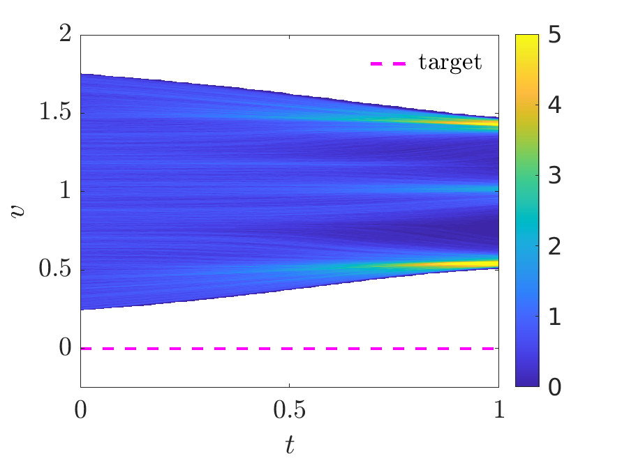
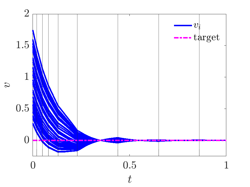
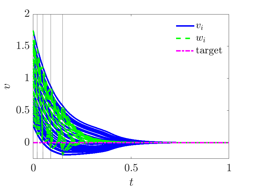
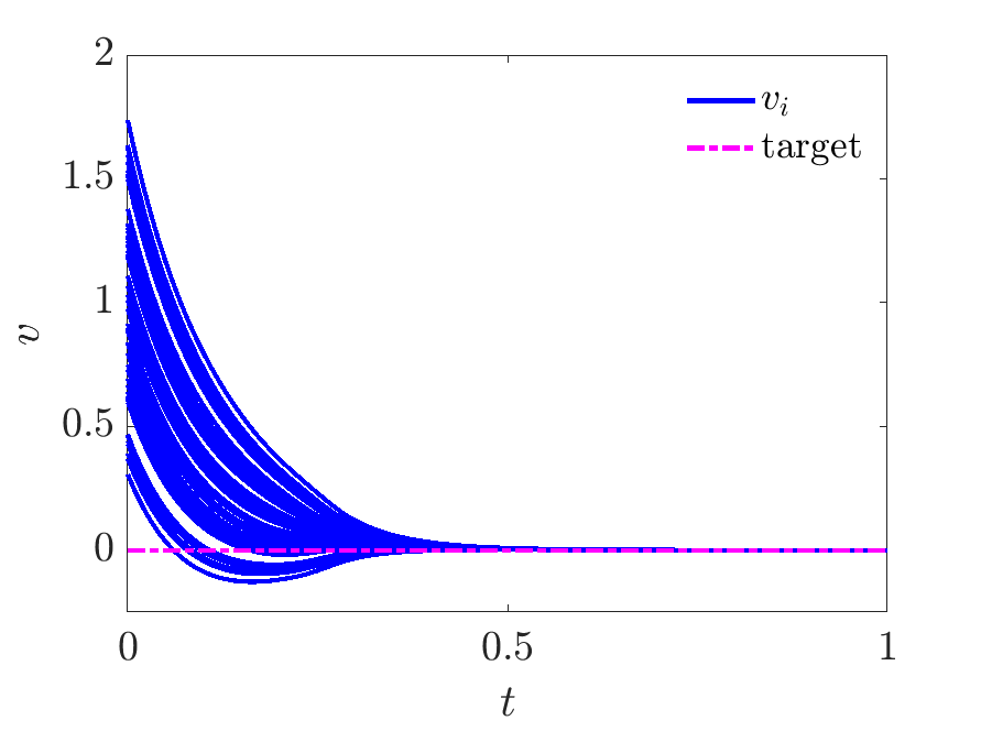
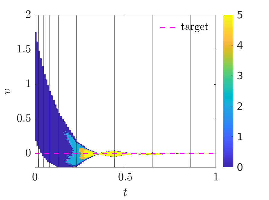
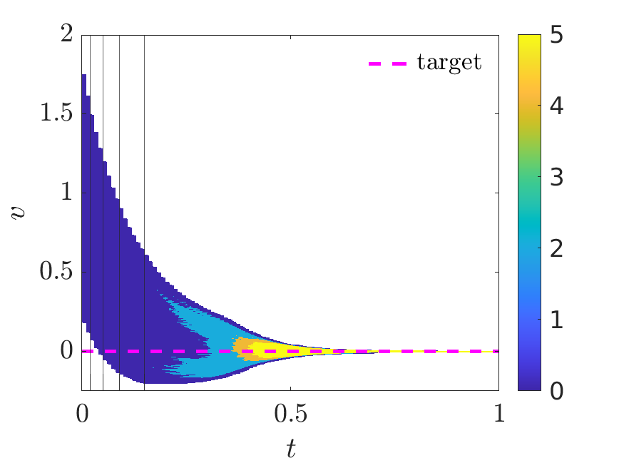
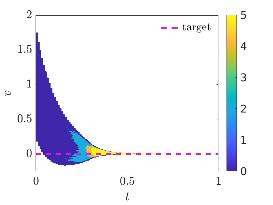
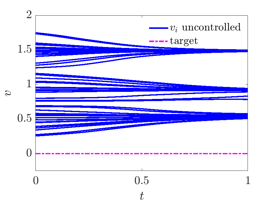
In the top row of Figure 5.4 the uncontrolled dynamics are shown, where clusters of opinions emerge due to structure of the interaction kernel P𝑃P. The second and third rows of Figure 5.4 depict the controlled dynamics for the microscopic and the mean-field dynamics. The left column of Figure 5.4 illustrates the convergence to the target when the MdPC(m1,σ2)subscript𝑚1superscript𝜎2(m_{1},\sigma^{2}) is applied. Algorithm 2 is used with δ𝛿\delta and τ𝜏\tau chosen according to Table (5.1). The vertical lines in the plots represent the times of the update. We have a different situation with the MdPC(σ2)superscript𝜎2(\sigma^{2}) approach 1, depicted in the middle column of Figure 5.4. In this case the control is applied by directly embedding the linear synthesis into the the non-linear dynamics. As a consequence, we also require the evolution of the linear state that we plot in a dashed green line for the microscopic case. The right column of Figure 5.4 reports the closed-loop control results.

Uncontrolled
Refer to caption
Refer to caption

MdPC(m1,σ2subscript𝑚1superscript𝜎2m_{1},\sigma^{2})                      MdPC(σ2superscript𝜎2\sigma^{2})                      closed-loop

Refer to caption
Refer to caption
Refer to caption
Refer to caption
Refer to caption
Refer to caption
Figure 5.4: Test 1. Top: uncontrolled discrete and mean-field evolution of the model. Middle: the controlled discrete case. Bottom: the controlled mean-field dynamics.

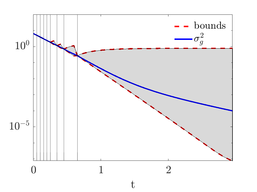
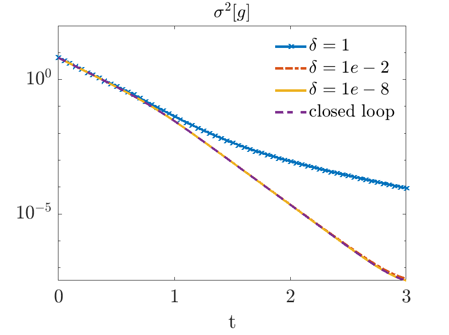
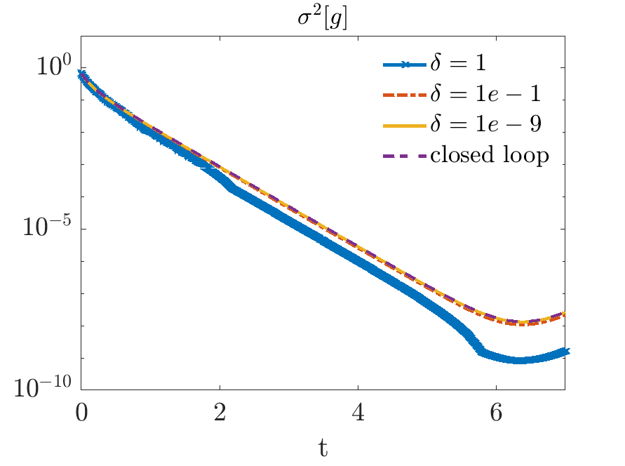
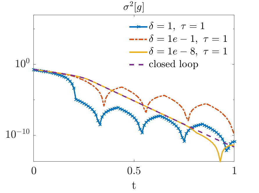
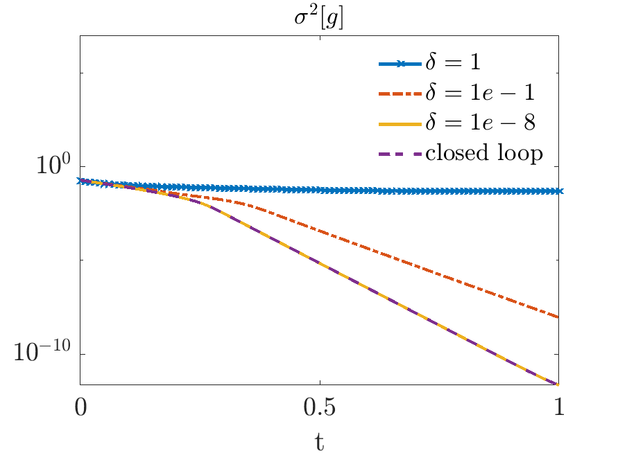
To better interpret these results, we perform a numerical analysis to study the decay of the variance σ2[g]superscript𝜎2delimited-[]𝑔\sigma^{2}[g] using different values of δ𝛿\delta in Algorithm 1 and Algorithm 2. Figure 5.5 compares the variance of the system as the values of the tolerance δ𝛿\delta changes. It can be seen that as δ𝛿\delta decreases, the MdPC(σ2superscript𝜎2\sigma^{2}) approaches the closed-loop control. This numerical evidence is further confirmed by Table 5.2. With decreasing values of δ𝛿\delta we have an increasing number of updates and the values of the functional JΔt,Nssubscript𝐽Δ𝑡subscript𝑁𝑠J_{\Delta t,N_{s}} computed in (5.5) is similar for the three control approaches. We observe that the closed-loop control corresponds to a limit case of the moment-driven MPC methods.
Refer to caption
Refer to caption
Figure 5.5: Test 1. Semi-log plot with a comparison between variance decay with different values of the tolerance δ𝛿\delta. Left: variance decays for MdPC(m1,σ2)subscript𝑚1superscript𝜎2(m_{1},\sigma^{2}). Right: decays for MdPC(σ2superscript𝜎2\sigma^{2}) compared with respect to the closed-loop control.
MdPC(m1,σ2subscript𝑚1superscript𝜎2m_{1},\sigma^{2}) MdPC(σ2superscript𝜎2\sigma^{2})
δ𝛿\delta 1 0.10.10.1 1e-8 1 0.1 1e-8
update (%percent\%) 4 % 8% 71 % 0 % 4 % 72 %
σ2[g](T)superscript𝜎2delimited-[]𝑔𝑇\sigma^{2}[g](T) 1.28e-11 1.26e-10 3.80e-12 5.04e-2 8.94e-9 2.22e-12
JΔt,Nssubscript𝐽Δ𝑡subscript𝑁𝑠J_{\Delta t,N_{s}} 1.8131 0.1306 0.1281 0.1777 0.1309 0.1281

Table 5.2: Test 1. We compare the different MdPC approaches with respect to the closed-loop control. For MdPC(m1,σ2subscript𝑚1superscript𝜎2m_{1},\sigma^{2}) the tolerance for the mean is set τ=1𝜏1\tau=1. The number of updates indicates the percentage of control updates over the total number of time steps NT=100subscript𝑁𝑇100N_{T}=100 (for reference, the closed-loop control would require a 100%). The final value of the variance is denoted by σ2(T)superscript𝜎2𝑇\sigma^{2}(T), and JΔt,Nssubscript𝐽Δ𝑡subscript𝑁𝑠J_{\Delta t,N_{s}} corresponds to the value of the cost functional (5.5). For the closed-loop control σ2(T)=3.80e12superscript𝜎2𝑇3.80𝑒12\sigma^{2}(T)=3.80e-12 and JΔt,Ns=0.1281subscript𝐽Δ𝑡subscript𝑁𝑠0.1281J_{\Delta t,N_{s}}=0.1281.

5.2 Test 2: Cucker-Smale dynamics

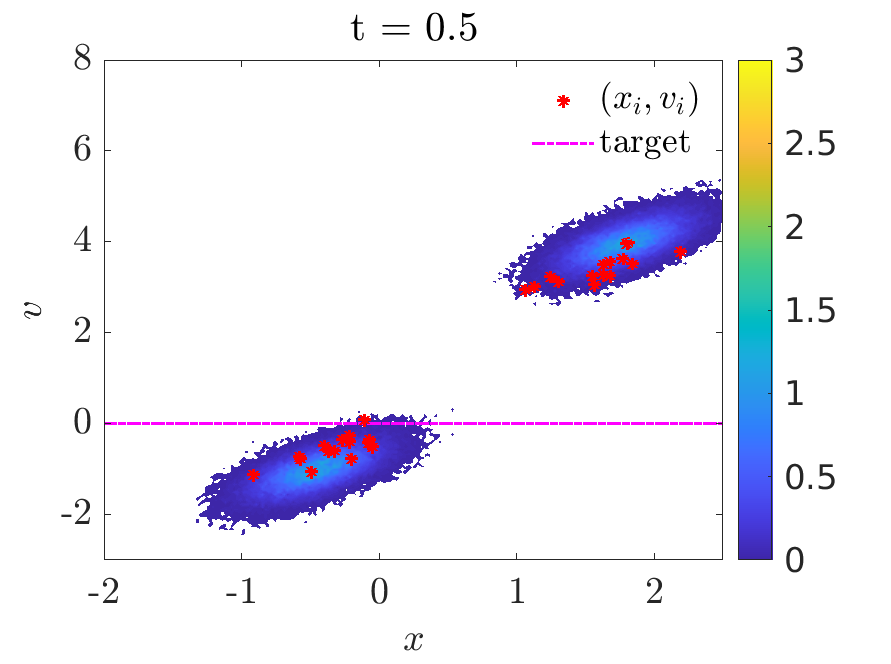
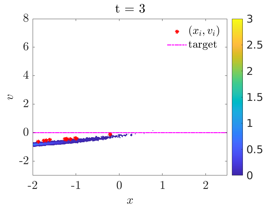
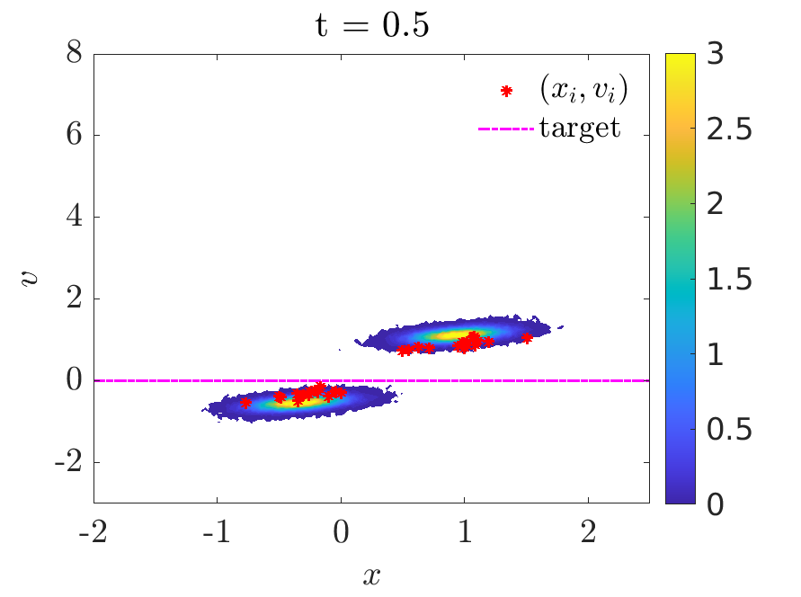
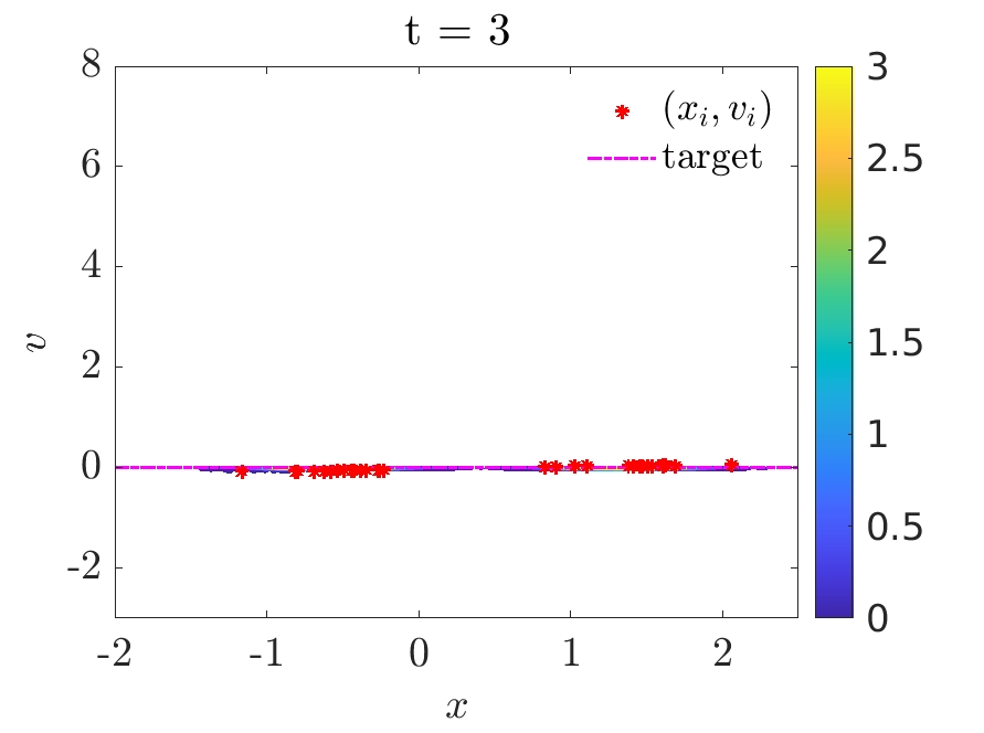
We study alignment in a second-order, 1D model with Cucker-Smale type interactions [27]. We consider a state characterized by (xi,vi)2subscript𝑥𝑖subscript𝑣𝑖superscript2(x_{i},v_{i})\in\mathbb{R}^{2}. The interaction kernel is given by P(x,y)=1(1+|yx|2)γ,𝑃𝑥𝑦1superscript1superscript𝑦𝑥2𝛾P(x,y)=\frac{1}{(1+|y-x|^{2})^{\gamma}}, with γ0,𝛾0\gamma\geq 0, which is a decreasing function of the relative distance, bounded to [0,1]01[0,1]. Under the condition γ1/2𝛾12\gamma\geq 1/2, the convergence to consensus of the free dynamics depends on the initial state [27]. We set γ=2𝛾2\gamma=2 and a suitable initial state, such that the flocking state is not achieved without control action. To perform our analysis we refer to the second-order dynamics (2.20) and use Remark 2.1 to obtain the Riccati equations. Unlike the first-order dynamics, the constrained mean-field has a transport term

(5.6) tg+vxg=v(g(𝒫[g]+u(t))),g(x,v,0)=g0(x,v),formulae-sequencesubscript𝑡𝑔𝑣subscript𝑥𝑔subscript𝑣𝑔𝒫delimited-[]𝑔𝑢𝑡𝑔𝑥𝑣0superscript𝑔0𝑥𝑣\partial_{t}g+v\cdot\nabla_{x}g=-\nabla_{v}\cdot\left(g\left(\mathcal{P}[g]+u(t)\right)\right),\qquad\qquad\,\,g(x,v,0)=g^{0}(x,v),

and the nonlocal operator 𝒫𝒫\mathcal{P} is defined as

𝒫[g](x,v,t)=d×dP(x,y)(wv)g(y,w,t)𝑑y𝑑w.𝒫delimited-[]𝑔𝑥𝑣𝑡subscriptsuperscript𝑑superscript𝑑𝑃𝑥𝑦𝑤𝑣𝑔𝑦𝑤𝑡differential-d𝑦differential-d𝑤\mathcal{P}[g](x,v,t)=\int_{\mathbb{R}^{d}\times\mathbb{R}^{d}}P(x,y)(w-v)g(y,w,t)\ dy\ dw.

We discretize the mean-field model employing the forward scheme (5.1) with fixed time step Δt=0.05Δ𝑡0.05\Delta t=0.05, sampling size of Ns=100000subscript𝑁𝑠100000N_{s}=100000 particles and fixed M=100𝑀100M=100. In order to treat the additional transport term in the dynamics, we use a splitting method to perform the free transport step. The control is computed by means of MdPC(σ2superscript𝜎2\sigma^{2}). We refer to Table (5.1) for the choice of parameters.

Figure 5.6 presents the initial data at the top, which is a bivariate distribution unimodal in space and bimodal in velocity defined as follows:

g0(x,v)=14πσxσvexp(x22σx2)[exp((v+v)22σv2)+exp((v+v+)22σv2)],superscript𝑔0𝑥𝑣14𝜋subscript𝜎𝑥subscript𝜎𝑣expsuperscript𝑥22superscriptsubscript𝜎𝑥2delimited-[]expsuperscript𝑣subscript𝑣22superscriptsubscript𝜎𝑣2expsuperscript𝑣subscript𝑣22superscriptsubscript𝜎𝑣2g^{0}(x,v)=\frac{1}{4\pi\sigma_{x}\sigma_{v}}\text{exp}\Biggl{(}-\frac{x^{2}}{2\sigma_{x}^{2}}\Biggr{)}\Biggl{[}\text{exp}\Biggl{(}-\frac{(v+v_{-})^{2}}{2\sigma_{v}^{2}}\Biggr{)}+\text{exp}\Biggl{(}-\frac{(v+v_{+})^{2}}{2\sigma_{v}^{2}}\Biggr{)}\Biggr{]},

with σx=0.2,σv=0.4formulae-sequencesubscript𝜎𝑥0.2subscript𝜎𝑣0.4\sigma_{x}=0.2,\sigma_{v}=0.4 and v=1,v+=4formulae-sequencesubscript𝑣1subscript𝑣4v_{-}=-1,v_{+}=4. We compare the evolution of the density distribution in the phase space (x,v)𝑥𝑣(x,v), jointly with a set of N=30𝑁30N=30 microscopic points (xi(t),vi(t))subscript𝑥𝑖𝑡subscript𝑣𝑖𝑡(x_{i}(t),v_{i}(t)) sampled from the initial distribution. The middle row depicts two time frames of the uncontrolled dynamics, where alignment is not reached. In the bottom row we report the constrained dynamics, where the alignment is reached at time T=3𝑇3T=3 and the density g(x,v,t)𝑔𝑥𝑣𝑡g(x,v,t) concentrates at the target state v¯=0¯𝑣0\bar{v}=0, whereas its support is bounded in space.
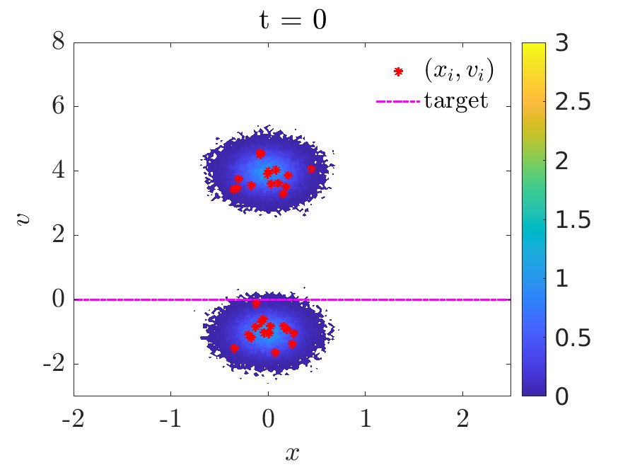
Refer to caption

Uncontrolled

Refer to caption
Refer to caption

MdPC(σ2)MdPCsuperscript𝜎2\textrm{MdPC}(\sigma^{2})

Refer to caption
Refer to caption
Figure 5.6: Test 2. Comparison between the uncontrolled and controlled mean-field evolution of the Cucker-Smale dynamics with MdPC(σ2)MdPCsuperscript𝜎2\textrm{MdPC}(\sigma^{2}) and δ=1𝛿1\delta=1. Without control intervention the alignment state is not reached.
Refer to caption
Refer to caption
Figure 5.7: Test 2.Left: variance and bounds for the second order attractive one-dimensional mean-field dynamics with tolerance δ=1𝛿1\delta=1. Right: variance decays with different values of δ𝛿\delta.

We perform a numerical study for the variance decay σ2[g]superscript𝜎2delimited-[]𝑔\sigma^{2}[g] using different tolerances δ𝛿\delta in Algorithm 1 for MdPC(σ2)MdPCsuperscript𝜎2\textrm{MdPC}(\sigma^{2}). Figure 5.7 compares the decay of the variance of the system as the values of the tolerance δ𝛿\delta changes. On the left we observe the decay for δ=1𝛿1\delta=1 jointly with the update and the evolution of the variance bounds. On the right, it can be seen that as δ𝛿\delta decreases MdPC(σ2)MdPCsuperscript𝜎2\textrm{MdPC}(\sigma^{2}) is similar to the closed-loop control dynamics. Table 5.3 quantifies the performances of the MdPC(σ2superscript𝜎2\sigma^{2}) reporting the percentage of control updates performed over NT=60subscript𝑁𝑇60N_{T}=60 steps, the variance σ2[g]superscript𝜎2delimited-[]𝑔\sigma^{2}[g] at time T=3𝑇3T=3, and the value of the cost functional (5.5).

MdPC(σ2superscript𝜎2\sigma^{2}) closed-loop
δ𝛿\delta 1 1e-2 1e-8 - -
update (%percent\%) 13 % 40 % 99 % 100%
σ2[g](T)superscript𝜎2delimited-[]𝑔𝑇\sigma^{2}[g](T) 9.1393e-05 3.9247e-08 3.3374e-08 3.3371e-08
JΔt,Nssubscript𝐽Δ𝑡subscript𝑁𝑠J_{\Delta t,N_{s}} 3.0059 2.9976 2.9951 2.9951
Table 5.3: Test 2. Number of updates and final values of the variance using different values of δ𝛿\delta. We compare the different control approaches. The update percentage is computed over NT=60subscript𝑁𝑇60N_{T}=60.

5.3 Test 3: Aggregation dynamics

The last example is a first-order aggregation model in 2D, where agents interact according to an attraction-repulsion kernel. We consider the following interaction kernel P(v,w)=|wv|α2|wv|β2,𝑃𝑣𝑤superscript𝑤𝑣𝛼2superscript𝑤𝑣𝛽2P(v,w)=|w-v|^{\alpha-2}-|w-v|^{\beta-2}, where α=4𝛼4\alpha=4 and β=2𝛽2\beta=2. For these specific values of the parameters it can be shown that the equilibrium configuration is an uniform distribution on an annulus of radius R=13𝑅13R=\frac{1}{\sqrt{3}}, and same center of mass as the initial distribution. For analytical and numerical characterizations of the equilbrium of these models we refer to [13]. We consider an initial density of particles uniformly distributed on the 2D disc of radius R0=23subscript𝑅023R_{0}=\frac{2}{\sqrt{3}} centered in (1,1)11(-1,1), that is

(5.7) g0(v)=1|𝒞|χ𝒞(v),𝒞:={v2:|v(1,1)|R0},formulae-sequencesuperscript𝑔0𝑣1𝒞subscript𝜒𝒞𝑣assign𝒞conditional-set𝑣superscript2𝑣superscript11topsubscript𝑅0g^{0}(v)=\frac{1}{|\mathcal{C}|}\chi_{\mathcal{C}}(v)\,,\qquad\mathcal{C}:=\{v\in\mathbb{R}^{2}:|v-(-1,1)^{\top}|\leq R_{0}\}\,,

and |𝒞|𝒞|\mathcal{C}| denoting its volume. In order to simulate the dynamics we consider Ns=105subscript𝑁𝑠superscript105N_{s}=10^{5} particles sampled from g0(v)superscript𝑔0𝑣g^{0}(v) and we implement the forward scheme (5.1) with fixed time step Δt=0.01Δ𝑡0.01\Delta t=0.01. We select M=10𝑀10M=10 particles for the approximation of the non-local interactions. We use the MdPC(σ2superscript𝜎2\sigma^{2}) approach with a penalization factor ν=1𝜈1\nu=1 and a stopping tolerance δ=0.1𝛿0.1\delta=0.1. In Figure 5.8 we report the evolution of the mean-field and the microscopic dynamics. The latter is sampled with N=30𝑁30N=30 particles from g0superscript𝑔0g^{0}. The second row of Figure 5.4 shows the uncontrolled dynamics, where mass concentrates towards a 2D annulus of radius R=13𝑅13R=\frac{1}{\sqrt{3}}. While the third row depicts the open-loop control case where MdPC(σ2superscript𝜎2\sigma^{2}) is applied. At time T=7𝑇7T=7 the distribution is converged to a concentration at v¯=(v¯1,v¯2)=(0,0)¯𝑣subscript¯𝑣1subscript¯𝑣200\bar{v}=(\bar{v}_{1},\bar{v}_{2})=(0,0).

As in previous tests we illustrates a comparison between different open-loop controls varying tolerance δ𝛿\delta in algorithms 1. Figure 5.9 and Table 5.4 highlight that with a very small value of δ𝛿\delta, the MdPC approach coincides with the closed-loop approach.
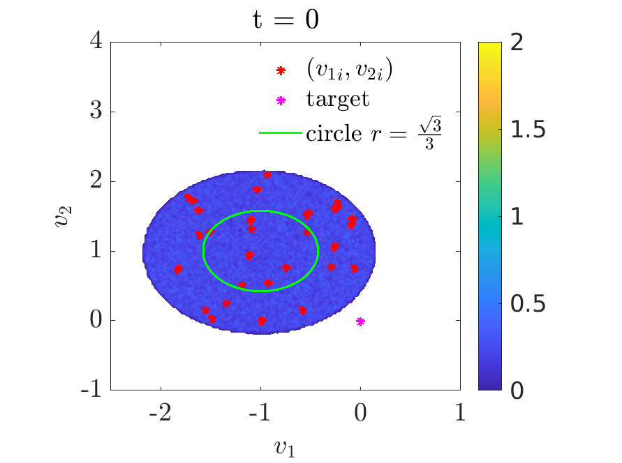
Refer to caption

Uncontrolled dynamics

Refer to caption
Refer to caption

MdPC(σ2)MdPCsuperscript𝜎2\textrm{MdPC}(\sigma^{2})

Refer to caption
Refer to caption
Figure 5.8: Test 3. Comparison between the uncontrolled and controlled mean-field evolution of the aggregation dynamics with MdPC(σ2)MdPCsuperscript𝜎2\textrm{MdPC}(\sigma^{2}) and δ=0.1𝛿0.1\delta=0.1. Without control intervention the alignment state is not reached.
Refer to caption
Refer to caption
Figure 5.9: Test 3. Left: variance evolution and bounds for the first order attractive-repulsive one-dimensional mean-field dynamics with tolerance δ=0.1𝛿0.1\delta=0.1. Right: variance decays with different values of δ𝛿\delta.
MdPC(σ2superscript𝜎2\sigma^{2}) closed-loop
δ𝛿\delta 1 1e-1 1e-9 - -
update (%percent\%) 1 % 4 % 99 % 100%
σ2[g](T)superscript𝜎2delimited-[]𝑔𝑇\sigma^{2}[g](T) 1.6875e-09 2.1253e-08 2.6151e-08 2.6187e-08
JΔt,Nssubscript𝐽Δ𝑡subscript𝑁𝑠J_{\Delta t,N_{s}} 3.0459 2.9751 2.9750 2.9750
Table 5.4: Test 3: Aggregation dynamics. Number of updates and final values of the variance using different values of δ𝛿\delta. The update percentage is computed over NT=700subscript𝑁𝑇700N_{T}=700.
Concluding Remarks

We have studied the design of control laws for interacting particle system based on the solution of the optimal control problem associated to linearized dynamics. We have assessed the impact of different sub-optimal control laws into the original non-linear dynamics deriving mean-field limits of the microscopic constrained systems and estimating analytically and numerically the decay of the first and second moments. We proposed a novel numerical technique based on the moments decay (MdPC). In particular, we obtain a hierarchy of approximations from open-loop to closed-loop control by scaling the tolerance level. These strategies have shown to be robust even with considerably fewer updates of the control law for the non-linear dynamics. The proposed methodology expands the existing NMPC literature by developing a new paradigm in which the control laws are updated based on dynamic information of the system. Here, the use of moments information is a particular example suitable in the context of mean-field dynamics. Further extensions and analysis will include the study of other dynamic indicators for control update, in particular those that could be linked to a physical observable of the system, and the incorporation of nonlinear state estimation in the control loop.

References

  • [1] M. Aduamoah, B. D. Goddard, J. W. Pearson, and J. C. Roden. PDE-Constrained optimization models and pseudospectral methods for multiscale particle dynamics. arXiv:2009.09850, 2020.
  • [2] G. Albi, N. Bellomo, L. Fermo, S.-Y. Ha, J. Kim, L. Pareschi, D. Poyato, and J. Soler. Vehicular traffic, crowds, and swarms: from kinetic theory and multiscale methods to applications and research perspectives. Math. Models Methods Appl. Sci., 29(10):1901–2005, 2019.
  • [3] G. Albi, M. Bongini, E. Cristiani, and D. Kalise. Invisible control of self-organizing agents leaving unknown environments. SIAM J. Appl. Math., 76(4):1683–1710, 2016.
  • [4] G. Albi, Y.-P. Choi, M. Fornasier, and D. Kalise. Mean field control hierarchy. Appl. Math. Optim., 76(1):93–135, 2017.
  • [5] G. Albi, M. Herty, and L. Pareschi. Kinetic description of optimal control problems and applications to opinion consensus. Commun. Math. Sci., 13(6):1407–1429, 2015.
  • [6] G. Albi and D. Kalise. (sub)optimal feedback control of mean field multi-population dynamics. IFAC-PapersOnLine, 51(3):86 – 91, 2018.
  • [7] G. Albi and L. Pareschi. Binary interaction algorithms for the simulation of flocking and swarming dynamics. Multiscale Model. Simul., 11(1):1–29, 2013.
  • [8] G. Albi, L. Pareschi, and M. Zanella. Boltzmann-type control of opinion consensus through leaders. Philos. Trans. R. Soc. Lond. Ser. A Math. Phys. Eng. Sci., 372(2028):20140138, 18, 2014.
  • [9] B. Azmi, D. Kalise, and K. Kunisch. Optimal feedback law recovery by gradient-augmented sparse polynomial regression. arXiv:2007.09753, 2020.
  • [10] B. Azmi and K. Kunisch. A hybrid finite-dimensional RHC for stabilization of time-varying parabolic equations. SIAM J. Control Optim., 57(5):3496–3526, 2019.
  • [11] H. Babovsky and H. Neunzert. On a simulation scheme for the boltzmann equation. Math. Methods Appl. Sci., 8(1):223–233, 1986.
  • [12] R. Bailo, M. Bongini, J. A. Carrillo, and D. Kalise. Optimal consensus control of the cucker-smale model. IFAC-PapersOnLine, 51(13):1 – 6, 2018.
  • [13] D. Balagué, J. A. Carrillo, T. Laurent, and G. Raoul. Nonlocal interactions by repulsive-attractive potentials: radial ins/stability. Phys. D, 260:5–25, 2013.
  • [14] N. Bellomo and J. Soler. On the mathematical theory of the dynamics of swarms viewed as complex systems. Math. Models Methods Appl. Sci., 22(suppl. 1):1140006, 29, 2012.
  • [15] A. Bobylev and K. Nanbu. Theory of collision algorithms for gases and plasmas based on the Boltzmann equation and the Landau-Fokker-Planck equation. Phys. Rev. E, 61(4):4576, 2000.
  • [16] L. Boudin and F. Salvarani. A kinetic approach to the study of opinion formation. M2AN Math. Model. Numer. Anal., 43(3):507–522, 2009.
  • [17] A. Bressan and B. Piccoli. Introduction to the mathematical theory of control, volume 1. American institute of mathematical sciences Springfield, 2007.
  • [18] L. M. Briceño Arias, D. Kalise, and F. J. Silva. Proximal methods for stationary mean field games with local couplings. SIAM J. Control Optim., 56(2):801–836, 2018.
  • [19] M. Burger, R. Pinnau, C. Totzeck, O. Tse, and A. Roth. Instantaneous control of interacting particle systems in the mean-field limit. J. Comput. Phys., 405:109181, 20, 2020.
  • [20] E. F. Camacho and C. B. Alba. Model predictive control. Springer Science & Business Media, 2013.
  • [21] J. A. Canizo, J. A. Carrillo, and J. Rosado. A well-posedness theory in measures for some kinetic models of collective motion. Math. Models Methods Appl. Sci., 21(03):515–539, 2011.
  • [22] M. Caponigro, M. Fornasier, B. Piccoli, and E. Trélat. Sparse stabilization and control of alignment models. Math. Models Methods Appl. Sci., 25(3):521–564, 2015.
  • [23] J. A. Carrillo, Y.-P. Choi, and M. Hauray. The derivation of swarming models: mean-field limit and Wasserstein distances. In Collective dynamics from bacteria to crowds, pages 1–46. Springer, 2014.
  • [24] Y.-P. Choi, D. Kalise, J. Peszek, and A. A. Peters. A collisionless singular Cucker-Smale model with decentralized formation control. SIAM J. Appl. Dyn. Syst., 18(4):1954–1981, 2019.
  • [25] S. Cordier, L. Pareschi, and G. Toscani. On a kinetic model for a simple market economy. J. Stat. Phys., 120(1-2):253–277, 2005.
  • [26] E. Cristiani, B. Piccoli, and A. Tosin. Multiscale modeling of pedestrian dynamics, volume 12 of MS&A. Model. Simul. Appl. Springer, Cham, 2014.
  • [27] F. Cucker and S. Smale. Emergent behavior in flocks. IEEE Trans. Automat. Control, 52(5):852–862, 2007.
  • [28] P. Degond, S. Göttlich, M. Herty, and A. Klar. A network model for supply chains with multiple policies. Multiscale Model. Simul., 6(3):820–837, 2007.
  • [29] P. Degond, M. Herty, and J.-G. Liu. Flow on sweeping networks. Multiscale Model. Simul., 12(2):538–565, 2014.
  • [30] P. Degond, J.-G. Liu, S. Motsch, and V. Panferov. Hydrodynamic models of self-organized dynamics: derivation and existence theory. Methods Appl. Anal., 20(2):89–114, 2013.
  • [31] P. Degond and S. Motsch. Continuum limit of self-driven particles with orientation interaction. Math. Models Methods Appl. Sci., 18(suppl.):1193–1215, 2008.
  • [32] G. Dimarco, R. Caflisch, and L. Pareschi. Direct simulation Monte Carlo schemes for coulomb interactions in plasmas. Commun. Appl. Ind. Math., 1(1):72–91, 2010.
  • [33] S. Dolgov, D. Kalise, and K. Kunisch. Tensor decompositions for high-dimensional hamilton-jacobi-bellman equations. arXiv:1908.01533, 2019.
  • [34] J. R. Dyer, A. Johansson, D. Helbing, I. D. Couzin, and J. Krause. Leadership, consensus decision making and collective behaviour in humans. Philos. Trans. Roy. Soc. B, 364(1518):781–789, 2009.
  • [35] M. R. D’Orsogna, Y.-L. Chuang, A. L. Bertozzi, and L. S. Chayes. Self-propelled particles with soft-core interactions: patterns, stability, and collapse. Phys. Rev. Lett., 96(10):104302, 2006.
  • [36] A. Eqtami, D. V. Dimarogonas, and K. J. Kyriakopoulos. Event-based model predictive control for the cooperation of distributed agents. In 2012 Amer. Control Conf., pages 6473–6478.
  • [37] G. Estrada-Rodriguez and H. Gimperlein. Interacting particles with Lévy strategies: limits of transport equations for swarm robotic systems. SIAM J. Appl. Math., 80(1):476–498, 2020.
  • [38] M. Fornasier, J. Haskovec, and G. Toscani. Fluid dynamic description of flocking via the Povzner-Boltzmann equation. Phys. D, 240(1):21–31, 2011.
  • [39] M. Fornasier, S. Lisini, C. Orrieri, and G. Savaré. Mean-field optimal control as gamma-limit of finite agent controls. European J. Appl. Math., 30(6):1153–1186, 2019.
  • [40] M. Fornasier, B. Piccoli, and F. Rossi. Mean-field sparse optimal control. Philos. Trans. R. Soc. Lond. Ser. A Math. Phys. Eng. Sci., 372(2028):20130400, 21, 2014.
  • [41] M. Fornasier and F. Solombrino. Mean-field optimal control. ESAIM Control Optim. Calc. Var., 20(4):1123–1152, 2014.
  • [42] G. Freudenthaler and T. Meurer. PDE-based multi-agent formation control using flatness and backstepping: analysis, design and robot experiments. Automatica, 115:108897, 13, 2020.
  • [43] J. Garnier, G. Papanicolaou, and T.-W. Yang. Consensus convergence with stochastic effects. Vietnam J. Math., 45(1-2):51–75, 2017.
  • [44] J. Gómez-Serrano, C. Graham, and J.-Y. Le Boudec. The bounded confidence model of opinion dynamics. Math. Models Methods Appl. Sci., 22(2):1150007, 46, 2012.
  • [45] L. Grüne and J. Pannek. Nonlinear model predictive control. In Nonlinear model predictive control, pages 45–69. Springer, 2017.
  • [46] S.-Y. Ha and E. Tadmor. From particle to kinetic and hydrodynamic descriptions of flocking. Kinet. Relat. Models, 1(3):415–435, 2008.
  • [47] Y. Han, A. Hegyi, Y. Yuan, S. Hoogendoorn, M. Papageorgiou, and C. Roncoli. Resolving freeway jam waves by discrete first-order model-based predictive control of variable speed limits. Transportation Research Part C: Emerging Technologies, 77:405–420, 2017.
  • [48] R. Hegselmann, U. Krause, et al. Opinion dynamics and bounded confidence models, analysis, and simulation. Journal of artificial societies and social simul., 5(3), 2002.
  • [49] M. Herty and D. Kalise. Suboptimal nonlinear feedback control laws for collective dynamics. In 2018 IEEE 14th Intern. Conf. on Control and Automat. (ICCA), pages 556–561.
  • [50] M. Herty and L. Pareschi. Fokker-Planck asymptotics for traffic flow models. Kinet. Relat. Models, 3(1):165–179, 2010.
  • [51] M. Herty, L. Pareschi, and S. Steffensen. Mean–field control and Riccati equations. Netw. Heterog. Media, 10(3):699, 2015.
  • [52] M. Herty and C. Ringhofer. Averaged kinetic models for flows on unstructured networks. Kinet. Relat. Models, 4(4):1081–1096, 2011.
  • [53] M. Herty and C. Ringhofer. Feedback controls for continuous priority models in supply chain management. Comput. Methods Appl. Math., 11(2):206–213, 2011.
  • [54] M. Herty and M. Zanella. Performance bounds for the mean-field limit of constrained dynamics. Discrete Contin. Dyn. Syst., 37(4):2023, 2017.
  • [55] S. Jin, L. Li, and J.-G. Liu. Random Batch Methods (RBM) for interacting particle systems. J. Comput. Phys., 400:108877, 2020.
  • [56] S. Liu, M. Jacobs, W. Li, L. Nurbekyan, and S. J. Osher. Computational methods for nonlocal mean field games with applications.
  • [57] D. Q. Mayne, J. B. Rawlings, C. V. Rao, and P. O. Scokaert. Constrained model predictive control: Stability and optimality. Automatica, 36(6):789–814, 2000.
  • [58] S. Motsch and E. Tadmor. Heterophilious dynamics enhances consensus. SIAM review, 56(4):577–621, 2014.
  • [59] K.-K. Oh, M.-C. Park, and H.-S. Ahn. A survey of multi-agent formation control. Automatica, 53:424–440, 2015.
  • [60] A. A. Peters, R. H. Middleton, and O. Mason. Leader tracking in homogeneous vehicle platoons with broadcast delays. Automatica, 50(1):64–74, 2014.
  • [61] M. Petrovitch. Sur une manière d’étendre le théorème de la moyenne aux équations différentielles du premier ordre. Mathematische Annalen, 54:417–436, 1901.
  • [62] R. E. Stern, S. Cui, M. L. Delle Monache, R. Bhadani, M. Bunting, M. Churchill, N. Hamilton, H. Pohlmann, F. Wu, B. Piccoli, et al. Dissipation of stop-and-go waves via control of autonomous vehicles: Field experiments. Transp. Research Part C: Emerging Techn., 89:205–221, 2018.
  • [63] G. Toscani. Kinetic models of opinion formation. Commun. Math. Sci., 4(3):481–496, 2006.
  • [64] A. Tosin and M. Zanella. Kinetic-controlled hydrodynamics for traffic models with driver-assist vehicles. Multiscale Model. Simul., 17(2):716–749, 2019.
  • [65] P. Varutti, B. Kern, T. Faulwasser, and R. Findeisen. Event-based model predictive control for networked control systems. In Proc. of the 48h IEEE Conf. on Decision and Control (CDC) held jointly with 2009 28th Chinese Control Conf., pages 567–572, 2009.