Flow Curvature Manifold and Energy
of Generalized Liénard Systems

Abstract.

In his famous book entitled Theory of Oscillations, Nicolas Minorsky wrote: “each time the system absorbs energy the curvature of its trajectory decreases and vice versa”. According to the Flow Curvature Method, the location of the points where the curvature of trajectory curve, integral of such planar singularly dynamical systems, vanishes directly provides a first order approximation in $\varepsilon$ of its slow invariant manifold equation. By using this method, we prove that, in the $\varepsilon$-vicinity of the slow invariant manifold of generalized Liénard systems, the curvature of trajectory curve increases while the energy of such systems decreases. Hence, we prove Minorsky’s statement for the generalized Liénard systems. Then, we establish a relationship between curvature and energy for such systems. These results are then exemplified with the classical Van der Pol and generalized Liénard singularly perturbed systems.

1. Introduction

At the end of the 1930s, a general equation of self-sustained oscillations (1) was stated by the French engineer Alfred Liénard [34]. It encompassed the prototypical equation of the Dutch physicist Balthasar Van der Pol [45] modelling the so-called relaxation oscillations.

(1) $$\dfrac{d^{2}x}{dt^{2}}+\omega f\left(x\right)\dfrac{dx}{dt}+\omega^{2}x=0.$$

Less than fifteen years later, a more general form was provided by the American mathematicians Norman Levinson and his former student Oliver K. Smith [32]:

(2) $$\dfrac{d^{2}x}{dt^{2}}+\mu f\left(x\right)\dfrac{dx}{dt}+g\left(x\right)=0.$$

At that time, the classical geometric theory of differential equations developed originally by Andronov [1], Tikhonov [44] and Levinson [33] stated that singularly perturbed systems possess invariant manifolds on which trajectories evolve slowly, and toward which nearby orbits contract exponentially in time (either forward or backward) in the normal directions. These manifolds have been called asymptotically stable (or unstable) slow invariant manifolds. Then, Fenichel [5, 6, 7, 8] theory for the persistence of normally hyperbolic invariant manifolds enabled to establish the local invariance of slow invariant manifolds that possess both expanding and contracting directions and which were labeled slow invariant manifolds.

During the last century, various methods have been developed to compute the slow invariant manifold or, at least an asymptotic expansion in power of $\varepsilon$. The seminal works of Wasow [46], Cole [3], O’Malley [37, 38] and Fenichel [5, 6, 7, 8] to name but a few, gave rise to the so-called Geometric Singular Perturbation Method. According to this theory, existence as well as local invariance of the slow invariant manifold of singularly perturbed systems has been stated. Then, the determination of the slow invariant manifold equation turned into a regular perturbation problem in which one generally expected the asymptotic validity of such expansion to breakdown [38]. Fifteen years ago, a new approach of $n$-dimensional singularly perturbed dynamical systems of ordinary differential equations with two time scales, called Flow Curvature Method has been developed [19]. In dimension two, it consists in considering the trajectory curves integral of such systems as plane curves. Based on the use of local metric properties of curvature resulting from Differential Geometry, this method which does not require the use of asymptotic expansions, states that the location of the points where the local curvature of trajectory curves of such systems, vanishes, directly provides a first order approximation in $\varepsilon$ of the slow invariant manifold equation associated with such two-dimensional or planar singularly perturbed systems. This method gives an implicit non intrinsic equation, because it depends on the euclidean metric. A ’kinetic energy metric’ has been introduced in [28] for chemical kinetic systems and an extremum principle for computing slow invariant manifolds has been formulated [29, 30] which can be viewed as minimum curvature geodesics. In [21] a curvature-based differential geometry formulation for the slow manifold problem has been used for the purpose of a coordinate-independent formulation of the invariance equation.

In his famous book entitled Theory of Oscillations, the Russian mathematician Nicolas Minorsky [39] wrote:

“each time the system absorbs energy the curvature of its trajectory decreases and vice versa when the energy is supplied by the system (e. g. braking) the curvature increases.”

Thus, according to Minorsky, energy and curvature of the trajectory are linked by a relationship that he unfortunately didn’t give. So, the aim of this work is to prove this statement in the $\varepsilon$-vicinity of the slow invariant manifold of generalized Liénard systems and to establish this relationship for such systems. The paper is organized as follows. In section 2, we briefly present the definitions of singularly perturbed systems. Then, we prove that generalized Liénard systems are planar singularly perturbed systems. In section 3, we recall Liénard’s assumptions for which the generalized Liénard systems has a unique stable limit cycle and so, a slow invariant manifold. In section 4, we recall the main features of the Flow Curvature Method according to which the curvature of the trajectory curve, integral of planar singularly perturbed systems defines a flow curvature manifold and we state that the location of the points where this manifold vanishes directly provides a first order approximation in $\varepsilon$ of its slow invariant manifold equation. Then, we prove Minorsky’s statement for the generalized Liénard systems and establish a relationship between curvature and energy for such systems. In section 5, we exemplify these results with the classical Van der Pol singularly perturbed system. Discussion and perspectives are presented in section 6.

2. Singularly perturbed systems

Thus, according to Tikhonov [44], Takens [43], Jones [23] and Kaper [24] singularly perturbed systems may be defined such as:

(3) $$\begin{array}[]{*{20}c}{{\vec{x}}^{\prime}=\vec{f}\left({\vec{x},\vec{y},\varepsilon}\right),\mbox{ }\hfill}\\ {{\vec{y}}^{\prime}=\varepsilon\vec{g}\left({\vec{x},\vec{y},\varepsilon}\right)}.\hfill\\ \end{array}$$

where $\vec{x}\in\mathbb{R}^{m}$, $\vec{y}\in\mathbb{R}^{p}$, $\varepsilon\in\mathbb{R}^{+}$, and the prime denotes differentiation with respect to the independent variable $t$. The functions $\vec{f}$ and $\vec{g}$ are assumed to be $C^{\infty}$ functions of $\vec{x}$, $\vec{y}$ and $\varepsilon$ in $U\times I$, where $U$ is an open subset of $\mathbb{R}^{m}\times\mathbb{R}^{p}$ and $I$ is an open interval containing $\varepsilon=0$.

In the case when $0<\varepsilon\ll 1$, i.e., $\varepsilon$ is a small positive number, the variable $\vec{x}$ is called fast variable, and $\vec{y}$ is called slow variable. Using Landau’s notation: $O\left({\varepsilon^{k}}\right)$ represents a function $f$ of $x$ and $\varepsilon$ such that $f(u,\varepsilon)/\varepsilon^{k}$ is bounded for positive $\varepsilon$ going to zero, uniformly for $u$ in the given domain. It is used to consider that generally $\vec{x}$ evolves at an $O\left(1\right)$ rate; while $\vec{y}$ evolves at an $O\left(\varepsilon\right)$ slow rate. Reformulating system (3) in terms of the rescaled variable $\tau=\varepsilon t$, we obtain

(4) $$\varepsilon\dot{\vec{x}} =\vec{f}\left({\vec{x},\vec{y},\varepsilon}\right),$$

$$\dot{\vec{y}} =\vec{g}\left({\vec{x},\vec{y},\varepsilon}\right).$$

The dot represents the derivative with respect to the new independent variable $\tau$.

The independent variables $t$ and $\tau$ are referred to the fast and slow times, respectively, and (3) and (4) are called the fast and slow systems, respectively. These systems are equivalent whenever $\varepsilon\neq 0$, and they are labeled singular perturbation problems when $0<\varepsilon\ll 1$. The label “singular” stems in part from the discontinuous limiting behavior in system (3) as $\varepsilon\to 0$.

In such case system (4) leads to a differential-algebraic system called reduced slow system whose dimension decreases from $m+p=n$ to $p$. Then, the slow variable $\vec{y}\in\mathbb{R}^{p}$ partially evolves in the submanifold $M_{0}$ called the critical manifold and defined by

(5) $$M_{0}:=\left\{{\left({\vec{x},\vec{y}}\right):\vec{f}\left({\vec{x},\vec{y},0}\right)={\vec{0}}}\right\}.$$

When $D_{x}f$ is invertible, thanks to Implicit Function Theorem, $M_{0}$ is given by the graph of a $C^{\infty}$ function $\vec{y}=\vec{F}_{0}\left(\vec{x}\right)$ for $\vec{x}\in D$, where $D\subseteq\mathbb{R}^{p}$ is a compact, simply connected domain and the boundary of $D$ is an $(p-1)$–dimensional $C^{\infty}$ submanifold.

According to Fenichel theory [5, 6, 7, 8] if $0<\varepsilon\ll 1$ is sufficiently small, then there exists a function $\vec{F}\left({\vec{x},\varepsilon}\right)$ defined on D such that the manifold

(6) $$M_{\varepsilon}:=\left\{{\left({\vec{x},\vec{y}}\right):\vec{y}=\vec{F}\left({\vec{x},\varepsilon}\right)}\right\},$$

is locally invariant under the flow of system (3). Moreover, there exist perturbed local stable (or attracting) $M_{a}$ and unstable (or repelling) $M_{r}$ branches of the slow invariant manifold $M_{\varepsilon}$. Thus, normal hyperbolicity of $M_{\varepsilon}$ is lost via a saddle-node bifurcation of the reduced slow system (4).

In dimension two, planar singularly perturbed dynamical systems (4) for which with $\vec{x}\in\mathbb{R}^{1}$, $\vec{y}\in\mathbb{R}^{1}$, i.e. $(m,p)=(1,1)$ read:

(7) $$\varepsilon\dot{x} =f\left(x,y,\varepsilon\right),$$

$$\dot{y} =g\left(x,y,\varepsilon\right).$$

3. Generalized Liénard systems

Starting from the generalized Liénard equation (2) which is a paradigm for self-sustained oscillations and by posing: $t\to\mu t$ and $\mu=1/\sqrt{\varepsilon}$, we have:

(8) $$\varepsilon\dot{x} =y-F\left(x\right),$$

$$\dot{y} =-g\left(x\right).$$

It is thus obvious that generalized Liénard system (8) is a singularly perturbed dynamical systems (4) for which with $\vec{x}\in\mathbb{R}^{1}$, $\vec{y}\in\mathbb{R}^{1}$, i.e. $(m,p)=(1,1)$, i.e. planar singularly perturbed system.

According to Lefschetz [31], under the following assumptions:

• $f\left(x\right)$ is even, $g\left(x\right)$ is odd, $xg\left(x\right)>0$ for all $x\neq 0$; $f\left(0\right)<0$;

• $f\left(x\right)$ and $g\left(x\right)$ are continuous for all $x$; $g\left(x\right)$ satisfies Lipschitz condition for all $x$;

• $F\left(x\right)\to\pm\infty$ with $x$;

• $F\left(x\right)$ has a single positive zero $x=a$ and is monotone increasing for $x\geqslant a$,

the generalized Liénard equation (2), as well as the generalized Liénard system (8) has a unique stable limit cycle and so, possesses a slow invariant manifold.

4. Flow Curvature Method

Fifteen years ago, a new approach called Flow Curvature Method and based on the use of Differential Geometry properties of curvatures has been developed by Ginoux et al. [9, 10, 19]. According to this method, the curvature of the flow of trajectory curve integral of any $n$-dimensional dynamical system defines a manifold associated with this system and called flow curvature manifold. In the case of $n$-dimensional singularly perturbed system (4) for which with $\vec{x}\in\mathbb{R}^{1}$, $\vec{y}\in\mathbb{R}^{n-1}$, i.e. $(m,p)=(1,n-1)$, it has been stated by Ginoux et al. [9, 10, 19] that the location of the points where this flow curvature manifold vanishes directly provides a $(n-1)$-order approximation in $\varepsilon$ of its slow manifold, the invariance of which is stated according to Darboux theorem [4]. The cases of three and four-dimensional singularly perturbed dynamical system (4) for which $(m,p)=(1,1)$, $(m,p)=(2,1)$, $(m,p)=(3,1)$, $(m,p)=(2,2)$ and $(m,p)=(2,3)$ have been also analyzed by Ginoux et al. [12, 13, 14, 15, 16, 18].

In the case of two-dimensional or planar singularly perturbed dynamical systems (7) for which with $\vec{x}\in\mathbb{R}^{1}$, $\vec{y}\in\mathbb{R}^{1}$, i.e. $(m,p)=(1,1)$ we have the following result.

Proposition 1.

The location of the points where the curvature of the flow, i.e. the curvature of the trajectory curve $\vec{X}=\left(x,y\right)$, integral of any two-dimensional or planar singularly perturbed system (7) vanishes directly provides a first order approximation in $\varepsilon$ of its its one-dimensional slow manifold $M_{\varepsilon}$, the equation of which reads

(9) $$\phi({\vec{X},\varepsilon})=\det(\ddot{\vec{X}},\dot{\vec{X}})=0$$

where $\dot{\vec{X}}$ and $\ddot{\vec{X}}$ represent the time derivatives of $\vec{X}=(x,y)^{t}$.

Proof.

For proof of this proposition see [19, p. 185 and next]. ∎

4.1. Invariance

According to Schlomiuk [41] and Llibre et al. [35] the concept of invariant manifold has been originally introduced by Gaston Darboux [4, p. 71] in a memoir entitled: Sur les équations différentielles algébriques du premier ordre et du premier degré and can be stated as follows.

Proposition 2.

The manifold defined by $\phi(\vec{X},\varepsilon)=0$ where $\phi$ is a $C^{1}$ in an open set U, is invariant with respect to the flow of (7) if there exists a $C^{1}$ function denoted by $\kappa(\vec{X},\varepsilon)$ and called cofactor which satisfies

(10) $$L_{\overrightarrow{V}}\phi(\vec{X},\varepsilon)=\kappa(\vec{X},\varepsilon)\phi(\vec{X},\varepsilon),$$

for all $\vec{X}\in U$, and with the Lie derivative operator defined as

$$L_{\overrightarrow{V}}\phi=\overrightarrow{V}\cdot\overrightarrow{\nabla}\phi=\sum\limits_{i=1}^{n}{\frac{\partial\phi}{\partial x_{i}}\dot{x}_{i}}=\frac{d\phi}{dt}.$$

Proof.

For a proof of this proposition see [19, p. 187 and next] and below. ∎

Corollary 3.

For any two-dimensional or planar singularly perturbed dynamical system (7), we have:

(11) $$L_{\overrightarrow{V}}\phi=\dfrac{d\phi}{dt}={\rm Tr}\left(J\right)\phi+\det(\dfrac{dJ}{dt}\dot{\vec{X}},\dot{\vec{X}}).$$

where $J$ is the Jacobian matrix of the vector field (7).

Proof.

For any $n$-dimensional dynamical system as well as any $n$-dimensional singularly perturbed system (4), it is easy to prove that:

(12) $$\ddot{\vec{X}}=J\dot{\vec{X}}.$$

The time derivative of this equation (12) gives:

(13) $$\dddot{\vec{X}}=J\ddot{\vec{X}}+\dfrac{dJ}{dt}\dot{\vec{X}}.$$

Moreover, let’s notice that for two-dimensional dynamical systems, the slow invariant manifold (9) can be also written as:

(14) $$\phi({\vec{X},\varepsilon})=\det(\ddot{\vec{X}},\dot{\vec{X}})=(\ddot{\vec{X}}\wedge\dot{\vec{X}})\cdot\vec{k}=0$$

where $\vec{k}$ is the unit vector of the $z$-axis. Time derivative of (14) provides:

(15) $$\frac{d\phi}{dt}=(\dddot{\vec{X}}\wedge\dot{\vec{X}})\cdot\vec{k}.$$

By replacing (13) in (15), we obtain:

(16) $$\frac{d\phi}{dt}=\det(\dddot{\vec{X}},\dot{\vec{X}})=(J\ddot{\vec{X}}\wedge\dot{\vec{X}})\cdot\vec{k}+(\dfrac{dJ}{dt}\dot{\vec{X}}\wedge\dot{\vec{X}})\cdot\vec{k}.$$

By using the following well-known identity:

(17) $$J\vec{a}\wedge\vec{b}+\vec{a}\wedge J\vec{b}={\rm Tr}(J)(\vec{a}\wedge\vec{b})$$

where $J$ is the Jacobian matrix, we find that:

(18) $$\ddot{\vec{X}}\wedge J\dot{\vec{X}}+J\ddot{\vec{X}}\wedge\dot{\vec{X}}={\rm Tr}(J)(\ddot{\vec{X}}\wedge\dot{\vec{X}})$$

Finally, we obtain:

(19) $$\dfrac{d\phi}{dt}={\rm Tr}(J)(\ddot{\vec{X}}\wedge\dot{\vec{X}})\cdot\vec{k}+(\dfrac{dJ}{dt}\dot{\vec{X}}\wedge\dot{\vec{X}})\cdot\vec{k}={\rm Tr}\left(J\right)\phi+\det(\dfrac{dJ}{dt}\dot{\vec{X}},\dot{\vec{X}}).$$

∎

5. Minorsky’s statement

In order to establish Minorsky’s statement for the generalized Liénard system (8), we introduce the following propositions.

Proposition 4.

In the $\varepsilon$-vicinity of the slow part of the critical manifold, the slow invariant manifold (9) of the generalized Liénard system (8) is positive provided that $g^{\prime}(x)\geqslant 0$ and under the previous assumptions $(I-IV)$.

Proof.

According to the previous assumptions I. & II. $g(x)$ is odd and continuous, so we have $g(0)=0$. Thus, at the crossings with the $y$-axis the tangents to the trajectory curves are horizontal ($\dot{y}/\dot{x}=0$ since $g(0)=0$), and at the crossings with the curve $y=F(x)$ they are vertical ($\dot{y}/\dot{x}=\infty$ since $y-F(x)=0$). Moreover, since this gradient ($\dot{y}/\dot{x}$) is negative in the $\varepsilon$-vicinity of the slow part of the critical manifold, the trajectory curve cannot leave its neighborhood and any tendency for it to move away from it would be counteracted by a rapid growth in magnitude of this negative gradient. Then, according to Lefschetz [31]:

“We see from (8) that with increasing time:

• $x(t)$ increases above the critical manifold,
  

• $x(t)$ decreases below the critical manifold,
  

• $y(t)$ increases to the left of the $y$ axis,
  

• $y(t)$ decreases to the right of the $y$ axis.”
  

Due to the symmetries of the generalized Liénard system, we will only consider the right half part of the $xy$-plane to state this proposition.

Thus, we deduce from what precedes that below the slow part of the critical manifold, $x(t)$ decreases and $y(t)$ decreases. Let’s remind that the trajectory curve is below the slow part of the critical manifold.

So, if in the $\varepsilon$-vicinity of the slow part of the critical manifold, $x(t)$ decreases and $y(t)$ decreases, it follows that we have:

(20) $$\dot{x}(t)<0$$

$$\dot{y}(t)<0.$$

Then, by applying these results to the generalized Liénard system (8) and while using assumptions (I - IV), we can prove that in the $\varepsilon$-vicinity of the slow part of the critical manifold, we have:

(21) $$\ddot{x}(t)<0$$

$$\ddot{y}(t)>0\quad\mbox{if}\quad g^{\prime}(x)\geqslant 0.$$

If $x(t)$ decreases and $y(t)$ decreases and since $F(x)$ is monotone increasing for $x\geqslant a$, $-F(x)$ is monotone decreasing. Thus, $\dot{x}(t)$ decreases as time increases and so $\ddot{x}(t)<0$. Since $\dot{y}(t)=-g(x)$, we have: $\ddot{y}(t)=-g^{\prime}(x)\dot{x}(t)$. So, if $g^{\prime}(x)\geqslant 0$, $\ddot{y}(t)>0$. By considering that $\ddot{y}(t)=-g^{\prime}(x)\dot{x}(t)$, the first order approximation in $\varepsilon$ of the slow invariant manifold (9) of the generalized Liénard system (8) reads:

(22) $$\phi(x,y,\varepsilon)=\ddot{x}\dot{y}+g^{\prime}(x)\dot{x}^{2}=0$$

Thus, according to (20-21), it follows that $\phi(x,y,\varepsilon)\geqslant 0$ provided that $g^{\prime}(x)\geqslant 0$.

∎

Proposition 5.

In the $\varepsilon$-vicinity of the slow part of the critical manifold, the time derivative of the slow invariant manifold (9) of the generalized Liénard system (8) is positive provided that $g^{\prime}(x)\geqslant 0$ and under the previous assumptions $(I-IV)$.

Proof.

The time derivative of the slow invariant manifold (9) reads:

(23) $$\dfrac{d\phi}{dt}=\dddot{x}\dot{y}-\dddot{y}\dot{x}=0$$

From the generalized Liénard system (8), we find that:

(24) $$\ddot{x}(t)=\dfrac{1}{\varepsilon}\left(\dot{y}-\dfrac{dF(x)}{dt}\right)=\dfrac{1}{\varepsilon}\left(\dot{y}-F^{\prime}(x)\dot{x}\right)$$

Taking into account that $F^{\prime}(x)=f(x)$ and $\dot{y}(t)=-g(x)$, we have:

(25) $$\ddot{x}(t)=\dfrac{1}{\varepsilon}\left(-g(x)-f(x)\dot{x}\right)$$

We have previously stated that $x(t)$, $y(t)$, $\dot{x}(t)$ and $\dot{y}(t)$ decrease in the $\varepsilon$-vicinity of the slow part of the critical manifold. According to assumption IV, $F(x)$ is monotone increasing for $x\geqslant a$. So, $F^{\prime}(x)=f(x)>0$. Moreover, we have supposed that $g^{\prime}(x)\geqslant 0$ which implies that $g(x)$ increases. Thus, both $-g(x)$ and $-f(x)\dot{x}$ decrease. It follows that $\ddot{x}(t)$ decreases. It leads to $\dddot{x}(t)<0$. Now, starting from the generalized Liénard system (8), we find that:

(26) $$\dddot{y}(t)=-g^{\prime\prime}(x)\dot{x}^{2}-g^{\prime}(x)\ddot{x}$$

By replacing this expression (26) in that of the time derivative of the slow invariant manifold (23), we obtain:

(27) $$\dfrac{d\phi}{dt}=\dddot{x}\dot{y}+\dot{x}\left(g^{\prime\prime}(x)\dot{x}^{2}+g^{\prime}(x)\ddot{x}\right).$$

Let’s notice that:

$$g^{\prime\prime}(x)\dot{x}^{2}+g^{\prime}(x)\ddot{x}=\dfrac{d}{dt}\left(g^{\prime}(x)\dot{x}\right).$$

Since we have stated that $\ddot{x}(t)<0$, it implies that $\dot{x}(t)<0$ decreases. Hence, provided that $g^{\prime}(x)\geqslant 0$, $g^{\prime}(x)\dot{x}$ decreases also. As a consequence, $\dfrac{d}{dt}\left(g^{\prime}(x)\dot{x}\right)\leqslant 0$. Thus, since we have stated that $\dot{x}(t)<0$, $\ddot{x}(t)<0$ and $\dddot{x}(t)<0$ all terms of $d\phi/dt$ are thus positive provided that $g^{\prime}(x)\geqslant 0$.

∎

Now, let’s prove Minorsky’s statement for the generalized Liénard system (8).

Proposition 6.

“each time the system absorbs energy the curvature of its trajectory decreases and vice versa when the energy is supplied by the system (e. g. braking) the curvature increases.”

Proof.

According to Bergé et al. [2] a classical way to express the variation of energy according to time in generalized Liénard equation (2) (in which we have posed $t\to\mu t$ and $\mu=1/\sqrt{\varepsilon}$) is to multiply this equation by $\dot{x}(t)$. By doing that, we obtain:

(28) $$\varepsilon\dot{x}\ddot{x}+f\left(x\right)\dot{x}^{2}+g\left(x\right)\dot{x}=0.$$

By taking $G^{\prime}(x)=g(x)$, we find that:

(29) $$\dfrac{d}{dt}\left(\varepsilon\dfrac{\dot{x}^{2}}{2}+G(x)\right)=-f(x)\dot{x}^{2}$$

But, from assumption IV, it follows that $F(x)$ is monotone increasing for $x\geqslant a$. So, $F^{\prime}(x)=f(x)>0$. Let’s consider that the energy reads:

(30) $$E=\dfrac{\varepsilon\dot{x}^{2}}{2}+G(x),$$

where, according to Lefschetz [31], “in the “spring” interpretation $\varepsilon\dot{x}^{2}/2$ is the kinetic energy and $G(x)$ is the potential energy”. So, we have:

(31) $$\dfrac{dE}{dt}=-f(x)\dot{x}^{2}<0.$$

Thus, in the $\varepsilon$-vicinity of the slow part of the critical manifold, the curvature $\phi(x,y,\varepsilon)$ increases while the energy $E$ of the generalized Liénard system (8) decreases as claimed by Minorsky.

∎

Now, let’s establish a relationship between the flow curvature manifold (9) and the energy (30) of the generalized Liénard system (8). According to (9), the flow curvature manifold (22) of the generalized Liénard system (8) reads:

$$\phi(x,y,\varepsilon)=\ddot{x}\dot{y}+g^{\prime}(x)\dot{x}^{2}=0$$

By taking the derivative of the first equation of (8) and replacing into the previous one, we find:

(32) $$\phi(x,y,\varepsilon)=\dfrac{1}{\varepsilon}\left(\dot{y}-f(x)\dot{x}\right)\dot{y}+g^{\prime}(x)\dot{x}^{2}=0,$$

which can be also written as:

(33) $$\varepsilon\phi(x,y,\varepsilon)=\varepsilon g^{\prime}(x)\dot{x}^{2}+\dot{y}^{2}-f(x)\dot{x}\dot{y}.$$

By using (30), the flow curvature manifold reads:

(34) $$\varepsilon\phi(x,y,\varepsilon)=2g^{\prime}(x)E+\dot{y}^{2}-2g^{\prime}(x)G(x)-f(x)\dot{x}\dot{y}.$$

Let’s notice that since $xg(x)>0$ for $x\neq 0$ from assumption I, it follows that

$$G(x)=\int_{0}^{x}g(s)\,\mathrm{d}s>0\quad\Longrightarrow\quad G^{\prime}(x)=g(x)$$

As a consequence, the energy $E>0$. Moreover, since $F(x)$ is monotone increasing for $x\geqslant a$ from assumption I, it follows that

$$F(x)=\int_{0}^{x}f(s)\,\mathrm{d}s>0\quad\Longrightarrow\quad F^{\prime}(x)=f(x)>0.$$

We have also stated previously that $\dot{x}(t)<0$ and $\dot{y}(t)<0$. In Proposition 4, we have made the assumption that $g^{\prime}(x)\geqslant 0$. Thus, taking into account all these considerations leads to the fact that the first and last terms of the right hand side of the flow curvature manifold (34) are positive. So, let’s focus on the sign of $H=\dot{y}^{2}-2g^{\prime}(x)G(x)$. Since $\dot{y}=-g(x)$, $g(x)=G^{\prime}(x)$, this expression reads:

(35) $$H=G^{\prime}(x)^{2}-2G(x)G^{\prime\prime}(x).$$

To solve this ordinary differential equation (35), let’s pose: $Y(x)=G(x)$ and then, $U=Y^{\prime}(x)$. We obtain:

(36) $$H=U^{2}-2YU\dfrac{dU}{dY}.$$

By posing $Z=U^{2}$, we have:

(37) $$H=Z-Y\dfrac{dZ}{dY}.$$

The solution of $H=0$ leads to $Z=C_{1}Y$. But since we have posed $Z=U^{2}=Y^{\prime}(x)^{2}$, we have:

(38) $$Y^{\prime}(x)^{2}=C_{1}Y(x)\quad\Longrightarrow\quad\dfrac{dY}{dx}=\pm\sqrt{C_{1}Y(x)}.$$

Taking into account that we have posed $Y(x)=G(x)$, the solution of this differential equation is:

(39) $$G(x)=\dfrac{C_{1}}{2}\left(x+C_{2}\right)^{2}.$$

5.1. First case $H\geqslant 0$

According to what precedes the conditions under which $H\geqslant 0$ are equivalent to $Y^{\prime}(x)^{2}\leqslant C_{1}Y(x)$. So, we have:

(40) $$\left(Y^{\prime}(x)-\sqrt{C_{1}Y(x)}\right)\left(Y^{\prime}(x)+\sqrt{C_{1}Y(x)}\right)\leqslant 0$$

This inequality leads to two subcases. Either the first term is negative and the second positive or the reverse. The first subcase corresponds to:

(41) $$Y^{\prime}(x)\leqslant\sqrt{C_{1}Y(x)}\quad\Longrightarrow\quad G(x)\leqslant\dfrac{C_{1}}{2}\left(x+C_{2}\right)^{2},$$

$$Y^{\prime}(x)\geqslant-\sqrt{C_{1}Y(x)}\quad\Longrightarrow\quad G(x)\geqslant-\dfrac{C_{1}}{2}\left(x+C_{2}\right)^{2}.$$

However, we have posed $Y(x)=G(x)$ and so, $Y^{\prime}(x)=g(x)>0$. Thus we have:

(42) $$0<Y^{\prime}(x)\leqslant\sqrt{C_{1}Y(x)}\quad\Longrightarrow\quad 0<G(x)\leqslant\dfrac{C_{1}}{2}\left(x+C_{2}\right)^{2}.$$

The second subcase corresponds to:

(43) $$Y^{\prime}(x)\geqslant\sqrt{C_{1}Y(x)}\quad\Longrightarrow\quad G(x)\geqslant\dfrac{C_{1}}{2}\left(x+C_{2}\right)^{2},$$

$$Y^{\prime}(x)\leqslant-\sqrt{C_{1}Y(x)}\quad\Longrightarrow\quad G(x)\leqslant-\dfrac{C_{1}}{2}\left(x+C_{2}\right)^{2}.$$

This last subcase is inconsistent with the assumption $Y^{\prime}(x)=g(x)>0$. So we must reject it. As a consequence, since $g(x)=G^{\prime}(x)$ we deduce from (42) that:

(44) $$0<g(x)\leqslant C_{1}\left(x+C_{2}\right).$$

This first case which corresponds to the Van der Pol [45] and Liénard [34] systems will be exemplified in the last section.

5.2. Second case $H\leqslant 0$

Now let’s analyze the conditions under which $H\leqslant 0$ are equivalent to $Y^{\prime}(x)^{2}\geqslant C_{1}Y(x)$. So, we have:

(45) $$\left(Y^{\prime}(x)-\sqrt{C_{1}Y(x)}\right)\left(Y^{\prime}(x)+\sqrt{C_{1}Y(x)}\right)\geqslant 0$$

This inequality leads to two subcases. Either both terms are positive or negative.

The first subcase corresponds to:

(46) $$Y^{\prime}(x)\geqslant\sqrt{C_{1}Y(x)}\quad\Longrightarrow\quad G(x)\geqslant\dfrac{C_{1}}{2}\left(x+C_{2}\right)^{2},$$

$$Y^{\prime}(x)\geqslant-\sqrt{C_{1}Y(x)}\quad\Longrightarrow\quad G(x)\leqslant-\dfrac{C_{1}}{2}\left(x+C_{2}\right)^{2}.$$

Since we have posed $Y(x)=G(x)$ and so, $Y^{\prime}(x)=g(x)>0$. Thus we have:

(47) $$Y^{\prime}(x)\geqslant\sqrt{C_{1}Y(x)}\quad\Longrightarrow\quad G(x)\geqslant\dfrac{C_{1}}{2}\left(x+C_{2}\right)^{2}.$$

The second subcase corresponds to:

(48) $$Y^{\prime}(x)\leqslant\sqrt{C_{1}Y(x)}\quad\Longrightarrow\quad G(x)\leqslant\dfrac{C_{1}}{2}\left(x+C_{2}\right)^{2},$$

$$Y^{\prime}(x)\leqslant-\sqrt{C_{1}Y(x)}\quad\Longrightarrow\quad G(x)\leqslant-\dfrac{C_{1}}{2}\left(x+C_{2}\right)^{2}.$$

This last subcase is inconsistent with the assumption $Y^{\prime}(x)=g(x)>0$. So, we must reject it. As a consequence, since $g(x)=G^{\prime}(x)$, we deduce from (47) that:

(49) $$g(x)\geqslant C_{1}\left(x+C_{2}\right).$$

This second case corresponds to the generalized Liénard systems (8) and will be also exemplified in the last section.

6. Curvature and energy of generalized Liénard systems

As previously recalled, according to Minorsky, energy and curvature of the trajectory are linked by a relationship that he unfortunately didn’t give. In this section we establish such a relationship for the generalized Liénard systems (8). By taking: $H=\dot{y}^{2}-2g^{\prime}(x)G(x)$, the flow curvature manifold (34) reads:

(50) $$\varepsilon\phi(x,y,\varepsilon)=2g^{\prime}(x)E+H-f(x)\dot{x}\dot{y}.$$

By taking the time derivative of this expression (50), we obtain:

(51) $$\varepsilon\dfrac{d\phi}{dt}=2g^{\prime\prime}(x)\dot{x}E+2g^{\prime}(x)\dfrac{dE}{dt}+\dfrac{dH}{dt}-f^{\prime}(x)\dot{x}^{2}\dot{y}-f(x)\ddot{x}\dot{y}-f(x)\dot{x}\ddot{y}.$$

But according to Corollary 3, we have:

$$\dfrac{d\phi}{dt}={\rm Tr}\left(J\right)\phi+\det(\dfrac{dJ}{dt}\dot{\vec{X}},\dot{\vec{X}}).$$

For the generalized Liénard systems (8), we obtain:

(52) $$\varepsilon\dfrac{d\phi}{dt}=-f^{\prime}(x)\dot{x}^{2}\dot{y}-f(x)\ddot{x}\dot{y}+f(x)\dot{x}\ddot{y}.$$

By equalling Eqs. (51-52), we have:

(53) $$2g^{\prime\prime}(x)\dot{x}E+2g^{\prime}(x)\dfrac{dE}{dt}+\dfrac{dH}{dt}=2f(x)\dot{x}\ddot{y}.$$

Let’s notice that:

(54) $$g^{\prime\prime}(x)\dot{x}E+g^{\prime}(x)\dfrac{dE}{dt}=\dfrac{d}{dt}\left(g^{\prime}(x)E\right).$$

Thus Eq. (53) can be written as:

(55) $$\dfrac{d}{dt}\left(2g^{\prime}(x)E+H\right)=2f(x)\dot{x}\ddot{y}.$$

But since $f(x)>0$, $\dot{x}<0$ and $\ddot{y}>0$, the right hand side of Eq. (55) is negative. Moreover, we have assumed in Proposition 4 that $g^{\prime}(x)\geqslant 0$ and stated that $E>0$. Hence, we have:

(56) $$\dfrac{d}{dt}\left(2g^{\prime}(x)E\right)<-\dfrac{dH}{dt}.$$

So let’s focus on the sign of $dH/dt$. By replacing $H$ by its expression given by Eq. (35), we find that:

(57) $$\dfrac{dH}{dt}=-2G(x)G^{\prime\prime\prime}(x)\dot{x}.$$

Since $G(x)>0$ and $\dot{x}<0$, we have the following two cases.

If $G^{\prime\prime\prime}(x)\leqslant 0$, $dH/dt\leqslant 0$, then $\dfrac{d}{dt}\left(2g^{\prime}(x)E\right)<0$. This corresponds to the previous first case $H\geqslant 0$ which led to $0<g(x)\leqslant C_{1}\left(x+C_{2}\right)$ (see Sect. 5.1). This is the case of Van der Pol [45] and Liénard [34] systems that will be exemplified in the next section.

If $G^{\prime\prime\prime}(x)\geqslant 0$, $dH/dt\geqslant 0$, then $\dfrac{d}{dt}\left(2g^{\prime}(x)E\right)$ is still negative but has now the positive upper bound $dH/dt$. This corresponds to the previous second case $H\leqslant 0$ which led to $g(x)\geqslant C_{1}\left(x+C_{2}\right)$ (see Sect. 5.2). This is the case of the generalized Liénard systems (8) that will be also exemplified in the next section.

7. Applications

In this last section we apply the results established in this work to the classical Van der Pol [45] and to the generalized Liénard [36] singularly perturbed systems.

7.1. Van der Pol singularly perturbed system

In his original publication of 1926, Balthasar Van der Pol [45] provided the following prototypic ordinary differential equation for modeling the relaxation oscillations:

(58) $$\dfrac{d^{2}x}{dt^{2}}+\mu\left(x^{2}-1\right)\dfrac{dx}{dt}+x=0.$$

By posing: $t\to\mu t$ and $\mu=1/\sqrt{\varepsilon}$, such equation (58) can be written as:

(59) $$\varepsilon\dot{x} =y-\left(\dfrac{x^{3}}{3}-x\right),$$

$$\dot{y} =-x.$$

Thus we have: $F(x)=\dfrac{x^{3}}{3}-x$, $f(x)=F^{\prime}(x)=x^{2}-1$, $g(x)=x$, $g^{\prime}(x)=1$ and $G(x)=\dfrac{x^{2}}{2}+C$ where we can take $C=0$. According to (35), we have: $H=0$, and so $\dfrac{dH}{dt}=0$. From (31) it follows that:

(60) $$\dfrac{dE}{dt}=-\left(x^{2}-1\right)\dot{x}^{2}.$$

The function $x^{2}-1\geqslant 0$ for $x\in]-\infty,-1]\bigcup[+1,+\infty[$, and so $dE/dt<0$ within this interval which contains the flow curvature manifold that is to say, a first order approximation in $\varepsilon$ of the slow invariant manifold of Van der Pol singularly perturbed system (59). According to Eq. (22) and since $g^{\prime}(x)=1$, this flow curvature manifold reads:

(61) $$\phi(x,y,\varepsilon)=\ddot{x}\dot{y}+\dot{x}^{2}.$$

On Fig. 1, we have represented, the trajectory curve, integral of Van der Pol singularly perturbed system (59), i.e. the limit cycle (in red), the critical manifold $y-F(x)=0$ with $F(x)=x^{3}/3-x$, i.e. the zero order approximation in $\varepsilon$ of the slow invariant manifold equation of this system (in green) and the roots of the equation $f(x)=x^{2}-1=0$ (in dot dashed black).

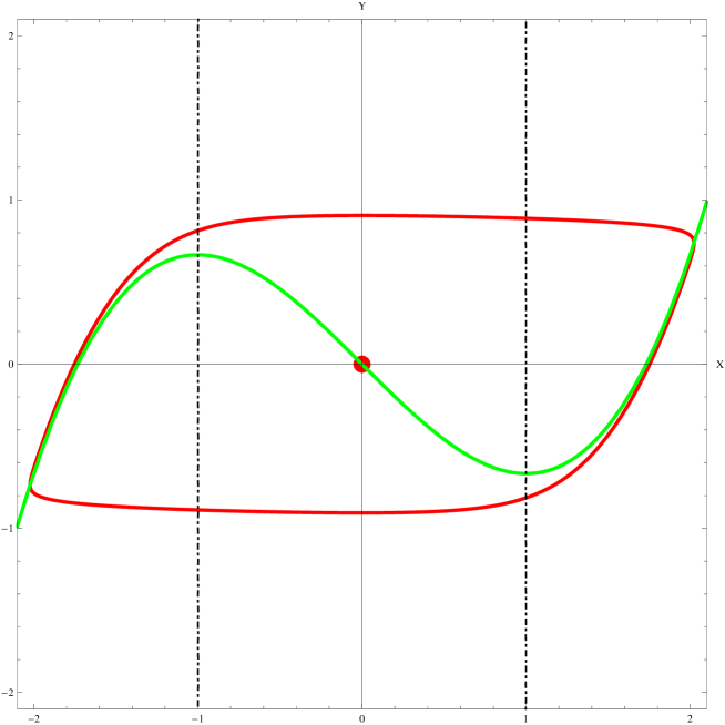
Figure 1. Limit cycle and critical manifold of Van der Pol system (59).

Due to the symmetries of the Van der Pol system (59), let’s focus on the right half part of the $xy$-plane of Fig. 1. It is easy to verify on the one hand that above the critical manifold (in green), $y-F(x)>0$ and, on the other hand that the trajectory curve, i.e. the slow part of the limit cycle is below the critical manifold. It follows that $\dot{x}<0$ in the $\varepsilon$-vicinity of the slow invariant manifold of Van der Pol system (59). Moreover, since $x>0$ in this part of the phase plane, we have $\dot{y}=-x<0$ because $g^{\prime}(x)=1\geqslant 0$. Thus both $x(t)$ and $y(t)$ decrease in this domain as previously stated in Sect. 5. Moreover, according to assumption IV, $F(x)=x^{3}/3-x$ is monotone increasing for $x\geqslant\sqrt{3}$. So $-F(x)$ is monotone decreasing and it has been stated by Lefschetz [31] that “$y(t)$ decreases to the right of the $y$-axis” which implies that $\dot{y}<0$. This leads to $\dot{x}$ decreases in the $\varepsilon$-vicinity of the slow invariant manifold and so $\ddot{x}<0$. Let’s notice that this result is intuitive because the point $M(x(t),y(t))$ of the trajectory curve, integral of the Van der Pol system (59), is then moving on the slow part of the limit cycle. From all these considerations, we deduce that $\ddot{x}\dot{y}>0$. We thus prove that the flow curvature manifold (61) that is to say, a first order approximation in $\varepsilon$ of the slow invariant manifold of Van der Pol singularly perturbed system (59) is positive. Such result could have been directly deduced from Proposition 4 since for Van der Pol system (59), we have $g^{\prime}(x)=1\geqslant 0$.

According to Eq. (27) and since $g^{\prime}(x)=1$, $g^{\prime\prime}(x)=0$, the time derivative of the slow invariant manifold reads for the Van der Pol system (59):

(62) $$\dfrac{d\phi}{dt}=\dddot{x}\dot{y}+\ddot{x}\dot{x}$$

From the Van der Pol system (59) we deduce that:

(63) $$\ddot{x}=\dfrac{1}{\varepsilon}\left[\dot{y}-\left(x^{2}-1\right)\dot{x}\right]=\dfrac{1}{\varepsilon}\left[-x-\left(x^{2}-1\right)\dfrac{1}{\varepsilon}\left[y-F\left(x\right)\right]\right].\\$$

According to assumption IV, $F(x)=x^{3}/3-x$ is monotone increasing for $x\geqslant\sqrt{3}$. So $-F(x)$ is monotone decreasing and it has been stated by Lefschetz [31] that: “ $x(t)$ decreases below the critical manifold and $y(t)$ decreases to the right of the $y$ axis”, it follows that $\ddot{x}$ decreases and so, $\dddot{x}<0$. As a consequence $d\phi/dt>0$. Thus, since we have established that $dE/dt<0$ and $d\phi/dt>0$, in the the $\varepsilon$-vicinity of the slow invariant manifold of Van der Pol system (59), Minorsky’s statement is proved for such system.

7.2. Generalized Liénard singularly perturbed system

According to Llibre et al. [36], an example of generalized Liénard system can be written as follows:

(64) $$\varepsilon\dot{x} =y-\left(\dfrac{x^{5}}{5}+\dfrac{x^{3}}{3}-x\right),$$

$$\dot{y} =-\left(\dfrac{x^{3}}{3}+x\right).$$

Thus we have: $F(x)=\dfrac{x^{5}}{5}+\dfrac{x^{3}}{3}-x$, $f(x)=F^{\prime}(x)=x^{4}+x^{2}-1$, $g(x)=\dfrac{x^{3}}{3}+x$, $g^{\prime}(x)=x^{2}+1$ and $G(x)=\dfrac{x^{4}}{12}+\dfrac{x^{2}}{2}+C$ where we can take $C=0$.

According to (35) we have: $H=x^{2}\left(\dfrac{x^{4}}{18}+\dfrac{x^{2}}{2}+1\right)\leqslant 0$, and according to (57), $\dfrac{dH}{dt}=-4x\left(\dfrac{x^{4}}{12}+\dfrac{x^{2}}{2}\right)\dot{x}\geqslant 0$, because it has been stated that $\dot{x}<0$. From (31), it follows that:

(65) $$\dfrac{dE}{dt}=-\left(x^{4}+x^{2}-1\right)\dot{x}^{2}.$$

The function $x^{4}+x^{2}-1\geqslant 0$ for $x\in]-\infty,-\alpha]\bigcup[+\alpha,+\infty[$ with $\alpha=\sqrt{\dfrac{\sqrt{5}-1}{2}}$ and so, $dE/dt<0$ within this interval which contains the flow curvature manifold that is to say, a first order approximation in $\varepsilon$ of the slow invariant manifold of generalized Liénard singularly perturbed system (64). According to Eq. (22) and since $g^{\prime}(x)=x^{2}+1$, this flow curvature manifold reads:

(66) $$\phi(x,y,\varepsilon)=\ddot{x}\dot{y}+\left(x^{2}+1\right)\dot{x}^{2}.$$

Using the same considerations as previously, it is easy to prove that the flow curvature manifold (66) that is to say, a first order approximation in $\varepsilon$ of the slow invariant manifold of generalized Liénard singularly perturbed system (64) is positive. Such result could have been directly deduced from Proposition 4 since for generalized Liénard system (64), we have $g^{\prime}(x)=x^{2}+1>0$.

According to Eq. (27), the time derivative of the slow invariant manifold reads for generalized Liénard system (64):

(67) $$\dfrac{d\phi}{dt}=\dddot{x}\dot{y}+\dfrac{d}{dt}\left(g^{\prime}(x)\dot{x}\right)$$

Thus from Proposition 5, i.e. since $g^{\prime}(x)=x^{2}+1>0$ and by using the same considerations as previously, it is easy to prove that $d\phi/dt>0$. Therefore since we have established that $dE/dt<0$ and $d\phi/dt>0$, in the the $\varepsilon$-vicinity of the slow invariant manifold of generalized Liénard system (64), Minorsky’s statement is proved for such system.

8. Conclusion

In this work, by using the Flow Curvature Method, we have stated that in the $\varepsilon$-vicinity of the slow invariant manifold of generalized Liénard systems, the curvature of trajectory curve increases while the energy of such systems decreases. Hence we proved Minorsky’s statement for the generalized Liénard systems dating from half a century. Moreover we established a relationship between curvature and energy for such systems that he didn’t provide. Some perspectives to be given to this work should be on the one hand analyze how curvature and energy could be related to the number of limit cycles of such planar singularly dynamical systems. On the other hand, it should be interesting to investigate if these results could be extended to higher dimensional singularly dynamical systems.

It might also be interesting to study the relation between energy considerations and entropy concepts that have been used in the context of slow manifold computation, see e.g. [26, 27], where it has been demonstrated that minimum entropy production and minimum curvature are connected. This seems to be a conceptual analogy of classical thermodynamics with entropy characterizing the degree of energy dissipation.

9. Appendix

Starting from (8) we have the following equation:

$$\varepsilon\ddot{x}+f\left(x\right)\dot{x}+g\left(x\right)=0.$$

By multiplying this equation by $\dot{x}(t)$ and by considering that $f(x)=F^{\prime}(x)$, $g(x)=G^{\prime}(x)$ we obtain:

$$\varepsilon\dot{x}\ddot{x}+\left(F^{\prime}(x)\dot{x}\right)\dot{x}+\left(G^{\prime}(x)\dot{x}\right)=0.$$

Since $\varepsilon\ddot{x}=\dot{y}-F^{\prime}(x)\dot{x}$ we have:

$$\dot{x}\dot{y}+G^{\prime}(x)\dot{x}=0.$$

But $\varepsilon\dot{x}=y-F(x)$, and we find:

$$y\dot{y}+\varepsilon G^{\prime}(x)\dot{x}=F(x)\dot{y}.$$

Finally we obtain:

$$\dfrac{d}{dt}\left(\dfrac{y^{2}}{2}+\varepsilon G(x)\right)=F(x)\dot{y}.$$

Then starting from $y=\varepsilon\dot{x}+F(x)$ we find that:

$$\varepsilon\dfrac{d}{dt}\left(\varepsilon\dfrac{\dot{x}^{2}}{2}+G(x)\right)+\dfrac{d}{dt}\left(\varepsilon F(x)\dot{x}+\dfrac{F^{2}(x)}{2}\right)=F(x)\dot{y}.$$

After simplifications we obtain the following equation:

$$\dfrac{d}{dt}\left(\varepsilon\dfrac{\dot{x}^{2}}{2}+G(x)\right)=-f(x)\dot{x}^{2},$$

which is identical to Eq. (30).

References

- [1] A.A. Andronov & S.E. Chaikin, Theory of Oscillators, I. Moscow, 1937; English transl., Princeton Univ. Press, Princeton, N.J., 1949.
- [2] P. Bergé, Y. Pomeau & Ch. Vidal Order within Chaos. Towards a Deterministic Approach to Turbulence, John Wiley & Sons Ltd., New York, 1987.
- [3] J.D. Cole, Perturbation Methods in Applied Mathematics, Blaisdell, Waltham, MA, 1968.
- [4] G. Darboux, “Sur les éuations différentielles algébriques du premier ordre et du premier degré” Bull. Sci. Math. 2(2) (1878) 60-96, 123-143 & 151-200.
- [5] N. Fenichel, “Persistence and Smoothness of Invariant Manifolds for Flows,” Ind. Univ. Math. J. 21 (1971) 193-225.
- [6] N. Fenichel, “Asymptotic stability with rate conditions,” Ind. Univ. Math. J. 23 (1974) 1109-1137.
- [7] N. Fenichel, “Asymptotic stability with rate conditions II,” Ind. Univ. Math. J. 26 (1977) 81-93.
- [8] N. Fenichel, “Geometric singular perturbation theory for ordinary differential equations” J. Diff. Eq. 31 (1979) 53-98.
- [9] J.M. Ginoux & B. Rossetto, “Differential geometry and mechanics applications to chaotic dynamical systems,” International Journal of Bifurcation & Chaos 4(16) (2006) 887-910.
- [10] J.M. Ginoux, B. Rossetto & L.O. Chua, “Slow invariant manifolds as curvature of the flow of dynamical systems,” International Journal of Bifurcation & Chaos 11(18) (2008) 3409-3430.
- [11] J.M. Ginoux, Differential geometry applied to dynamical systems, World Scientific Series on Nonlinear Science, Series A 66 (World Scientific, Singapore), 2009.
- [12] J.M. Ginoux & J. Llibre, “Flow curvature method applied to canard explosion,” Journal of Physics A: Mathematical and Theoretical, 44 (46), 465203 (2011).
- [13] J.M. Ginoux, J. Llibre & L.O. Chua, “Canards from Chua’s circuit,” International Journal of Bifurcation & Chaos, 23(4), 1330010 (2013) [13 pages].
- [14] J.M. Ginoux “The Slow Invariant Manifold of the Lorenz-Krishnamurthy Model,” Qualitative Theory of Dynamical Systems, 13(1), (2014), 19-37.
- [15] J.M. Ginoux & J. Llibre, “Canards Existence in FitzHugh-Nagumo and Hodgkin-Huxley Neuronal Models,” Mathematical Problems in Engineering, December 2015(2), Article ID 342010 (17 pages),
- [16] J.M. Ginoux & J. Llibre, “Canards Existence in Memristor’s Circuits,” Qualitative Theory of Dynamical Systems, 15(2), (October 2016), 383-431.
- [17] J.M. Ginoux History of nonlinear oscillations theory, Archimede, New Studies in the History and Philosophy of Science and Technology, vol. 49, Springer, (New York), 2017.
- [18] J.M. Ginoux, J. Llibre & K. Tchizawa, “Canards Existence in The Hindmarsh-Rose Model,” Mathematical Modelling of Natural Phenomena, Vol. 14 (4), (12 July 2019), 1-21.
- [19] J.M. Ginoux, Differential geometry applied to dynamical systems, World Scientific Series on Nonlinear Science, Series A 66 (World Scientific, Singapore), 2009.
-
[20]
R. Gilmore, J.M. Ginoux, T. Jones, C Letellier & U. S. Freitas,
“Connecting curves for dynamical systems,” J. Phys. A: Math. Theor., 43 (2010) 255101 (13pp). - [21] P. Heiter & D. Lebiedz “Towards differential geometric characterization of slow invariant manifolds in extended phase space: Sectional curvature and flow invariance”, SIAM J. Appl. Dyn. Syst. 17(1) (2018), 732-753.
- [22] M. W. Hirsch, C.C. Pugh & M. Shub, Invariant Manifolds, Springer-Verlag, New York, 1977.
- [23] C.K.R.T. Jones, Geometric Singular Pertubation Theory, in Dynamical Systems, Montecatini Terme, L. Arnold, Lecture Notes in Mathematics, vol. 1609, Springer-Verlag, 1994, pp. 44-118.
- [24] T. Kaper, “An Introduction to Geometric Methods and Dynamical Systems Theory for Singular Perturbation Problems,” in Analyzing multiscale phenomena using singular perturbation methods, (Baltimore, MD, 1998), pages 85-131. Amer. Math. Soc., Providence, RI, 1999.
- [25] M. Krupa & P. Szmolyan, “Relaxation Oscillation and Canard Explosion,” J. Diff. Eq. 174 (2001) 312-368.
- [26] D. Lebiedz, “Computing minimal entropy production trajectories: An approach to model reduction in chemical kinetics”, J. Chem. Phys. 120(5) (2004), 6890-6897.
- [27] D. Lebiedz, “Entropy-related extremum principles for model reduction of dissipative dynamical systems”, Entropy 12(4) (2010), 706-719.
- [28] D. Lebiedz, V. Reinhardt & J. Siehr “Minimal curvature trajectories: Riemannian geometry concepts for slow manifold computation in chemical kinetics”, J. Comput. Phys. 229(18) (2010), 6512-6533
- [29] D. Lebiedz & J. Siehr “A continuation method for efficient solution of parametric optimization problems in kinetic model reduction,” SIAM J. Sci. Comput. 33(2) (2011), 703-720.
- [30] D. Lebiedz, J. Siehr & J. Unger “A variational principle for computing slow invariant manifolds in dissipative dynamical systems”, SIAM J. Sci. Comput. 35(3) (2013), A1584-A1603.
- [31] S. Lefschetz Differential equations: Geometric theory, Interscience Publishers, John Wiley and Sons, New York, New York 1957.
- [32] N. Levinson & O. K. Smith “A general equation for relaxation oscillations,” Duke Mathematical Journal, 9 (1942), 382-403.
- [33] N. Levinson, “A Second order differential equation with singular solutions,” Ann. Math. 50 (1949) 127-153.
- [34] A. Liénard “Étude des oscillations entretenues,” Revue Générale de l’Électricité, 23, (1928), 901-912 and 946-954.
- [35] J. Llibre & J.C. Medrado, “On the invariant hyperplanes for d-dimensional polynomial vector fields” J. Phys. A: Math. Theor. 40 (2007) 8385-8391.
- [36] J. Llibre, A.C. Mereu & M.A. Teixeira “Limit cycles of the generalized polynomial Liénard differential equations,” Math. Proc. Cambridge Philos. Soc. 148 (2010) 363-383.
- [37] R.E. O’Malley, Introduction to Singular Perturbations, Academic Press, New York, 1974.
- [38] R.E. O’Malley, Singular Perturbations Methods for Ordinary Differential Equations, Springer-Verlag, New York, 1991.
- [39] N. Minorsky, Théorie des oscillations, Mémorial des sciences mathématiques, fascicule 163, 1967.
- [40] L. Perko Differential Equations and Dynamical Systems, Texts in Applied Mathematics, Volume 7, Springer-Verlag New York, 2001.
- [41] D. Schlomiuk, “Elementary first integrals of differential equations and invariant algebraic curves,” Expositiones Mathematicae 11 (1993) 433-454.
- [42] Szmolyan, M. Wechselberger, “Canards in ,” J. Diff. Eq. 177 (2001) 419-453.
- [43] F. Takens, “Constrained equations; A study of implicit differential equations and their discontinuous solutions,” in Lecture Notes in Mathematics volume 525 (1976), Springer Verlag.
- [44] A.N. Tikhonov, “On the dependence of solutions of differential equations on a small parameter,” Mat. Sbornik N.S., 31 (1948) 575-586.
- [45] B. Van der Pol, On “relaxation-oscillations”, The London, Edinburgh, and Dublin Philosophical Magazine and Journal of Science, (VII), 2 978-992 (1926).
- [46] W.R. Wasow, Asymptotic Expansions for Ordinary Differential Equations, Wiley-Interscience, New York, 1965.