PTOPO: Computing the Geometry and the Topology of Parametric Curves

Abstract

We consider the problem of computing the topology and describing the geometry of a parametric curve in $\mathbb{R}^{n}$. We present an algorithm, PTOPO, that constructs an abstract graph that is isotopic to the curve in the embedding space. Our method exploits the benefits of the parametric representation and does not resort to implicitization.

Most importantly, we perform all computations in the parameter space and not in the implicit space. When the parametrization involves polynomials of degree at most $d$ and maximum bitsize of coefficients $\tau$, then the worst case bit complexity of PTOPO is $\widetilde{\mathcal{O}}_{B}(nd^{6}+nd^{5}\tau+d^{4}(n^{2}+n\tau)+d^{3}(n^{2}\tau+n^{3})+n^{3}d^{2}\tau)$. This bound matches the current record bound $\widetilde{\mathcal{O}}_{B}(d^{6}+d^{5}\tau)$ for the problem of computing the topology of a plane algebraic curve given in implicit form. For plane and space curves, if $N=\max\{d,\tau\}$, the complexity of PTOPO becomes $\widetilde{\mathcal{O}}_{B}(N^{6})$, which improves the state-of-the-art result, due to Alcázar and Díaz-Toca [CAGD’10], by a factor of $N^{10}$. In the same time complexity, we obtain a graph whose straight-line embedding is isotopic to the curve. However, visualizing the curve on top of the abstract graph construction, increases the bound to $\widetilde{\mathcal{O}}_{B}(N^{7})$. For curves of general dimension, we can also distinguish between ordinary and non-ordinary real singularities and determine their multiplicities in the same expected complexity of PTOPO by employing the algorithm of Blasco and Pérez-Díaz [CAGD’19]. We have implemented PTOPO in maple for the case of plane and space curves. Our experiments illustrate its practical nature.

1 Introduction

Parametric curves constitute a classical and important topic in computational algebra and geometry (Sendra and Winkler, 1999) that constantly receives attention, e.g.,  (Sederberg, 1986; Cox et al., 2011; Busé et al., 2019; Sendra et al., 2008). The motivation behind the continuous interest in efficient algorithms for computing with parametric curves emanates, among others reasons, by the frequent presence of parametric representations in computer modeling and computer aided geometric design, e.g., (Farouki et al., 2010).

We focus on computing the topology of a real parametric curve, that is, the computation of an abstract graph that is isotopic (Boissonnat and Teillaud, 2006, p. 184) to the curve in the embedding space. We design an algorithm, PTOPO, that applies directly to rational parametric curves of any dimension and is complete, in the sense that there are no assumptions on the input. We consider different characteristics of the parametrization, like properness and normality, before computing the singularities and other interesting points on the curve. These points are necessary for representing the geometry of the curve, as well as for producing a certified visualization of plane and space curves.

Previous work

A common strategy when dealing with parametric curves is implicitization. There has been a lot of research effort, e.g., Sederberg and Chen (1995); Busé et al. (2019) and the references therein, in designing algorithms to compute the implicit equations describing the curve. However, it is also important to manipulate parametric curves directly, without converting them to implicit form. For example, in the parametric form it is easier to visualize the curve and to find points on it. The advantages of the latter become more significant for curves of high dimension.

The study of the topology of a real parametric curve is a topic that has not received much attention in the literature, in contrast to its implicit counterpart (Diatta et al., 2018; Kobel and Sagraloff, 2014). The computation of the topology requires special treatment, since for instance it is not always easy to choose a parameter interval such that when we plot the curve over it, we include all the important topological features (like singular and extreme points) (Alcázar and Díaz-Toca, 2010). Moreover, while visualizing the curve using symbolic computational tools, the problem of missing points and branches may arise (Recio, 2007; Sendra, 2002). Alcázar and Díaz-Toca (2010) study the topology of real parametric curves without implicitizing. They work directly with the parametrization and address both plane and space real rational curves. Our algorithm to compute the topology is to be juxtaposed to their work. We also refer to Caravantes et al. (2014) and Alberti et al. (2008) for other approaches based on computations by values and subdivision, respectively.

To compute the topology of a curve it is essential to detect its singularities. This is an important and well studied problem (Alcázar and Díaz-Toca, 2010; Rubio et al., 2009; Kobel and Sagraloff, 2014) of independent interest. To identify the singularities, we can first compute the implicit representation and then apply classical approaches (Walker, 1978; Fulton, 1969). Alternatively, we can compute the singularities using directly the parametrization. For instance, there are necessary and sufficient conditions to identify cusps and inflection points using determinants, e.g., (Li and Cripps, 1997; Manocha and Canny, 1992).

On computing the singularities of a parametric curve, a line of work related to our approach, does so by means of a univariate resultant (Abhyankar and Bajaj, 1989; van den Essen and YU, 1997; Park, 2002; Pérez-Díaz, 2007; Gutierrez et al., 2002a). We can use the Taylor resultant (Abhyankar and Bajaj, 1989) and the $D$-resultant (van den Essen and YU, 1997) of two polynomials in $K[t]$, to find singularities of plane curves parametrized by polynomials, where $K$ is a field of characteristic zero in the first case and of arbitrary characteristic in the latter, without resorting to the implicit form. Park (2002) extends previous results to curves parametrized by polynomials in affine $n$-space. The generalization of the $D$-resultant for a pair of rational functions and its application to the study of rational plane curves, is due to Gutierrez et al. (2002a). In (Pérez-Díaz, 2007; Blasco and Pérez-Díaz, 2019) they present a method for computing the singularities of plane curves using a univariate resultant and characterizing the singularities using its factorization. Notably Rubio et al. (2009) work on rational parametric curves in affine $n$-space; they use generalized resultants to find the parameters of the singular points. Moreover, they characterize the singularities and compute their multiplicities.

Cox et al. (2011) use the syzygies of the ideal generated by the polynomials that give the parametrization to compute the singularities and their structure. There are state-of-the-art approaches that exploit this idea and relate the problem of computing the singularities with the notion of the $\mu$-basis of the parametrization, e.g., (Jia et al., 2018) and references therein. Chionh and Sederberg (2001) reveal the connection between the implicitization Bézout matrix and the singularities of a parametric curve. Busé and D’Andrea (2012) present a complete factorization of the invariant factors of resultant matrices built from birational parametrizations of rational plane curves in terms of the singular points of the curve and their multiplicity graph. Let us also mention the important work on matrix methods (Busé, 2014; Busé and Luu Ba, 2010) for representing the implicit form of parametric curves, that is suitable for numerical computations. Bernardi et al. (2016) use the projection from the rational normal curve to the curve and exploit secant varieties.

Overview of our approach and our contributions

We introduce PTOPO, a complete, exact, and efficient algorithm (Alg. 3) for computing the geometric properties and the topology of rational parametric curves in $\mathbb{R}^{n}$. Unlike other algorithms, e.g. Alcázar and Díaz-Toca (2010), it makes no assumptions on the input curves, such as the absence of axis-parallel asymptotes, and is applicable to any dimension. Nevertheless, it does not identify knots for space curves nor it can be used for determining the equivalence of two knots.

If the (proper) parametrization of the curve consists of polynomials of degree $d$ and bitsize $\tau$, then PTOPO outputs a graph isotopic (Boissonnat and Teillaud, 2006, p.184), Alcázar et al. (2020) to the curve in the embedding space, by performing

$$\widetilde{\mathcal{O}}_{B}(nd^{6}+nd^{5}\tau+d^{4}(n^{2}+n\tau)+d^{3}(n^{2}\tau+n^{3})+n^{3}d^{2}\tau)$$

bit operations in the worst case (Thm. 24), assuming no singularities at infinity. We also provide a Las Vegas variant with expected complexity

$$\widetilde{\mathcal{O}}_{B}(d^{6}+d^{5}(n+\tau)+d^{4}(n^{2}+n\tau)+d^{3}(n^{2}\tau+n^{3})+n^{3}d^{2}\tau).$$

If $n=\mathcal{O}(1)$, the bounds become $\widetilde{\mathcal{O}}_{B}(N^{6})$, where $N=\max\{d,\tau\}$. The vertices of the output graph correspond to special points on the curve, in whose neighborhood the topology is not trivial, given by their parameter values. Each edge of the graph is associated with two parameter values and corresponds to a unique smooth parametric arc. For an embedding isotopic to the curve, we map every edge of the abstract graph to the corresponding parametric arc.

For plane and space curves, our bound improves the previously known bound due to Alcázar and Díaz-Toca (2010) by a factor of $\widetilde{\mathcal{O}}_{B}(N^{10})$. The latter algorithm (Alcázar and Díaz-Toca, 2010) performs some computations in the implicit space. On the contrary, PTOPO is a fundamentally different approach since we work exclusively in the parameter space and we do not use a sweep-line algorithm to construct the isotopic graph. We handle only the parameters that give important points on the curve, and thus, we avoid performing operations such as univariate root isolation in an extension field or evaluation of a polynomial at an algebraic number.

Computing singular points is an essential part of PTOPO (Lem. 18). We chose not to exploit recent methods, e.g., (Blasco and Pérez-Díaz, 2019), for this task because this would require introducing new variables (to employ the T-resultant). We employ older techniques, e.g., (Rubio et al., 2009; Pérez-Díaz, 2007; Alcázar and Díaz-Toca, 2010), that rely on a bivariate polynomial system, Eq. (2). We take advantage of this system’s symmetry and of nearly optimal algorithms for bivariate system solving and for computations with real algebraic numbers (Diatta et al., 2018; Bouzidi et al., 2016; Diochnos et al., 2009; Pan and Tsigaridas, 2017). In particular, we introduce an algorithm for isolating the roots of over-determined bivariate polynomial systems by exploiting the Rational Univariate Representation (RUR) (Bouzidi et al., 2015b, 2016, 2013) that has worst case and expected bit complexity that matches the bounds for square systems (Thm. 16). These are key steps for obtaining the complexity bounds of Thm. 23 and Thm. 24.

Moreover, our bound matches the current state-of-the-art complexity bound, $\widetilde{\mathcal{O}}_{B}(d^{6}+d^{5}\tau)$ or $\widetilde{\mathcal{O}}_{B}(N^{6})$, for computing the topology of implicit plane curves Diatta et al. (2018); Kobel and Sagraloff (2014). However, if we want to visualize the graph in 2D or 3D, then we have to compute a characteristic box (Lem. 20) that contains all the the topological features of the curve and the intersections of the curve with its boundary. In this case, the complexity of PTOPO becomes $\widetilde{\mathcal{O}}_{B}(N^{7})$ (Thm. 23).

A preprocessing step of PTOPO consists of finding a proper reparametrization of the curve (if it is not proper). We present explicit bit complexity bounds (Lem. 6) for the algorithm of Pérez-Díaz (2006) to compute a proper parametrization. Another preprocessing step is to ensure that there are no singularities at infinity. Lem. 7 handles this task and provides explicit complexity estimates.

Additionally, we consider the case where the embedding of the abstract graph has straight line edges and not parametric arcs; in particular for plane curves, we show that the straight line embedding of the abstract graph in $\mathbb{R}^{2}$ is already isotopic to the curve (Cor. 26). For space curves, the procedure supported by Thm. 28 adds a few extra vertices to the abstract graph, so that the straight line embedding in $\mathbb{R}^{3}$ is isotopic to the curve. The extra number of vertices serves in resolving situations where self-crossings occur when continuously deforming the graph to the curve. In Thm. 30 we also prove that for curves of any dimension, we can compute the multiplicities and the characterization of singular points in the same bit-complexity as computing the points (in a Las Vegas setting). For that, we use the method by Blasco and Pérez-Díaz (2019), which does not require any further computations apart from solving the system that gives the parameters of the singular points (cf. Alcázar and Díaz-Toca (2010)).

Last but not least, we provide a certified implementation of PTOPO in maple. The implementation computes the topology of plane and space curves and visualizes them. If the input consists of rational polynomials, our algorithm and the implementation is certified, since, first of all, the algorithm always outputs the correct geometric and topological result. This is because we perform exact computations with real algebraic numbers based on arithmetic over the rationals. Moreover, no assumption that cannot be verified (for example by another algorithm) is made on the input.

A preliminary version of our work appeared in Katsamaki et al. (2020a). Compared with this version, we add all the missing proofs for the algebraic tools that we use in our algorithm, we present the isotopic embedding for plane and space curves (Sec. 6), and analyze the complexity of the algorithm of Blasco and Pérez-Díaz (2019) to determine the multiplicities and the character of real singular points (Sec. 7).

Organization of the paper

The next section presents our notation and some useful results needed for our proofs. In Sec. 3 we give the basic background on rational curves in affine $n$-space. We characterize the parametrization by means of injectivity and surjectivity and describe a reparametrization algorithm. In Sec. 4 we present the algorithm to compute the singular, extreme points (in the coordinate directions), and isolated points on the curve. In Sec. 5 we describe our main algorithm, PTOPO, that constructs a graph isotopic to the curve in the embedding space and its complexity. In Sec. 6 we expatiate on the isotopic embedding for plane and space curves. In Sec. 7, we study the multiplicities and the character of real singular points for curves of arbitrary dimension. Finally, in Sec. 8 we give examples and experimental results.

2 Notation and Algebraic Tools

For a polynomial $f\in\mathbb{Z}[X]$, its infinity norm is equal to the maximum absolute value of its coefficients. We denote by $\mathcal{L}(f)$ the logarithm of its infinity norm. We also call the latter the bitsize of the polynomial. A univariate polynomial is of size $(d,\tau)$ when its degree is at most $d$ and has bitsize $\tau$. The bitsize of a rational function is the maximum of the bitsizes of the numerator and the denominator. We represent an algebraic number $\alpha\in\mathbb{C}$ by the isolating interval representation. When $\alpha\in\mathbb{R}$ (resp. $\mathbb{C}$), it includes a square-free polynomial which vanishes at $\alpha$ and a rational interval (resp. Cartesian products of rational intervals) containing $\alpha$ and no other root of this polynomial (see for example (Yap, 1999)). We denote by $\mathcal{O}$ (resp. $\mathcal{O}_{B}$) the arithmetic (resp. bit) complexity and we use $\widetilde{\mathcal{O}}$ (resp. $\widetilde{\mathcal{O}}_{B}$) to ignore (poly-)logarithmic factors. We denote the resultant of the polynomials $f,g$ with respect to $x$ by $\mathtt{res}_{x}(f,g)$ . For $t\in\mathbb{C}$, we denote by $\bar{t}$ its complex conjugate. We use $[n]$ to signify the set $\{1,\dots,n\}$.

We now present some useful results, needed for our analysis.

Lemma 1.

Let $A=\sum_{i=0}^{m}a_{i}X^{i},B=\sum_{i=0}^{n}b_{i}X^{i}\in\mathbb{Z}[X]$ of degrees $m$ and $n$ and of bitsizes $\tau$ and $\sigma$ respectively. Let $\alpha_{1},\dots,\alpha_{m}$ be the complex roots of $A$, counting multiplicities. Then, for any $\kappa=1,\dots,m$ it holds that

$$2^{-m\sigma-n\tau-(m+n)\log(m+n)}<|B(\alpha_{\kappa})|<2^{m\sigma+n\tau+(m+n)\log(m+n)}.$$

Proof.

Following Strzebonski and Tsigaridas (2019), let $R=\mathtt{res}_{X}(A(X),Y-B(X))\in\mathbb{Z}[Y]$. Using the Poisson’s formula for the resultant we can write $R(Y)=a_{m}^{n}\prod_{\kappa=1}^{m}(Y-B(\alpha_{\kappa}))$. The maximum bitsize of the coefficients of $R(Y)$ is at most $m\sigma+n\tau+(m+n)\log(m+n)$. We observe that the roots of $R(Y)$ are $B(\alpha_{\kappa})$ for $\kappa=1,\dots,m$. Therefore, using Cauchy’s bound we deduce that

$$2^{-m\sigma-n\tau-(m+n)\log(m+n)}<|B(\alpha_{\kappa})|<2^{m\sigma+n\tau+(m+n)\log(m+n)}.$$

∎

Lemmata  2 and 3 restate known results on the gcd computation of various univariate and bivariate polynomials.

Lemma 2.

Let $f_{1}(X),\dots,f_{n}(X)\in\mathbb{Z}[X]$ of sizes $(d,\tau)$. We can compute their $\gcd$, which is of size $(d,\widetilde{\mathcal{O}}(d+\tau))$, in worst case complexity $\widetilde{\mathcal{O}}_{B}(n(d^{3}+d^{2}\tau))$, with a Monte Carlo algorithm in $\widetilde{\mathcal{O}}_{B}(d^{2}+d\tau)$, or with a Las Vegas algorithm in $\widetilde{\mathcal{O}}_{B}(n(d^{2}+d\tau))$.

Proof.

These are known results (von zur Gathen and Gerhard, 2013). We repeat the arguments adapted to our notation.

Worst case: We compute $g$ by performing $n$ consecutive $\gcd$ computations, that is

$$\gcd(f_{1},\gcd(f_{2},\gcd(\cdots,\gcd(f_{n-1},f_{n}))).$$

Since each $\gcd$ computation costs $\widetilde{\mathcal{O}}_{B}(d^{3}+d^{2}\tau)$ (Bouzidi et al., 2015b, Lem.4), the result for this case follows.

Monte Carlo: We perform one gcd computation by allowing randomization. If we choose integers $a_{3},\dots,a_{n}$ independently at random from the set $\{1,\dots,Kd\}$, where $K=\mathcal{O}(1)$, we get that $\gcd(f_{1},\dots,f_{n})=\gcd(f_{1},f_{2}+a_{3}f_{3}+\dots+a_{n}f_{n})$ in $\mathbb{Z}[x]$, with probability $\geq 1/2$ (von zur Gathen and Gerhard, 2013, Thm. 6.46). This actually computes the monic gcd in $\mathbb{Q}$. To compute the gcd in $\mathbb{Z}$ we need to multiply with the gcd of the leading coefficients of $f_{1},f_{2}+a_{3}f_{3}+\dots+a_{n}f_{n}$ and then take the primitive part of the resulting polynomial. This is sufficient since the leading coefficient of the gcd in $\mathbb{Z}[X]$ divides the leading coefficients of the two polynomials. Also, by (von zur Gathen and Gerhard, 2013, Cor. 6.10) the monic gcd of two polynomials in $\mathbb{Q}[X]$ is equal to their gcd in $\mathbb{Z}[X]$ divided by their leading coefficient. The gcd of the two leading coefficients of $f_{1},f_{2}+a_{3}f_{3}+\dots+a_{n}f_{n}$ is an integer of bitsize $\widetilde{\mathcal{O}}(\tau)$, therefore this does not pollute the total complexity.

We compute $g^{*}=\gcd(f_{1},f_{2}+a_{3}f_{3}+\dots+a_{n}f_{n})$. Notice that the polynomial $f_{2}+a_{3}f_{3}+\dots+a_{n}f_{n}$ is asymptotically of size $(d,\tau)$. So, it takes $\widetilde{\mathcal{O}}_{B}(d^{2}+d\tau)$ to find $g^{*}$, using the probabilistic algorithm in Schönhage (1988).

Las Vegas: We can reduce the probability of failure in the Monte Carlo variant of the $\gcd$ computation to zero, by performing $n$ exact divisions. In particular, we check if $g^{*}$ divides $f_{3},\dots,f_{n}$. Using (von zur Gathen and Gerhard, 2013, Ex.10.21), the bit complexity of these operations is in total $\widetilde{\mathcal{O}}_{B}(n(d^{2}+d\tau))$. ∎

Lemma 3.

Let $f_{1}(X,Y),\dots,f_{n}(X,Y)\in\mathbb{Z}[X,Y]$ of bidegrees $(d,d)$ and $\mathcal{L}(f_{i})=\tau$. We can compute their $\gcd$, which is of bitsize $\widetilde{\mathcal{O}}(d+\tau)$, in worst case complexity $\widetilde{\mathcal{O}}_{B}(n(d^{5}+d^{4}\tau))$, with a Monte Carlo algorithm in $\widetilde{\mathcal{O}}_{B}(d^{3}+d^{2}\tau)$, or with a Las Vegas algorithm in $\widetilde{\mathcal{O}}_{B}(n(d^{3}+d^{2}\tau))$.

Proof.

The straightforward approach is to perform $n$ consecutive $\gcd$ computations, that is

$$\gcd(f_{1},\gcd(f_{2},\gcd(\cdots,\gcd(f_{n-1},f_{n}))).$$

To accelerate the practical complexity we sort $f_{i}$ in increasing order with respect to their degree. Each $\gcd$ computation costs $\widetilde{\mathcal{O}}_{B}(d^{5}+d^{4}\tau)$ (Bouzidi et al., 2016, Lem. 5), so the total worst case cost is $\widetilde{\mathcal{O}}_{B}(nd^{5}+nd^{4}\tau)$.

Alternatively, we consider the operation $\gcd(f_{1},\sum_{k=2}^{n}{a_{k}f_{k}})$, where $a_{k}$ are random integers, following (von zur Gathen and Gerhard, 2013, Thm. 6.46). The expected cost of this gcd is $\widetilde{\mathcal{O}}_{B}(d^{3}+d^{2}\tau)$. To see this, notice that we can perform a bivariate $\gcd$ in expected time $\widetilde{\mathcal{O}}(d^{2})$ (von zur Gathen and Gerhard, 2013, Cor. 11.12), over a finite field with enough elements, and the bitsize of the result is $\widetilde{\mathcal{O}}(d+\tau)$ Mahler (1962).

Then, for a Las Vegas algorithm, using exact division, we test if the resulting polynomial divides all $f_{i}$, for $2\leq i\leq n$. This costs $\widetilde{\mathcal{O}}_{B}(n(d^{3}+d^{2}\tau))$, by adapting (von zur Gathen and Gerhard, 2013, Ex.10.21) to the bivariate case. ∎

3 Rational curves

Following Alcázar and Díaz-Toca (2010) closely, we introduce basic notions for rational curves. Let $\widetilde{\mathcal{C}}$ be an algebraic curve over $\mathbb{C}^{n}$, parametrized by the map

$$\phi: \quad\mathbb{C}\dashrightarrow\widetilde{\mathcal{C}}$$

$$\quad t\mapsto\big{(}\phi_{1}(t),\dots,\phi_{n}(t)\big{)}=\Big{(}\frac{p_{1}(t)}{q_{1}(t)},\dots,\frac{p_{n}(t)}{q_{n}(t)}\Big{)},$$ (1)

where $p_{i},q_{i}\in\mathbb{Z}[t]$ are of size $(d,\tau)$ for $i\in[n]$, and $\widetilde{\mathcal{C}}$ is the Zariski closure of ${\text{Im}(\phi)}$. We call $\phi(t)$ a parametrization of $\widetilde{\mathcal{C}}$.

We study the real trace of $\tilde{\mathcal{C}}$, that is $\mathcal{C}:=\tilde{\mathcal{C}}\cap\mathbb{R}^{n}$. A parametrization $\phi$ is chatacterized by means of properness (Sec. 3.1) and normality (Sec. 3.2). To ensure these properties, one can reparametrize the curve, i.e., apply a rational change of parameter to the given parametrization. We refer to (Sendra et al., 2008, Ch. 6) for more details on reparametrization.

Without loss of generality, we assume that no coordinate of the parametrization $\phi$ is constant; otherwise we could embed $\tilde{\mathcal{C}}$ in a lower dimensional space. We consider that $\phi$ is in reduced form, i.e., $\gcd(p_{i}(t),q_{i}(t))=1$, for all $i\in[n]$. The point at infinity, $\mathbf{p}_{\infty}$, is the point on $\mathcal{C}$ we obtain for $t\rightarrow\pm\infty$ (if it exists). For a parametrization $\phi$, we consider the following system of bivariate polynomials:

$$h_{i}(s,t)=\frac{p_{i}(s)q_{i}(t)-q_{i}(s)p_{i}(t)}{s-t},\quad\text{ for }i\in[n].$$ (2)

Remark 4.

For every $i\in[n]$ $h_{i}(s,t)$ is a polynomial since $(s,s)$ is a root of the numerator for every $s$. Also, $h_{i}(t,t)=\phi^{\prime}_{i}(t)q_{i}^{2}(t)$ (Gutierrez et al., 2002b, Lem. 1.7).

3.1 Proper parametrization

A parametrization is proper if $\phi(t)$ is injective for almost all points on $\widetilde{\mathcal{C}}$. In other words, almost every point on $\widetilde{\mathcal{C}}$ is the image of exactly one parameter value (real or complex). For other equivalent definitions of properness, we refer the reader to (Sendra et al., 2008, Ch. 4), (Rubio et al., 2009). As stated in (Alcázar and Díaz-Toca, 2010, Thm. 1), a parametrization is proper if and only if $\deg(\gcd(h_{1}(s,t),\dots,h_{n}(s,t)))=0$. This leads to an algorithm for checking properness. By applying Lem. 3 we get the following:

Lemma 5.

There is an algorithm that checks if a parametrization $\phi$ is proper in worst-case bit complexity $\widetilde{\mathcal{O}}_{B}(n(d^{5}+d^{4}\tau))$ and in expected bit complexity $\widetilde{\mathcal{O}}_{B}(n(d^{3}+d^{2}\tau))$.

Proof.

We construct the polynomials $h_{i}(s,t)$ for all $i\in[n]$ in $\mathcal{O}_{B}(nd^{2}\tau)$. Then, we need to check if $\deg(\gcd(h_{1}(s,t),\dots,h_{n}(s,t)))=0$ (Alcázar and Díaz-Toca, 2010, Thm. 1). For the $\gcd$ computation, we employ Lem. 3 and the result follows. ∎

If $\phi$ is a not a proper parametrization, then there always exists a parametrization $\psi\in\mathbb{Z}(t)^{n}$ and $R(t)\in\mathbb{Z}(t)$ such that $\psi(R(t))=\phi(t)$ and $\psi$ is proper (Sendra et al., 2008, Thm. 7.6). There are various algorithms for obtaining a proper parametrization, e.g., (Sederberg, 1986; Gutierrez et al., 2002a; Sendra et al., 2008; Pérez-Díaz, 2006; Gao and Chou, 1992). We consider the algorithm in (Pérez-Díaz, 2006) for its simplicity; its pseudo-code is in Alg. 1.

Input: A parametrization $\phi\in\mathbb{Z}(t)^{n}$ as in Eq. (1)

1

Output: A proper parametrization $\psi=(\psi_{1},\dots,\psi_{n})\in\mathbb{Z}(t)^{n}$

2

3for $i\in[n]$  do  $H_{i}(s,t)\leftarrow p_{i}(s)q_{i}(t)-p_{i}(t)q_{i}(s)\in\mathbb{Z}[s,t]$ ;

4

5$H\leftarrow\gcd(H_{1},\dots,H_{n})=C_{m}(t)s^{m}+\cdots+C_{0}(t)\in(\mathbb{Z}[t])[s]$

6if  $m=1$ then return $\phi(t)$ ;

7

8Find $k,l\in[m]$ such that:
$\deg(\gcd(C_{k}(t),C_{l}(t)))=0$ and $\frac{C_{k}(t)}{C_{l}(t)}\not\in\mathbb{Q}$

9$R(t)\leftarrow\frac{C_{k}(t)}{C_{l}(t)}$

10$r\leftarrow\deg(R)=\max\{\deg(C_{k}),\deg(C_{l})\}$

11$G\leftarrow s\,C_{l}(t)-C_{k}(t)$

12for $i\in[n]$ do

13       $F_{i}\leftarrow xq_{i}(t)-p_{i}(t)$

14      $L_{i}(s,x)\leftarrow\mathtt{res}_{t}(F_{i}(t,x),G(t,s))=(\tilde{q}_{i}(s)x-\tilde{p}_{i}(s))^{r}$

15

return $\psi(t)=\big{(}\frac{\tilde{p}_{1}(t)}{\tilde{q}_{1}(t)},\dots,\frac{\tilde{p}_{n}(t)}{\tilde{q}_{n}(t)}\big{)}$

Algorithm 1 Make_Proper($\phi$)

Lemma 6.

Consider a non-proper parametrization of a curve $\mathcal{C}$, consisting of univariate polynomials of size $(d,\tau)$. Alg. 1 computes a proper parametrization of $\mathcal{C}$, involving polynomials of degree at most $d$ and bitsize $\mathcal{O}(d^{2}+d\tau)$, in $\widetilde{\mathcal{O}}_{B}(n(d^{5}+d^{4}\tau))$, in the worst case.

Proof.

The correctness of the algorithm is proved in (Pérez-Díaz, 2006). We analyze its complexity. The algorithm first computes the bivariate polynomials $H_{i}(s,t)=p_{i}(s)q_{i}(t)-p_{i}(t)q_{i}(s)$ for $i=1,\dots,n$. They have bi-degree at most $(d,d)$ and bitsize at most $2\tau+1$. Then, we compute their $\gcd$, which we denote by $H$, in $\widetilde{\mathcal{O}}_{B}(n(d^{5}+d^{4}\tau))$ (Lem. 3). By (Mahler, 1962) and (Basu et al., 2003, Prop. 10.12) we have that $\mathcal{L}(H)=\mathcal{O}(d+\tau)$. If we write $H=C_{m}(t)s^{m}+\cdots+C_{0}(t)$, it also holds that $\mathcal{L}(C_{j})=\mathcal{O}(d+\tau)$, $j=1,\dots,m$.

If the degree of $H$ is one, then the parametrization is already proper and we have nothing to do. Otherwise, we consider $H$ as a univariate polynomial in $s$ and we find two of its coefficients that are relatively prime, using exact division. The complexity of this operation is $m^{2}\times\widetilde{\mathcal{O}}_{B}(d^{2}+d\tau)=\widetilde{\mathcal{O}}_{B}(d^{4}+d^{3}\tau)$ (von zur Gathen and Gerhard, 2013, Ex. 10.21).

Subsequently, we perform $n$ resultant computations to get $L_{1},\dots L_{n}$, as defined in Alg. 1. From these we obtain the rational functions of the new parametrization. We focus on the computation of $L_{1}$. The same arguments hold for all $L_{i}$. The bi-degree of $L_{1}(s,x)$ is $(d,d)$ (Basu et al., 2003, Prop. 8.49) and $\mathcal{L}(L_{1})=\mathcal{O}(d^{2}+d\tau)$ (Basu et al., 2003, Prop. 8.50); the latter dictates the bitsize of the new parametrization.

To compute $L_{1}$, we consider $F_{1}$ and $G$ as univariate polynomials in $t$ and we apply a fast algorithm for computing the univariate resultant based on subresultants (Lickteig and Roy, 2001); it performs $\widetilde{\mathcal{O}}(d)$ operations. Each operation consists of multiplying bivariate polynomials of bi-degree $(d,d)$ and bitsize $\mathcal{O}(d^{2}+d\tau)$ so it costs $\widetilde{\mathcal{O}}_{B}(d^{4}+d^{3}\tau)$. We compute the resultant in $\widetilde{\mathcal{O}}_{B}(d^{5}+d^{4}\tau)$. We multiply the latter bound by $n$ to conclude the proof. ∎

3.2 Normal parametrization

Normality of the parametrization concerns the surjectivity of the map $\phi$. The parametrization $\phi(t)$ is $\mathbb{R}$-normal if for all points $\mathbf{p}$ on $\mathcal{C}$ there exists $t_{0}\in\mathbb{R}$ such that $\phi(t_{0})=\mathbf{p}$. When the parametrization is not $\mathbb{R}$-normal, the points that are not in the image of $\phi$ for $t\in\mathbb{R}$ are $\mathbf{p}_{\infty}$ (if it exists) and the isolated points that we obtain for complex values of $t$ (Recio, 2007, Prop. 4.2). An $\mathbb{R}$-normal reparametrization does not always exist. We refer to (Sendra et al., 2008, Sec. 7.3) for further details. However, if $\mathbf{p}_{\infty}$ exists, then we reparametrize the curve to avoid possible singularities at infinity. The point $\mathbf{p}_{\infty}$ exists if $\deg(p_{i})\leq\deg(q_{i})$, for all $i\in[n]$.

Lemma 7.

If $\mathbf{p}_{\infty}$ exists, then we can reparametrize the curve using a linear rational function to ensure that $\mathbf{p}_{\infty}$ is not a singular point, using a Las Vegas algorithm in expected time $\widetilde{\mathcal{O}}_{B}(n(d^{2}+d\tau))$. The new parametrization involves polynomials of size $(d,\widetilde{\mathcal{O}}(d+\tau))$.

Proof.

The point at infinity depends on the parametrization. So, for this proof, let us denote the point at infinity of $\phi$ by $\mathbf{p}_{\infty}^{\phi}$. This point is obtained for $t\rightarrow\infty$.

The reparametrization consists of choosing $t_{0}\in\mathbb{R}$ and applying the map $r:t\mapsto\frac{t_{0}\,t+1}{t-t_{0}}$ to $\phi$, to obtain a new parametrization, $\psi=\phi\circ r$. The point at infinity of the new parametrization is $\mathbf{p}_{\infty}^{\psi}=\phi(t_{0})$. We need to ensure that $\mathbf{p}_{\infty}^{\psi}=\phi(t_{0})$ is not singular. There are $\leq d^{2}$ singular points, so we choose $t_{0}$ uniformly at random from the set $\{1,\dots,Kd^{2}\}$ where $K\geq 2$. Then, with probability $\geq 1/2$, $\phi(t_{0})$ is not singular and $\mathbf{p}_{\infty}^{\psi}$ is also not singular. The bound on the possible values of $t_{0}$ implies that the bitsize of $t_{0}$ is $\mathcal{O}(\lg(d))$.

We compute the new parametrization, $\psi$, in $\widetilde{\mathcal{O}}_{B}(n(d^{2}+d\tau))$ using multipoint evaluation and interpolation, by exploiting the fact that the polynomials in $\psi$ have degrees at most $d$ and bitsize $\widetilde{\mathcal{O}}(d+\tau)$.

For a Las Vegas algorithm we need to check if $\phi(t_{0})$ is a cusp or a multiple point. For the former, we evaluate $\phi^{\prime}$ at $t_{0}$ (see Rem. 4). This costs $\widetilde{\mathcal{O}}_{B}(nd\tau)$ (Bouzidi et al., 2013, Lem. 3). For the latter, we check if $\deg(\gcd(\phi_{1}(t_{0})q_{1}(t)-p_{1}(t),\dots,\phi_{1}(t_{0})q_{1}(t)-p_{1}(t)))=0$ in $\widetilde{\mathcal{O}}_{B}(n(d^{2}+d\tau))$ (Lem. 2). If $\phi^{\prime}(t_{0})$ is not the zero vector and the degree of the $\gcd$ is zero, then $\phi({t_{0}})$ is not singular. ∎

Remark 8.

Since the reparametrizing function in the previous lemma is linear, it does not affect properness (Sendra et al., 2008, Thm. 6.3).

4 Special points on the curve

We consider a parametrization $\phi$ of $\mathcal{C}$ as in Eq. (1), such that $\phi$ is proper and there are no singularities at infinity. We highlight the necessity of these assumptions when needed. We detect the parameters that generate the special points of $\mathcal{C}$, namely the singular, the isolated, and the extreme points (in the coordinate directions). We identify the values of the parameter for which $\phi$ is not defined, namely the poles (see Def. 9). In presence of poles, $\mathcal{C}$ consists of multiple components.

Definition 9.

The parameters for which $\phi(t)$ is not defined are the poles of $\phi$. The sets of poles over the complex and the reals are:

$$\mathtt{T}_{P}^{\mathbb{C}}=\{t\in\mathbb{C}:\prod_{i\in[n]}q_{i}(t)=0\}\,\text{ and }\,\mathtt{T}_{P}^{\mathbb{R}}=\mathtt{T}_{P}^{\mathbb{C}}\cap\mathbb{R}\text{, respectively.}$$

We consider the solution set $S$ of the system of Eq.(2) over $\mathbb{C}^{2}$:

$$S=\{(t,s)\in\mathbb{C}^{2}:h_{i}(t,s)=0\text{ for all }i\in[n]\}.$$

Remark 10.

Notice that when $\phi$ is in reduced form, if $(s,t)\in S$ and $(s,t)\in(\mathbb{C}\setminus\mathtt{T}_{P}^{\mathbb{C}})\times\mathbb{C}$, then also $t\not\in\mathtt{T}_{P}^{\mathbb{C}}$ (Rubio et al., 2009, (in the proof of) Lem. 9).

Next, we present some well-known results (Rubio et al., 2009; Sendra et al., 2008) that we adapt to our notation.

Singular points

Quoting Manocha and Canny (1992), “Algebraically, singular points are points on the curve, in whose neighborhood the curve cannot be represented as an one-to-one and $C^{\infty}$ bijective map with an open interval on the real line”. Geometrically, singularities correspond to shape features that are known as cusps and self-intersections of smooth branches. Cusps are points on the curve where the tangent vector is the zero vector. This is a necessary and sufficient condition when the parametrization is proper (Manocha and Canny, 1992). Self-intersections are multiple points, i.e., points on $\mathcal{C}$ with more than one preimages.

Lemma 11.

The set of parameters corresponding to real cusps is

$$\mathtt{T}_{C}=\left\{t\in\mathbb{R}\setminus\mathtt{T}_{P}^{\mathbb{R}}:(t,t)\in S\right\}.$$

The set of parameters corresponding to real multiple points is

$$\mathtt{T}_{M}=\{t\in\mathbb{R}\setminus\mathtt{T}_{P}^{\mathbb{R}}:\exists s\neq t,s\in\mathbb{R}\text{ such that }(t,s)\in S\}.$$

Proof.

The description of $\mathtt{T}_{C}$ is an immediate consequence of Rem. 4. It states that $h_{i}(t,t)=\phi_{i}^{\prime}(t)q_{i}^{2}(t)$, for $i\in[n]$.

Now let $\mathbf{p}=\phi(t)$ be a multiple point on $\mathcal{C}$. Then, there is $s\in\mathbb{R}\setminus\mathtt{T}_{P}^{\mathbb{R}}$ with $\phi(t)=\phi(s)\Rightarrow h_{i}(t,s)=0$ for all $i\in[n]$ and so $t\in\mathtt{T}_{M}$. Conversely, let $t\in\mathtt{T}_{M}$ and $s\neq t$, $s\in\mathbb{R}$ such that $h_{i}(t,s)=0$ for all $i\in[n]$. From (Rubio et al., 2009, (in the proof of) Lem. 9), when $\phi$ is in reduced form, if $(t,s)\in S$ and $(t,s)\in(\mathbb{R}\setminus\mathtt{T}_{P}^{\mathbb{R}})\times\mathbb{R}$, then also $s\not\in\mathtt{T}_{P}^{\mathbb{R}}$. So, $h_{i}(t,s)=0\Leftrightarrow\frac{p_{i}(t)}{q_{i}(t)}=\frac{p_{i}(s)}{q_{i}(s)}$ for all $i\in[n]$, and thus $\mathbf{p}=\phi(t)=\phi(s)$ is a real multiple point. ∎

Notice that $\mathtt{T}_{C}$ and $\mathtt{T}_{M}$ are not necessarily disjoint, for we may have both cusps and smooth branches that intersect at the same point.

Isolated points

An isolated point on a real curve can only occur for complex values of the parameter. The point at infinity is not isolated because it is the limit of a sequence of real points. So, additional care is needed in order to avoid cases where the point at infinity is obtained also for complex values of the parameter.

Lemma 12.

The set of parameters generating isolated points of $\mathcal{C}$ is

$$\mathtt{T}_{I}= \{t\in\mathbb{C}\setminus(\mathbb{R}\cup\mathtt{T}_{P}^{\mathbb{C}}):(t,\overline{t})\in S\text{ and }\not\exists s\in\mathbb{R}\text{ s.t. }(t,s)\in S\text{ and }\phi(t)\neq\lim_{s\rightarrow\infty}\phi(s)\}.$$

Proof.

Let $\mathbf{p}=\phi(t)\in\mathbb{R}^{n}$ be an isolated point, where $t\in\mathbb{C}\setminus(\mathbb{R}\cup\mathtt{T}_{P}^{\mathbb{C}})$. Notice that $\mathbf{p}$ is also a multiple point, since it holds that $\phi_{i}(t)=\overline{\phi_{i}(t)}=\phi_{i}(\overline{t})$ for $i\in[n]$. Thus, $h_{i}(t,\overline{t})=0$ for all $i\in[n]$ and $(t,\overline{t})\in S$. Moreover, since $\mathbf{p}$ is isolated, there are no real branches through $\mathbf{p}$ and there does not exist $s\in\mathbb{R}$ such that $\phi(t)=\phi(s)\Rightarrow h_{i}(t,s)=0$, for all $i\in[n]$. So, $t\in\mathtt{T}_{I}$.

Conversely, let $(t,\overline{t})\in S$ with $t\in\mathbb{C}\setminus\mathbb{R}\cup\mathtt{T}_{P}^{\mathbb{C}}$. Since $\phi$ is in reduced form, we have that $\overline{t}\not\in P^{\mathbb{C}}$(Rubio et al., 2009, (in the proof of) Lem. 9), therefore $h_{i}(t,\overline{t})=0$, for all $i\in[n]$, implies that $\phi(t)=\phi(\overline{t})=\overline{\phi(t)}\in\mathbb{R}^{n}$. Since there does not exist $s\in\mathbb{R}$ with $\phi(t)=\phi(s)$, $\mathbf{p}$ is an isolated point on $\mathcal{C}$. ∎

Extreme points

Consider a vector $\vec{\delta}$ and a point on $\mathcal{C}$ whose normal vector is parallel to $\vec{\delta}$. If the point is not singular, then it is an extreme point of $\mathcal{C}$ with respect to $\vec{\delta}$. We compute the extreme points with respect to the direction of each coordinate axis. Rem. 4 leads to the following lemma:

Lemma 13.

The set of parameters generating extreme points in the coordinate directions is

$$\mathtt{T}_{E}=\big{\{}t\in\mathbb{R}\setminus\mathtt{T}_{P}^{\mathbb{R}}:\prod_{i\in[n]}h_{i}(t,t)=0\text{ and }t\not\in\mathtt{T}_{C}\cup\mathtt{T}_{M}\big{\}}.$$

4.1 Computation and Complexity

From Lemmata 11, 12, and 13, it follows that given a proper parametrization $\phi$ without singular points at infinity, we can easily find the poles and the set of parameters generating cusps, multiple, extreme, and isolated points. We do so by solving an over-determined bivariate polynomial system and univariate polynomial equations. Then, we classify the parameters that appear in the solutions, by exploiting the fact the system is symmetric. For sake of completeness, we describe the procedure in Alg. 2.

Input: Proper parametrization $\phi\in\mathbb{Z}(t)^{n}$ without singularity at infinity, as in Eq. (1)

Output: Real poles and parameters that give real cusps, multiple, isolated and extreme points with respect to the direction the coordinate axes.

1

/* The subroutines SOLVE_R and SOLVE_C return the solution set of a univariate polynomial or a system of polynomials over the real and complex numbers resp. */

2

3Compute polynomials $h_{1}(s,t),\dots,h_{n}(s,t)$

4$\mathtt{T}_{P}^{\mathbb{R}}\leftarrow\bigcup_{i\in n}$ SOLVE_R$(q_{i}(t)=0)$

5$\mathtt{T}_{P}^{\mathbb{C}}\leftarrow\bigcup_{i\in[n]}$ SOLVE_C$(q_{i}(t)=0)$

6$S\leftarrow$ SOLVE_C$(h_{1}(s,t)=0,\dots,h_{n}(s,t)=0)$

7$\mathtt{T}_{C},\mathtt{T}_{M},\mathtt{T}_{I},W\leftarrow\emptyset$

8for $(s,t)\in S$ do

9       if $s=t$ and $s\in\mathbb{R}\setminus\mathtt{T}_{P}^{\mathbb{R}}$ then

10            

11            $\mathtt{T}_{C}\leftarrow\mathtt{T}_{C}\cup\{t\}$

12      else if $s\neq t$ then

13             if $s\in\mathbb{R}\setminus\mathtt{T}_{P}^{\mathbb{R}}$ then

14                   if $t\in\mathbb{R}$ then

15                         $\mathtt{T}_{M}\leftarrow\mathtt{T}_{M}\cup\{t\}$

16                  else

17                         $W\leftarrow W\cup\{t\}$

18                  

19            else if $s=\overline{t}$ and $s\not\in\mathtt{T}_{P}^{\mathbb{C}}$  then

20                   $\mathtt{T}_{I}\leftarrow\mathtt{T}_{I}\cup\{t\}$

21            

22      

23

24$\mathtt{T}_{I}\leftarrow\mathtt{T}_{I}\setminus W$

/* Extreme points */

25 $\mathtt{T}_{E}\leftarrow\bigcup_{i\in n}$ SOLVE_R$(h_{i}(t,t)=0)$

26$\mathtt{T}_{E}\leftarrow\mathtt{T}_{E}\setminus(T_{E}\cap(\mathtt{T}_{C}\cup\mathtt{T}_{M}))$

Algorithm 2 Special_Points($\phi$)

To compute the Rational Univariate Representation (RUR) (Rouillier, 1999) of an overdetermined bivariate system (Thm. 16), we employ Lem. 14 and Prop. 15, which adapt the techniques used in Bouzidi et al. (2016) to our setting.

Lemma 14.

Let $f,g,h_{1},\ldots,h_{n}\in\mathbb{Z}[X,Y]$ with degrees bounded by $\delta$ and bitsize of coefficients bounded by $L$. Computing a common separating element in the form $X+\alpha Y,\alpha\in\mathbb{Z}$ for the $n$+1 systems of bivariate polynomial equations $\{f=g=0\}$, $\{f=h_{i}=0\}$, $i=1\ldots n$ needs $\widetilde{\mathcal{O}}_{B}(n(\delta^{6}+\delta^{5}L))$ bit operations in the worst case, and $\widetilde{\mathcal{O}}_{B}(n(\delta^{5}+\delta^{4}L))$ in the expected case with a Las Vegas Algorithm. Moreover, the bitsize of $\alpha$ does not exceed $\log(2n\delta^{4})$.

Proof.

A straightforward strategy consists of simultaneously running Algorithm 5 (worst case) or Algorithm 5’ (Las Vegas) from Bouzidi et al. (2016) on all the systems. The only modifications needed are that the values of $\alpha$ to be considered are less than $2n\delta^{4}$ (twice a bound on the total number of solutions of all the systems) and that the exit test is valid if and only if it is valid for all the systems. ∎

Proposition 15.

Let $f,g\in\mathbb{Z}[X,Y]$ with degrees bounded by $\delta$ and coefficients’ bitsizes bounded by $L$. We can compute a rational parametrization $\{h(T),X=\frac{h_{X}(T)}{h_{1}(T)},Y=\frac{h_{Y}(T)}{h_{1}(T)}\}$ of $f,g$ with $h,h_{1},h_{X},h_{Y}\in\mathbb{Z}[T]$ with degrees less than $\delta^{2}$ and coefficients’ bitsizes in $\widetilde{\mathcal{O}}(\delta(L+\delta))$, in $\widetilde{\mathcal{O}}_{B}(\delta^{5}(L+\delta))$ bit operations in the worst case and $\widetilde{\mathcal{O}}_{B}(\delta^{4}(L+\delta))$ expected bit operations with a Las Vegas Algorithm.

Proof.

Algorithms 6 and 6’ from Bouzidi et al. (2016) compute an RUR decomposition of $f=g=0$ in $\widetilde{\mathcal{O}}_{B}(\delta^{5}(L+\delta))$ bit operations in the worst case and  $\widetilde{\mathcal{O}}_{B}(\delta^{4}(L+\delta))$ expected bit operations with a Las Vegas Algorithm respectively. They provide $s\leqslant\delta$ parametrizations in the form $\{h_{i}(T),\frac{h_{i,X}(T)}{h_{i,1}(T)},\frac{h_{i,Y}(T)}{h_{i,1}(T)}\}$, where $i=1,\dots,s$, with the following properties:

• $\prod_{i=1}^{s}h_{i}$ is a polynomial of degree at most $\delta^{2}$ with coefficients of bitsize $\widetilde{\mathcal{O}}(\delta L+\delta^{2})$.

• The degrees of $h_{i,1}(T),h_{X,1}(T)$ and $h_{Y,1}(T)$ are less then the degree of $h_{i}$.

• The coefficients’ bitsizes of $h_{i,1}(T),h_{X,1}(T)$ and $h_{Y,1}(T)$ are in $\widetilde{\mathcal{O}}_{B}(\delta L+\delta^{2})$.

Also,

$$\prod_{i=1}^{s}h_{i},\frac{\sum_{n=1}^{n}h_{j,X}\prod_{i\neq j}h_{i}}{\sum_{n=1}^{n}h_{j,1}\prod_{i\neq j}h_{i}},\frac{\sum_{n=1}^{n}h_{j,Y}\prod_{i\neq j}h_{i}}{\sum_{n=1}^{n}h_{j,1}\prod_{i\neq j}h_{i}}$$

is a rational parametrization of the system $\{f=g=0\}$, defined by polynomials of degree less than $\delta^{2}$ with coefficients of bitsizes $\widetilde{\mathcal{O}}(\delta(L+\delta))$ and can be computed from the RUR decomposition performing $\mathcal{O}(s)$ multiplications of polynomials of degree at most $\delta^{2}$ with coefficients of bitsize $\widetilde{\mathcal{O}}(\delta(L+\delta))$, which requires $\widetilde{\mathcal{O}}_{B}(\delta^{4}(L+\delta))$ bit operations. ∎

Theorem 16.

There exists an algorithm that computes the RUR and the isolating boxes of the roots of the system $\{h_{1}(s,t)=\cdots=h_{n}(s,t)=0\}$ with worst-case bit complexity $\widetilde{\mathcal{O}}_{B}(n(d^{6}+d^{5}\tau))$. There is also a Las Vegas variant with expected complexity $\widetilde{\mathcal{O}}_{B}(d^{6}+nd^{5}+d^{5}\tau+nd^{4}\tau)$.

Proof.

Assume that we know a common separating linear element $\ell(s,t)=\ell_{0}+\ell_{1}s+\ell_{2}t$ that separates the roots of the $n-1$ systems of bivariate polynomial equations $\{h_{1}=h_{2}=0\}$, $\{h_{1}=h_{i}=0\}$, for $3\leq i\leq n$. We can compute $\ell$ with $\widetilde{\mathcal{O}}_{B}(n(d^{6}+d^{5}\tau))$ bit operations in the worst case and with $\widetilde{\mathcal{O}}_{B}(n(d^{5}+d^{4}\tau))$ expected bit operations with a Las Vegas algorithm (Lem. 14).

We denote an RUR for $\{h_{1}=h_{2}=0\}$ with respect to $\ell$ by $\{r(T),\frac{r_{s}(T)}{r_{I}(T)},\frac{r_{t}(T)}{r_{I}(T)}\}$. In addition, for $i=3\ldots n$, let $\{r_{i}(T),\frac{r_{i,s}(T)}{r_{i,I}(T)},\frac{r_{i,t}(T)}{r_{i,I}(T)}\}$ be the RUR of $\{h_{1}=h_{i}=0\}$, also with respect to $\ell$. We compute these representations for all $i=3\ldots n$ with $\widetilde{\mathcal{O}}_{B}(n(d^{6}+d^{5}\tau))$ bit operations in the worst case, and with $\widetilde{\mathcal{O}}_{B}(n(d^{5}+d^{4}\tau))$ in expected case with a Las Vegas algorithm (Lem. 15).

Then, for the system $\{h_{1}=h_{2}=\ldots=h_{n}=0\}$ we can define a rational parametrization $\{\chi(T),\frac{r_{s}(T)}{r_{I}(T)},\frac{r_{t}(T)}{r_{I}(T)}\}$, where

$$\begin{array}[]{ll}\chi(T)=\gcd(&r(T),r_{3}(T),\dots,r_{n}(T),\\ &r_{s}(T)r_{3,I}(T)-r_{3,s}(T)r_{I}(T),r_{t}(T)r_{3,I}(T)-r_{3,t}(T)r_{I}(T),\\ &\quad\quad\vdots\\ &r_{s}(T)r_{n,I}(T)-r_{n,s}(T)r_{I}(T),r_{t}(T)r_{n,I}(T)-r_{n,t}(T)r_{I}(T)).\end{array}$$

So to compute such a parametrization, we still need to compute the gcd of $3n-5$ univariate polynomials of degrees at most $d^{2}$ and coefficients of bitsizes in $\widetilde{\mathcal{O}}(d\tau)$ which needs $\widetilde{\mathcal{O}}_{B}(n(d^{6}+d^{4}\tau))$ bit operations in the worst case. Isolating the roots of such a parametrization requires $\widetilde{\mathcal{O}}_{B}(d^{6}+d^{5}\tau)$ according to Alg. 7 from  Bouzidi et al. (2016). ∎

Remark 17 (RUR and isolating interval representation).

If we use Thm.16 to solve the over-determined bivariate system of the $h_{i}$ polynomials of Eq. (2), then we obtain in the output an RUR for the roots, which is as follows: There is a polynomial $\chi(T)\in\mathbb{Z}[T]$ of size $(\mathcal{O}(d^{2}),\widetilde{\mathcal{O}}(d^{2}+d\tau))$ and a mapping:

$$V(\chi) \rightarrow V(h_{1},\dots,h_{n})$$

$$T \mapsto\big{(}\frac{r_{s}(T)}{r_{I}(T)},\frac{r_{t}(T)}{r_{I}(T)}\big{)},$$ (3)

that defines an one-to-one correspondence between the roots of $\chi$ and those of the system. The polynomials $r_{s}$, $r_{t}$, and $r_{I}$ are in $\mathbb{Z}[T]$ and have also size $(\mathcal{O}(d^{2}),\widetilde{\mathcal{O}}(d^{2}+d\tau))$.

Taking into account the cost to compute this parametrization of the solutions (Thm.16), we can also compute the resultant of $\{h_{1},h_{2}\}$ with respect to $s$ or $t$ at no extra cost. Notice that both resultants are the same polynomial, since the system is symmetric. Let $R_{s}(t)=\mathtt{res}_{s}(h_{1},h_{2})$. It is of size $(\mathcal{O}(d^{2}),\mathcal{O}(d^{2}+d\tau))$ (Basu et al., 2003, Prop. 8.46).

Under the same bit complexity, we can sufficiently refine the isolating boxes of the solutions of the bivariate system (computed in Thm.16), so that every root $(\frac{r_{s}(\xi)}{r_{I}(\xi)},\frac{r_{t}(\xi)}{r_{I}(\xi)})$, where $\chi(\xi)=0$, has a representation as a pair of algebraic numbers in isolating interval representation:

$$((R_{s},I_{1,\xi}\times I_{2,\xi}),(R_{s},J_{1,\xi}\times J_{2,\xi})).$$ (4)

Both coordinates in the latter representation, are algebraic numbers which are roots of the same polynomial. Moreover, $I_{2,\xi},J_{2,\xi}$ are empty sets when the corresponding algebraic number is real. Therefore, we can immediately distinguish between real and complex parameters. At the same time, we associate to each isolating box of a root of $R_{s}$ the algebraic numbers $\rho=(\chi,I_{\rho}\times J_{\rho})$ for which it holds that $\frac{r_{s}(\rho)}{r_{I}(\rho)}$ projects inside this isolating box. We can interchange between the two representations in constant time and this will simplify our computations in the sequel.

Lemma 18.

Let $\mathcal{C}$ be a curve with a proper parametrization $\phi(t)$ as in Eq. (1), that has no singularities at infinity. We compute the real poles of $\phi$ and the parameters corresponding to singular, extreme (in the coordinate directions), and isolated points of $\mathcal{C}$ in worst-case bit complexity

$$\widetilde{\mathcal{O}}_{B}(nd^{6}+nd^{5}\tau+d^{4}(n^{2}+n\tau)+d^{3}(n^{2}\tau+n^{3})+n^{3}d^{2}\tau),$$

and using a Las Vegas algorithm in expected bit complexity

$$\widetilde{\mathcal{O}}_{B}(d^{6}+d^{5}(n+\tau)+d^{4}(n^{2}+n\tau)+d^{3}(n^{2}\tau+n^{3})+n^{3}d^{2}\tau).$$

Proof.

The proof is an immediate consequence of the following:

$\bullet$ We compute all $h_{i}\in\mathbb{Z}[s,t]$ in $\widetilde{\mathcal{O}}_{B}(nd^{2}\tau)$: To construct each $h_{i}$ we perform $d^{2}$ multiplications of numbers of bitsize $\tau$; the cost for this is $\widetilde{\mathcal{O}}_{B}(d^{2}\tau)$. The bi-degree of each is at most $(d,d)$ and $\mathcal{L}(h_{i})\leq 2\tau+1=\mathcal{O}(\tau)$.

$\bullet$ The real poles of $\phi$ are computed in $\widetilde{\mathcal{O}}_{B}(n^{2}(d^{4}+d^{3}\tau))$: To find the poles of $\phi$, we isolate the real roots of each polynomial $q_{i}(t)$, for $i\in[n]$. This costs $\widetilde{\mathcal{O}}_{B}(n(d^{3}+d^{2}\tau))$ (Pan and Tsigaridas, 2017). Then we sort the roots in $\widetilde{\mathcal{O}}_{B}(n\,d\,n(d^{3}+d^{2}\tau))=\widetilde{\mathcal{O}}_{B}(n^{2}(d^{4}+d^{3}\tau))$.

$\bullet$ The parameters corresponding to cusps, multiple and isolated points of $\mathcal{C}$ are computed in $\widetilde{\mathcal{O}}_{B}(n(d^{6}+d^{5}\tau))$:

We solve the bivariate system of Eq. (2) in $\widetilde{\mathcal{O}}_{B}(n(d^{6}+d^{5}\tau))$ or in expected time $\widetilde{\mathcal{O}}_{B}(d^{6}+nd^{5}+d^{5}\tau+nd^{4}\tau)$ (Thm. 16). Then we have a parametrization of the solutions of the bivariate system of Eq. (2) of the form of Eq. (17) and in the same time of the form of Eq. (4) (see Rem. 17). Some solutions $(s,t)\in S$ may not correspond to points on the curve, since $s,t$ can be poles of $\phi$. Notice that from Rem. 10, $s$ and $t$ are either both poles or neither of them is a pole. We compute $g_{s}=\gcd(R_{s},Q)$, where $Q(t)=\prod_{i\in[n]}q_{i}(t)$, and the $\gcd$-free part of $R_{s}$ with respect to $Q$. This is done in $\widetilde{\mathcal{O}}_{B}(\max\{n,d\}\,(nd^{3}\tau+nd^{2}\tau^{2}))$ (Bouzidi et al., 2015b, Lem. 5).

Every root of $R^{*}_{s}$ is an algebraic number of the form $(R_{s},I_{1,\xi}\times I_{2,\xi})$, for some $\xi$ that is root of $\chi$. We can easily determine if it corresponds to a cusp, a multiple or an isolated point; when real (i.e., $I_{2,\xi}=\emptyset$) it corresponds to a cusp of $\mathcal{C}$ if and only if $((R_{s},I_{1,\xi}),(R_{s},I_{1,\xi}))$ is in $S$. Otherwise, it corresponds to a multiple point. When it is complex (i.e., $I_{2,\xi}\neq\emptyset$), it corresponds to an isolated pont of $\mathcal{C}$ if and only if $((R_{s},I_{1,\xi}\times I_{2,\xi}),(R_{s},I_{1,\xi}\times(-I_{2,\xi})))\in S$ and there is no root in $S$ of the form $((R_{s},I_{1,\xi}\times I_{2,\xi}),(R_{s},J_{1,\xi^{\prime}}\emptyset))$.

$\bullet$ The parameters corresponding to extreme points of $\mathcal{C}$ with respect to the direction of each coordinate axis are computed in $\widetilde{\mathcal{O}}_{B}(d^{4}n\tau+d^{3}(n^{2}\tau+n^{3})+d^{2}n^{3}\tau)$:

For all $i\in[n]$, $h_{i}(t,t)$ is a univariate polynomial of size $(\mathcal{O}(d),\mathcal{O}(\tau))$. Then, $H(t)=\prod_{i\in[n]}h_{i}(t,t)$ is of size $(\mathcal{O}(nd),\widetilde{\mathcal{O}}(n\tau))$. The parameters that correspond to the extreme points are among the roots of $H(t)$. To make sure that poles and parameters that give singular points are excluded, we compute $\gcd(H,Q\cdot R_{s})$, where $Q(t)=\prod_{i\in[n]}q_{i}(t)$, and the $\gcd$-free part of $H$ with respect to $Q\cdot R_{s}$, say $H^{*}$. Since $Q\cdot R_{s}$ is a polynomial of size $(d^{2}+nd,(d+n)\tau)$, the computation of the $\gcd$ and the $\gcd$-free part costs $\widetilde{\mathcal{O}}_{B}(n(d^{4}\tau+nd^{3}\tau+n^{2}d^{2}\tau))$ (Bouzidi et al., 2015b, Lem. 5). Then, $H=\gcd(H,Q\cdot R_{s})H^{*}$, and the real roots of $H^{*}$ give the parameters that correspond to the extreme points. We isolate the real roots of $H^{*}$ in $\widetilde{\mathcal{O}}_{B}(n^{3}(d^{3}+d^{2}\tau))$, since it is a polynomial of size $(\mathcal{O}(nd),\widetilde{\mathcal{O}}(n(d+\tau)))$. ∎

5 PTOPO: Topology and Complexity

We present PTOPO, an algorithm to construct an abstract graph $G$ that is isotopic (Boissonnat and Teillaud, 2006, p.184) to $\mathcal{C}$ when we embed it in $\mathbb{R}^{n}$. We emphasize that, currently, we do not identify knots in the case of space curves. The embedding consists of a graph whose vertices are points on the curve given by their parameter values. The edges are smooth parametric arcs that we can continuously deform to branches of $\mathcal{C}$ without any topological changes. We need to specify a bounding box in $\mathbb{R}^{n}$ inside which the constructed graph results in an isotopic embedding to $\mathcal{C}$. We comment at the end of the section on the case where an arbitrary box is provided at the input. We determine a bounding box in $\mathbb{R}^{n}$, which we call characteristic, that captures all the topological information of $\mathcal{C}$.

Definition 19.

A characteristic box of $\mathcal{C}$ is a box enclosing a subset of $\mathbb{R}^{n}$ that intersects all components of $\mathcal{C}$ and contains all its singular, extreme (in the coordinate directions), and isolated points.

Let $\mathcal{B}_{\mathcal{C}}$ be a characteristic box of $\mathcal{C}$. If $\mathcal{C}$ is bounded, then $\mathcal{C}\subset\mathcal{B}_{\mathcal{C}}$. If $\mathcal{C}$ is unbounded, then the branches of $\mathcal{C}$ that extend to infinity intersect the boundary of $\mathcal{B}_{\mathcal{C}}$. A branch of the curve extends to infinity if for $t\rightarrow t_{0}$, it holds $||\phi(t)||>M$, for any $M>0$, where $t_{0}\in\mathbb{R}\cup\{\infty\}$. Lem. 20 computes a characteristic box using the degree and bitsize of the polynomials in the parametrization of Eq. (1).

Lemma 20.

Let $\mathcal{C}$ be a curve with a parametrization as in Eq. (1). For $b=15d^{2}(\tau+\log d)=\mathcal{O}(d^{2}\tau)$, $\mathcal{B}_{\mathcal{C}}=[-2^{b},2^{b}]^{n}$ is a characteristic box of $\mathcal{C}$.

Proof.

We estimate the maximum and minimum values of $\phi_{i}$, $i\in[n]$, when we evaluate it at the parameter values that correspond to special points and also at each pole that is not a root of $q_{i}$.

Let $t_{0}$ be a parameter that corresponds to a cusp or an extreme point with respect to the $i$-th direction. Then, it is a root of $\phi_{i}^{\prime}(t)$. Let $N(t)=p_{i}^{\prime}(t)q_{i}(t)-p_{i}(t)q_{i}^{\prime}(t)$ the numerator of $\phi_{i}^{\prime}(t)$. Then $N(t_{0})=0$. The degree of $N(t)$ is $\leq 2d-1$ and $\mathcal{L}(N)\leq 2^{2\tau+\log d+1}$. From Lem. 1 we conclude that $|p_{i}(t_{0})|\leq 2^{4d\tau+d\log(d)+(3d-1)\log(3d-1)+d-\tau}$. Analogously, it holds that $|q_{i}(t_{0})|\geq 2^{-4d\tau-d\log(d)-(3d-1)\log(3d-1)-d+\tau}$. Therefore,

$$|\phi_{i}(t_{0})|\leq 2^{2(4d\tau+d\log(d)+(3d-1)\log(3d-1)+d-\tau)}.$$

Now, let $(t_{1},t_{2})$ be two parameters corresponding to a multiple point of $\mathcal{C}$, i.e., $(t_{1},t_{2})$ is a root of the bivariate system in Eq. (2). Take any $j,k\in[n]$ with $j\neq k$ and let $R(t)=\mathtt{res}_{s}(h_{j},h_{k})$. It holds that $R(t_{1})=0$. The degree of $R$ is $\leq 2d^{2}$ and $\mathcal{L}(R)\leq 2d(\tau+\log(d)+\log(d+1)+1)$ (Basu et al., 2003, Prop. 8.29). By applying Lem. 1, we deduce that

$$|\phi_{i}(t_{1})|\leq 2^{4d^{2}(\tau+\log(d)+\log(d+1)+1)+4d^{2}\tau+(2d^{2}+d)\log(2d^{2}+d)}.$$

Let $t_{3}$ be a pole of $\phi$ with $q_{j}(t_{3})=0$, for some $j\neq i$. If $\phi_{i}(t_{3})$ is defined, applying Lem. 1 gives

$$|\phi_{i}(t_{3})|\leq 2^{4d\tau+4d\log 2d}.$$

To conclude, we take the maximum of the three bounds. However, to simplify notation, we slightly overestimate the latter bound. ∎

The vertices of the embedded graph must include the singular and the isolated points of $\mathcal{C}$. Additionally, to rigorously visualize the geometry of $\mathcal{C}$, we consider as vertices the extreme points of $\mathcal{C}$, with respect to all coordinate directions, as well as the intersections of $\mathcal{C}$ with the boundary of the bounding box. We label the vertices of $G$ using the corresponding parameter values generating these points, and we connect them accordingly. Alg. 3 presents the pseudo-code of PTOPO and here we give some more details on the various steps.

We construct $G$ as follows: First, we compute the poles and the sets $\mathtt{T}_{C},\mathtt{T}_{M},\mathtt{T}_{E}$, and $\mathtt{T}_{I}$ of parameters corresponding to “special points”. Then, we compute the characteristic box of $\mathcal{C}$, say $\mathcal{B}_{\mathcal{C}}$. We compute the set $\mathtt{T}_{B}$ of parameters corresponding to the intersections of $\mathcal{C}$ with the boundary of $\mathcal{B}_{\mathcal{C}}$ (if any). Lem. 21 describes this procedure and its complexity.

Lemma 21.

Let $\mathcal{B}=[l_{1},r_{1}]\times\dots\times[l_{n},r_{n}]$ in $\mathbb{R}^{n}$ and $\mathcal{L}(l_{i})=\mathcal{L}(r_{i})=\sigma$, for $i\in[n]$. We can find the parameters that give the intersection points of $\phi$ with the boundary of $\mathcal{B}$ in $\widetilde{\mathcal{O}}_{B}(n^{2}d^{3}+n^{2}d^{2}(\tau+\sigma))$.

Proof.

For each $i\in[n]$ the polynomials $q_{i}(t)l_{i}-p_{i}(t)=0$ and $q_{i}(t)r_{i}-p_{i}(t)=0$ are of size $(\mathcal{O}(d),\mathcal{O}(\tau+\sigma))$. So, we compute isolating intervals for all their real solutions in $\widetilde{\mathcal{O}}_{B}(d^{2}(\tau+\sigma))$ (Pan, 2002). For any root $t_{0}$ of each of these polynomials, since $\phi$ is in reduced form (by assumption), we have $t_{0}\not\in\mathtt{T}_{P}^{\mathbb{R}}$. We check if $\phi_{j}(t_{0})\in[l_{j},r_{j}]$, $j\in[n]\setminus i$. This requires 3 sign evaluations of univariate polynomials of size $(d,\tau+\sigma)$ at all roots of a polynomial of size $(d,\tau+\sigma)$. The bit complexity of performing these operations for all the roots is $\widetilde{\mathcal{O}}_{B}(d^{3}+d^{2}(\tau+\sigma))$ (Strzebonski and Tsigaridas, 2019, Prop. 6). Since we repeat this procedure $n-1$ times for every $i\in[n]$, the total cost is $\widetilde{\mathcal{O}}_{B}(n^{2}d^{3}+n^{2}d^{2}(\tau+\sigma))$. ∎

We partition $\mathtt{T}_{C}\cup\mathtt{T}_{M}\cup\mathtt{T}_{E}\cup\mathtt{T}_{I}\cup\mathtt{T}_{B}$ into groups of parameters that correspond to the same point on $\mathcal{C}$. For each group, we add a vertex to $G$ if and only if the corresponding point is strictly inside the bounding box $\mathcal{B}$; for the characteristic box it is strictly inside by construction.

Lemma 22.

The graph $G$ has $\kappa=\mathcal{O}(d^{2}+nd)$ vertices, which can be computed using $\mathcal{O}(d^{2}+nd)$ arithmetic operations.

Proof.

Since $\mathtt{T}_{B}\cap\mathtt{T}_{M}=\emptyset$ and $\mathtt{T}_{E}\cap\mathtt{T}_{M}=\emptyset$, to each parameter in $\mathtt{T}_{B}$ and $\mathtt{T}_{E}$ corresponds a unique point on $\mathcal{C}$. So for every $t\in\mathtt{T}_{B}\cup\mathtt{T}_{E}$ we add a vertex to $G$, labeled by the respective parameter. Next, we group the parameters in $\mathtt{T}_{C}\cup\mathtt{T}_{M}\cup\mathtt{T}_{I}$ that give the same point on $\mathcal{C}$ and we add for each group a vertex at $G$ labeled by the corresponding parameter values.

Grouping the parameters is done as follows: For every $t\in\mathtt{T}_{C}\cup\mathtt{T}_{M}$ we add a vertex to $G$ labeled by the set $\left\{s\in\mathbb{R}:(s,t)\in S\right\}\cup\{t\}$ and for every $t\in\mathtt{T}_{I}$ we add a vertex to $G$ labeled by the set $\left\{s\in\mathbb{C}:(s,t)\in S\right\}\cup\{t\}$. We compute these sets simply by reading the elements of $S$.

It holds that $\mathtt{T}_{B}=\mathcal{O}(nd)$, $\mathtt{T}_{E}=\mathcal{O}(nd)$ and $|S|=\mathcal{O}(d^{2})$. Since for each vertex, we can find the parameters that give the same point in constant time, the result follows. ∎

We denote by $v_{1},\dots,v_{\kappa}$ the vertices (with distinct labels) of G and by $\lambda(v_{1}),\dots,\lambda(v_{\kappa})$ their label sets (i.e., the parameters that correspond to each vertex). Let $\mathtt{T}$ be the sorted list of parameters in $\mathtt{T}_{C}\cup\mathtt{T}_{M}\cup\mathtt{T}_{E}\cup\mathtt{T}_{B}$ (notice that we exclude the parameters of the isolated points). If for two consecutive elements $t_{1}<t_{2}$ in $\mathtt{T}$, there exists a pole $s\in\mathtt{T}_{P}^{\mathbb{R}}$ such that $t_{1}<s<t_{2}$, then we split $\mathtt{T}$ into two lists: $\mathtt{T}_{1}$ containing the elements $\leq t_{1}$ and $\mathtt{T}_{2}$ containing the elements $\geq t_{2}$. We continue recursively for $\mathtt{T}_{1}$ and $\mathtt{T}_{2}$, until there are no poles between any two elements of the resulting list. This procedure partitions $\mathtt{T}$ into $\mathtt{T}_{1},\dots,\mathtt{T}_{\ell}$.

To add edges to $G$, we consider each $\mathtt{T}_{i}$ with more than one element, where $i\in[\ell]$, independently. For any consecutive elements $t_{1}<t_{2}$ in $\mathtt{T}_{i}$, with $t_{1}\in\lambda(v_{i,1})$ and $t_{2}\in\lambda(v_{i,2})$, we add the edge $\{v_{i,1},v_{i,2}\}$. To avoid multiple edges, we make the convention that we add an edge between $v_{i,j}$, $j=1,2$, and an (artificial) intermediate point corresponding to a parameter in $(t_{1},t_{2})$. If $\mathbf{p}_{\infty}$ exists, we add an edge to the graph connecting the vertices corresponding to the last element of $\mathtt{T}_{\ell}$ and the first element of the $\mathtt{T}_{1}$.

Input: A proper parametrization $\phi\in\mathbb{Z}(t)^{n}$ without singular points at infinity.

1

Output: Abstract graph $G$

2

3Compute real poles $\mathtt{T}_{P}^{\mathbb{R}}$.

4Compute parameters of ‘special points’ $\mathtt{T}_{C},\mathtt{T}_{M},\mathtt{T}_{E},\mathtt{T}_{I}$.

/* Characteristic box */

5 $b\leftarrow 15d^{2}(\tau+\log d),\quad\mathcal{B}_{\mathcal{C}}\leftarrow[-2^{b},2^{b}]^{n}$

6$\mathtt{T}_{B}\leftarrow$ parameters that give to intersections of $\mathcal{C}$ with $\mathcal{B}_{\mathcal{C}}$

7Construct the set of vertices of $G$ using Lem.22

8Sort the list of all the parameters $\mathtt{T}=[\mathtt{T}_{C},\mathtt{T}_{M},\mathtt{T}_{E},\mathtt{T}_{B}]$.

9Let $T_{1},\dots,T_{\ell}$ the sublists of $\mathtt{T}$ when split at parameters in $\mathtt{T}_{P}^{\mathbb{R}}$

10for every list $\mathtt{T}_{i}=[t_{i,1},\dots,t_{i,k_{i}}]$ do

11       for  $j=1,\dots,k_{i}-1$ do

12             Add the edge $\{t_{i,j},t_{i,j+1}\}$ to the graph

13      

14

15if  $\mathbf{p}_{\infty}$ exists then

16      Add the edge $\{t_{1,1},t_{\ell,k_{\ell}}\}$ to the graph

17

Algorithm 3 PTOPO($\phi$)    (Inside the characteristic box)

Theorem 23 (PTOPO inside the characteristic box).

Consider a proper parametrization $\phi$ of curve $\mathcal{C}$ involving polynomials of degree $d$ and bitsize $\tau$, as in Eq.(1), that has no singularities at infinity. Alg. 3 outputs a graph $G$ that, if embedded in $\mathbb{R}^{n}$, is isotopic to $\mathcal{C}$, within the characteristic box $\mathcal{B}_{\mathcal{C}}$. It has worst case complexity

$$\widetilde{\mathcal{O}}_{B}(d^{6}(n+\tau)+nd^{5}\tau+n^{2}d^{4}\tau+d^{3}(n^{2}\tau+n^{3})+n^{3}d^{2}\tau),$$

while its expected complexity is

$$\widetilde{\mathcal{O}}_{B}(d^{6}\tau+nd^{5}\tau+n^{2}d^{4}\tau+d^{3}(n^{2}\tau+n^{3})+n^{3}d^{2}\tau).$$

If $n=\mathcal{O}(1)$, then bounds become $\widetilde{\mathcal{O}}_{B}(N^{7})$, where $N=\max\{d,\tau\}$.

Proof.

We count on the fact that $\phi$ is continuous in $\mathbb{R}\setminus\mathtt{T}_{P}^{\mathbb{R}}$. Thus, for each real interval $[s,t]$ with $[s,t]\cap\mathtt{T}_{P}^{\mathbb{R}}=\emptyset$, there is a parametric arc connecting the points $\phi(s)$ and $\phi(t)$. Since for any (sorted) list $\mathtt{T}_{i}$, for $i\in[\ell]$, the interval defined by the minimum and maximum value of its elements has empty intersection with $\mathtt{T}_{P}^{\mathbb{R}}$, then for any $s,t\in\mathtt{T}_{i}$ there exists a parametric arc connecting $\phi(s)$ and $\phi(t)$ and it is entirely contained in $\mathcal{B}_{\mathcal{C}}$. If $\mathbf{p}_{\infty}$ exists, then $\mathbf{p}_{\infty}$ is inside $\mathcal{B}_{\mathcal{C}}$. Let $t_{1,1},t_{\ell,k_{\ell}}$ be the first element of the first list and the last element of the last list. There is a parametric arc connecting $\phi(t_{1,1})$ with $\mathbf{p}_{\infty}$ and $\mathbf{p_{\infty}}$ with $\phi(t_{\ell,k_{\ell}})$. So we add the edge $\{t_{1,1},t_{\ell,\kappa_{\ell}}\}$ to $G$. Then, every edge of $G$ is embedded to a unique smooth parametric arc and the embedding of $G$ can be trivially continuously deformed to $\mathcal{C}$.

For the complexity analysis, we know from Lem.18 that steps 1-2 can be performed in wost-case bit complexity

$$\widetilde{\mathcal{O}}_{B}(nd^{6}+nd^{5}\tau+d^{4}(n^{2}+n\tau)+d^{3}(n^{2}\tau+n^{3})+n^{3}d^{2}\tau),$$

and in expected bit complexity

$$\widetilde{\mathcal{O}}_{B}(d^{6}+d^{5}(n+\tau)+d^{4}(n^{2}+n\tau)+d^{3}(n^{2}\tau+n^{3})+n^{3}d^{2}\tau),$$

using a Las Vegas algorithm. From Lemmata 20, 21, and 22 steps 4-5 cost $\widetilde{\mathcal{O}}_{B}(n^{2}(d^{3}\tau))$.

To perform steps 6-7 we must sort all the parameters in $\mathtt{T}\cup\mathtt{T}_{P}^{\mathbb{R}}$, i.e., we sort $\mathcal{O}(d^{2}+nd)$ algebraic numbers. The parameters that correspond to cusps and extreme points with respect to the $i$-th coordinate direction can be expressed as roots of $\prod_{i\in[n]}h_{i}(t,t)$, which is of size $(nd,n\tau)$. The poles are roots of $\prod_{i\in[n]}q_{i}(t)$, which has size $(nd,n\tau)$. The parameters that correspond to multiple points are roots of $R_{s}$ which has size $(d^{2},d\tau)$. At last, parameters in $\mathtt{T}_{B}$ are roots of a polynomial of size $(d,d^{2}\tau)$.

We can consider all these algebraic numbers together as roots of a single univariate polynomial (the product of all the corresponding polynomials). It has degree $\mathcal{O}(d^{2}+nd)$ and bitsize $\widetilde{\mathcal{O}}(d^{2}\tau+n\tau)$. Hence, its separation bound is $\widetilde{\mathcal{O}}(d^{4}\tau+nd^{3}\tau+nd^{2}\tau+n^{2}d\tau)$. To sort the list of all the algebraic numbers, we have to perform $\mathcal{O}(d^{2}+nd)$ comparisons and each costs $\widetilde{\mathcal{O}}(d^{4}\tau+nd^{3}\tau+nd^{2}\tau+n^{2}d\tau)$. Thus, the overall cost for sorting is $\widetilde{\mathcal{O}}_{B}(d^{6}\tau+nd^{5}\tau+n^{2}d^{4}\tau+n^{2}d^{3}\tau+n^{3}d^{2}\tau)$. The overall bit complexities in the worst and expected case follow by summing the previous bounds. ∎

Following the proof of Thm. 23 we notice that the term $d^{6}\tau$ in the worst case bound is due to the introduction of the intersection points of $\mathcal{C}$ with $\mathcal{B}_{\mathcal{C}}$. For visualizing the curve within $\mathcal{B}_{\mathcal{C}}$, these points are essential and we cannot avoid them. However, if we are interested only in the topology of $\mathcal{C}$, i.e., the abstract graph $G$, these points are not important any more. We sketch a procedure to avoid them and gain a factor of $d$ in the complexity bound:

Assume that we have not computed the points on $\mathcal{C}\cap\mathcal{B}_{\mathcal{C}}$. We split again the sorted list $\mathtt{T}=[\mathtt{T}_{C},\mathtt{T}_{M},\mathtt{T}_{E}]$ at the real poles, and we add an artificial parameter at the beginning and at the end of each sublist. The rest of the procedure remains unaltered.

To verify the correctness of this approach, it suffices to prove that the graph that we obtain by this procedure, is isomorphic to the graph $G$. It is immediate to see that the latter holds, possibly up to the dissolution of the vertices corresponding to the first and last artificial vertices. Adding these artificial parameters does not affect the overall complexity, since we do not perform any algebraic operations. Therefore, the bit complexity of the algorithm is determined by the complexity of computing the parameters of the special points (Lem.18), and so we have the following theorem:

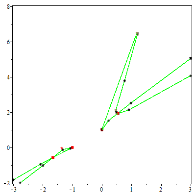
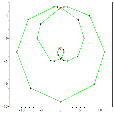
Figure 1: The left figure is the output of ptopo for the parametric curve $(\frac{3\,t^{2}+3\,t+1}{t^{6}-2\,t^{4}-3\,t-1},\frac{(t^{4}-2\,t+2)t^{2}}{t^{6}-2\,t^{4}-3\,t-1})$, while the right figure is the output for the curve $\small(\tfrac{6\,t^{8}-756\,t^{6}+3456\,t^{5}-31104\,t^{3}+61236\,{t}^{2}-39366}{t^{8}+36\,t^{6}+486\,t^{4}+2916\,t^{2}+6561}$, $\tfrac{-18(6\,t^{6}-16\,t^{5}-126\,t^{4}+864\,t^{3}-1134\,t^{2}-1296\,t+4374)t}{t^{8}+36\,t^{6}+486\,t^{4}+2916\,t^{2}+6561})$. Multiple points are indicated by red squares and isolated points by red stars.

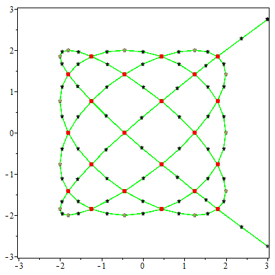
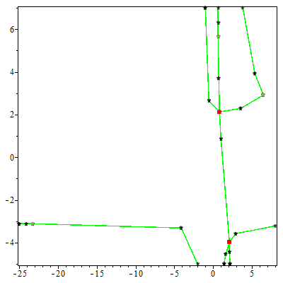
Figure 2: The left figure is the output of ptopo for the parametric curve $({t}^{8}-8\,{t}^{6}+20\,{t}^{4}-16\,{t}^{2}+2,{t}^{7}-7\,{t}^{5}+14\,{t}^{3}-7\,t)$ while the right figure is the output for the curve $(\frac{37\,{t}^{3}-23\,{t}^{2}+87\,t+44}{29\,{t}^{3}+98\,{t}^{2}-23\,t+10},\frac{-61\,{t}^{3}-8\,{t}^{2}-29\,t+95}{11\,{t}^{3}-49\,{t}^{2}-47\,t+40})$. Multiple points are indicated by red squares.

.

Theorem 24 (PTOPO and an abstract graph).

Consider a proper parametrization $\phi$ of curve $\mathcal{C}$ involving polynomials of degree $d$ and bitsize $\tau$, as in Eq. (1), that has no singularities at infinity. Alg. 3 outputs a graph $G$ that, if we embed it in $\mathbb{R}^{n}$, then it is isotopic to $\mathcal{C}$. It has worst case complexity

$$\widetilde{\mathcal{O}}_{B}(nd^{6}+nd^{5}\tau+d^{4}(n^{2}+n\tau)+d^{3}(n^{2}\tau+n^{3})+n^{3}d^{2}\tau),$$

while its expected complexity is

$$\widetilde{\mathcal{O}}_{B}(d^{6}+d^{5}(n+\tau)+d^{4}(n^{2}+n\tau)+d^{3}(n^{2}\tau+n^{3})+n^{3}d^{2}\tau),$$

If $n=\mathcal{O}(1)$, then bounds become $\widetilde{\mathcal{O}}_{B}(N^{6})$, where $N=\max\{d,\tau\}$.

Remark 25.

If we are given a box $\mathcal{B}\subset\mathbb{R}^{n}$ at the input, we slightly modify PTOPO, as follows: We discard the parameter values in $\mathtt{T}_{C}\cup\mathtt{T}_{M}\cup\mathtt{T}_{E}\cup\mathtt{T}_{I}$ that correspond to points not contained in $\mathcal{B}$. The set of $G$’s vertices is constructed similarly. To connect the vertices, we follow the same method with a minor modification: For any consecutive elements $t_{1}<t_{2}$ in a list $\mathtt{T}_{i}$ with more than two elements, such that $t_{1}\in\lambda(v_{i,1})$ and $t_{2}\in\lambda(v_{i,2})$, we add the edge $\{v_{i,1},v_{i,2}\}$ if and only if $\phi(t_{1})$, $\phi(t_{2})$ are not both on the boundary of $\mathcal{B}$; or in other words $t_{1}$ and $t_{2}$ are not both in $\mathtt{T}_{B}$.

6 Isotopic embedding for the special cases of plane and space curves

In this section we elaborate on the isotopic embedding of the output graph $G$ of Thm. 24 for the case of plane and space parametric curves $\mathcal{C}$. We embed every edge of the abstract graph $G$ in the corresponding parametric arc by sampling many parameter values in the associated parametric interval and then connecting the corresponding points accordingly, in $\mathbb{R}^{2}$ or $\mathbb{R}^{3}$. The larger the number of sampled parameters, the more likely it is for the embedding to be isotopic to $\mathcal{C}$. However, we might need a prohibitive large number of points to sample; their number is related to the distance between two branches of the curve. We show that by introducing a few additional points, we can replace the parametric arcs of the embedded graph with straight line segments and count on it being isotopic to $\mathcal{C}$. Following Alcázar et al. (2020) closely, if $X,Y\subset\mathbb{R}^{n}$ are one-dimensional, then being isotopic implies that one of them can be deformed into the other without removing or introducing self-intersections.

For plane curves, there is no need to take intermediate points on each parametric arc. We consider the embedding of the abstract graph $G$ in $\mathbb{R}^{2}$ as a straight-line graph $\tilde{G}$, i.e., with straight lines for edges, whose vertices are mapped to the corresponding points of the curve. The vertices of $\tilde{G}$ are all the singular and extreme points with respect to the $x$- and $y$- directions. Therefore, the edges of $\tilde{G}$ correspond to smooth and monotonous parametric arcs and so they cannot intersect but at their endpoints. The embedding $\tilde{G}$ is then trivially continuously deformed to $\mathcal{C}$. The above discussion summarizes as follows:

Corollary 26 (PTOPO and isotopic embedding for plane curves).

Consider a proper parametrization $\phi$ of a curve $\mathcal{C}$ in $\mathbb{R}^{2}$ involving polynomials of degree $d$ and bitsize $\tau$, as in Eq. (1), that has no singularities at infinity. Alg. 3 computes an abstract graph whose straight-line embedding in $\mathbb{R}^{2}$ is isotopic to $\mathcal{C}$ in worst case complexity $\widetilde{\mathcal{O}}_{B}(d^{6}+d^{5}\tau)$.

For space curves, a straight-line embedding of $G$ is not guaranteed to be isotopic to $\mathcal{C}$ for knots may be present. To overcome this issue, we need to segment some edges of $G$ into two or more edges. To find the extra vertices that we need to add to the graph, we follow a common approach (Alcázar and Díaz-Toca, 2010; Alcázar et al., 2020; Kahoui, 2008; Diatta et al., 2008; Cheng et al., 2013) that projects the space curve to a plane one. For a projection defined by the map $\pi:\mathcal{C}\rightarrow\mathbb{R}^{2}$, we write $\tilde{\mathcal{C}}=\pi(\mathcal{C})$. We will ensure in the sequel that the following two conditions are satisfied:

1. $\mathcal{C}$ has no asymptotes parallel to the direction of the projection.

2. The map $\pi$ is birational (Sendra et al., 2008, Def. 2.37).

The first condition is to ensure that the point at infinity $\mathbf{p}_{\infty}$ of $\mathcal{C}$ exists if and only if the point at infinity of $\tilde{\mathcal{C}}$ exists and is equal to $\pi(\mathbf{p}_{\infty})$ (Alcázar and Díaz-Toca, 2010, Lem. 10); see Fig.3(b) for an instance where this condition is violated. The second condition ensures that only a finite number of points on $\tilde{\mathcal{C}}$ have more than one point as a preimage. We call these points apparent singularities (Diatta et al., 2008); see Fig. 3(a). Thus, with this condition we avoid the ”bad” cases where two branches of $\mathcal{C}$ project to the same branch of $\tilde{\mathcal{C}}$.

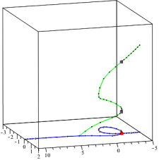
(a)

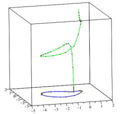
(b)

Figure 3: (a) Graph of the curve parametrized by $\phi(t)=\big{(}\frac{7t^{4}-22t^{3}+55t^{2}+94t-87}{56t^{4}+62t^{2}-97t+73},\frac{88t^{5}+4t^{4}-83t^{3}+10t^{2}-62t-82}{56t^{4}+62t^{2}-97t+73},-\frac{95t^{5}-4t^{4}+83t^{3}-10t^{2}+62t+82}{56t^{4}+73}\big{)}$ (green) and its orthogonal projection on the $xy$-plane (blue). In red, a double point in the projected curve with two points in its preimage, i.e., apparent singularities (purple). (b) Graph of the curve parametrized by $\phi(t)=\big{(}\frac{-7t^{4}+22t^{3}-55t^{2}-94t+87}{-56t^{4}-62t^{2}+97t-73},\frac{-4t^{4}+83t^{3}-10t^{2}+62t+82}{-56t^{4}-62t^{2}+97t-73},\frac{t^{7}-4t^{4}+83t^{3}-10t^{2}+62t+82}{-56t^{4}-73}\big{)}$ (green) and its orthogonal projection on the $xy$-plane (blue). The space curve does not have a point at infinity, whereas the plane curve has.

Lemma 27.

Consider a proper parametrization $\phi$ of curve $\mathcal{C}$ in $\mathbb{R}^{3}$ involving polynomials of degree $d$ and bitsize $\tau$, as in Eq. (1), that has no singularities at infinity. We compute a map $\pi:\mathcal{C}\rightarrow\mathbb{R}^{2}$ satisfying conditions (C1), (C2) in worst case complexity $\widetilde{\mathcal{O}}_{B}(d^{5}+d^{4}\tau)$ and using a Las Vegas algorithm in expected complexity $\widetilde{\mathcal{O}}_{B}(d^{3}+d^{2}\tau)$.

Proof.

By (Walker, 1978, Thm. 6.5, pg. 146), any space curve can be birationally projected to a plane curve. We choose an integer $a$ uniformly at random from the set $\{1,\dots Kd^{2}\}$, where $K=\mathcal{O}(1)$; we explain later in the proof about the size of this set. We define the mapping:

$$\pi:\quad \mathbb{C}^{3}\rightarrow\mathbb{C}^{2}$$

$$(x,y,z)\mapsto(x,y+az)$$ (5)

It will be useful in the sequel to regard the application of $\pi(\cdot)$ to $\phi(t)$ as being performed in two steps:

1. Change of orthogonal basis of $\mathbb{R}^{3}$: Let $\{\begin{pmatrix}1\\ 0\\ 0\end{pmatrix},\begin{pmatrix}0\\ 1\\ -a\end{pmatrix},\begin{pmatrix}0\\ a\\ 1\end{pmatrix}\}$ be an orthogonal basis of $\mathbb{R}^{3}$ and

   $$A=\begin{pmatrix}1&0&0\\ 0&1&a\\ 0&-a&1\\ \end{pmatrix}.$$

   In the new basis the curve is parametrized by:

   $$(\phi_{1}(t),\phi_{2}(t),\phi_{3}(t))\cdot A=(\phi_{1}(t),\phi_{2}(t)+a\phi_{3}(t),-a\phi_{2}(t)+\phi_{3}(t))$$

2. Orthogonal projection onto the first two coordinates: This yields the plane curve parametrized by $(\phi_{1}(t),\phi_{2}(t)+a\phi_{3}(t))$.

For a given choice of $a$, we check if conditions (C1) and (C2) are satisfied:

For (C1): The direction of the projection is defined by the vector $(0,a,1)$. So, $\mathcal{C}$ has no asymptotes parallel to $(0,a,1)$ if and only if the curve with parametrization $\phi(t)\cdot A$ has no asymptotes parallel to $(0,a,1)\cdot A^{-1}=(0,0,1)$. We can check if this is the case by employing (Alcázar and Díaz-Toca, 2010, Lem. 9); this is no more costly that solving a univariate polynomial of size $(\mathcal{O}(d),\widetilde{\mathcal{O}}(\tau))$, which costs $\widetilde{\mathcal{O}}_{B}(d^{3}+d^{2}\tau)$ worst case.

Morover, there are $\mathcal{O}(d)$ bad values of $a$ for whom (C1) does not hold: for any asymptote of $\mathcal{C}$, there is a unique value of $a$ that maps it to an asymptote parallel to $(0,0,1)$ in the new basis. The asymptotes of $\mathcal{C}$ are $\mathcal{O}(d)$ since they occur at the poles of $\phi(t)$ and at the branches that extend to infinity.

For (C2): Since $\phi(t)$ is proper, $\pi(\cdot)$ is birational if and only if $\pi(\phi(t))$ is also proper. We check the properness of this parametrization of $\tilde{\mathcal{C}}$ in $\widetilde{\mathcal{O}}_{B}(d^{3}+d^{2}\tau)$ expected time, using Lem. 5.

To find the values of $a$ that result in a ‘bad’ map: Let $\tilde{h_{1}}(s,t),\tilde{h_{2}}(s,t)$ be the polynomials of Eq. (1) associated to $\pi(\phi(t))$. The parametrization $\pi(\phi(t))$ is proper if and only if $\gcd(\tilde{h_{1}}(s,t),\tilde{h_{2}}(s,t))=1$. If $\gcd(\tilde{h_{1}}(s,t),\tilde{h_{2}}(s,t))\neq 1$ then, by letting $R(s)=\mathtt{res}_{t}(\tilde{h_{1}}(s,t),\tilde{h_{2}}(s,t))$, we have that $R(s)=0$. Notice that $R(s)$ is not always identically zero (e.g., for $\tilde{h_{1}}(s,t)=t+s,\tilde{h_{2}}(s,t)=t+s-1$ we get $R(s)=1$). We consider $R(s)$ as a polynomial in $\mathbb{Z}(a)[s]$:

$$R(s)=c_{d^{2}}(a)s^{d^{2}}+\dots+c_{1}(a)s+c_{0}(a),$$

where $c_{i}\in\mathbb{Z}[a]$ is of size $(d,\widetilde{\mathcal{O}}(d\tau))$ for $0\leq i\leq d^{2}$ . The bad values of $a\in\mathbb{R}$ satisfy then the equation:

$$c_{d^{2}}^{2}(a)+\dots+c_{1}^{2}(a)+c_{0}^{2}(a)=0.$$

The polynomial has degree $\mathcal{O}(d^{2})$ and so there are $\mathcal{O}(d^{2})$ bad values to avoid. This points to the worst case complexity $\widetilde{\mathcal{O}}_{B}(d^{5}+d^{4}\tau)$. ∎

Given a map $\pi$ computed through Lem. 27, we find the parameters that give the real multiple points of $\tilde{\mathcal{C}}$ and its extreme points with respect to the two coordinate axes. We add the corresponding vertices to $G$ and we obtain an augmented graph, say $G^{\prime}$. The straight-line embedding of $G^{\prime}$ in $\mathbb{R}^{2}$ is isotopic to $\tilde{\mathcal{C}}$ by Cor. 26, possibly up to the isolated points (Alcázar and Díaz-Toca, 2010, Thm. 13 and Lem. 15). Then, by lifting this embedding to the corresponding straight-line graph in $\mathbb{R}^{3}$, we obtain a graph isotopic to $\mathcal{C}$ (Alcázar and Díaz-Toca, 2010, Thm. 13 and Thm. 14). The following theorem summarizes the previous discussion and states its complexity:

Theorem 28 (PTOPO and isotopic embedding for 3D space curves).

Consider a proper parametrization $\phi$ of curve $\mathcal{C}$ in $\mathbb{R}^{3}$ involving polynomials of degree $d$ and bitsize $\tau$, as in Eq. (1), that has no singularities at infinity. There is an algorithm that computes an abstract graph whose straight-line embedding in $\mathbb{R}^{3}$ is isotopic to $\mathcal{C}$ in worst case complexity $\widetilde{\mathcal{O}}_{B}(d^{6}+d^{5}\tau)$.

Proof.

Given a projection map $\pi(\cdot)$ such that (C1) and (C2) hold, correctness follows from the previous discussion. From Lem. 27, we find such a map in expected complexity $\widetilde{\mathcal{O}}_{B}(d^{3}+d^{2}\tau)$ and $\widetilde{\mathcal{O}}_{B}(d^{5}+d^{4}\tau)$. Using Alg. 2 for $\pi(\phi(t))$ we find the parameters of the extreme (in the coordinate directions) and real multiple points of $\tilde{\mathcal{C}}$, say $\tilde{\mathtt{T}}$, in $\widetilde{\mathcal{O}}_{B}(d^{6}+d^{5}\tau)$ (Lem. 18). Then, we employ Alg. 3 for $\phi(t)$, by augmenting the list of parameters that are treated with $\tilde{\mathtt{T}}$. The last step dominates the complexity and is not affected by the addition of extra parameters to the list since $|\tilde{\mathtt{T}}|=\mathcal{O}(d^{2})$. The complexity result in Thm. 24 allows us to conclude. ∎

Remark 29.

The complexity in Thm. 28 is no higher than the complexity in Thm. 24, i.e., no costlier than the computation of the topology itself.

(a)

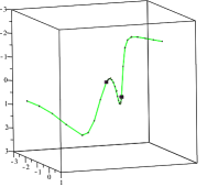
(b)

Figure 4: Output of PTOPO for (a) a Lissajous curve parametrized by $\big{(}\frac{(-t^{2}-1)}{t^{2}+1},\frac{-8t(t^{2}-1)(t^{4}-6t^{2}+1)}{t^{8}+4t^{6}+6t^{4}+4t^{2}+1},\frac{-(16(t^{4}-6t^{2}+1))(t^{2}-1)t(t^{8}-28t^{6}+70t^{4}-28t^{2}+1)}{(t^{1}6+8t^{1}4+28t^{1}2+56t^{1}0+70t^{8}+56t^{6}+28t^{4}+8t^{2}+1)}\big{)}$. The multiple points are indicated by the red squares. (b) a space curve parametrized by $\big{(}\frac{-2t^{2}}{t^{2}+1},\frac{-2t(3t^{5}-19t^{4}+8t^{3}-9t^{2}-t+2}{(t^{2}+1)(10t^{4}-6t^{3}+3t^{2}+1)},t\big{)}$. The apparent singularities are indicated by the black squares.

7 Multiplicities and characterization of singular points

We say that a singularity is ordinary if it is at the intersection of smooth branches only and the tangents to all branches are distinct (Walker, 1978, p.54). In all the other cases, we call it a non-ordinary singularity. The character of a singular point is either ordinary or non-ordinary. To determine the multiplicity and the character of each real singular point in $\mathbb{C}$ we follow the method presented in the series of papers Pérez-Díaz (2007); Blasco and Pérez-Díaz (2017, 2019). They provide a complete characterization using resultant computations that applies to curves of any dimension. In the sequel, we present the basic ingredients of their approach and we estimate the bit complexity of the algorithm.

Let $n=2$ and $H_{i}(s,t)=p_{i}(s)q_{i}(t)-p_{i}(t)q_{i}(s)$, for $i\in[2]$. Consider a point $\mathbf{p}\in\mathcal{C}$ given by the parameter values $\{s_{1},\dots,s_{k}\}$, $k\geq 1$; that is $\mathbf{p}=\phi(s_{i})$, for all $i\in[k]$. The fiber function at $\mathbf{p}$ (Blasco and Pérez-Díaz, 2019, Def. 2) is

$$F_{\mathbf{p}}(t)=\gcd(H_{1}(s_{j},t),H_{2}(s_{j},t)),$$

for any $j\in[k]$. It is a univariate polynomial, the real roots of which are the parameter values that correspond to the point $\mathbf{p}$. When the parametrization of the curve is proper, for any point $\mathbf{p}$ on $\mathcal{C}$ other than $\mathbf{p}_{\infty}$ it holds that $\deg(F_{\mathbf{p}}(t))=\text{mult}_{\mathbf{p}}(\mathcal{C})$ (Blasco and Pérez-Díaz, 2019, Cor. 1). Also, when the parameters in $\{s_{1},\dots,s_{k}\}$ are all real, $k$ equals the number of real branches that go through $\mathbf{p}$.

To classify ordinary and non-ordinary singularities we proceed as follows: For a point $\mathbf{p}\in\mathcal{C}$ the delta invariant $\delta_{\mathbf{p}}$ is a nonnegative integer that measures the number of double points concentrated around $\mathbf{p}$. We can compute it by taking into account the multiplicities of $\mathbf{p}$ and its neighboring singularities. Blasco and Pérez-Díaz (2019) consider three different types of non-ordinary singularities and use the delta invariant to distinguish them. In particular:

1. If $k=\text{mult}_{\mathbf{p}}(\mathcal{C})$ and $2\delta_{\mathbf{p}}=\text{mult}_{\mathbf{p}}(\mathcal{C})(\text{mult}_{\mathbf{p}}(\mathcal{C})-1)$, then $\mathbf{p}$ is an ordinary singularity.

2. If $k<\text{mult}_{\mathbf{p}}(\mathcal{C})$ and $2\delta_{\mathbf{p}}=\text{mult}_{\mathbf{p}}(\mathcal{C})(\text{mult}_{\mathbf{p}}(\mathcal{C})-1)$, then $\mathbf{p}$ is a type $I$ non-ordinary singularity.

3. If $k=\text{mult}_{\mathbf{p}}(\mathcal{C})$ and $2\delta_{\mathbf{p}}>\text{mult}_{\mathbf{p}}(\mathcal{C})(\text{mult}_{\mathbf{p}}(\mathcal{C})-1)$, then $\mathbf{p}$ is a type $II$ non-ordinary singularity.

4. If $k<\text{mult}_{\mathbf{p}}(\mathcal{C})$ and $2\delta_{\mathbf{p}}>\text{mult}_{\mathbf{p}}(\mathcal{C})(\text{mult}_{\mathbf{p}}(\mathcal{C})-1)$, then $\mathbf{p}$ is a type $III$ non-ordinary singularity.

Blasco and Pérez-Díaz (2019) compute the delta invariant, $\delta_{\mathbf{p}}$, using the formula

$$\delta_{\mathbf{p}}=\frac{1}{2}\sum_{j=1}^{k}\sum_{t\text{ s.t. }h_{1}(s_{j},t)=h_{2}(s_{j},t)=0}\text{Int}_{h_{1},h_{2}}(s_{j},t),$$ (6)

where $\text{Int}_{h_{1},h_{2}}(\alpha,\beta)$ is the intersection multiplicity of the coprime polynomials $h_{1}(s,t)$ and $h_{2}(s,t)$ at a point $(\alpha,\beta)$. Using a well known result, e.g., (Fulton, 1984, 1.6) as stated in (Busé et al., 2005, Prop. 5), we can compute the intersection multiplicities using resultant computations. Let $R(s)=\mathtt{res}_{t}(h_{1}(s,t),h_{2}(s,t))$. For a root $\alpha$ of $R(s)$, its multiplicity $\mu(a)$ is equal to the sum of the intersection multiplicities of solutions of the system of $\{h_{1},h_{2}\}$ in the form $(\alpha,t)$, and so

$$\mu(\alpha)=\sum_{t\text{ s.t. }h_{1}(\alpha,t)=h_{2}(\alpha,t)=0}\text{Int}_{h_{1},h_{2}}(\alpha,t).$$ (7)

Therefore, from Eq. (6) and Eq. (7), we conclude that:

$$\delta_{\mathbf{p}}=\frac{1}{2}\sum_{j=1}^{k}\mu(s_{j}).$$ (8)

For space curves, we birationally project $\mathcal{C}$ to a plane curve (Walker, 1978, Thm. 6.5, pg. 146). The multiplicities of the singular points of $\mathcal{C}$ and their delta invariant are preserved under the birational map realizing the projection (Blasco and Pérez-Díaz, 2019, Prop. 1 and Cor. 4). The pseudo code of the algorithm appears in Alg. 4.

Input: Proper parametrization $\phi\in\mathbb{Z}(t)^{n}$ without singularity at infinity, as in Eq. (1)

1

Output: Multiplicities and characterization of points

2

3$\mathcal{S}\leftarrow$ Special_Points($\phi$)

4if n=2 then

5       Compute polynomials $H_{1}(s,t),H_{2}(s,t)$ for $\phi$

6else

7       repeat

8             Choose integers $a_{3},\dots,a_{n}$ at random from $\{1,\dots,Kd^{n}\}$, where $K=\mathcal{O}(1)$.

9            $\tilde{\phi}(t)\leftarrow(\phi_{1}(t),\phi_{2}(t)+a_{3}\phi_{3}(t)+\dots+a_{n}\phi_{n}(t))$

10      until $\tilde{\phi}(t)$ is proper;

11      Compute polynomials $H_{1}(s,t),H_{2}(s,t)$ for $\tilde{\phi}$

12

13for $\mathbf{p}\in\mathcal{S}$ do

14      

      $M_{\mathbf{p}}\leftarrow\left\{s\in\mathbb{R}:\phi(s)=\mathbf{p}\right\}$ // parameters that give the same point $\mathbf{p}$

15      

      $k\leftarrow|M_{\mathbf{p}}|$ // number of real branches that go through $\mathbf{p}$

16      

17      Take $s_{0}\in M_{\mathbf{p}}$

      $\text{mult}_{\mathbf{p}}(\mathcal{C})\leftarrow\deg(\gcd(H_{1}(s_{0},t),H_{2}(s_{0},t)))$ // multiplicity

18      

      // compute delta invariant

19      

20      $\delta_{\mathbf{p}}\leftarrow 0$

21      for $s_{j}\in M_{\mathbf{p}}$ do

22            

23            $\mu(s_{j})\leftarrow$ multiplicity of $s_{j}$ as a root of $\mathtt{res}_{t}(H_{1}(s,t)/(s-t),H_{2}(s,t)/(s-t))$

24            $\delta_{\mathbf{p}}\leftarrow\delta_{\mathbf{p}}+\mu(s_{j})$

25      $\delta_{\mathbf{p}}\leftarrow\delta_{\mathbf{p}}/2$

26      if $k=\text{mult}_{\mathbf{p}}(\mathcal{C})$ and $2\delta_{\mathbf{p}}=\text{mult}_{\mathbf{p}}(\mathcal{C})(\text{mult}_{\mathbf{p}}(\mathcal{C})-1)$  then

27             return $\mathbf{p}$ is an ordinary singularity

28      else if $k<\text{mult}_{\mathbf{p}}(\mathcal{C})$ and $2\delta_{\mathbf{p}}=\text{mult}_{\mathbf{p}}(\mathcal{C})(\text{mult}_{\mathbf{p}}(\mathcal{C})-1)$ then

29             return $\mathbf{p}$ is a type $I$ non-ordinary singularity

30      else if $k=\text{mult}_{\mathbf{p}}(\mathcal{C})$ and $2\delta_{\mathbf{p}}>\text{mult}_{\mathbf{p}}(\mathcal{C})(\text{mult}_{\mathbf{p}}(\mathcal{C})-1)$ then

31             return $\mathbf{p}$ is a type $II$ non-ordinary singularity

32      else if $k<\text{mult}_{\mathbf{p}}(\mathcal{C})$ and $2\delta_{\mathbf{p}}>\text{mult}_{\mathbf{p}}(\mathcal{C})(\text{mult}_{\mathbf{p}}(\mathcal{C})-1)$ then

33             return $\mathbf{p}$ is a type $III$ non-ordinary singularity

34      

35

Algorithm 4 CharacterizeSingularPoints($\phi,\mathcal{S}$)

Theorem 30.

Let $\mathcal{C}$ be a curve with a proper parametrization $\phi(t)$ as in Eq. (1), that has no singularities at infinity. Alg. 4 computes the singular points of $\mathcal{C}$, their multiplicity and character (ordinary/non-ordinary) in

$$\widetilde{\mathcal{O}}_{B}(d^{6}+d^{5}\tau)$$

worst-case complexity when $n=2$ and for $n>2$ in expected complexity

$$\widetilde{\mathcal{O}}_{B}(d^{6}+d^{5}(n+\tau)+d^{4}(n^{2}+n\tau)+d^{3}(n^{2}\tau+n^{3})+n^{3}d^{2}\tau).$$

Proof.

We compute the parameters that give the singular points of $\mathcal{C}$ using Alg. 2 in $\widetilde{\mathcal{O}}_{B}(d^{6}+d^{5}(n+\tau)+d^{4}(n^{2}+n\tau)+d^{3}(n^{2}\tau+n^{3})+n^{3}d^{2}\tau)$ when $n>2$, which becomes worst-case when $n=2$ (Lem. 18).

When $n>2$, lines 5-8 compute a birational projection of $\mathcal{C}$ to a plane curve parametrized by $\tilde{\phi}(t)$ (note that the projection is birational if and only if $\tilde{\phi}(t)$ is proper since $\phi(t)$ is proper). The expected complexity of this is $\widetilde{\mathcal{O}}_{B}(d^{3}+nd^{2}\tau)$ by slightly adapting the proof of Lem. 27.

We can group the parameter values that give singular points using Lem. 22 in $\mathcal{O}(d^{2}+nd)$ arithmetic operations. We have that $\gcd(H_{1}(s,t),H_{2}(s,t))=s-t$. For $h_{1}(s,t)=H_{1}(s,t)/(s-t)$, $h_{2}(s,t)=H_{2}(s,t)/(s-t)$, we compute a triangular decomposition of the system $\{h_{1}(s,t)=h_{2}(s,t)=0\}$ which consists of the systems $\{(A_{i}(s),B_{i}(s,t))\}_{i\in\mathcal{I}}$. For any root $\alpha$ of $A_{i}$, $B_{i}(\alpha,t)$ is of degree $i$ and equals $\gcd(h_{1}(\alpha,t),h_{2}(\alpha,t))$ (up to a constant factor). By (Bouzidi et al., 2015a, Prop. 16), the triangular decomposition is computed in $\widetilde{\mathcal{O}}_{B}(d^{6}+d^{5}\tau)$ worst case.

For a singular point $\mathbf{p}$ and $s_{0}\in M_{\mathbf{p}}$: To compute the degree of $\gcd(H_{1}(s_{0}),H_{2}(s_{0}))$, since $s_{0}$ is a root of $\mathtt{res}_{t}(h_{1}(s,t),h_{2}(s,t))$, it suffices to find for which $i\in\mathcal{I}$ $A_{i}(s_{0})=0$. The latter is not immediate when $s_{0}$ is given in isolated interval representation as a root of $\mathtt{res}_{t}(h_{1}(s,t),h_{2}(s,t))$. However, we can isolate the roots of all $A_{i}$ by taking care that the isolating invervals are small enough so that the isolating interval of $s_{0}$ intersects only one of them. Because they are roots of the same polynomial this cannot exceed the complexity of isolating the roots of $\mathtt{res}_{t}(h_{1}(s,t),h_{2}(s,t))$. This is can be done in $\widetilde{\mathcal{O}}_{B}(d^{6}+d^{5}\tau)$. In the same bit complexity, we have the multiplicity $\mu(s_{j})$ of $s_{j}$ as a root of $\mathtt{res}_{t}(h_{1},h_{2})$. ∎

8 Implementation and examples

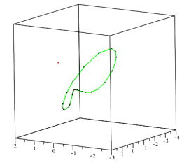
(a)

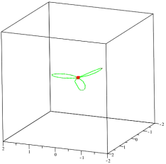
(b)

Figure 5: Output of PTOPO for a curve parametrized by (a) $\big{(}\frac{-7t^{4}+22t^{3}-55t^{2}-94t+87}{-56t^{4}-62t^{2}+97t-73},\frac{-4t^{4}*83t^{3}-10t^{2}-62t-82}{-56t^{4}-62t^{2}+97t-73},\frac{-4t^{4}*83t^{3}-10t^{2}-62t-82}{-56t^{4}-62t^{2}+97t-73}\big{)}$ (b) $\big{(}\frac{-3t^{2}+1}{(t^{2}+1)^{2}},\frac{(-3t^{2}+1)t}{(t^{2}+1)^{2}},\frac{(-3t^{2}+1)t^{3}}{(t^{2}+1)^{4}\big{)}}$. The red star in (a) corresponds to an isolated point, whereas the red square in (b) corresponds to a multiple point. Examples are taken from Alcázar and Díaz-Toca (2010).

PTOPO is implemented in maple for plane and 3D curves. A typical output appears in Figures 1, 2, 5(a), and 5(b). Besides the visualization the software computes all the points of interest of curve (singular, extreme, etc) in isolating interval representation as well as in suitable floating point approximations.

We build upon the real root isolation routines of maple’s RootFinding library and the slv package (Diochnos et al., 2009), to use a certified implementation of general purpose exact computations with one and two real algebraic numbers, like comparison and sign evaluations, as well as exact (bivariate) polynomial solving.

PTOPO computes the topology and visualizes parametric curves in two (and in the near future in three) dimensions. For a given parametric representation of a curve, PTOPO computes the special points on the curve, the characteristic box, the corresponding graph, and then it visualizes the curve (inside the box). The computation, in all examples from literature we tested, takes less than a second in a MacBook laptop, running maple 2020. We refer the reader to the website of the software and to (Katsamaki et al., 2020b) for further details.

Acknowledgments

We acknowledge partial support by the Fondation Mathématique Jacques Hadamard through the PGMO grand ALMA, by ANR JCJC GALOP (ANR-17-CE40-0009), by the PHC GRAPE, by the projects 118F321 under the program 2509, 118C240 under the program 2232, and 117F100 under the program 3501 of the Scientific and Technological Research Council of Turkey.

References

-
Abhyankar and Bajaj (1989)
Abhyankar, S. S., Bajaj, C. J., 1989. Automatic parameterization of rational
curves and surfaces IV: Algebraic space curves. ACM Trans. Graph. 8 (4),
325–334.
URL https://doi.org/10.1145/77269.77273 -
Alberti et al. (2008)
Alberti, L., Mourrain, B., Wintz, J., 2008. Topology and arrangement
computation of semi-algebraic planar curves. CAGD 25 (8), 631 – 651.
URL http://www.sciencedirect.com/science/article/pii/S0167839608000460 -
Alcázar et al. (2020)
Alcázar, J. G., Caravantes, J., Díaz, G. M., Tsigaridas, E., 2020.
Computing the topology of a plane or space hyperelliptic curve. Computer
Aided Geometric Design 78, 101830.
URL http://www.sciencedirect.com/science/article/pii/S0167839620300170 -
Alcázar and Díaz-Toca (2010)
Alcázar, J. G., Díaz-Toca, G. M., 2010. Topology of 2D and 3D rational
curves. CAGD 27 (7), 483 – 502.
URL http://www.sciencedirect.com/science/article/pii/S0167839610000737 - Basu et al. (2003) Basu, S., Pollack, R., M-F.Roy, 2003. Algorithms in Real Algebraic Geometry. Vol. 10 of Algorithms and Computation in Mathematics. Springer-Verlag.
- Bernardi et al. (2016) Bernardi, A., Gimigliano, A., Idà, M., 09 2016. Singularities of plane rational curves via projections. J. Symb. Comput.
-