Optimal networks for dynamical spreading

Liming Pan School of Computer and Electronic Information, Nanjing Normal University, Nanjing, Jiangsu, 210023, China    Wei Wang wwzqbx@hotmail.com Cybersecurity Research Institute, Sichuan University, Chengdu 610065, China    Lixin Tian School of Mathematical Sciences, Nanjing Normal University, Nanjing, Jiangsu 210023, China    Ying-Cheng Lai School of Electrical, Computer and Energy Engineering, Arizona State University, Tempe, Arizona 85287, USA Department of Physics, Arizona State University, Tempe, Arizona 85287, USA
Abstract

The inverse problem of finding the optimal network structure for a specific type of dynamical process stands out as one of the most challenging problems in network science. Focusing on the susceptible-infected-susceptible type of dynamics on annealed networks whose structures are fully characterized by the degree distribution, we develop an analytic framework to solve the inverse problem. We find that, for relatively low or high infection rates, the optimal degree distribution is unique, which consists of no more than two distinct nodal degrees. For intermediate infection rates, the optimal degree distribution is multitudinous and can have a broader support. We also find that, in general, the heterogeneity of the optimal networks decreases with the infection rate. A surprising phenomenon is the existence of a specific value of the infection rate for which any degree distribution would be optimal in generating maximum spreading prevalence. The analytic framework and the findings provide insights into the interplay between network structure and dynamical processes with practical implications.

I Introduction

In the study of dynamics on complex networks, most previous efforts were focused on the forward problem: How does the network structure affect the dynamical processes on the network? The approaches undertaken to address this question have been standard and relatively straightforward: One implements the dynamical process of interest on a given network structure and then studies how alterations in the network structure affect the dynamics. The dynamical inverse problem is much harder: finding a global network structure that optimizes a given type of dynamical processes. Despite the extensive and intensive efforts in the past that have resulted in an essential understanding of the interplay between dynamical processes and network structure, previous studies of the inverse problem were sporadic and limited to a perturbation type of analysis, generating solutions that are at most locally optimal only Aguirre et al. (2013); Pan et al. (2019). The purpose of this paper is to present and demonstrate an analytic framework to address the dynamical inverse problem.

To be concrete, we will focus on spreading dynamics on networks for which a large body of literature has been generated in the past on the forward problem, i.e., how network topology affects the characteristics of the spreading, such as the outbreak threshold and prevalence Pastor-Satorras et al. (2015); Castellano et al. (2009). For example, under the annealed assumption that all nodes with the same degree are statistically equivalent, it was found Pastor-Satorras and Vespignani (2001) that the epidemic threshold of the susceptible-infected-susceptible (SIS) process is given by $\langle k\rangle/\langle k^{2}\rangle$, where $\langle k\rangle$ and $\langle k^{2}\rangle$ are the first and second moments of the degree distribution, respectively. In situations where the second moment diverges, the threshold value is essentially zero, meaning that the presence of a few hub nodes can greatly facilitate the occurrence of an epidemic outbreak. An understanding of the interplay between the network structure and the spreading dynamics is essential to articulating control strategies. For example, the important role played by the hub nodes suggests a mitigation strategy: Vaccinating these nodes can block or even stop the spread of the disease Cohen et al. (2003); Pastor-Satorras and Vespignani (2002). Likewise, if the goal is to promote information spreading, then choosing the hub nodes as the initial seeds can be effective Kitsak et al. (2010); Lü et al. (2016).

The inverse problem is motivated by the application scenarios in which one strives to optimize the network structure to achieve desired or improved performance Valente (2012). Optimization and invention have been applied to problems such as virus marketing Goel et al. (2016), social robots detection Ferrara et al. (2016), containment of false news spreading Vosoughi et al. (2018), and polarization reduction in social networks Musco et al. (2018). For spreading dynamics on networks, the few existing studies are focused on applying small perturbations to the network structure to modulate the dynamical process Aguirre et al. (2013); Pan et al. (2019). From the point of view of optimization, since the perturbations are local, the resulting solution is locally optimal at best.

We address the following questions: Does a globally optimal network exist and if yes, can it be found to maximize the prevalence of the spreading dynamics? Such a network is necessarily extremum. For general types of spreading dynamics, to analytically solve this inverse problem is currently not feasible. However, we find that the SIS type of spreading dynamics does permit an analytic solution. In particular, the annealed approximation stipulates that the network structure can be fully captured or characterized by its degree distribution. The problem of finding the optimal networks can then be formulated as one to find the optimal degree distribution that maximizes the prevalence of the SIS spreading dynamics, which can be analytically solved by exploiting the heterogeneous mean-field (HMF) theory Pastor-Satorras et al. (2015). Notwithstanding the necessity of imposing the annealed approximation to enable analytic solutions, the essential physical ingredients of the SIS dynamics are retained.

Our main results are the following. Taking a variational approach to solving the HMF equation, we obtain a necessary condition for the optimal degree distribution. The condition defines a set of candidate optimal degree distributions, and we show that a degree distribution is globally optimal if and only if it belongs to the set. However, if the set is empty, which can occur for relatively low and high infection rates, the necessary condition stipulates that a local extremum distribution must concentrate on no more than two distinct nodal degree values thereby substantially narrowing the search for the optimal network. Searching through all possible distributions under the constraint leads to the optimal degree distribution that can be proved to be unique. For intermediate infection rates, multiple optimal degree distributions with a broader support exist, which lead to identical spreading prevalence. In addition, our theory predicts the existence of a particular value of the infection rate for which every degree distribution is optimal. A general trend is that the degree heterogeneity of the optimal distribution decreases with the infection rate.

Our paper represents a first step toward finding a global optimal network structure for spreading dynamics. From a theoretical point of view, developing a method to find such extremum networks represents a feat that would provide deeper insights into the interplay between network topology and spreading dynamics. From a practical perspective, the solution can be exploited to design networks that are capable of spreading information or transporting material substances in the most efficient way possible.

In Sec. II, we introduce the HMF theory for the SIS dynamics and set up the basic framework for the optimization problem. In Sec. III, we employ a variational method to derive the necessary condition for a degree distribution to be an extremum among all feasible distributions. Solutions of the optimal degree distribution are presented in Sec. IV, and its properties are discussed in Sec. V. The paper is concluded in Sec. VI with a discussion.

II Problem formulation and sketch of major mathematical steps

In the SIS model, each node can be either in the susceptible or in the infected state, and we assume the nodal state evolves continuously with time. During the spreading process, a susceptible node is infected by its neighbors with the rate $\lambda$, whereas an infected node recovers at the rate $\gamma$. To study the equilibrium properties of the dynamical process, it is convenient to set $\gamma=1$ so that $\lambda$ is the sole dynamical parameter.

In the HMF theory, all the nodes with the same degree are statistically equivalent Pastor-Satorras et al. (2015). Consider a vector of nodal degrees $\mathbf{k}\equiv[k_{1},k_{2},\cdots,k_{n}]^{T}$, where the elements are arranged in a descending order: $k_{1}>k_{2}>\cdots>k_{n}$. The degree distribution is fully specified by a probability vector defined as $\mathbf{p}\equiv[p_{1},p_{2},\cdots,p_{n}]^{T}$, where $p_{i}\geq 0$ is the probability that a randomly chosen node has degree $k_{i}$. Let $x_{i}(t)$ be the probability that a node with degree $k_{i}$ is infected at time $t$. Given the probability vector $\mathbf{p}$, the HMF equation is

$$\frac{dx_{i}(t)}{dt}=-x_{i}(t)+\lambda k_{i}\left[1-x_{i}(t)\right]\Theta$$ (1)

for $i\in\{1,\cdots,n\}$, where

$$\Theta=\frac{1}{\langle k\rangle}\sum_{j=1}^{n}p_{j}k_{j}x_{j}(t).$$ (2)

In Ref. Wang and Dai (2008), it was proved that the HMF equation has a unique global stable equilibrium point $x^{*}$. In addition, for $\lambda<\langle k\rangle/\langle k^{2}\rangle$, we have $x^{*}_{i}=0$ for all $i\in\{1,\cdots,n\}$, whereas for $\lambda>\langle k\rangle/\langle k^{2}\rangle$, we have $0<x^{*}_{i}<1$ for all $i\in\{1,\cdots,n\}$. The spreading prevalence in the equilibrium state is

$$\psi(\mathbf{p})=\sum_{i=1}^{n}p_{i}x_{i}^{*},$$ (3)

where, to simplify the notations, we have omitted the dependence of $\psi(\mathbf{p})$ on $\lambda$. Let $\mathcal{P}$ be the family of all degree distributions with a fixed average degree defined on $\mathbf{k}$. That is, with a prespecified constant $z>0$, for any $\mathbf{p}\in\mathcal{P}$, we have $\sum_{i=1}^{n}p_{i}k_{i}=z$. Our goal is to find $\mathbf{p}^{o}\in\mathcal{P}$ that maximizes $\psi(\mathbf{p})$:

$$\mathbf{p}^{o}=\underset{\mathbf{p}\in\mathcal{P}}{\mathrm{argmin}}\ \psi(\mathbf{p}).$$ (4)

The optimization problem is nontrivial only when the value of $\lambda$ is larger than the epidemic threshold at least for one $\mathbf{p}\in\mathcal{P}$. The Bhatia-Davis inequality stipulates that the second moment of $\mathbf{p}$ is maximized when $\mathbf{p}$ concentrates on the end points $k_{1}$ and $k_{n}$. In this case, the second moment is $\langle k^{2}\rangle=zk_{1}+zk_{n}-k_{1}k_{n}$. The optimization problem is nontrivial only when the following condition is met:

$$\lambda>\lambda_{1}\equiv\frac{z}{zk_{1}+zk_{n}-k_{1}k_{n}}.$$ (5)

In this case, if there is a unique solution $\mathbf{p}$ such that $\lambda>z/\langle k^{2}\rangle$, it gives the optimal degree distribution $\mathbf{p}^{o}$.

Our goal is to analytically find the solutions for the optimization problem defined in Eq. (4). As the mathematical derivations involved are lengthy, it may be useful to sketch the basic idea, tools used, and the results, which we organize as the following three major steps.

  1. 1.

    Mathematically, Eq. (4) defines a variational problem for the HMF equations in Eq. (1), which can be studied through the standard calculus-of-variation techniques. In Sec. III.1, we adopt a variational approach for the HMF equations in Eq. (1) and derive the necessary condition for a degree distribution to be optimal. In particular, we impose a perturbation to the degree distribution as $\mathbf{p}^{\prime}=\mathbf{p}+\alpha\bar{\mathbf{p}}$ and derive a formula that predicts $\bar{\psi}(\mathbf{p},\mathbf{p}^{\prime})$, the part of the incremental spreading prevalence which is linear in $\alpha$. For $\mathbf{p}$ to be a candidate maximum, $\bar{\psi}(\mathbf{p},\mathbf{p}^{\prime})$ must be nonpositive for any choice of $\bar{\mathbf{p}}$, and this leads to the necessary condition for the local minima.

  2. 2.

    The next task is to study the necessary condition resulting from the variational analysis. In Sec. III.2, through a sequence of algebraic arguments, we show that for any $\mathbf{p}$ satisfying the necessary condition, it is only possible to have either (i) $\bar{\psi}(\mathbf{p},\mathbf{p}^{\prime})=0$ or (ii) $\bar{\psi}(\mathbf{p},\mathbf{p}^{\prime})<0$ for all feasible perturbations. This means that it is impossible to find a certain $\mathbf{p}$ such that $\bar{\psi}(\mathbf{p},\mathbf{p}^{\prime})=0$ and $\bar{\psi}(\mathbf{p},\mathbf{p}^{\prime\prime})<0$ for $\mathbf{p}^{\prime}\neq\mathbf{p}^{\prime\prime}$. Further, in Sec. III.2, we show that the condition $\bar{\psi}(\mathbf{p},\mathbf{p}^{\prime})=0$ can be reduced to a linear equation in $\mathbf{p}$ [the first equation in (25)] which, together with the probability constraint $\sum_{i=1}^{n}p_{i}=1$ and the average degree constraint $\sum_{i=1}^{n}p_{i}k_{i}=z$, defines a set of candidate optimal degree distributions $\mathcal{P}^{o}$. In Sec. III.3, by analyzing the three linear equations, we show that if $\mathcal{P}^{o}$ is nonempty, then any $\mathbf{p}$ is a global maximum if and only if $\mathbf{p}\in\mathcal{P}^{o}$. Concurrently, if $\mathcal{P}^{o}$ is empty, the optimal degree distribution with $\bar{\psi}(\mathbf{p},\mathbf{p}^{\prime})<0$ will concentrate on no more than two distinct nodal degrees.

  3. 3.

    Finally, in Sec. IV.1, we derive the condition when the set $\mathcal{P}^{o}$ is nonempty by analyzing the three linear equations defining the set [Eq. (25)]. In particular, $\mathcal{P}^{o}$ is nonempty for $\lambda\in[\lambda_{2},\ \lambda_{3}]$ (see Sec. IV.1 for explicit definitions of $\lambda_{2}$ and $\lambda_{3}$). For $\lambda<\lambda_{2}$ or $\lambda>\lambda_{3}$ and $\mathcal{P}^{o}$ indeed empty, we find the optimal degree distributions by solving the HMF equations explicitly (Sec. IV.2).

III Necessary condition for local extrema and consequences

In this section, we first study the optimization problem defined in Eq. (4) using several techniques from the calculus of variation. The calculation provides a necessary condition for finding the local maxima. We then analyze the necessary condition in detail to find the global optimal degree distributions.

III.1 Variational method

We study the variation problem in Eq. (4) using the standard techniques from the calculus of variations. Briefly, we apply a perturbation to the degree distribution $\mathbf{p}$ in Eq. (1) and calculate the linear response for the spreading prevalence. A local maximum necessarily has non-positive linear responses for any feasible perturbation.

For a fixed $\lambda>\langle k\rangle/\langle k^{2}\rangle$, let $x^{*}$ be the corresponding globally stable equilibrium point of the HMF equation. We impose a small variation on $p_{i}$,

$$p^{\prime}_{i}=p_{i}+\alpha\bar{p}_{i},$$ (6)

where $\bar{\mathbf{p}}$ specifies the direction of the variation and $\alpha>0$ controls its magnitude. For the perturbed degree distribution to be feasible, i.e., $\mathbf{p}^{\prime}\in\mathcal{P}$, the following conditions are necessary:

$$\sum_{i=1}^{n}\bar{p}_{i}=0\ \ \hbox{and}\ \ \sum_{i=1}^{n}\bar{p}_{i}k_{i}=0.$$ (7)

In addition, the perturbed degree distribution $\mathbf{p}^{\prime}$ must satisfy the probability constraints $0\leq p^{\prime}_{i}\leq 1$.

Let $x^{\prime}(t,\alpha)$ be the trajectory of the perturbed system. The time evolution of $x^{\prime}(t,\alpha)$ is described by the HMF equation with $\mathbf{p}$ replaced by $\mathbf{p}^{\prime}$ and $x_{i}(t)$ in Eq. (1) by $x_{i}^{\prime}(t,\alpha)$. As shown in Appendix A, $\mathbf{x}^{*}$ is a continuously differentiable function of $\mathbf{p}$ for $\lambda>z/\langle k^{2}\rangle$, enabling the following expansion of $x^{\prime}(t,\alpha)$ about $x^{*}_{i}$:

$$x^{\prime}_{i}(t,\alpha)=x^{*}_{i}+\alpha\bar{x}_{i}(t)+o(\alpha),$$ (8)

where $\bar{x}_{i}(t)$ is the response to the perturbation which is linear in $\alpha$. Taking the derivative with respect to $\alpha$ at $\alpha=0$, we obtain $\partial x^{\prime}_{i}(t,\alpha)/\partial\alpha|_{\alpha=0}=\bar{x}_{i}(t)$. The time derivative of $\bar{x}_{i}(t)$ is then given by

$$\begin{split}\frac{d\bar{x}_{i}(t)}{dt}&=\frac{\partial}{\partial\alpha}\bigg{|}_{\alpha=0}\frac{dx_{i}(t,\alpha)}{dt},\end{split}$$ (9)

which, after some algebraic manipulations, can be rewritten as

$$\frac{d\bar{\mathbf{x}}(t)}{dt}=\mathcal{J}\bar{\mathbf{x}}(t)+\xi,$$ (10)

where $\mathcal{J}$ is the $n\times n$ Jacobian matrix that does not depend on $\bar{\mathbf{p}}$ and $\xi$ is a vector of length $n$ that depends on $\bar{\mathbf{p}}$. The elements of $\mathcal{J}$ and $\xi$ are given by

$$J_{ij}=-\delta_{i,j}\left(1+\lambda k_{i}\Theta^{*}\right)+\frac{\lambda}{z}k_{i}\left(1-x^{*}_{i}\right)k_{j}p_{j},$$ (11)

and

$$\xi_{i}=\frac{\lambda}{z}k_{i}\left(1-x^{*}_{i}\right)\sum_{j=1}^{n}k_{j}\bar{p}_{j}x^{*}_{j},$$ (12)

respectively. In Eq. (11), $\delta_{i,j}$ is the Kronecker $\delta$ and $\Theta^{*}$ is obtained by substituting $\mathbf{x}(t)=\mathbf{x}^{*}$ into Eq. (2).

Equation (10) defines a linear system with the solution,

$$\bar{\mathbf{x}}(t)=\mathrm{e}^{\mathcal{J}t}\bar{\mathbf{x}}(0)+\left(\mathrm{e}^{\mathcal{J}t}-\mathcal{I}\right)\mathcal{J}^{-1}\xi,$$ (13)

where $\mathrm{e}^{\mathcal{J}t}$ is the matrix exponential of $\mathcal{J}t$. In Appendix B, we show that the eigenvalues of $\mathcal{J}$ have negative real parts. In the long time limit, we then have

$$\bar{\mathbf{x}}^{*}=\lim_{t\to\infty}\bar{\mathbf{x}}(t)=-\mathcal{J}^{-1}\xi.$$ (14)

With the perturbed degree distribution and Eq. (8), we can express the spreading prevalence as

$$\psi(\mathbf{p}^{\prime})=\psi(\mathbf{p})+\alpha\bar{\psi}\left(\mathbf{p},\mathbf{p}^{\prime}\right)+o(\alpha),$$ (15)

where $\bar{\psi}(\mathbf{p},\mathbf{p}^{\prime})$ is the part of incremental spreading prevalence that is linear in $\alpha$,

$$\bar{\psi}(\mathbf{p},\mathbf{p}^{\prime})=\sum_{i=1}^{n}\left(\bar{p}_{i}x^{*}_{i}+p_{i}\bar{x}^{*}_{i}\right).$$ (16)

Substituting Eq. (14) into Eq. (16), we have (after some algebraic manipulations)

$$\bar{\psi}(\mathbf{p},\mathbf{p}^{\prime})=\sum_{i=1}^{n}\chi_{i}\bar{p}_{i},$$ (17)

where $\chi_{i}$ is given by

$$\chi_{i}=x^{*}_{i}\left(1+\frac{\lambda k_{i}\Theta^{*}\sum_{j=1}^{n}p_{j}k_{j}(1-x^{*}_{j})^{2}}{\sum_{j=1}^{n}p_{j}k_{j}(x^{*}_{j})^{2}}\right),$$ (18)

The detailed derivation of Eq. (18) is presented in Appendix C. The necessary condition for the degree distribution $\mathbf{p}$ to be a local maximum is if and only if the inequality $\bar{\psi}(\mathbf{p},\mathbf{p}^{\prime})\leq 0$ holds for all feasible perturbations.

III.2 Consequences of the necessary condition

Equations (17) and (18) allow us to significantly narrow the search range for the optimal degree distribution through the process of elimination. In the following, we analyze the necessary condition by proving that it is only possible to have either (i) $\bar{\psi}(\mathbf{p},\mathbf{p}^{\prime})=0$ or (ii) $\bar{\psi}(\mathbf{p},\mathbf{p}^{\prime})<0$ for all feasible perturbations. That is, it is impossible to find $\mathbf{p}$ such that $\bar{\psi}(\mathbf{p},\mathbf{p}^{\prime})=0$ and $\bar{\psi}(\mathbf{p},\mathbf{p}^{\prime\prime})<0$ for $\mathbf{p}^{\prime}\neq\mathbf{p}^{\prime\prime}$. We then show that $\bar{\psi}(\mathbf{p},\mathbf{p}^{\prime})=0$ can be reduced to an equation that is linear in $\mathbf{p}$, based on which the spreading prevalence for any $\mathbf{p}$ satisfying $\bar{\psi}(\mathbf{p},\mathbf{p}^{\prime})=0$ can be directly obtained without solving the HMF equations. The results in this section are obtained through algebraic manipulations of the equation $\bar{\psi}(\mathbf{p},\mathbf{p}^{\prime})=0$.

The starting point of our analysis is to determine when the linear variation $\bar{\psi}(\mathbf{p},\mathbf{p}^{\prime})$ vanishes. A feasible perturbation $\bar{\mathbf{p}}$ must satisfy the constraints in (7), so $\bar{\mathbf{p}}$ must have at least three nonzero elements. Pick any $m\geq 3$ points $\{k_{i_{1}},k_{i_{2}},\cdots k_{i_{m}}\}$ from $\mathbf{k}$ and consider a perturbation $\bar{\mathbf{p}}$ whose elements are nonzero only on these points. The linear variation $\bar{\psi}(\mathbf{p},\mathbf{p}^{\prime})$ vanishes only if $\mathcal{Z}^{(m)}\bar{\mathbf{p}}=0$, where $\mathcal{Z}^{(m)}$ is a $3\times m$ matrix,

$$\mathcal{Z}^{(m)}=\left(\begin{array}[]{cccc}1&1&\cdots&1\\ k_{i_{1}}&k_{i_{2}}&\cdots&k_{i_{m}}\\ \chi_{i_{1}}&\chi_{i_{2}}&\cdots&\chi_{i_{m}}\end{array}\right).$$ (19)

The first two rows in $\mathcal{Z}^{(m)}$ correspond to the constraints for $\bar{\mathbf{p}}$ in (7), while the last row is the result of the definition of $\bar{\psi}(\mathbf{p},\mathbf{p}^{\prime})$ in Eq. (17). To gain insights, we temporally disregard the probability constraint $\mathbf{p}^{\prime}\in[0\ 1]^{n}$ (which will be included in the analysis later). Under this condition, any $\bar{\mathbf{p}}$ that makes the linear variation $\bar{\psi}(\mathbf{p},\mathbf{p}^{\prime})$ vanish belongs to the null space of $\mathcal{Z}^{(m)}$. By the rank-nullity theorem, we have $\mathrm{nullity}(\mathcal{Z}^{(m)})=m-\mathrm{rank}(\mathcal{Z}^{(m)})$. The dimension of the space for all feasible perturbations, i.e., the nullity of the sub-matrix consisting of the first two rows of $\mathcal{Z}^{(m)}$, is $m-2$. As a result, the linear variation vanishes for all directions of perturbation if $\mathrm{nullity}(\mathcal{Z}^{(m)})=m-2$, which further implies the condition $\mathrm{rank}(\mathcal{Z}^{(m)})=2$. We thus have that the linear variation vanishes if and only if the third row of $\mathcal{Z}^{(m)}$ is a linear combination of the first two rows.

Setting the right-hand-side of Eq. (1) to zero, we obtain the equilibrium solution as $x^{*}_{i}=\lambda k_{i}\Theta^{*}/(1+\lambda k_{i}\Theta^{*})$. From the definition of $\chi_{i}$ in Eq. (18), we have

$$\chi_{i}=\frac{\lambda k_{i}}{1+\lambda k_{i}\Theta^{*}}\left(1+\frac{\lambda\Theta^{*}k_{i}\sum_{j=1}^{n}p_{j}k_{j}(1-x^{*}_{j})^{2}}{\sum_{j=1}^{n}p_{j}k_{j}(x^{*}_{j})^{2}}\right).$$ (20)

If the following holds

$$\frac{\sum_{j=1}^{n}p_{j}k_{j}(1-x^{*}_{j})^{2}}{\sum_{j=1}^{n}p_{j}k_{j}(x^{*}_{j})^{2}}=1,$$ (21)

then we have $\chi_{i}=\lambda k_{i}$. In this case, the third row of $\mathcal{Z}^{(m)}$ is exactly the second row multiplying by $\lambda$ and we have $\mathrm{rank}(\mathcal{Z}^{(m)})=2$. Moreover, if Eq. (21) holds, then $\mathrm{rank}(\mathcal{Z}^{(m)})=2$ holds for any choice of perturbation with $m\geq 3$. In other words, the linear variation thus vanishes for all directions of perturbation.

In the above analysis, we have not required $\mathbf{p}+\alpha\bar{\mathbf{p}}\in[0\ 1]^{n}$. A direction of perturbation $\bar{\mathbf{p}}$ would be infeasible if an element of $\mathbf{p}$ has $p_{i}=0$ or $p_{i}=1$. Nevertheless, as Eq. (21) guarantees $\mathcal{Z}^{(m)}\bar{\mathbf{p}}=0$ for any $m$, the linear variation $\bar{\psi}(\mathbf{p},\mathbf{p}^{\prime})$ vanishes in any direction of perturbation, feasible or infeasible. In fact, in the proof of $\mathbf{x}^{*}$ being a continuously differentiable function of $\mathbf{p}$ (Appendix A), it is not necessary to require $p_{i}\neq 0$ or $p_{i}\neq 1$ for any $i\in\{1,\cdots,n\}$. This means that the perturbation in an infeasible direction can still be well-defined, although it is physically irrelevant. Consequently, Eq. (21) provides the sufficient condition for a local extremum.

The analysis so far gives that a local maximum of $\psi(\mathbf{p})$ either has: (i) $\bar{\psi}(\mathbf{p},\mathbf{p}^{\prime})=0$ in any direction of perturbation, or (ii) $\bar{\psi}(\mathbf{p},\mathbf{p}^{\prime})<0$ for all feasible perturbations. It is not possible to find a local maximum such that the linear variation vanishes in some directions of perturbation and negative in others. Notice that case (i) only provides a necessary condition for a local extremum and we need to further determine if it is a maximum or a minimum.

To proceed, we continue to analyze the local extrema with $\bar{\psi}(\mathbf{p},\mathbf{p}^{\prime})=0$ from Eq. (21) which, for $x^{*}_{i}>0$, can be rewritten as

$$\sum_{j=1}^{n}p_{j}k_{j}=2\sum_{j=1}^{n}p_{j}k_{j}x^{*}_{j}.$$ (22)

The left-hand side equals $z$ whereas the right side equals $2z\Theta^{*}$, implying $\Theta^{*}=1/2$. Since, at equilibrium, we have

$$x^{*}_{i}=\frac{\lambda k_{i}\Theta^{*}}{1+\lambda k_{i}\Theta^{*}}=\frac{\lambda k_{i}}{2+\lambda k_{i}},$$ (23)

from the definition of $\Theta^{*}$, we obtain the following relation for a local extremum:

$$z\Theta^{*}=\sum_{i=1}^{n}p_{i}k_{i}\frac{\lambda k_{i}}{2+\lambda k_{i}}=\frac{z}{2}.$$ (24)

Together with the probability and the average degree constraints, a local extremum with $\bar{\psi}(\mathbf{p},\mathbf{p}^{\prime})=0$ can be found in the set $\mathcal{P}^{o}$ where any $p\in\mathcal{P}^{o}$ satisfies

$$\begin{split}&\sum_{i=1}^{n}p_{i}\frac{\lambda k^{2}_{i}}{2+\lambda k_{i}}=\frac{z}{2},\qquad\sum_{i=1}^{n}p_{i}k_{i}=z,\\ &\sum_{i=1}^{n}p_{i}=1,\qquad p_{i}\in[0,1]\quad\forall\ i\in\{1,\cdots,n\}.\end{split}$$ (25)

The spreading prevalence for $\mathbf{p}\in\mathcal{P}^{o}$ can be directly obtained from the definition of $\mathcal{P}^{o}$, without solving the HMF equations. In particular, subtracting the second equation in Eq. (25) by the first equation on both sides, we have

$$\sum_{i=1}^{n}p_{i}\frac{2k_{i}}{2+\lambda k_{i}}=\frac{2}{\lambda}\sum_{i=1}^{n}p_{i}x_{i}=\frac{2}{\lambda}\psi(\mathbf{p})=\frac{z}{2},$$ (26)

which implies $\psi(\mathbf{p})=\lambda z/4$ for $\mathbf{p}\in\mathcal{P}^{o}$. That is, for any $\mathbf{p}\in\mathcal{P}^{o}$, the resulting spreading prevalence is the same.

For $\mathbf{p}\in\mathcal{P}^{o}$, conversely we have $\bar{\psi}(\mathbf{p},\mathbf{p}^{\prime})=0$ for all feasible directions. To see this, consider the definition of $\Theta^{*}$,

$$z\Theta^{*}=\sum_{i=1}^{n}p_{i}k_{i}\frac{\lambda k_{i}\Theta^{*}}{1+\lambda k_{i}\Theta^{*}}.$$ (27)

If the right-hand side is viewed as a function of $\Theta^{*}$, then it increases with $\Theta^{*}$. For $\Theta^{*}=0$, the right-hand side equals zero and for $\Theta^{*}\to\infty$ it converges to $z$. Consequently, for a fixed $\mathbf{p}$, there is a unique $\Theta^{*}$ such that the right-hand side equals $z/2$. Since $\mathbf{p}\in\mathcal{P}^{o}$, from the first equation in Eq. (25), we have $\Theta^{*}=1/2$ and then Eq. (21) holds. Similarly, for $\mathbf{p}\notin\mathcal{P}^{o}$, we have $\Theta^{*}\neq 1/2$. The conclusion is that for $\mathbf{p}\in\mathcal{P}$, $\bar{\psi}(\mathbf{p},\mathbf{p}^{\prime})=0$ holds for all feasible directions if and only if $\mathbf{p}\in\mathcal{P}^{o}$.

III.3 Necessary condition for the global optimal solution

Suppose $\mathcal{P}^{o}$ is nonempty, the question is as follows: Are the degree distributions local maxima or a global maximum? As the set $\mathcal{P}^{o}$ is defined through simple linear equations, we can prove that any $\mathbf{p}\in\mathcal{P}^{o}$ is indeed a global maximum via algebraic manipulations. Concretely, in the following, we prove that if $\mathbf{p}\notin\mathcal{P}^{o}$, then $\psi(\mathbf{p})<\lambda z/4$. When $\mathcal{P}^{o}$ is empty, we show that the support of the optimal degree distribution has no more than two distinct nodal degrees.

For any $\mathbf{p}\notin\mathcal{P}^{o}$, this is trivially true if $\Theta^{*}=0$ and we assume $\Theta^{*}>0$. Suppose there exists $\mathbf{p}\notin\mathcal{P}^{o}$ but $\psi(\mathbf{p})\geq\lambda z/4$, then from the definition of $\psi(\mathbf{p})$, we have

$$\frac{1}{\lambda\Theta^{*}}\psi(\mathbf{p})=\sum_{i=1}^{n}p_{i}\frac{k_{i}}{1+\lambda k_{i}\Theta^{*}}\geq\frac{z}{4\Theta^{*}}.$$ (28)

Subtracting $\sum_{i=1}^{n}p_{i}k_{i}=z$ from the inequality on both sides, we have

$$\sum_{i=1}^{n}p_{i}k_{i}\frac{\lambda k_{i}\Theta^{*}}{1+\lambda k_{i}\Theta^{*}}=z\Theta^{*}\leq z-\frac{z}{4\Theta^{*}}.$$ (29)

The inequality implies $(2\Theta^{*}-1)^{2}\leq 0$. An equality holds only when $\Theta^{*}=1/2$, but this contradicts with $\Theta^{*}\neq 1/2$ for $p\notin\mathcal{P}^{o}$ from the discussions below Eq. (27).

The analysis so far reveals that, when $\mathcal{P}^{o}$ is nonempty, any $\mathbf{p}$ is a global maximum if and only if it belongs to $\mathcal{P}^{o}$. It remains to address the following issues. (i) For which values of $\lambda$ is the set $\mathcal{P}^{o}$ nonempty? (ii) If $\mathcal{P}^{o}$ is empty, how do we find the local maxima with $\bar{\psi}(\mathbf{p},\mathbf{p}^{\prime})<0$ for all feasible perturbations. We will solve (ii) partly for the rest of this section, and provide full answers to (i) and (ii) in the next section.

Suppose $\mathcal{P}^{o}$ is empty. Consider any $\mathbf{p}\in\mathcal{P}$ and define the support of $\mathbf{p}$ as $\mathrm{supp}(\mathbf{p})=\{k_{i}:p_{i}>0\}$. Suppose $\mathrm{supp}(\mathbf{p})$ has more than two distinct nodal degrees, we can pick any $m\geq 3$ points $\{k_{i_{1}},k_{i_{2}},\cdots k_{i_{m}}\}\subset\mathrm{supp}(\mathbf{p})$ from the support of $\mathbf{p}$ and consider a perturbation $\bar{\mathbf{p}}$ whose elements are nonzero only at these points. For any $\bar{\mathbf{p}}$ which is nonzero only on the support of $\mathbf{p}$, we can always choose $\alpha$ sufficiently small such that

$$\mathbf{p}+\alpha\bar{\mathbf{p}}\in[0\ 1]^{n},\ \ \mathbf{p}-\alpha\bar{\mathbf{p}}\in[0\ 1]^{n}.$$ (30)

The perturbations $\alpha\bar{\mathbf{p}}$ and $-\alpha\bar{\mathbf{p}}$ are thus both feasible for sufficiently small $\alpha$ . As $\mathcal{P}^{o}$ is empty, there always exists $\bar{\mathbf{p}}$ such that $\mathcal{Z}^{(m)}\bar{\mathbf{p}}\neq 0$. From Eq. (17), we have

$$\bar{\psi}\left(\mathbf{p},\mathbf{p}+\alpha\bar{\mathbf{p}}\right)=-\bar{\psi}\left(\mathbf{p},\mathbf{p}-\alpha\bar{\mathbf{p}}\right).$$ (31)

This indicates that if $\mathcal{P}^{o}$ is empty, then any $\mathbf{p}$ whose support has more than two distinct degrees cannot be a local maximum and the optimal $\mathbf{p}^{o}$ must concentrate on no more than two distinct nodal degrees.

IV Finding the optimal degree distributions

The results in Sec. III indicate that, to find the optimal distributions, it is only necessary to determine whether set $\mathcal{P}^{o}$ is nonempty. If it is empty, the task is to search through all degree distributions whose support consists of one or two nodal degrees. In fact, in the latter case, the HMF equation can be solved analytically to yield the optimal degree distributions.

IV.1 Conditions for $\mathbf{\mathcal{P}^{o}}$ to be nonempty

As $\mathcal{P}^{o}$ is a closed convex set, by the Krein-Milman theorem, it is the convex hull of all its extremum points (i.e., $p\in\mathcal{P}^{o}$ that does not lie in the open line segment joining any two other points in $\mathcal{P}^{o}$). To check if $\mathcal{P}^{o}$ is nonempty is equivalent to examining if all its extremum points exist. In the following, we first show that the support of the extremum points of $\mathcal{P}^{o}$ has no more than three distinct nodal degrees. In this case, the value of $\mathbf{p}$ is uniquely determined by choice of the support. As a result, we can solve $\mathbf{p}$ in terms of the support and $\lambda$ explicitly. With a fixed chosen support and the $\lambda$ value so determined, the corresponding $\mathbf{p}$ is physical for $\mathbf{p}\in[0,1]^{n}$. By checking all the points that are supported on no more than three degrees, we can derive the condition for $\lambda$ under which $\mathcal{P}^{o}$ is nonempty.

Suppose there exists $\mathbf{p}\in\mathcal{P}^{o}$ whose support has more than three degrees. Pick any $m\geq 4$ points $\{k_{i_{1}},k_{i_{2}},\cdots k_{i_{m}}\}\subset\mathrm{supp}(\mathbf{p})$ and consider a perturbation $\bar{\mathbf{p}}$ whose elements are nonzero only on these points. Define

$$\mathcal{Y}^{(m)}=\left(\begin{array}[]{cccc}1&1&\cdots&1\\ k_{i_{1}}&k_{i_{2}}&\cdots&k_{i_{m}}\\ \frac{\lambda k^{2}_{i_{1}}}{2+\lambda k_{i_{1}}}&\frac{\lambda k^{2}_{i_{2}}}{2+\lambda k_{i_{2}}}&\cdots&\frac{\lambda k^{2}_{i_{m}}}{2+\lambda k_{i_{m}}}\end{array}\right).$$ (32)

A feasible direction of perturbation $\bar{\mathbf{p}}$, which keeps $\mathbf{p}\pm\alpha\bar{\mathbf{p}}$ staying inside $\mathcal{P}^{o}$ for sufficiently small values of $\alpha$, must satisfy the condition $\mathcal{Y}^{(m)}\bar{\mathbf{p}}=0$. The nullity of $\mathcal{Y}^{(m)}$ is $\mathrm{nullity}(\mathcal{Y}^{(m)})=m-3$. Thus, for $m>3$, the space of feasible perturbations is nonempty. Moreover, we can always choose $\alpha_{1}>0$ and $\alpha_{2}>0$ such that the support of $\mathbf{p}+\alpha_{1}\bar{\mathbf{p}}$ and $\mathbf{p}-\alpha_{2}\bar{\mathbf{p}}$ has $m-1$ distinct nodal degrees. In this way, $\mathbf{p}$ lies on the open line segment that joins $\mathbf{p}+\alpha_{1}\bar{\mathbf{p}}$ and $\mathbf{p}-\alpha_{2}\bar{\mathbf{p}}$. This means that, if the support of $\mathbf{p}\in\mathcal{P}^{o}$ has more than three distinct nodal degrees, it will not be an extremum point of $\mathcal{P}^{o}$.

To determine if $\mathcal{P}^{o}$ is nonempty, it thus suffices to check if there exists $\mathbf{p}\in\mathcal{P}^{o}$ whose support has no more than than three distinct nodal degrees. Consider any $k_{i_{1}}>k_{i_{2}}>k_{i_{3}}$, the values of $p_{i_{1}}$, $p_{i_{2}}$ and $p_{i_{3}}$ are uniquely determined by Eq. (25), which are

$$\begin{split}&p_{i_{1}}=-\frac{(k_{i_{1}}\lambda+2)g(k_{i_{2}},k_{i_{3}})}{8\lambda(k_{i_{1}}-k_{i_{2}})(k_{i_{1}}-k_{i_{3}})},\\ &p_{i_{2}}=+\frac{(k_{i_{2}}\lambda+2)g(k_{i_{1}},k_{i_{3}})}{8\lambda(k_{i_{1}}-k_{i_{2}})(k_{i_{2}}-k_{i_{3}})},\\ &p_{i_{3}}=-\frac{(k_{i_{3}}\lambda+2)g(k_{i_{1}},k_{i_{2}})}{8\lambda(k_{i_{1}}-k_{i_{3}})(k_{i_{2}}-k_{i_{3}})},\end{split}$$ (33)

where

$$g(k_{a},k_{b})=\left(\lambda^{2}z-4\lambda\right)k_{a}k_{b}+2\lambda z(k_{a}+k_{b})-4z.$$ (34)

The degree distribution is physically meaningful insofar as $p_{i_{1}},p_{i_{2}},p_{i_{3}}\in[0\ 1]$. Since $p_{i_{1}}+p_{i_{2}}+p_{i_{3}}=1$, it is sufficient to guarantee $p_{i_{1}},p_{i_{2}}$ and $p_{i_{3}}$ to be nonnegative, i.e., to guarantee

$$g(k_{i_{2}},k_{i_{3}})\leq 0,\quad\ g(k_{i_{1}},k_{i_{2}})\leq 0,\quad g(k_{i_{1}},k_{i_{3}})\geq 0.$$ (35)

In Appendix D, we analyze the three inequalities in detail. Here we summarize the procedure and results. We study under what conditions the three inequalities in (35) hold consecutively. Particularly, we first derive the condition for the existence of $(k_{i_{1}},k_{i_{3}})$ such that $g(k_{i_{1}},k_{i_{3}})\geq 0$ holds. Then, under this condition, we check if there exists $k_{i_{2}}$ such that the other two inequalities in (35) hold. Consider the inequality $g(k_{i_{1}},k_{i_{3}})\geq 0$. The possible values of the two nodal degrees are $k_{i_{1}}\in\{k_{1},k_{2},\cdots,z^{+}\}$ and $k_{i_{3}}\in\{z^{-},\cdots,k_{n-1},k_{n}\}$, where $z^{+}=\mathrm{min}_{i}\{k_{i}\geq z\}$ and $z^{-}=\mathrm{max}_{i}\{k_{i}\leq z\}$. As $g(k_{a},k_{b})$ is quadratic in $\lambda$, we can show that $g(k_{a},k_{b})\geq 0$ if $\lambda\geq\lambda^{(k_{a},k_{b})}$ but $g(k_{a},k_{b})<0$ otherwise, where

$$\lambda^{(k_{a},k_{b})}=\frac{2}{z}-\frac{1}{k_{a}}-\frac{1}{k_{b}}+\sqrt{\left(\frac{1}{k_{a}}+\frac{1}{k_{b}}-\frac{2}{z}\right)^{2}+\frac{4}{k_{a}k_{b}}}.$$ (36)

As $\lambda^{(k_{a},k_{b})}$ is a decreasing function of $k_{a}$ for $k_{a}\geq z^{+}$ and an increasing function of $k_{b}$ for $k_{b}\leq z^{-}$, we can show that there exists $(k_{i_{1}},k_{i_{3}})$ such that $g(k_{i_{1}},k_{i_{3}})\geq 0$ holds insofar as $\lambda\geq\lambda_{2}$, where $\lambda_{2}=\lambda^{(k_{1},k_{n})}$. Furthermore, when this condition holds, we can show that there exists $k_{i_{2}}$ such that the other two inequalities in (35) hold if and only if $\lambda\leq\lambda_{3}=\lambda^{(z^{+},z^{-})}$.

Overall, the values of $\lambda$ are divided by $\lambda_{1},\lambda_{2}$, and $\lambda_{3}$ into four regions, where $\lambda_{1}$ is defined in Eq. (5). The four regions are described as follows.
(i) For $\lambda\leq\lambda_{1}$, the optimization problem is trivial, i.e., no degree distribution can trigger an epidemic outbreak.
(ii) For $\lambda_{1}<\lambda<\lambda_{2}$, set $\mathcal{P}^{o}$ is empty, thus the global maximum can only be found among all $\mathbf{p}$ supported on one or two nodal degrees.
(iii) For $\lambda_{2}\leq\lambda\leq\lambda_{3}$, set $\mathcal{P}^{o}$ is nonempty and any $\mathbf{p}\in\mathcal{P}^{o}$ will lead to equal spreading prevalence $\lambda z/4$. In Appendix D, we show that for $\lambda=\lambda_{2}$, set $\mathcal{P}^{o}$ consists of a unique degree distribution supported on $\{k_{1},k_{n}\}$, whereas for $\lambda=\lambda_{3}$, set $\mathcal{P}^{o}$ has a unique degree distribution supported on $\{z^{+},z^{-}\}$. For $\lambda_{2}<\lambda<\lambda_{3}$, there are infinitely many global maxima that constitute a plateau of equal spreading prevalence.
(iv) For $\lambda>\lambda_{3}$, set $\mathcal{P}^{o}$ again becomes empty, and the global maxima can only be supported on one or two nodal degrees.

IV.2 Analytic solutions of HMF equations on one or two degrees

Having determined the conditions under which $\mathcal{P}^{o}$ is nonempty, we are now in a position to find the optimal degree distributions that are supported on one or two degrees. In this case, the HMF equations consist of only one or two different equations so the equilibrium solution can be solved explicitly. We can then directly optimize the solution to obtain the optimal degree distribution on one or two nodal degrees.

Consider the situation where $\mathbf{p}$ is supported on one or two different nodal degrees. Let $k_{1}\geq k_{i_{1}}\geq z^{+}$ and $z^{-}\geq k_{i_{2}}\geq k_{n}$ be any two nodal degrees from $\mathbf{k}$ so that $p_{i_{1}}$ and $p_{i_{2}}$ are uniquely determined by

$$p_{i_{1}}+p_{i_{2}}=1,\qquad p_{i_{1}}k_{i_{1}}+p_{i_{2}}k_{i_{2}}=z,$$ (37)

which leads to the solutions of $p_{i_{1}}$ and $p_{i_{2}}$ in terms of $k_{i_{1}},k_{i_{2}}$, and $z$ as

$$p_{i_{1}}=\frac{z-k_{i_{2}}}{k_{i_{1}}-k_{i_{2}}},\qquad p_{i_{2}}=\frac{k_{i_{1}}-z}{k_{i_{1}}-k_{i_{2}}}.$$ (38)

When $z$ is an integer and either $k_{i_{1}}$ or $k_{i_{2}}$ equals $z$, it reduces to the case where $\mathbf{p}$ is supported on one nodal degree. With the values of $p_{i_{1}}$ and $p_{i_{2}}$, the HFM equation can be solved analytically (Appendix E). After some algebraic manipulations, we obtain the spreading prevalence as

$$\begin{split}\psi(\mathbf{p})=&1-u-\frac{1}{\lambda z}\left(u^{2}+v^{2}\right)\\ &+\frac{u}{\lambda z}\sqrt{\lambda z\left(\lambda z-4+4u\right)+4v^{2}}.\end{split}$$ (39)

where

$$u=\frac{1}{2}\left(\frac{z}{k_{i_{1}}}+\frac{z}{k_{i_{2}}}\right),\qquad v=\frac{1}{2}\left(\frac{z}{k_{i_{1}}}-\frac{z}{k_{i_{2}}}\right).$$ (40)

The degrees $k_{i_{1}}$ and $k_{i_{2}}$ are then uniquely determined by the values of $u$ and $v$.

We can now carry out optimization among all degree distributions that are supported on one or two nodal degrees. The goal is to find the optimal degree values $k_{i_{1}}$ and $k_{i_{2}}$ such that $\psi(\mathbf{p})$ given by Eq. (39) is maximized. Our approach is to treat $k_{i_{1}}$ and $k_{i_{2}}$ as continuous variables to obtain the maxima of $\psi(\mathbf{p})$, which can finally be used to find the actual optimal values of $k_{i_{1}}$ and $k_{i_{2}}$ as integers.

From Eq. (38), we see that $p_{i_{1}}$ and $p_{i_{2}}$ are uniquely determined by the choice of $k_{i_{1}}$ and $k_{i_{2}}$ which, in turn, are uniquely determined by the values of $u$ and $v$ defined in Eq. (40). The equivalent problem is to optimize $\psi(\mathbf{p})$ by $u$ and $v$. It is convenient to rewrite $\psi(\mathbf{p})$ as $\psi(u,v)$. Taking the partial derivatives of $\psi(u,v)$, we obtain

$\displaystyle\frac{\partial\psi(u,v)}{\partial u}$ $\displaystyle=$ $\displaystyle\left(\frac{1}{\lambda z}\sqrt{\lambda z\left(\lambda z-4+4u\right)+4v^{2}}-1\right)$ (41)
$\displaystyle\times\left(1-\frac{2u}{\sqrt{\lambda z\left(\lambda z-4+4u\right)+4v^{2}}}\right),$
$\displaystyle\frac{\partial\psi(u,v)}{\partial v}$ $\displaystyle=$ $\displaystyle\frac{2v}{\lambda z}\left(\frac{2u}{\sqrt{\lambda z\left(\lambda z-4+4u\right)+4v^{2}}}-1\right).$ (42)

The two partial derivatives vanish simultaneously only for

$$2u=\sqrt{\lambda z\left(\lambda z-4+4u\right)+4v^{2}},$$ (43)

which defines a curve on the $u\hbox{-}v$ plane where every point on it is a critical point of $\psi(u,v)$. Substituting Eq. (43) into Eq. (39), we obtain the spreading prevalence along the curve as

$$\psi(\mathbf{p})=\frac{\lambda z}{4},$$ (44)

which is exactly the spreading prevalence for those $\mathbf{p}\in\mathcal{P}^{o}$, given that $\mathcal{P}^{o}$ is nonempty.

Substituting the definition of $u$ and $v$ in Eq. (40) into Eq. (43), we can express the curve in terms of $k_{i_{1}}$ and $k_{i_{1}}$ as $g(k_{i_{1}},k_{i_{2}})=0$, where

$$g(k_{a},k_{b})=(\lambda^{2}z-4\lambda)k_{a}k_{b}+2\lambda z(k_{a}+k_{b})-4z.$$ (45)

This function is also exactly the same as Eq. (34), the one that emerges when we analyze the extremum points of $\mathcal{P}^{o}$. Not all points $(k_{a},k_{b})$ along the optimal curve in Eq. (43) are physically meaningful. Especially, for a point on the $k_{a}\hbox{-}k_{b}$ plane to be meaningful, it must be an integer point that lies in the region,

$$R=\{(k_{a},k_{b}):k_{1}\geq k_{a}\geq z^{+},\ z^{-}\geq k_{b}\geq k_{n}\}.$$ (46)

From the discussions below Eq. (34), the curve $g(k_{a},k_{b})=0$ passes an integer point $(k_{a},k_{b})$ when $\lambda=\lambda^{(k_{a},k_{b})}$, where $\lambda^{(k_{a},k_{b})}$ is defined in Eq. (36). When this happens, the degree distribution supported on $\{k_{a},k_{b}\}$ belongs to set $\mathcal{P}^{o}$. In fact, if we let $(k_{i_{1}},k_{i_{3}})=(k_{a},k_{b})$ and substitute $g(k_{i_{1}},k_{i_{3}})=0$ into Eq. (33), we then have $p_{i_{2}}=0$ and

$$p_{i_{1}}=\frac{z-k_{i_{3}}}{k_{i_{1}}-k_{i_{3}}},\qquad p_{i_{3}}=\frac{k_{i_{1}}-z}{k_{i_{1}}-k_{i_{3}}}.$$ (47)

This recovers exactly the same degree distribution defined in Eq. (38). For $\lambda<\lambda_{2}$ or $\lambda>\lambda_{3}$, set $\mathcal{P}^{o}$ is empty, and no integer point in region $R$ can lie on the curve $g(k_{a},k_{b})=0$. In this case, it is necessary to further analyze the optimal degree distribution.

For convenience, we write $\psi(\mathbf{p})$ as $\psi(k_{i_{1}},k_{i_{2}})$ and have

$$\frac{\partial\psi(k_{i_{1}},k_{i_{2}})}{\partial k_{i_{1}}}=-\frac{z}{2k_{i_{1}}^{2}}\left(\frac{\partial\psi(u,v)}{\partial u}+\frac{\partial\psi(u,v)}{\partial v}\right).$$ (48)

Substituting Eqs. (41) and (42) into Eq. (48), we get

$$\begin{split}&\frac{\partial\psi(k_{i_{1}},k_{i_{2}})}{\partial k_{i_{1}}}=\left(1-\frac{2u}{\sqrt{\lambda z\left(\lambda z-4+4u\right)+4v^{2}}}\right)\\ &\times\frac{z}{2k_{i_{1}}^{2}}\left(\frac{2v}{\lambda z}+1-\frac{1}{\lambda z}\sqrt{\lambda z\left(\lambda z-4+4u\right)+4v^{2}}\right).\end{split}$$ (49)

Since $u-v=z/k_{i_{2}}>1$, we have

$$\begin{split}&\sqrt{\lambda z\left(\lambda z-4+4u\right)+4v^{2}}\\ >&\sqrt{\lambda z\left(\lambda z+4v\right)+4v^{2}}>2v+\lambda z.\end{split}$$ (50)

The last line in Eq. (49) is, thus, negative. For

$$\sqrt{\lambda z\left(\lambda z-4+4u\right)+4v^{2}}-2u>0,$$ (51)

$\psi(k_{i_{1}},k_{i_{2}})$ is a decreasing function of $k_{i_{2}}$; otherwise it is an increasing function of $k_{i_{1}}$. Similarly, the partial derivative of $\psi(k_{i_{1}},k_{i_{2}})$ with respect to $k_{i_{2}}$ is

$$\begin{split}&\frac{\partial\psi(k_{i_{1}},k_{i_{2}})}{\partial k_{i_{2}}}=\left(1-\frac{2u}{\sqrt{\lambda z\left(\lambda z-4+4u\right)+4v^{2}}}\right)\\ &\times\frac{z}{2k_{i_{2}}^{2}}\left(-\frac{2v}{\lambda z}+1-\frac{1}{\lambda z}\sqrt{\lambda z\left(\lambda z-4+4u\right)+4v^{2}}\right),\end{split}$$ (52)

where the term in the last line is positive. Thus, if Eq. (51) holds, $\psi(k_{i_{1}},k_{i_{2}})$ is an increasing function of $k_{i_{2}}$, otherwise it is a decreasing function of $k_{i_{2}}$.

Recall that $g(k_{a},k_{b})$ in Eq. (34) is equivalent to the relation in Eq. (43). The inequality in Eq. (51) can then be written in terms of $k_{i_{1}}$ and $k_{i_{2}}$ as

$$g(k_{i_{1}},k_{i_{2}})>0.$$ (53)

From the discussions in Appendix D, for any $(k_{a},k_{b})\in R$, we have $g(k_{a},k_{b})<0$ if $\lambda<\lambda_{2}$ and $g(k_{a},k_{b})>0$ if $\lambda>\lambda_{3}$. These results lead to the optimal degree distributions in each of the parameter regions of $\lambda$.

For $\lambda_{1}<\lambda<\lambda_{2}$, we have $g(k_{a},k_{b})<0$ for any $(k_{a},k_{b})\in R$. Consequently, $\psi(k_{i_{1}},k_{i_{2}})$ is an increasing function of $k_{i_{1}}$ and a decreasing function of $k_{i_{2}}$. In this case, the optimal degree distribution is supported on $k_{a}=k_{1}$ and $k_{b}=k_{n}$. Moreover, the spreading prevalence of the optimal degree distribution is strictly less than $\lambda z/4$.

For $\lambda_{2}\leq\lambda\leq\lambda_{3}$, the degree distribution $\mathbf{p}$ is a global maximum if and only if $\mathbf{p}\in\mathcal{P}^{o}$. Since $\mathcal{P}^{o}$ is a connected set, all the global maxima constitute a plateau of degree distributions with equal spreading prevalence. For $\lambda=\lambda_{2}$, the set $\mathcal{P}^{o}$ consists of a unique degree distribution, which is exactly the optimal one for $\lambda<\lambda_{2}$. For $\lambda=\lambda_{3}$, the set $\mathcal{P}^{o}$ also has one unique degree distribution, and we will see that it is the optimal one for $\lambda>\lambda_{3}$.

For $\lambda>\lambda_{3}$, we have $g(k_{a},k_{b})>0$ for any $(k_{a},k_{b})\in R$. As a result, $\psi(k_{i_{1}},k_{i_{2}})$ is a decreasing function of $k_{i_{1}}$ and an increasing function of $k_{i_{2}}$. In this case, the optimal degree distribution is supported on $k_{i_{1}}=z^{+}$ and $k_{i_{2}}=z^{-}$.

V Characteristics of optimal degree distributions

For relatively low infection rates ($\lambda_{1}<\lambda\leq\lambda_{2}$), the optimal degree distribution is supported on the maximal and minima possible degrees $\{k_{1},k_{n}\}$. For high infection rates ($\lambda\geq\lambda_{3}$), the optimal degree distribution is supported on the two nodal degrees $\{z^{+},z^{-}\}$ that are nearest to the average degree $z$. Therefore, we need to study how the support of the optimal degree distributions behaves for intermediate infection rates in the range $[\lambda_{2},\lambda_{3}]$. Let $\mathcal{P}^{e}\subset\mathcal{P}^{o}$ be the set of all extremum points of $\mathcal{P}^{o}$, where $\mathcal{P}^{e}$ is a finite set. As $\mathcal{P}^{o}$ is the convex hull of all its extremum points, for any $\mathbf{p}\in\mathcal{P}^{o}$, it is a convex combination of the extremum points,

$$\mathbf{p}=\sum_{\mathbf{p}^{e}\in\mathcal{P}^{e}}c\left(\mathbf{p}^{e}\right)\mathbf{p}^{e},$$ (54)

where $c\left(\mathbf{p}^{e}\right)\geq 0$ and $\sum_{\mathbf{p}^{e}\in\mathcal{P}^{e}}c\left(\mathbf{p}^{e}\right)=1$. The broadest support (i.e., the support with the largest number of distinct nodal degrees) of $\mathbf{p}\in\mathcal{P}^{o}$ thus is

$$\bigcup_{\mathbf{p}^{e}\in\mathcal{P}^{e}}\mathrm{supp}\left(\mathbf{p}^{e}\right).$$ (55)

Any degree distribution with $c\left(\mathbf{p}^{e}\right)>0$ for all $\mathbf{p}^{e}\in\mathcal{P}^{e}$ will have the broadest possible support.
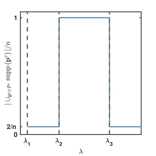
Refer to caption
Figure 1: Normalized cardinality of the broadest support for $\mathbf{p}\in\mathcal{P}^{o}$ versus $\lambda$. The vertical gray dashed lines mark the locations of $\lambda_{1},\lambda_{2}$, and $\lambda_{3}$ that divide the values of $\lambda$ into different regions. For $\lambda\leq\lambda_{2}$ or $\lambda\geq\lambda_{3}$, the normalized cardinality is $2/n$, whereas it is one for $\lambda_{2}<\lambda<\lambda_{3}$. For $\lambda_{2}<\lambda<\lambda_{3}$, the cardinality of the broadest possible support is obtained by testing all the extremum points numerically. The values of other parameters are $k_{1}=30,k_{n}=1$, and $z=15.5$. The values of $\lambda_{i}$ for $i\in\{1\hbox{--}3\}$ are $\lambda_{1}\approx 0.0344$, $\lambda_{2}\approx 0.0709$ and $\lambda_{3}\approx 0.1290$. The support of the degree distribution can take on any integer value between $k_{1}$ and $k_{n}$, i.e., $\mathbf{k}=[30,29,\cdots,1]^{T}$ and $n=30$.

Consider the case where $\lambda$ is slightly above $\lambda_{2}$ and $(k_{1},k_{n})$ is a unique point such that $g(k_{1},k_{n})>0$. From the discussions at the end of Appendix D, we have that, by choosing $k_{i_{1}}=k_{1},k_{i_{3}}=k_{n}$, and $k_{i_{2}}$ to be any allowed degree with $k_{1}>k_{i_{2}}>k_{3}$, the triple $(k_{i_{1}},k_{i_{2}},k_{i_{3}})$ will define a physical degree distribution from Eq. (33). As the middle degree $k_{i_{2}}$ is arbitrary, the broadest support in this case consists of all the allowed degrees in $\mathbf{k}$, i.e., the cardinality of the broadest support increases abruptly from 2 to $n$ at $\lambda=\lambda_{2}$. Similarly, it can be seen that, when $\lambda$ is slightly below $\lambda_{3}$ and $(z^{+},z^{-})$ is the unique point such that $g(z^{+},g^{-})<0$, the broadest support also consists of all the possible nodal degrees. Figure 1 shows the normalized cardinality of the broadest possible support versus $\lambda$. We see that, for $\lambda_{2}<\lambda<\lambda_{3}$, the broadest support indeed consists of all the distinct degrees allowed in $\mathbf{k}$, indicating that, except for relatively low or high values of $\lambda$, the support of the optimal degree distribution can be quite broad.

Refer to caption
Figure 2: Bounds of degree heterogeneity of the optimal degree distributions versus the infection rate. The vertical gray dashed lines mark the locations of $\lambda_{1},\lambda_{2}$, and $\lambda_{3}$ that divide $\lambda$ into different regions. The blue solid trace represents the bounds of the degree heterogeneity $H$. For $\lambda\leq\lambda_{2}$ or $\lambda\geq\lambda_{3}$, the lower and upper bounds coincide. For $\lambda_{2}<\lambda<\lambda_{3}$, the degree heterogeneity can take on any value in the shaded region. Other parameter values are $k_{1}=30$, $k_{n}=1$ and $z=15.5$. The values of $\lambda_{i}$ for $i\in\{1\hbox{--}3\}$ and $n$ are the same as those in Fig. 1.

In general, the degree heterogeneity of a network, defined as $H=\langle k^{2}\rangle/\langle k\rangle^{2}$, can have significant impacts on the spreading dynamics. A natural question is, what is the degree heterogeneity of the optimal degree distribution? Since the average degree is fixed ($\langle k\rangle=z$), the degree heterogeneity determines the outbreak threshold. For sufficiently small values of $\lambda$ where there is a unique network that can trigger an epidemic outbreak, the optimal network structure is one with the largest degree heterogeneity.

Consider the general problem of finding maxima and minima of $H$ among all degree distributions. The extrema of $H$ can be found by maximizing or minimizing the second moment $\langle k^{2}\rangle$ of the degree distribution. The Bhatia-Davis inequality stipulates that the second moment of $\mathbf{p}$ is maximized when it is concentrated at the endpoints $k_{1}$ and $k_{n}$. To minimize the second moment, we note that the definition $\langle k^{2}\rangle=\sum_{i=1}^{n}p_{i}k_{i}^{2}$ has a similar form to Eq. (17) with $\chi_{i}$ replaced by $k_{i}^{2}$. Following the reasoning in Sec. III.2, we see that the minimum of $H$ is supported on two nodal degrees. Through a direct comparison of all distributions supported on two degrees, we find that $H$ is minimized when $\mathbf{p}$ concentrates on $\{z^{+},z^{-}\}$. We see that the optimal degree distributions for $\lambda\leq\lambda_{2}$ and $\lambda\geq\lambda_{3}$ are exactly the ones that maximize and minimize the degree heterogeneity, respectively.
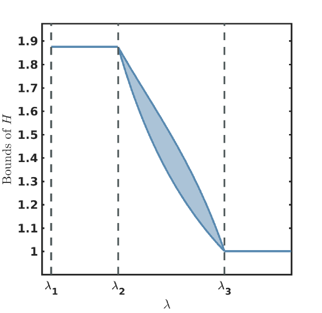
For a fixed $\lambda$ value in the intermediate region ($\lambda_{2}<\lambda<\lambda_{3}$), the values of $H$ for different degree distributions in $\mathcal{P}^{o}$ are not necessarily identical. From Eq. (54), we see that, if $\mathbf{p}$ is a convex combination of the extremum points, its second moment can be obtained by the same convex combination of the second moment of the extremum points. Consequently, the degree heterogeneity of $\mathbf{p}\in\mathcal{P}^{o}$ is bounded by that of the extremum points. Figure 2 shows the bounds of the degree heterogeneity $H$ of the optimal degree distributions versus $\lambda$. The general phenomenon is that the optimal network is more heterogeneous for small infection rates but less so for large rates, as the upper and lower bound of $H$ decreases with $\lambda$. However, the degree heterogeneity does not decrease with $\lambda$ in a strict sense but only trendwise. In fact, if we draw a line segment joining the two degree distributions that reach the upper and lower bounds, then $H$ varies continuously on this line segment, i.e., the degree heterogeneity can take on any value between the lower and upper bounds.

Refer to caption
Figure 3: Spreading prevalence divided by $\lambda z$ versus $\lambda$ for three different degree distributions. The values of the spreading prevalence are obtained by solving the HMF equations numerically. The vertical gray dashed lines mark the locations of $\lambda_{2},(\lambda_{2}+\lambda_{3})/2$, and $\lambda_{3}$ where the three degree distributions are optimal. The horizontal black dashed line correspond to $\psi(\mathbf{p})/\lambda z=1/4$. Other parameter values are $k_{1}=30,k_{n}=1$, and $z=15.5$. The values of $\lambda_{i}$ for $i\in\{1\hbox{--}3\}$ and $n$ are the same as those in Fig. 1.

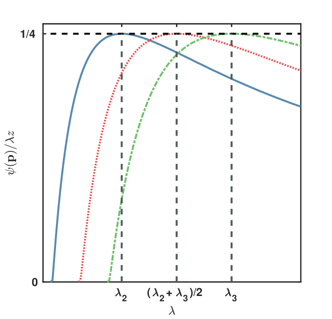
Our analysis of the characteristics of the optimal degree distributions reveals a phenomenon: The existence of a particular value of the infection rate for which every degree distribution is optimal. From the definition of $\mathcal{P}^{o}$, any $\mathbf{p}\in\mathcal{P}^{o}$ must satisfy the first equation in Eq. (25), whose left-hand side is an increasing function of $\lambda$ that converges to zero or $z$ for $\lambda\to 0$ or $\lambda\to\infty$, respectively. As a result, for any $\mathbf{p}\in\mathcal{P}$, there always exists a unique $\lambda$ value such that $\mathbf{p}\in\mathcal{P}^{o}$. Only two degree distributions are optimal under multiple values of $\lambda$, which are the two supported on either $\{k_{1},k_{n}\}$ or $\{z^{+},z^{-}\}$, as they are optimal when $\mathcal{P}^{o}$ is empty. In Sec. III.2, we have shown that for any $\mathbf{p}\notin\mathcal{P}^{o}$, its spreading prevalence is strictly less than $\lambda z/4$. This suggests the following phenomenon: For any degree distributions, its spreading prevalence as a function of $\lambda$ will touch the line $\psi(\mathbf{p})=\lambda z/4$ only at one value of $\lambda$ and under this value of $\lambda$ the degree distribution is among the optimal degree distributions. For all other values of $\lambda$, its spreading prevalence will strictly be below the line $\psi(\mathbf{p})=\lambda z/4$.

To illustrate the phenomenon, we consider three degree distributions that are optimal at $\lambda=\lambda_{2},\lambda=(\lambda_{2}+\lambda_{3})/2$, and $\lambda=\lambda_{3}$, respectively. For $\lambda=\lambda_{2}$ or $\lambda=\lambda_{3}$, the optimal degree distribution is unique. For $\lambda=(\lambda_{2}+\lambda_{3})/2$, we randomly pick a degree distribution from $\mathcal{P}^{o}$ by a uniformly random convex combination of the extremum points. We plot $\psi(\mathbf{p})/\lambda z$ versus $\lambda$ for three degree distributions as shown in Fig. 3. It can be seen that the value of $\psi(\mathbf{p})/\lambda z$ reaches 1/4 at the predicted value of $\lambda$ and is below 1/4 for any other values of $\lambda$.

VI Discussion

Given a dynamical process of interest, identifying the extremum network provides deeper insights into the interplay between network structure and dynamics. From the perspective of applications, searching for a global dynamics-specific optimal network can be valuable in areas such as information diffusion, transportation, and behavior promotion. The issue, however, belongs to the category of dynamics-based inverse problems that are generally challenging and extremely difficult to solve. We have taken an initial step in this direction. Specifically, by limiting the study to SIS type of spreading dynamics and imposing the annealed approximation, we have obtained analytic solutions to the inverse problem. Our solutions unveil a phenomenon with implications: A fundamental characteristic of the optimal network, its degree heterogeneity, depends on the infection rate. In particular, strong degree heterogeneity facilitates the spreading but only for small infection rates. For relatively large infection rates, the optimal structure tends to choose the networks that are less heterogeneous. This means that, when designing an optimal network, e.g., for information spreading, the ease with which information can diffuse among the nodes must be taken into account. Our analysis has also revealed the existence of a particular value of the infection rate for which every degree distribution is globally optimal.

The annealed approximation that serves the base of our analysis is applicable to networks that are describable by the uncorrelated configuration model. It remains to be an open problem to find the optimal quenched networks for SIS dynamics. In Ref. St-Onge et al. (2018), the authors introduced a technique to bridge the annealed and quenched limit of the SIS model. The technique can provide a starting point to extend our analytic approach to quenched networks. The variational analysis in the current paper can be extended to SIS type dynamics on quenched weighted networks to derive a necessary condition for local optimum. In the variational calculus, we have to perform a network structural perturbation to the mean-field equation; therefore, we emphasize a necessary element that makes the variational calculations viable: The spreading prevalence is a continuous function of the perturbations, at least locally around the network being perturbed. The variational analysis will result in a necessary condition for local optimum. However, it is not clear yet what we can derive from the necessary condition without annealed approximations. To generalize the theory to settings under less stringent simplifications is at present an open topic worth investigating. Another assumption in the present paper is that only the number of edges is held fixed, and it is useful to study the optimal networks under more realistic restrictions. Moreover, it is of general interest to seek optimal solutions of network structures for different types of dynamical processes. Our paper represents a step forward in this direction.

Acknowledgments

L.P. would like to acknowledge support from the National Natural Science Foundation of China under Grant No. 62006122. W.W. would like to acknowledge support from the National Natural Science Foundation of China under Grant No. 61903266, Sichuan Science and Technology Program Grant No. 20YYJC4001, China Postdoctoral Science Special Foundation Grant No. 2019T120829, and the Fundamental Research Funds for the central Universities Grant No. YJ201830. L.T. would like to acknowledge support from The Major Program of the National Natural Science Foundation of China under Grant No. 71690242 and the National Key Research and Development Program of China under Grant No. 2020YFA0608601. Y.-C.L. would like to acknowledge support from the Vannevar Bush Faculty Fellowship program sponsored by the Basic Research Office of the Assistant Secretary of Defense for Research and Engineering and funded by the Office of Naval Research through Grant No. N00014-16-1-2828.

Appendix A Proof that $\mathbf{x}^{*}$ is a continuously differentiable function of $\mathbf{p}$ above the outbreak threshold

Setting the right-hand side of Eq. (1) to zero for an equilibrium, we get

$$x^{*}_{i}=\frac{\lambda k_{i}\Theta^{*}}{1+\lambda k_{i}\Theta^{*}},$$ (56)

where $\Theta^{*}$ is obtained by substituting $\mathbf{x}(t)=\mathbf{x}^{*}$ into Eq. (2). Define a function $f(\mathbf{p},\mathbf{x}):(\mathbf{p},\mathbf{x})\to\mathbb{R}^{n}$ as

$$f_{i}(\mathbf{p},\mathbf{x})=x_{i}-\frac{\lambda k_{i}\sum_{l=1}^{n}p_{l}k_{l}x_{l}}{z+\lambda k_{i}\sum_{l=1}^{n}p_{l}k_{l}x_{l}},$$ (57)

we have $f(\mathbf{p},\mathbf{x}^{*})=0$. Note that $f(\mathbf{p},\mathbf{x})$ is a continuously differentiable function of $\mathbf{p}$ and $\mathbf{x}$. We now show that, from the relation $f(\mathbf{p},\mathbf{x}^{*})=0$, the stable equilibrium point $\mathbf{x}^{*}$ can be written as a continuously differentiable function of $\mathbf{p}$ for $\lambda>z/\langle k^{2}\rangle$ by applying the implicit function theorem.

The derivative of $f_{i}(\mathbf{p},\mathbf{x})$ with respect to $x_{j}$ is

$$\frac{\partial f_{i}(\mathbf{p},\mathbf{x})}{\partial x_{j}}=\delta_{i,j}-\frac{\lambda zk_{i}k_{j}p_{j}}{\left(z+\lambda k_{i}\sum_{l=1}^{n}p_{l}k_{l}x_{l}\right)^{2}},$$ (58)

where $\delta_{i,j}$ is the Kronecker $\delta$. The Jacobian matrix of $f(\mathbf{p},\mathbf{x})$ to $\mathbf{x}$ can be written as $\mathcal{I}-\mathbf{r}\mathbf{s}^{T}$, where $\mathcal{I}$ is the $n\times n$ identity matrix and $\mathbf{r}$ and $\mathbf{s}$ are $n\times 1$ vectors with elements,

$$r_{i}=\frac{\lambda zk_{i}}{\left(z+\lambda k_{i}\sum_{l=1}^{n}p_{l}k_{l}x_{l}\right)^{2}},\qquad s_{i}=k_{i}p_{i}.$$ (59)

Let $\mathbf{b}$ be an eigenvector of the matrix $\mathbf{r}\mathbf{s}^{T}$ with eigenvalue $\omega$. From the eigenvalue equation, we have

$$\sum_{j=1}^{n}r_{i}s_{j}b_{j}=\omega b_{i}.$$ (60)

Multiplying both sides by $s_{i}$ and summing over $i$, we have

$$\sum_{i=1}^{n}r_{i}s_{i}\sum_{j=1}^{n}s_{j}b_{j}=\omega\sum_{i=1}^{n}s_{i}b_{i}.$$ (61)

As a result, the only possible eigenvalues of matrix $\mathbf{r}\mathbf{s}^{T}$ are $\omega=0$ or $\omega=\sum_{i=1}^{n}r_{i}s_{i}$.

For $\lambda>z/\langle k^{2}\rangle$, all elements of $\mathbf{x}^{*}$ are positive. At $\mathbf{x}=\mathbf{x}^{*}$, we have

$$\begin{split}\sum_{i=1}^{n}r_{i}s_{i}=&\sum_{i=1}^{n}\frac{\lambda zp_{i}k_{i}^{2}}{\left(z+\lambda k_{i}\sum_{l=1}^{n}p_{l}k_{l}x^{*}_{l}\right)^{2}}\\ =&\frac{1}{z}\sum_{i=1}^{n}\lambda p_{i}k_{i}^{2}(1-x^{*}_{i})^{2}\\ =&\frac{1}{z\Theta^{*}}\sum_{i=1}^{n}p_{i}k_{i}x^{*}_{i}(1-x^{*}_{i})\\ =&1-\frac{1}{z\Theta^{*}}\sum_{i=1}^{n}p_{i}k_{i}\left(x^{*}_{i}\right)^{2}<1,\end{split}$$ (62)

where the second and third equalities can be verified by substituting them into Eq. (56) and $x^{*}_{i}=\lambda k_{i}(1-x^{*}_{i})\Theta^{*}$, respectively.

Taken together, the eigenvalues of the matrix $\mathbf{r}\mathbf{s}^{T}$ are less than one for $\lambda>z/\langle k^{2}\rangle$, so the eigenvalues of the Jacobian matrix $\mathcal{I}-\mathbf{r}\mathbf{s}^{T}$ are less than zero, which further implies that the Jacobian matrix is invertible. By the implicit function theorem, $\mathbf{x}^{*}$ is a continuously differentiable function of $\mathbf{p}$.

Appendix B Eigenvalues of the Jacobian matrix

Denote the right side of Eq. (1) by

$$h_{i}=-x_{i}(t)+\lambda k_{i}\left[1-x_{i}(t)\right]\Theta.$$ (63)

The Jacobian matrix for $h=\left(h_{1},\cdots,h_{n}\right)^{T}$ at $\mathbf{x}=\mathbf{x}^{*}$ is exactly $\mathcal{J}$: $\nabla h=\mathcal{J}$. As $\mathbf{x}^{*}$ is the unique global stable equilibrium point Wang and Dai (2008), the eigenvalues of $\mathcal{J}$ must have negative real parts.

Appendix C Detailed derivation of $\mathbf{\chi}$

Define two vectors $\mu$ and $\nu$ of length $n$ whose elements are

$$\mu_{i}=\frac{\lambda}{z}k_{i}\left(1-x^{*}_{i}\right),\qquad\nu_{i}=k_{i}p_{i}.$$ (64)

Further, define a $n\times n$ diagonal matrix $\mathcal{D}$ with the elements

$$D_{ii}=-1-\lambda k_{i}\Theta^{*}.$$ (65)

By the Sherman-Morrison formula, we have

$$\begin{split}&\mathcal{J}^{-1}=\left(\mathcal{D}+\mu\cdot\nu^{T}\right)^{-1}=\mathcal{D}^{-1}-\frac{\mathcal{D}^{-1}\cdot\mu\cdot\nu^{T}\cdot\mathcal{D}^{-1}}{1+\nu^{T}\cdot\mathcal{D}^{-1}\mu}.\end{split}$$ (66)

Substituting Eq. (14) into Eq. (16), we get Eq. (17) with $\chi_{i}$ given by

$$\chi_{i}=x^{*}_{i}-k_{i}x^{*}_{i}p^{T}\mathcal{J}^{-1}\mu.$$ (67)

Inserting Eq. (66) into Eq. (67) leads to

$$\begin{split}&\chi_{i}=x^{*}_{i}\\ &+\frac{\lambda k_{i}x_{i}\sum_{j=1}^{n}p_{j}k_{j}(1-x^{*}_{j})\left(1+\lambda k_{j}\Theta^{*}\right)^{-1}}{z-\lambda\sum_{j=1}^{n}p_{j}k^{2}_{j}(1-x^{*}_{j})\left(1+\lambda k_{j}\Theta^{*}\right)^{-1}}.\end{split}$$ (68)

At the equilibrium point, we have

$$-x^{*}_{i}+\lambda k_{i}\left(1-x^{*}_{i}\right)\Theta^{*}=0,$$ (69)

which leads to

$$\left(1+\lambda k_{j}\Theta^{*}\right)^{-1}=\left(1-x^{*}_{i}\right).$$ (70)

Substituting the above two equations into Eq. (68), we obtain

$$\chi_{i}=x^{*}_{i}\left(1+\frac{\lambda k_{i}\Theta^{*}\sum_{j=1}^{n}p_{j}k_{j}(1-x^{*}_{j})^{2}}{\sum_{j=1}^{n}p_{j}k_{j}(x^{*}_{j})^{2}}\right),$$ (71)

which is Eq. (18).

Appendix D Conditions for $\mathbf{\mathcal{P}^{o}}$ to be nonempty

We test the validity of the three inequalities in (35) in a sequential manner: First we study the condition for $\lambda$ when there exist $k_{i_{1}}$ and $k_{i_{3}}$ such that $g(k_{i_{1}},k_{i_{3}})\geq 0$ holds, we then test under the derived condition if there exists $k_{i_{2}}$ such that the other two inequalities hold.

As a preparation, we prove a result that will be used repeatedly in the rest of this appendix. In particular, we show that for $\mathcal{P}^{o}$ to be nonempty, it is necessary to have $\lambda z\leq 2$ from Eq. (26). Note that Eq. (26) is the average of the function $f(k_{a})=2k_{a}/(2+\lambda k_{a})$ under the degree distribution $\mathbf{p}$. This function has a negative second order derivative $f^{\prime\prime}(k_{a})=-8\lambda/(2+\lambda k_{a})^{3}$, so $f(k_{a})$ is concave. By Jensen’s inequality, we have

$$\sum_{i=1}^{n}p_{i}\frac{2k_{i}}{2+\lambda k_{i}}\leq\frac{2z}{2+\lambda z}.$$ (72)

Since the left side equals $z/2$ from Eq. (26), it is necessary to have $2z/(2+\lambda z)\geq z/2$, which implies $\lambda z\leq 2$. The equality in Eq. (72) holds only when $z$ is an integer and is one of the allowed degrees in $\mathbf{k}$ and, in addition, $\mathbf{p}$ concentrates on $z$. In this case we have $\lambda z=2$, so $\mathcal{P}^{o}$ has a unique element $p$ that concentrates on $z$.

We consider the case of $\lambda z<2$. The analysis begins with the setting of the existence of $(k_{i_{1}},k_{i_{3}})$ such that $g(k_{i_{1}},k_{i_{3}})\geq 0$ holds. Defining $z^{+}=\mathrm{min}_{i}\{k_{i}\geq z\}$ and $z^{-}=\mathrm{max}_{i}\{k_{i}\leq z\}$, we have $k_{i_{1}}\in\{k_{1},k_{2},\cdots,z^{+}\}$ and $k_{i_{3}}\in\{z^{-},\cdots,k_{n-1},k_{n}\}$. The function $g(k_{a},k_{b})$ is quadratic in $\lambda$, and the equation $g(k_{a},k_{b})=0$ has two roots: one positive and one negative. The positive one is

$$\lambda^{(k_{a},k_{b})}=\frac{2}{z}-\frac{1}{k_{a}}-\frac{1}{k_{b}}+\sqrt{\left(\frac{1}{k_{a}}+\frac{1}{k_{b}}-\frac{2}{z}\right)^{2}+\frac{4}{k_{a}k_{b}}}.$$ (73)

As a result, for $0<\lambda<\lambda^{(k_{a},k_{b})}$, we have $g(k_{a},k_{b})<0$, whereas $g(k_{a},k_{b})\geq 0$ for $\lambda\geq\lambda^{(k_{a},k_{b})}$. If $\lambda^{(k_{a},k_{b})}$ is regarded as a function of $k_{a}$ and $k_{b}$, through the derivatives, we have that $\lambda^{(k_{a},k_{b})}$ is a decreasing function of $k_{a}$ for $k_{a}>z$ and an increasing function of $k_{b}$ for $k_{b}<z$. Consequently, the value of $\lambda^{(k_{a},k_{b})}$ reaches its minimum at $(k_{1},k_{n})$. There exists at least one $(k_{i_{1}},k_{i_{3}})$ such that $g(k_{i_{1}},k_{i_{3}})\geq 0$ insofar as $\lambda\geq\lambda^{(k_{1},k_{n})}$.

Having determined the condition under which there exists $(k_{i_{1}},k_{i_{3}})$ such that $g(k_{i_{1}},k_{i_{3}})\geq 0$ holds, we can obtain the conditions under which there exists $k_{i_{2}}$ such that $g(k_{i_{1}},k_{i_{2}})\leq 0$ and $g(k_{i_{2}},k_{i_{3}})\leq 0$. When the curve $g(k_{a},k_{b})=0$ passes an integer point that can be chosen as $(k_{i_{1}},k_{i_{3}})$, we have $g(k_{i_{1}},k_{i_{3}})=0$. From Eq. (33), we have $p_{i_{2}}=0$ and

$$p_{i_{1}}=\frac{z-k_{i_{3}}}{k_{i_{1}}-k_{i_{3}}},\qquad p_{i_{3}}=\frac{k_{i_{1}}-z}{k_{i_{1}}-k_{i_{3}}}.$$ (74)

We see that $p_{i_{1}}$ and $p_{i_{3}}$ are independent of the choice of $k_{i_{2}}$ and $\mathbf{p}$ is supported on one or two nodal degrees.

Now consider the case of $g(k_{i_{1}},k_{i_{3}})>0$. For fixed $(k_{i_{1}},k_{i_{3}})$, the inequalities $g(k_{i_{1}},k_{i_{2}})\leq 0$ and $g(k_{i_{2}},k_{i_{3}})\leq 0$ can be rearranged as

$$\begin{split}&\left[\left(4\lambda-\lambda^{2}z\right)k_{i_{1}}-2\lambda z\right]k_{i_{2}}\geq 2\lambda zk_{i_{1}}-4z,\\ &\left[\left(4\lambda-\lambda^{2}z\right)k_{i_{3}}-2\lambda z\right]k_{i_{2}}\geq 2\lambda zk_{i_{3}}-4z.\end{split}$$ (75)

As $k_{i_{1}}\geq z$ and $\lambda z<2$, we have

$$\left(4\lambda-\lambda^{2}z\right)k_{i_{1}}-2\lambda z>0.$$ (76)

From $g(k_{i_{1}},k_{i_{3}})\geq 0$ we have

$$\left(\left(4\lambda-\lambda^{2}z\right)k_{i_{3}}-2\lambda z\right)k_{i_{1}}\leq 2\lambda zk_{i_{3}}-4z.$$ (77)

Because $\lambda z<2$ and $k_{i_{3}}\leq z$, the right-hand side of the above inequality is negative. We, thus, have

$$\left(4\lambda-\lambda^{2}z\right)k_{i_{3}}-2\lambda z<0.$$ (78)

With the above results, Eq. (75) implies that there exist feasible values of $k_{i_{2}}$ insofar as

$$\frac{2\lambda zk_{i_{1}}-4z}{\left(4\lambda-\lambda^{2}z\right)k_{i_{1}}-2\lambda z}\leq\frac{2\lambda zk_{i_{3}}-4z}{\left(4\lambda-\lambda^{2}z\right)k_{i_{3}}-2\lambda z}$$ (79)

and there is at least one integer between the two sides of the inequality.

Defining a function of $\lambda$ and $k_{a}$ as

$$f(\lambda,k_{a})=\frac{2\lambda zk_{a}-4z}{\left(4\lambda-\lambda^{2}z\right)k_{a}-2\lambda z},$$ (80)

we have that the left and right sides of Eq. (79) are equal to $f(\lambda,k_{i_{1}})$ and $f(\lambda,k_{i_{3}})$, respectively. The derivative of $f(k_{a})$ with respect to $k_{a}$ is

$$\frac{\partial f(\lambda,k_{a})}{\partial k_{a}}=\frac{8\lambda z\left(2-\lambda z\right)}{\left(\left(4\lambda-\lambda^{2}z\right)k_{a}-2\lambda z\right)^{2}}.$$ (81)

Consequently, $f(\lambda,k_{a})$ is an increasing function of $k_{a}$ for $\lambda z<2$ and the function is non-singular, so $f(\lambda,k_{i_{1}})$ is bounded from above as

$$f(\lambda,k_{i_{1}})<\lim_{k_{a}\to\infty}f(k_{a})=\frac{2z}{4-\lambda z}<z,$$ (82)

whereas $f(\lambda,k_{i_{3}})$ is bounded from below as

$$f(\lambda,k_{i_{3}})>\lim_{k_{a}\to 0}f(k_{a})=\frac{2}{\lambda}>z.$$ (83)

We thus have that the inequality $f(\lambda,k_{i_{1}})<f(\lambda,k_{i_{3}})$ holds for $\lambda z<2$. It remains to determine if there is an integer between $f(\lambda,k_{i_{1}})$ and $f(\lambda,k_{i_{3}})$. In this regard, if $z$ is an integer and is one of the degrees allowed, the situation is relatively simple, and we pick $k_{i_{2}}=z$.

We analyze the case where $z$ is not an integer. Note that the left-hand side of Eq. (79) is strictly less than the right-hand side and $f(\lambda,k_{a})$ is an increasing function of $k_{a}$. The gap between the two sides of Eq. (79) is then maximized for $(k_{i_{1}},k_{i_{3}})=(z^{+},z^{-})$. Suppose there are no integer points between $f(\lambda,z^{+})$ and $f(\lambda,z^{-})$. It implies that there are no integer points between $f(\lambda,k_{i_{1}})$ and $f(\lambda,k_{i_{3}})$ for any other choice of $(k_{i_{1}},k_{i_{3}})$. For $\lambda=\lambda^{(z^{+},z^{-})}$, the curve $g(k_{a},k_{b})=0$ passes the point $(k_{a},k_{b})=(z^{+},z^{-})$ and set $\mathcal{P}^{o}$ is nonempty based on Eq. (74), as we can take $(k_{i_{1}},k_{i_{3}})=(z^{+},z^{-})$. In the next, we show that if $\lambda>\lambda^{(z^{+},z^{-})}$, set $\mathcal{P}^{o}$ will be empty as there are no integer points between $f(\lambda,z^{+})$ and $f(\lambda,z^{-})$. However, for $\lambda<\lambda^{(z^{+},z^{-})}$, $\mathcal{P}^{o}$ is guaranteed to be nonempty.

To show that $\mathcal{P}^{o}$ is empty for $\lambda>\lambda^{(z^{+},z^{-})}$, we note that the derivative of $f(\lambda,k_{a})$ with respect to $\lambda$ is

$$\frac{\partial f(\lambda,k_{a})}{\partial\lambda}=\frac{2z^{2}\left(\lambda k_{a}-2\right)^{2}+16z\left(k_{a}-z\right)}{\left[\left(4\lambda-\lambda^{2}z\right)k_{a}-2\lambda z\right]^{2}}.$$ (84)

For $k_{a}\geq z$ and $\lambda z<2$, the derivative is positive, so $f(\lambda,k_{a})$ is an increasing function of $\lambda$. Now we show that if

$$\left(4\lambda-\lambda^{2}z\right)k_{a}-2\lambda z<0,$$ (85)

then $f(\lambda,k_{a})$ is a decreasing function of $\lambda$. Note that $k_{i_{3}}$ satisfies the above inequality for $g(k_{i_{1}},k_{i_{3}})>0$ [c.f., the discussions above Eq. (79)]. Taking the derivative with respect to $k_{a}$ for the numerator of the right-hand side of Eq. (84), we get

$$4\lambda z^{2}(\lambda k_{a}-2)+16z>16z-8\lambda z^{2}>0,$$ (86)

where the second inequality is the result of applying $\lambda z<2$. The numerator on the right side of Eq. (84) itself is an increasing function of $k_{a}$. In addition, Eq. (85) implies

$$k_{a}<\frac{2z}{4-\lambda z}.$$ (87)

When $k_{a}$ equals the right side of this inequality, the numerator of the right side of Eq. (84) becomes,

$$\frac{16\lambda z^{3}(\lambda z-2)}{(4-\lambda z)^{2}}<0,$$ (88)

so $f(\lambda,k_{a})$ is a decreasing function of $\lambda$ when Eq. (85) holds. For $\lambda=\lambda^{(z^{+},z^{-})}$, we have $f(\lambda,z^{+})=z^{-}$ and $f(\lambda,z^{-})=z^{+}$. For $\lambda>\lambda^{(z^{+},z^{-})}$, the left side of Eq. (79) increases from $z^{-}$ whereas the right side decreases from $z^{+}$. As a result, the gap between the two sides becomes smaller, and there cannot be any integer point in between.

We now show that, for $\lambda^{(k_{1},k_{n})}<\lambda<\lambda^{(z^{+},z^{-})}$, set $\mathcal{P}^{o}$ is guaranteed to be nonempty. In this region of $\lambda$, we have $g(k_{1},k_{n})>0$ and $g(z^{+},z^{-})<0$. Consider the point $(k_{a},k_{b})=(z^{+},k_{n})$. For $g(z^{+},k_{n})=0$, according to Eq. (74), set $\mathcal{P}^{o}$ is nonempty. The other two possibilities: $g(z^{+},k_{n})>0$ and $g(z^{+},k_{n})<0$, can be treated separately. Suppose $g(z^{+},k_{n})>0$, we can pick $k_{i_{1}}=z^{+},k_{i_{2}}=z^{-}$ and $k_{i_{3}}=k_{n}$. In this case, $g(k_{i_{1}},k_{i_{2}})<0$ and $g(k_{i_{1}},k_{i_{3}})>0$ hold by definition. It can then be shown that these two inequalities imply $g(k_{i_{2}},k_{i_{3}})<0$. In particular, note that

$$\begin{split}&g(k_{i_{2}},k_{i_{3}})-g(k_{i_{1}},k_{i_{2}})\\ =&\left(k_{i_{1}}-k_{i_{3}}\right)\left(\left(4\lambda-\lambda^{2}z\right)k_{i_{2}}-2\lambda z\right).\end{split}$$ (89)

As $g({k_{i_{1}},k_{i_{2}}})<0$, we have

$$\left(\left(4\lambda-\lambda^{2}z\right)k_{i_{2}}-2\lambda z\right)k_{i_{1}}<2\lambda zk_{i_{2}}-4z.$$ (90)

Since $k_{i_{2}}=z^{-}\leq z$ and $\lambda z<2$, the right side is negative and we have $\left(\left(4\lambda-\lambda^{2}z\right)k_{i_{2}}-2\lambda z\right)<0$. This implies $g(k_{i_{2}},k_{i_{3}})<g(k_{i_{1}},k_{i_{2}})<0$. For the other case of $g(z^{+},k_{n})<0$, we pick $k_{i_{1}}=k_{1}$, $k_{i_{2}}=z^{+}$ and $k_{i_{3}}=k_{n}$, so $g(k_{i_{2}},k_{i_{3}})<0$ and $g(k_{i_{1}},k_{i_{3}})>0$ hold by definition. From $\lambda z<2$ and $k_{i_{2}}=z^{+}\geq z$, we have $\left(\left(4\lambda-\lambda^{2}z\right)k_{i_{2}}-2\lambda z\right)>0$. It can thus be concluded from Eq. (89) that $0>g(k_{i_{2}},k_{i_{3}})>g(k_{i_{1}},k_{i_{2}})$.

The above proof procedure can be applied to the case of picking $(k_{i_{1}},k_{i_{2}},k_{i_{3}})$ for $\lambda^{(k_{1},k_{n})}<\lambda<\lambda^{(z^{+},z^{-})}$. Suppose there are four degrees $k_{a}>k_{b}>z>k_{c}>k_{d}$, with $g(k_{a},k_{d})<0$ and $g(k_{b},k_{c})>0$. If the point $(k_{b},k_{d})$ has $g(k_{b},k_{d})>0$, we have that $(k_{i_{1}},k_{i_{2}},k_{i_{3}})=(k_{b},k_{c},k_{d})$ defines a physical degree distribution from Eq. (33). Similarly, if $g(k_{a},k_{c})<0$, we can choose $(k_{i_{1}},k_{i_{2}},k_{i_{3}})=(k_{a},k_{b},k_{c})$.

The results of this appendix can be summarized as follows. Let $\lambda_{2}=\lambda^{(k_{1},k_{n})}$ and $\lambda_{3}=\lambda^{(z^{+},z^{-})}$. For $\lambda_{1}<\lambda<\lambda_{2}$, the set $\mathcal{P}^{o}$ is empty and we can only find the local maxima among all degree distributions that are supported on one or two nodal degrees. For $\lambda_{2}\leq\lambda\leq\lambda_{3}$, set $\mathcal{P}^{o}$ is nonempty, and it is necessary to further analyze if there are other local maxima supported on one or two nodal degrees and if the degree distributions in $\mathcal{P}^{o}$ are maxima and global maxima. For $\lambda>\lambda_{3}$, set $\mathcal{P}^{o}$ again becomes empty.

Appendix E Solution of the HMF equation for degree distribution supported on two nodal degrees

The equilibrium point $\mathbf{x}^{*}$ is given by the solution of

$$\lambda k_{i_{1}}(1-x^{*}_{i_{1}})\Theta^{*}=x^{*}_{i_{1}},\ \lambda k_{i_{2}}(1-x^{*}_{i_{2}})\Theta^{*}=x^{*}_{i_{2}}.$$ (91)

Multiplying the two equations in Eq. (91) by $p_{i_{1}}$ and $p_{i_{2}}$, respectively, and summing them, we obtain

$$\psi(\mathbf{p})=\lambda z\Theta^{*}-\lambda z\left(\Theta^{*}\right)^{2}.$$ (92)

To obtain $\psi(\mathbf{p})$, it suffices to find the value of $\Theta^{*}$.

Equation (91) gives

$$x^{*}_{i_{1}}=\frac{\lambda k_{i_{1}}\Theta^{*}}{1+\lambda k_{i_{1}}\Theta^{*}},\ x^{*}_{i_{2}}=\frac{\lambda k_{i_{2}}\Theta^{*}}{1+\lambda k_{i_{2}}\Theta^{*}}.$$ (93)

From the definition of $\Theta^{*}$, we have

$$\begin{split}z\Theta^{*}=p_{i_{1}}k_{i_{1}}x^{*}_{i_{1}}+p_{i_{2}}k_{i_{2}}x^{*}_{i_{1}}.\end{split}$$ (94)

Substituting Eq. (93) and the values $p_{i_{1}}$ and $p_{i_{2}}$ in Eq. (38) into Eq. (94), we obtain the following quadratic equation for $\Theta^{*}$:

$$\beta_{2}\left(\Theta^{*}\right)^{2}+\beta_{1}\Theta^{*}+\beta_{0}=0,$$ (95)

with the coefficients,

$$\begin{split}&\beta_{2}=\lambda^{2}zk_{i_{1}}k_{i_{2}},\\ &\beta_{1}=\lambda z\left(k_{i_{1}}+k_{i_{2}}-\lambda k_{i_{1}}k_{i_{2}}\right),\\ &\beta_{0}=z-\lambda zk_{i_{1}}-\lambda zk_{i_{2}}+\lambda k_{i_{1}}k_{i_{2}}.\end{split}$$ (96)

Noting that the second moment of the degree distribution is

$$\langle k^{2}\rangle=p_{i_{1}}k_{i_{1}}^{2}+p_{i_{2}}k_{i_{2}}^{2}=z\left(k_{i_{1}}+k_{i_{2}}\right)-k_{i_{1}}k_{i_{2}},$$ (97)

We have $\beta_{0}=z-\lambda\langle k^{2}\rangle<0$ as $\lambda$ is above the epidemic outbreak threshold $z/\langle k^{2}\rangle$. Since $\beta_{2}>0$, the only physical solution (with $0<\Theta^{*}<1$) of Eq. (95) is

$$\Theta^{*}=\frac{-\beta_{1}+\sqrt{\beta_{1}^{2}-4\beta_{2}\beta_{0}}}{2\beta_{2}}.$$ (98)

Substituting Eq. (98) into Eq. (92), we obtain the value of $\psi(\mathbf{p})$ as given by Eq. (39).

References

  • Aguirre et al. (2013) J. Aguirre, D. Papo,  and J. M. Buldú, “Successful strategies for competing networks,” Nat. Phys. 9, 230 (2013).
  • Pan et al. (2019) L. Pan, W. Wang, S. Cai,  and T. Zhou, “Optimal interlayer structure for promoting spreading of the susceptible-infected-susceptible model in two-layer networks,” Phys. Rev. E 100, 022316 (2019).
  • Pastor-Satorras et al. (2015) R. Pastor-Satorras, C. Castellano, P. Van Mieghem,  and A. Vespignani, “Epidemic processes in complex networks,” Rev. Mod. Phys. 87, 925 (2015).
  • Castellano et al. (2009) C. Castellano, S. Fortunato,  and V. Loreto, “Statistical physics of social dynamics,” Rev. Mod. Phys. 81, 591 (2009).
  • Pastor-Satorras and Vespignani (2001) R. Pastor-Satorras and A. Vespignani, “Epidemic dynamics and endemic states in complex networks,” Phys. Rev. E 63, 066117 (2001).
  • Cohen et al. (2003) R. Cohen, S. Havlin,  and D. ben-Avraham, “Efficient immunization strategies for computer networks and populations,” Phys. Rev. Lett. 91, 247901 (2003).
  • Pastor-Satorras and Vespignani (2002) R. Pastor-Satorras and A. Vespignani, “Immunization of complex networks,” Phys. Rev. E 65, 036104 (2002).
  • Kitsak et al. (2010) M. Kitsak, L. K. Gallos, S. Havlin, F. Liljeros, L. Muchnik, H. E. Stanley,  and H. A. Makse, “Identification of influential spreaders in complex networks,” Nat. Phys. 6, 888 (2010).
  • Lü et al. (2016) L. Lü, D. Chen, X.-L. Ren, Q.-M. Zhang, Y.-C. Zhang,  and T. Zhou, “Vital nodes identification in complex networks,” Phys. Rep. 650, 1 (2016).
  • Valente (2012) T. W. Valente, “Network interventions,” Science 337, 49 (2012).
  • Goel et al. (2016) S. Goel, A. Anderson, J. Hofman,  and D. J. Watts, “The structural virality of online diffusion,” Management Sci. 62, 180 (2016).
  • Ferrara et al. (2016) E. Ferrara, O. Varol, C. Davis, F. Menczer,  and A. Flammini, “The rise of social bots,” Commun. ACM 59, 96 (2016).
  • Vosoughi et al. (2018) S. Vosoughi, D. Roy,  and S. Aral, “The spread of true and false news online,” Science 359, 1146 (2018).
  • Musco et al. (2018) C. Musco, C. Musco,  and C. E. Tsourakakis, “Minimizing polarization and disagreement in social networks,” in Proceedings of the 2018 World Wide Web Conference (2018) pp. 369–378.
  • Wang and Dai (2008) L. Wang and G.-Z. Dai, “Global stability of virus spreading in complex heterogeneous networks,” SIAM J. Appl. Math. 68, 1495 (2008).
  • St-Onge et al. (2018) G. St-Onge, J.-G. Young, E. Laurence, C. Murphy,  and L. J. Dubé, “Phase transition of the susceptible-infected-susceptible dynamics on time-varying configuration model networks,” Phys. Rev. E 97, 022305 (2018).