Analytically solvable model to the spin Hall effect with Rashba and Dresselhaus spin-orbit couplings

Abstract

When the Rashba and Dresslhaus spin-orbit coupling are both presented for a two-dimensional electron in a perpendicular magnetic field, a striking resemblance to anisotropic quantum Rabi model in quantum optics is found. We perform a generalized Rashba coupling approximation to obtain a solvable Hamiltonian by keeping the nearest-mixing terms of Laudau states, which is reformulated in the similar form to that with only Rashba coupling. Each Landau state becomes a new displaced-Fock state with a displacement shift instead of the original Harmonic oscillator Fock state, yielding eigenstates in closed form. Analytical energies are consistent with numerical ones in a wide range of coupling strength even for a strong Zeeman splitting. In the presence of an electric field, the spin conductance and the charge conductance obtained analytically are in good agreements with the numerical results. As the component of the Dresselhaus coupling increases, we find that the spin Hall conductance exhibits a pronounced resonant peak at a larger value of the inverse of the magnetic field. Meanwhile, the charge conductance exhibits a series of plateaus as well as a jump at the resonant magnetic field. Our method provides an easy-to-implement analytical treatment to two-dimensional electron gas systems with both types of spin-orbit couplings.

I Introduction

Spin-orbit coupling (SOC) enables a wide variety of fascinating phenomena, which brings out a new growing research field of spin-orbitronics, a branch of spintronics that focuses on the manipulation of the electron spin degree of freedom Fabian ; Chappert . A prominent example is the spin Hall effect, which is the conversion of a spin unpolarized charge current into a net spin current without charge flow Dyakonov ; Hirsch . It has been discussed intensively zhang2003 ; niu2004 ; NiuRMP ; Kato ; Wunder ; Wunderlich ; Valenzuela ; JairoRMP , in which an electric field induces a transverse spin current. In the presence of a perpendicular magnetic field, the interplay of Zeeman coupling and various spin-orbit interactions has stimulated a lot of discussions on resonance spin Hall conductance shen2004 ; tagliacozzo2008 ; engel07 , which may has potential applications in spintronics.

There are basically two types of SOCs in nature, i.e., the Rashba term with structural inversion asymmetry rashba1960 and the Dresselhaus term due to the bulk inversion asymmetry dresselhaus1955 or interface inversion asymmetry IIA . Usually, both types of SOC coexist in a material, such as GaAs-AlGaAs quantum wells and heterostructures jusserand ; kim2016 ; ishizaka2011 ; Manchon2015 ; lommer1988 ; tretyak2001 , but which one plays a major part depends on the properties of the material. It has been recognized that Rashba and Dresselhaus SOC can interfere with each other, and leads to a number of interesting phenomenon by tuning the ratio between them, such as anisotropic transport loss2003 , spin splitting ganichev04 ; averkiev1999 , control of spin precession park2020 and light scattering gelfert2020 . It has been applied experimentally by various ways, such as external electric field, changing temperature, or inserting extra layer etc Ohno ; Karimov ; Dhrmann ; Belkov ; Muller ; Balocchi ; Hern .

In previous work, many efforts have been devoted to the spin Hall effect with the Rashba SOC in two-dimensional electron gas systems ($2$DEGs), which is caused by the Laudau level crossing near the Fermi energy. A zero-field spin splitting induced by the Rashba SOC competes with the Zeeman splitting in presence of a magnetic field, and then compromise a resonant spin Hall effect at certain magnetic field nitta1997 ; heida1998 . In contrast, Dresselhaus SOC enhances the Zeeman splitting and results in a suppression to the resonance shen05 . There is an analytical solution for the system with only either Rashba or Dresselhaus coupling shen05 ; chang06 . While considering both of them together, an analytical solution is currently not available due to the absence of a full closed-form solution. The perturbation method has been adopted to give rise to an approximated results, which is valid a small ratio of the Zeeman energy to the cyclotron frequency shen05 ; sun2013 . To pursue the intrinsic spin Hall effect induced by the coexistence of the Dresselhaus and Rashba SOCs, it is desirable to develop theories which can solve systems including both types of the SOCs.

In this work we develop a generalized Rashba SOC approximation (GRSOCA) to give an analytical solution to the $2$DEGs with both the Rashba and Dresselhaus SOCs in a magnetic field. Using a displacement transformation and an expansion of even and odd functions of Laudau states up to the nearest-mixing terms, a reformulated Hamiltonian of the same form as that with only Rashba term is obtained, resulting in eigenstates in closed form in the transformed displaced-Fock subspace. The novel displaced-Fock state for each Landau level involves the mixing of infinite Laudau level states induced by two types of SOCs, exhibiting an improvement over original Fock states. Energy levels are obtained explicitly for arbitrary strengths of both types of SOCs, which agree well with numerical results in a wide range of coupling strength even for a strong Zeeman energy. By comparing to the system with only Rashba SOC, we find that the spin Hall conductance exhibits a pronounced resonant peak at a larger value of the inverse of the magnetic field, which arises from the contributions of the Dresselhaus SOC. Resonance originates from the energy degeneracy near Fermi energy, where the eigenstates consist of the $n$th displaced-Fock state of spin up and $n+1$th displaced-Fock state of spin down. A series of plateaus of the charge conductance are observed, and a jump occurs at the resonant point, which fit well with the numerical ones.

The paper is outlined as follows. In Sec. II, we derive expressions for the quantized Hamiltonian of the $2$DEGs with the Rashba and Dresselhaus SOC in a magnetic field. In Sec. III, we obtain the analytical solution of the effective Hamiltonian for arbitrary ratio between the Rashba and Dresselhaus SOCs. In Sec. IV, we study the charge and spin Hall conductances analytically with the first-order corrections when an electric field is applied. Finally, a brief summary is given in Sec. V.

II Hamiltonian

We consider a single electron in a two-dimensional system subjected to a perpendicular magnetic field $\vec{B}=-B\hat{e}_{z}=\nabla\times\vec{A}$, which is confined in the $x-y$ plane of an area $L_{x}\times L_{y}$. The Hamiltonian in the presence of spin-orbit coupling is given by ($\hbar=1$)

$$H_{0}=\frac{1}{2m}(\vec{p}+\frac{e}{c}\vec{A})^{2}-\frac{1}{2}g\mu_{B}B\sigma_{z}+H_{so},$$ (1)

where $g$ is the Lande factor of the electron with the effective mass $m$, $\mu_{B}$ is the Bohr magneton, and $\sigma_{k}$ are the Pauli matrices. The Laudau gauge is chosen as $\vec{A}=B\vec{r}\times\hat{e}_{z}=(yB,0,0)$. The spin-orbit Hamiltonian includes the Rashba SOC and the linear Dresselhaus SOC, $H_{so}=H_{D}+H_{R}$ with $H_{R}=\alpha(\Pi_{x}\sigma_{y}-\Pi_{y}\sigma_{x})$ and $H_{D}=\beta(\Pi_{x}\sigma_{x}-\Pi_{y}\sigma_{y})$, where the canonical momentum is $\vec{\Pi}=\vec{p}+e\vec{A}/c$. The Rashba SOC $H_{R}$ originates from the structure inversion asymmetry of the semiconductor material and the coupling strength $\alpha$ can be tuned by an electric field. While the coefficient $\beta$ of the Dresselhaus term $H_{D}$ is determined by the geometry of the hetereo-structure that stems from the bulk-inversion asymmetry of the semiconductor material.

Due to the gauge choice, the system is translationally invariant along the $x$ direction, and $p_{x}=k$ is a good quantum number. The orbit part of wave function is obtained as $\psi(x,y)=\exp(ikx)\varphi(y-y_{0})$, where $\varphi(y-y_{0})$ is the harmonic oscillator wave function with the orbit center coordinate $y_{0}=l_{b}^{2}k$ and the magnetic length $l_{b}=\sqrt{\hbar c/eB}$. By introducing the ladder operator $a=(\Pi_{x}+i\Pi_{y})l_{b}/\sqrt{2}$ for the harmonic oscillator

$$a=\frac{1}{\sqrt{2}l_{b}}[y+\frac{c(p_{x}+ip_{y})}{eB}],$$ (2)

one obtains the Hamiltonian

$$H_{0}=H_{\mathtt{RSOC}}+\frac{\sqrt{2}\beta}{l_{b}}(a^{\dagger}\sigma_{-}+a\sigma_{+}),$$ (3)

$$H_{\mathtt{RSOC}}=\omega(a^{\dagger}a+\frac{1}{2})-\frac{\Delta}{2}\sigma_{z}+i\frac{\sqrt{2}\alpha}{l_{b}}(a\sigma_{-}-a^{\dagger}\sigma_{+}),$$ (4)

where $\omega=eB/mc$ is the cyclotron frequency and $\Delta=g\mu_{B}B$ is the Zeeman splitting. When only the Rashba SOC term is present, i.e. $\beta=0$, the Hamiltonian is reduced to $H_{\mathtt{RSOC}}$ which can be written in a matrix form in the basis {$|\downarrow,n\rangle$, $|\uparrow,n+1\rangle\}$

$$H_{\mathtt{RSOC}}=\left(\begin{array}[]{cc}\omega(n+1/2)+\Delta/2&i\sqrt{2(n+1)}\alpha/l_{b}\\ -i\sqrt{2(n+1)}\alpha/l_{b}&\omega(n+1+1/2)-\Delta/2\end{array}\right).$$ (5)

This Hamiltonian, like a Rabi model with only the counter-rotating wave term in the quantum optics, can be solved analytically in closed subspace, which is so-called Rashba SOC (RSOC) approximation. However, once including the additional Dresselhaus SOC term (rotating wave term in Rabi model), the subspace related to $n$ is not closed, rendering the complication of the solution. In that case, each Landau level is coupled to infinite number of other Landau levels, and thus the exact analytic solution is not available.

III Analytical solution

Following previous section, the Hamiltonian ( 3) of a two-dimensional electron with both the Rashba and Dresselhaus couplings can map onto the anisotropic Rabi model in quantum optics, which have been studied extensively by various approximate analytical solutions chen12 ; irish07 ; zhang16 . The crucial is to establish a new set of basis states.

To facilitate the study, we write the Hamiltonian as

$$H_{0} = \omega(a^{\dagger}a+\frac{1}{2})-\frac{\Delta}{2}\sigma_{z}+g_{1}\sigma_{x}(a^{\dagger}e^{-i\theta}+ae^{i\theta})$$ (6)

$$-g_{1}i\sigma_{y}(a^{\dagger}e^{i\theta}-ae^{-i\theta}),$$

with $g_{1}=\sqrt{2}\sqrt{\beta^{2}+\alpha^{2}}/l_{b}$, and $e^{i\theta}=(\beta+i\alpha)/\sqrt{\beta^{2}+\alpha^{2}}$. By performing a unitary transformation $U=\exp[\sigma_{x}(a^{\dagger}\gamma-a\gamma^{\ast})]$ with a dimensionless variational displacement $\gamma$ ($\gamma^{\ast}$), we obtain a transformed Hamiltonian $H_{1}=UHU^{\dagger}=H_{0}^{\prime}+H_{1}^{\prime}$ ,

$$H_{0}^{\prime} = \omega a^{\dagger}a+\eta_{0}+\sigma_{z}\{\eta_{1}\cosh[2(a^{\dagger}\gamma-a\gamma^{\ast})]$$ (7)

$$+g_{1}\sinh[2(a^{\dagger}\gamma-a\gamma^{\ast})](a^{\dagger}e^{i\theta}-ae^{-i\theta})\},$$

$$H_{1}^{\prime} = \sigma_{x}[a^{\dagger}(g_{1}e^{-i\theta}-\omega\gamma)+a(g_{1}e^{i\theta}-\omega\gamma^{\ast})]$$ (8)

$$+i\sigma_{y}\{-\eta_{1}\sinh[2(a^{\dagger}\gamma-a\gamma^{\ast})]-g_{1}\cosh[2(a^{\dagger}\gamma$$

$$-a\gamma^{\ast})](a^{\dagger}e^{i\theta}-ae^{-i\theta})\},$$

where $\eta_{0}=\omega/2-g_{1}(\gamma^{\ast}e^{-i\theta}+\gamma e^{i\theta})+\omega\gamma\gamma^{\ast}$ and $\eta_{1}=-\Delta/2-g_{1}(\gamma e^{-i\theta}-\gamma^{\ast}e^{i\theta})$ in Appendix A. The displacement shift $\gamma$ ($\gamma^{\ast}$) is associated with the Rashba SOC and Dresselhaus SOC strengths, which captures the displacement of the harmonic oscillator states for essential physics.

Since the even hyperbolic cosine function can be expanded as $\cosh[2(a^{\dagger}\gamma-a\gamma^{\ast})]=1+\frac{1}{2!}[2(a^{\dagger}\gamma-a\gamma^{\ast})]^{2}+\frac{1}{4!}[2(a^{\dagger}\gamma-a\gamma^{\ast})]^{4}+\cdots$, it is approximated by keeping the terms which only contain the number operator $\hat{n}=a^{\dagger}a$ as zhang16

$$\cosh[2(a^{\dagger}\gamma-a\gamma^{\ast})]=G(a^{\dagger}a)+O(\gamma^{2}\gamma^{\ast 2}).$$ (9)

The coefficient $G(a^{\dagger}a)$ can be expressed in the harmonic oscillator basis $|n\rangle$ as

$$G_{n,n}=\left\langle n\right|\cosh[2(a^{\dagger}\gamma-a\gamma^{\ast})]\left|n\right\rangle=e^{-2\gamma\gamma^{\ast}}L_{n}(4\gamma\gamma^{\ast}),$$ (10)

with the Laguerre polynomials $L_{n}^{m-n}(x)=\sum_{i=0}^{\min\{m,n\}}(-1)^{n-i}\frac{m!x^{n-i}}{(m-i)!(n-i)!i!}$. Here, the higher order excitations such as $a^{\dagger 2}$, $a^{2}$, $\cdots$ are neglected in the approximation. Similarly, we expand the odd function $\sinh[2(a^{\dagger}\gamma-a\gamma^{\ast})]$ by keeping the one-excitation terms as

$$\sinh[2(a^{\dagger}\gamma-a\gamma^{\ast})]=R(a^{\dagger}a)a^{\dagger}-aR(a^{\dagger}a)+O(\gamma^{3}\gamma^{\ast 3}).$$ (11)

Since the terms $R(a^{\dagger}a)a^{\dagger}$ and $aR(a^{\dagger}a)$ are conjugated to each other, which corresponds to create and eliminate a single excitation of the oscillator, we define

$$R_{n,n+1} = -\frac{1}{\sqrt{n+1}}\left\langle n\right|\sinh[2(a^{\dagger}\gamma-a\gamma^{\ast})]\left|n+1\right\rangle$$ (12)

$$= \frac{2\gamma^{\ast}}{n+1}e^{-2\gamma\gamma^{\ast}}L_{n}^{1}(4\gamma\gamma^{\ast})=R_{n+1,n}^{\ast}.$$

Similarly, the other operators can be expanded by keeping leading terms as follows:

$$\sinh[2(a^{\dagger}\gamma-a\gamma^{\ast})](a^{\dagger}e^{i\theta}-ae^{-i\theta})=F(a^{\dagger}a)+O(\gamma^{2}\gamma^{\ast 2}),$$ (13)

$$\cosh[2(a^{\dagger}\gamma-a\gamma^{\ast})](a^{\dagger}e^{i\theta}-ae^{-i\theta})\approx T(a^{\dagger}a)a^{\dagger}-aT(a^{\dagger}a),$$

where the coefficients can be expressed in terms of the oscillator basis $|n\rangle$

$$F_{n,n} = \left\langle n\right|\sinh[2(a^{\dagger}\gamma-a\gamma^{\ast})](a^{\dagger}e^{i\theta}-ae^{-i\theta})\left|n\right\rangle$$ (15)

$$= -e^{i\theta}(n+1)R_{n,n+1}-ne^{-i\theta}R_{n,n-1},$$

$$T_{n,n+1} = \frac{-\left\langle n\right|\cosh[2(a^{\dagger}\gamma-a\gamma^{\ast})](a^{\dagger}e^{i\theta}-ae^{-i\theta})\left|n+1\right\rangle}{\sqrt{n+1}}$$ (16)

$$= e^{-i\theta}G_{n,n}-\frac{\sqrt{n+2}}{\sqrt{n+1}}e^{i\theta}G_{n,n+2},$$

with $G_{n,n+2}=\left\langle n\right|\cosh[2(a^{\dagger}\gamma-a\gamma^{\ast})]\left|n+2\right\rangle=(2\gamma^{\ast})^{2}\exp[-2\gamma\gamma^{\ast}]L_{n}^{2}(4\gamma\gamma^{\ast})/\sqrt{(n+1)(n+2)}$.

Finally, we obtain the reformulated Hamiltonian $\tilde{H}_{1}=\tilde{H}_{0}+\tilde{H}_{D}$, consisting of

$$\tilde{H}_{0}=\omega a^{\dagger}a+\eta_{0}+\sigma_{z}\widetilde{\Delta}+\widetilde{\alpha}a^{{\dagger}}\sigma_{+}+\widetilde{\alpha}^{*}a\sigma_{-},$$ (17)

$$\tilde{H}_{D}=\widetilde{\beta}a^{{\dagger}}\sigma_{-}+\widetilde{\beta}^{*}a\sigma_{+},$$ (18)

where the Zeeman energy is renormalized as $\widetilde{\Delta}=\eta_{1}G(a^{\dagger}a)+g_{1}F(a^{\dagger}a)$, the effective Rashba and Dresselhaus SOCs strength are derived as $\widetilde{\alpha}=\{g_{1}e^{-i\theta}-\omega\gamma-\eta_{1}R(a^{\dagger}a)-g_{1}T(a^{\dagger}a)\}$ and $\widetilde{\beta}=\{g_{1}e^{-i\theta}-\omega\gamma+\eta_{1}R(a^{\dagger}a)+g_{1}T(a^{\dagger}a)\}$.

The form of the transformed Hamiltonian $\tilde{H}_{0}$ by considering contributions of the Rashba and Dresselhaus SOCs is identical with the original Hamiltonian (6) only with Rashba SOC terms. To obtain the solvable Hamiltonian $\tilde{H}_{1}$, the transformed Dresselhaus terms $\tilde{H}_{D}$ are required to be vanished by choosing a proper displacement $\gamma$ and $\gamma^{\ast}$. Within the oscillator basis $|n\rangle$ and the eigenstates $|\pm z\rangle$ of $\sigma_{z}$, the matrix element $\langle n,+z|\tilde{H}_{D}|n+1,-z\rangle$ equals to be zero. It yields

$$0=g_{1}e^{i\theta}-\omega\gamma^{\ast}+\eta_{1}R_{n,n+1}+g_{1}T_{n,n+1}.$$ (19)

Since the displacement $\gamma$ ($\gamma^{\ast}$) is smaller compared with the unit, it approximately leads to $L_{n}(4\gamma\gamma^{\ast})\simeq 1$, $L_{n}^{1}(4\gamma\gamma^{\ast})\simeq n+1$, and $L_{n}^{2}(4\gamma\gamma^{\ast})\simeq(n+1)(n+2)/2$. One obtains the simplified equation $g_{1}e^{i\theta}-\omega\gamma^{\ast}+\gamma^{\ast}\Delta+g_{1}e^{-i\theta}=0$, resulting in

$$\gamma\approx\frac{2g_{1}\beta}{(\omega+\Delta)\sqrt{\alpha^{2}+\beta^{2}}}.$$ (20)

We obtain the solvable Hamiltonian $\tilde{H}_{0}$ by considering both of the Rashba and Dresselhaus SOCs, which retains the Rashba SOC term $a\sigma_{-}$ and $a^{{\dagger}}\sigma_{+}$. It is so-called GRSOCA. Different from the RSOC approximation, the effective Rashba SOC strength and Zeeman energy are renormalized, which leads to richer physics induced by both types of the SOCs. The effective Hamiltonian obtained by the variational method is expected to be prior to the original Hamiltonian $H_{\mathtt{RSOC}}$ (6) only with the Rashba SOC terms. The simplicity of the method is based on its analytical eigenstates and eigenvalues.

One can easily diagonalize the effective Hamiltonian $\tilde{H}_{0}$ in the basis of $\left|n,-z\right\rangle$  and $\left|n+1,+z\right\rangle$

$$\tilde{H}_{0}=\left(\begin{array}[]{cc}\omega n+\widetilde{\Delta}_{-,n}&\sqrt{n+1}\widetilde{\alpha}_{n,n+1}\\ \sqrt{n+1}\widetilde{\alpha}_{n,n+1}^{\ast}&\omega(n+1)+\widetilde{\Delta}_{+,n+1}\end{array}\right),$$ (21)

where the Zeeman energy is transformed into $\widetilde{\Delta}_{\pm,n}=\eta_{0}\pm f(n)$ with $f(n)=\eta_{1}G_{n,n}+g_{1}F_{n,n}$, and the effective SOC strength is renormalized as $\widetilde{\alpha}_{n,n+1}=(g_{1}e^{i\theta}-\omega\gamma^{\ast})-\eta_{1}R_{n,n+1}-g_{1}T_{n,n+1}$. One obtains approximately $f(n)\approx\eta_{1}-2g_{1}[e^{i\theta}\gamma^{\ast}+n(\gamma e^{-i\theta}+\gamma^{\ast}e^{i\theta})]$, and $\widetilde{\alpha}_{n,n+1}\approx g_{1}(e^{i\theta}-e^{-i\theta})-\omega\gamma^{\ast}-2\eta_{1}\gamma^{\ast}$.

Similar to the Hamiltonian $H_{\mathtt{RSOC}}$ in Eq. (5) with only the Rashba SOC, the eigenvalues are obtained as

$$E_{n,\pm} = \omega(n+\frac{1}{2})+\frac{1}{2}[\widetilde{\Delta}_{+,n+1}+\widetilde{\Delta}_{-,n}]$$

$$\pm\frac{1}{2}\sqrt{[\widetilde{\Delta}_{+,n+1}-\widetilde{\Delta}_{-,n}+\omega]^{2}+4(n+1)|\widetilde{\alpha}_{n,n+1}|^{2}}.$$

And the corresponding eigenstates are expressed in the closed form as

$$\left|\varphi_{+,n}\right\rangle=\cos\frac{\theta_{n}}{2}\left|n+1\right\rangle\left|+z\right\rangle+\sin\frac{\theta_{n}}{2}\left|n\right\rangle\left|-z\right\rangle,$$ (23)

$$\left|\varphi_{-,n}\right\rangle=\sin\frac{\theta_{n}}{2}\left|n+1\right\rangle\left|+z\right\rangle-\cos\frac{\theta_{n}}{2}\left|n\right\rangle\left|-z\right\rangle,$$ (24)

where $\theta_{n}=\arccos(\delta_{n}/\sqrt{\delta_{n}^{2}+4(n+1)|\widetilde{\alpha}_{n,n+1}|^{2}})$ with $\delta_{n}=\omega+\widetilde{\Delta}_{+,n+1}-\widetilde{\Delta}_{-,n}$.

The ground state is $|0,+z\rangle$ with the eigenvalue

$$E_{0}=\eta_{0}+(\eta_{1}-2\gamma^{*}g_{1}e^{i\theta})e^{-2\gamma\gamma^{*}}.$$ (25)

As a consequence, the corresponding wave functions of the original Hamiltonian $H_{0}$ in Eq.(6) can be obtained using the unitary transformation as $\left|\Psi_{\pm,n}\right\rangle=U^{\dagger}\left|\varphi_{\pm,n}\right\rangle$,

$$\left|\Psi_{+,n}\right\rangle = \frac{1}{\sqrt{2}}[(\cos\frac{\theta_{n}}{2}\left|-\gamma,n+1\right\rangle_{d}+\sin\frac{\theta_{n}}{2}\left|-\gamma,n\right\rangle_{d})\left|+\right\rangle_{x}$$

$$+(\cos\frac{\theta_{n}}{2}\left|\gamma,n+1\right\rangle_{d}-\sin\frac{\theta_{n}}{2}\left|\gamma,n\right\rangle_{d})\left|-\right\rangle_{x}],$$

and

$$\left|\Psi_{-,n}\right\rangle = \frac{1}{\sqrt{2}}[(\sin\frac{\theta_{n}}{2}\left|-\gamma,n+1\right\rangle_{d}-\cos\frac{\theta_{n}}{2}\left|-\gamma,n\right\rangle_{d})\left|+\right\rangle_{x}$$

$$+(\sin\frac{\theta_{n}}{2}\left|\gamma,n+1\right\rangle_{d}+\cos\frac{\theta_{n}}{2}\left|\gamma,n\right\rangle_{d})\left|-\right\rangle_{x}],$$

where $\left|\pm\right\rangle_{x}=(\left|+\right\rangle_{z}\pm\left|-\right\rangle_{z})/\sqrt{2}$ is the eigenstate of $\sigma_{x}$. Each Laudau state becomes the displaced-Fock state $\left|n\right\rangle$

$$\left|\mp\gamma,n\right\rangle_{d}=e^{\mp(\gamma a^{\dagger}-a\gamma^{\ast})}\left|n\right\rangle,$$ (28)

which is the displacement transformation of the Fock state $|n\rangle$. Especially it reduces to the coherent state $\left|\mp\gamma,0\right\rangle_{d}=e^{\mp(\gamma a^{\dagger}-a\gamma^{\ast})}\left|0\right\rangle$, which can be expanded as a superposition state of Fock states. Since the Dresselhaus and Rashba SOCs induce infinite $n$-th Landau-level states coupling, it is challenge to give eigenstates a closed form. Fortunately, the novel displaced-Fock states as a new set of basis states exhibit an improvement over original Fock states.

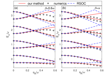
Figure 1: Energy levels $E_{n}/\omega$ obtained analytically (red solid line) as a function of effective coupling strength $\eta_{R}/\omega=\sqrt{2}\alpha/(l_{b}\omega)$ for different ration between the Dresselhaus and Rashba SOCs strength (a) $\beta/\alpha=0.6$ and (b) $\beta/\alpha=1$. The results obtained by the numerical exact diagonalization method (black circles) and under the RSOC approximation (blue dashed line) are listed for comparison. The parameters are $\Delta/\omega=0.5$, $l_{b}=1$ and $\omega=1$.

Fig. 1 displays the first eight energy levels as a function of the effective coupling strength $\eta_{R}/\omega=\sqrt{2}\alpha/(l_{b}\omega)$ for various values of the Dresselhaus coupling strength $\beta$. In the absence of the spin-orbit coupling $\eta_{R}=0$, one observes two separated $n$th Landau levels induced by the Zeeman energy $\Delta=0.5\omega$, in which the lower level is the spin-up state and the higher level corresponds to the spin-down electron state. As $\eta_{R}$ increases, the higher level of the $n$th Landau level state becomes lower due to the hybridization of the $n$th and $n+1$th displaced-Fock states induced by both types of SOCs. Comparing with the Rashba SOC approximation, the energy crossing occurs at a larger value of the coupling strength as a consequence of the Dresselhaus SOC. It demonstrates that the Dresselhaus SOC enhances Zeeman splitting, while the Rashba SOC interplay with the Zeeman splitting in opposite ways.

For the ratio between the Dresselhaus and Rashba SOC strengths $\beta/\alpha=0.6$, our analytical approach is in good agreement with the numerical results in a wide range of coupling strength $\eta_{R}/\omega<0.4$ in Fig. 1(a). There is noticeable deviation of the Rashba SOC results with the increasing of the coupling strength up to $\eta_{R}/\omega=0.3$. When the Dresselhaus and Rashba terms have equal strength with each other, $\beta=\alpha$, in Fig. 1(b), the deviation becomes more obvious. Because the Dresselhaus SOC play a more important effect as $\eta_{R}/\omega$ increases, and the Rashba SOC approximation fails. Therefore, our approach, which takes into account the effects of the Dresselhaus SOC terms, provides a more accurate analytical expression to the energy spectrum of the $2$DEG system.

IV Spin current with a electric field

Since the competition of the SOC and the Zeeman energy induces an energy crossing, the spin Hall resonance is closely related to the level crossing. When an external electric field is applied, the SOC of the $2$DEG induces the spin Hall effect, which is the transverse spin current response to the electric field. As the electric field $E$ is applied along the $y$ axis, the Hamiltonian becomes $H=H_{0}+eEy$ with the original Hamiltonian $H_{0}$ defined in Eq. (1). Using the replacement of $y$ by $y+eE/m\omega^{2}$ in the oscillator operator $a$, one obtains the quantized Hamiltonian

$$H=H_{0}+H_{E},H_{E}=-E[\frac{ke}{m\omega}+\frac{e}{\omega}(\alpha\sigma_{y}+\beta\sigma_{x})],$$ (29)

where $H_{0}$ is given in Eq.(1), and the constant $-e^{2}E^{2}/2m\omega^{2}$ is dropped. Similar to the transformed Hamiltonian $\tilde{H}_{0}$ in Eq. (21), we perform the unitary transformation $U=\exp[\sigma_{x}(a^{\dagger}\gamma-a\gamma^{\ast})]$ to $H_{E}$, resulting in

$$\tilde{H}_{E} = UH_{E}U^{{\dagger}}$$ (30)

$$= -E\frac{ke}{m\omega}-E\frac{\beta e}{\omega}\sigma_{x}-E\frac{\alpha e}{\omega}\{\sigma_{y}G(a^{\dagger}a)$$

$$+i\sigma_{z}[R(a^{\dagger}a)a^{\dagger}-aR(a^{\dagger}a)]\}.$$

The wave function for the Hamiltonian with the electric field can be given to the first-order correction in the perturbation in $\tilde{H}_{E}$ as

$$\left|\varphi_{\pm,n}^{(1)}\right\rangle=\left|\varphi_{\pm,n}\right\rangle+\sum_{n\neq k,l}\frac{\langle\varphi_{l,k}|\tilde{H}_{E}\left|\varphi_{\pm,n}\right\rangle}{E_{n,\pm}-E_{l,k}}\left|\varphi_{l,k}\right\rangle,(l=\pm),$$ (31)

where the eigenvalues $E_{n,\pm}$ and eigenstates $\left|\varphi_{\pm,n}\right\rangle$ are given in Eqs. (III)-(24).

The charge current operator of a single electron is given by

$$j_{c} = -e\upsilon_{x},$$ (32)

$$\upsilon_{x} = \frac{1}{i}[x,H]=\frac{p_{x}}{m}+\omega y+\alpha\sigma_{y}+\beta\sigma_{x},$$ (33)

and the spin-$z$ component current operator is

$$j_{s}^{z} = \frac{\hbar}{2}(S^{z}\upsilon_{x}+\upsilon_{x}S^{z})$$ (34)

$$= \frac{1}{2}[\sqrt{\frac{\omega}{2m}}(a^{{\dagger}}+a)-\frac{eE}{m\omega}]\sigma_{z}.$$

The average current density of the $N_{e}$ electron system is given by

$$I_{c(s)}=\frac{1}{L_{x}L_{y}}\sum_{nl}\langle j_{c(s)}\rangle_{nl}f(E_{nl}),(l=\pm 1),$$ (35)

where $f(E_{nl})$ is the Fermi distribution function, and $N_{e}=\sum_{nl}f(E_{nl})$. The charge Hall conductance is

$$G_{c(s)}=I_{c(s)}/E.$$ (36)

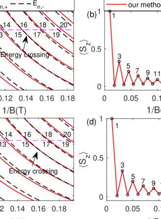
Figure 2: Energy levels $E_{n}$ and average spin $\langle S_{z}\rangle$ obtained analytically for an electron as a function of $1/B$ for $\beta=0$(a)(b) and $\beta/\alpha=0.5$ (c) (d) with $\Delta/\omega=0.5$ and $\alpha=0.25\omega$. The results of $\langle\sigma_{z}\rangle$ obtained by the numerical exact diagonalization (black circles) are listed for comparison.

Under the first-order perturbation, the corresponding spin/charge current can be expressed as $\langle j_{c(s)}\rangle_{\pm,n}=\langle j_{c(s)}^{(0)}\rangle_{\pm n}+\langle j_{c(s)}^{(1)}\rangle_{\pm n}$, where

$$\langle j_{c(s)}^{(0)}\rangle_{\pm n}=\left\langle\varphi_{\pm,n}\right|Uj_{c(s)}U^{{\dagger}}\left|\varphi_{\pm,n}\right\rangle,$$ (37)

$$\langle j_{c(s)}^{(1)}\rangle_{\pm n} = \sum\limits_{n\neq k,l}\frac{\left\langle\varphi_{\pm,n}\right|\tilde{H}_{E}\left|\varphi_{l,k}\right\rangle\left\langle\varphi_{l,k}\right|Uj_{c(s)}U^{{\dagger}}\left|\varphi_{\pm,n}\right\rangle}{E_{k,l}-E_{n,\pm}}$$ (38)

$$+h.c.$$

Under the zeroth approximation, one obtains analytical solutions

$$\left\langle j_{c}^{(0)}\right\rangle_{\pm n}=\frac{e^{2}E}{hN_{\phi}}L_{x}L_{y},\langle j_{s}^{z(0)}\rangle_{\pm,n}=-\frac{eE}{2m\omega}\left\langle\sigma_{z}\right\rangle_{\pm n},$$ (39)

where $\left\langle\sigma_{z}\right\rangle_{\pm n}$ is given in the Appendix B. With the average current density $I_{s}^{z}$, the spin Hall conductance can be derived under the zeroth order correction by

$$G_{s}^{z(0)}=-\frac{\langle S_{z}\rangle}{E}\frac{eE}{m\omega}=-\frac{\langle S_{z}\rangle G_{c}}{e},$$ (40)

$$\langle S_{z}\rangle=\sum_{nl}\frac{1}{2}\left\langle\sigma_{z}\right\rangle_{nl}f(E_{n,l}),(l=\pm).$$ (41)

And the Hall conductance is given as in the Appendix B

$$G_{c}=e^{2}N_{e}/(2\pi N_{\phi}),$$ (42)

which is only dependent on the filling factor $N_{e}/N_{\phi}$ with $N_{\phi}=L_{x}L_{y}eB/(hc)$ .

Fig. 2 shows energy levels and the spin polarization $\langle S_{z}\rangle$ under the zeroth approximation. It is observed that the energy $E_{n,+}$ with spin-up state firstly enters into the Fermi energy region, then it gives rise to the energy $E_{n+1,-}$ with spin-down state in Fig. 2(a)(c). As the energy gap between $E_{n,+}$ and $E_{n+1,-}$ becomes smaller, it yields energy crossing at certain magnetic field $B_{0}$, which is given by $E_{n+1,-}=E_{n,+}$ in Eq.(III). When the magnetic field exceeds the critical value $B_{0}$, the spin-down state with $E_{n,-}$ emerge firstly, and then the spin-up state with $E_{n+1,+}$ enters into the Fermi energy region. The corresponding expected value of $\langle S_{z}\rangle$ is calculated in Fig. 2(b)(d). It reaches maxima at odd integers $n$, and minima at even integers $n$. A discontinuous jump occurs at $B_{0}$. Below the critical value $B_{0}$, the maximal value of $\langle\sigma_{z}\rangle$ occurs at even integers $n$. The jump of the spin polarization ascribes to the energy crossing of two eigenstates with almost opposite spins. Especially, when only Rashba SOC is considered ($\beta=0$), one obtains the constraint condition for the energy crossing

$$2\omega=\sqrt{(\omega-\Delta)^{2}+4(n+1)\eta_{R}^{2}}+\sqrt{(\omega-\Delta)^{2}+4(n+2)\eta_{R}^{2}},$$ (43)

with the displacement $\gamma=0$ (see the Appendix C). It recovers results with only the Rashba coupling shen2004 . By comparing to the results with only Rashba SOC, the critical value of $1/B_{0}$ shifts to a larger value in Fig. 2(d). It demonstrates that the Dresselhaus SOC plays a vital role in suppressing the energy crossing, which is different from the effects of the Rashba SOC.

In presence of the electric field, the spin Hall conductance of the spin-$z$ component current is the most interesting. Fig. 3 shows the charge conductance $G_{c}$ in Eq. (42) and the spin Hall conductance $G_{s}^{z(1)}$ obtained by the first-order corrections in Eq. (38). A series of plateaus in the charge $G_{c}$ are visible, and a jump between two plateaus is observed at the critical magnetic field, where the spin conductance $G_{s}^{z(1)}$ becomes divergent with a resonant peak. The resonance ascribes to the interference of two degenerate levels near the Fermi energy. The resonance point coincides with the jump point of $\langle S_{z}\rangle$ with the energy crossing. By comparing to the behaviors with only the Rashba SOC, the charge $G_{c}$ and spin Hall conductance $G_{s}^{z(1)}$ exhibit a shift value of the resonant point, which is induced by the Dresselhaus SOC effects. For a large Zeeman splitting energy $\Delta/\omega=0.5$, the resonant point shifts to a larger value of $1/B_{0}$ in Fig. 3(b). It demonstrate that the SOC interactions and the Zeeman splitting play an opposite role in the energy-levels crossing. Fortunately, the charge and spin conductance obtained by first-order approximation agree well with the numerical results, exhibiting the validity of our approach.

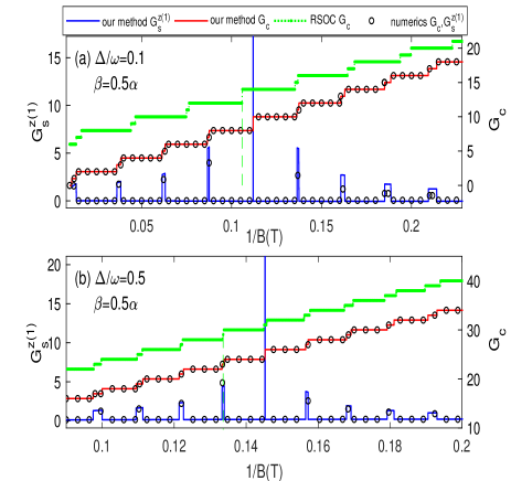
Figure 3: Charge conductance $G_{c}$ and spin Hall conductance $G_{s}^{z(1)}$ obtained with first-order corrections as a function of $1/B$ for different Zeeman splitting energy (a) $\Delta/\omega=0.1$ and (b) $\Delta/\omega=0.5$. The ratio between the Dresselhaus and Rashba SOCs is $\beta/\alpha=0.5$ with the Rashba SOC strength $\alpha=0.25\omega$. The results obtained by the numerical exact diagonalization (black circles) and under the RSOC approximation (blue dotted line) are listed for comparison. The external electronic field is $E/\omega=0.1N/C$.

V Conclusion

When both the Rashba and Dresselhaus spin-orbit couplings are considered, we find the single electron Hamiltonian in two-dimensional system subjected to a perpendicular magnetic field can map onto an anisotropic Rabi model. We perform the generalized Rashba SOC approximation using the displacement unitary transformation, and keep the single Landau level (nearest neighbor Landau level mixing) matrix element for even (odd) coupling function, and a solvable Hamiltonian is obtained in a similar form as that with only the Rashba term. The strengths of the both types of SOCs and Zeeman splitting are absorbed in the displacement-shift variable. With comparing the numerical diagonalization, our method provides accurate energy levels up to a large Zeeman splitting. As a consequence of the Dresselhaus and Rashba SOCs, each Landau state becomes a displaced-Fock state, which has a displacement shift by comparing to the original Harmonic oscillator Fock state. With the analytical solved eigenstates, the spin current displays a jump at a larger value of the inverse of the magnetic field, which demonstrates that the Dresselhaus SOC plays an opposite way in the energy splitting by comparing to the Rashba SOC. Moreover, in the presence of an electric field, the spin Hall conductance obtained by the first-order corrections diverges at the resonant point, and a series of plateaus of the charge conductance are observed, which fit well with numerical results. In conclusion, our method provides an easy-to-implement analytical solution to the 2DEGs with considering all SOCs in which all the coupling strengths, including Rashba, Dresselhaus, and Zeeman splitting, are described by the displacement shift. This solution could be potentially useful in the future studies of the quantum version of the spin Hall effects and the interacting fractional quantum Hall systems.

Appendix A Deviation of the Hamiltonian by the displacement transformation

We perform the unitrary transformation $U=\exp[\sigma_{x}(a^{\dagger}\gamma-a\gamma^{\ast})]$ to the Hamiltonian $H_{0}$ in Eq. (6). One easily obtains $UaU^{\dagger}=a-\gamma\sigma_{x}$ and $Ua^{\dagger}U^{\dagger}=a^{\dagger}-\gamma^{\ast}\sigma_{x}$. The first and second terms of $H_{0}$ in Eq. (6) can be transformed into

$$Ua^{\dagger}aU^{\dagger}=a^{\dagger}a-\sigma_{x}(a^{\dagger}\gamma+a\gamma^{\ast})+\gamma\gamma^{\ast},$$ (44)

and

$$U\sigma_{z}U^{\dagger}=\sigma_{z}\{1+\frac{1}{2}\sigma_{z}[2(a^{\dagger}\gamma-a\gamma^{\ast})]^{2}+...\}$$

$$-i\sigma_{y}\{2(a^{\dagger}\gamma-a\gamma^{\ast})+\frac{1}{3!}[2(a^{\dagger}\gamma-a\gamma^{\ast})]^{3}+...\}$$

$$= \sigma_{z}\cosh[2(a^{\dagger}\gamma-a\gamma^{\ast})]-i\sigma_{y}\sinh[2(a^{\dagger}\gamma-a\gamma^{\ast})].$$

Meanwhile, two SOCs terms of $H_{0}$ are derived explicitly as

$$U\sigma_{x}(a^{\dagger}e^{-i\theta}+ae^{i\theta})U^{\dagger}=\sigma_{x}(a^{\dagger}e^{-i\theta}+ae^{i\theta})-(\gamma^{\ast}e^{-i\theta}+\gamma e^{i\theta}),$$ (46)

and

$$Ui\sigma_{y}(a^{\dagger}e^{i\theta}-ae^{-i\theta})U^{\dagger}$$

$$=i\sigma_{y}B-\sigma_{z}[2AB-(\gamma e^{-i\theta}-\gamma^{\ast}e^{i\theta})]$$

$$+\frac{1}{2!}i\sigma_{y}[4A^{2}B-4A(\gamma e^{-i\theta}-\gamma^{\ast}e^{i\theta})]$$

$$-\frac{1}{3!}\sigma_{z}[8A^{3}B-12A^{2}(\gamma e^{-i\theta}-\gamma^{\ast}e^{i\theta})^{2}]$$

$$+\frac{1}{4!}i\sigma_{y}[16A^{4}B-32A^{3}(\gamma e^{-i\theta}-\gamma^{\ast}e^{i\theta})]+...$$

$$= i\sigma_{y}[\cosh(2A)B-(\gamma e^{-i\theta}-\gamma^{\ast}e^{i\theta})\sinh(2A)]$$

$$-\sigma_{z}[\sinh(2A)B-(\gamma e^{-i\theta}-\gamma^{\ast}e^{i\theta})\cosh(2A)]$$

where the operators are given by $A=a^{\dagger}\gamma-a\gamma^{\ast}$ and $B=a^{\dagger}e^{i\theta}-ae^{-i\theta}$. Thus, the transformed Hamiltonian is given in terms of $H_{0}^{\prime}$ and $H_{1}^{\prime}$ in Eqs. (17) and (8).

By expanding the even and odd functions $\cosh[2(a^{\dagger}\gamma-a\gamma^{\ast})]$ and $\sinh[2(a^{\dagger}\gamma-a\gamma^{\ast})]$, the corresponding coefficients are derived as

$$G_{n,n} = \left\langle n\right|\cosh[2(a^{\dagger}\gamma-a\gamma^{\ast})]\left|n\right\rangle$$ (47)

$$= \frac{1}{2}\left\langle n\right|\{\exp[2(a^{\dagger}\gamma-a\gamma^{\ast})]+\exp[-2(a^{\dagger}\gamma-a\gamma^{\ast})]\}\left|n\right\rangle$$

$$= e^{-2\gamma\gamma^{\ast}}\sum_{i=0}^{n}(-1)^{n-i}\frac{n!}{(n-i)!(n-i!)i!}(4\gamma\gamma^{\ast})^{n-i}$$

$$= e^{-2\gamma\gamma^{\ast}}L_{n}(4\gamma\gamma^{\ast}),$$

and

$$\sqrt{n+1}R_{n+1,n}=\left\langle n+1\right|\sinh[2(a^{\dagger}\gamma-a\gamma^{\ast})]\left|n\right\rangle$$ (48)

$$= \frac{1}{2}\left\langle n\right|\{\exp[2(a^{\dagger}\gamma-a\gamma^{\ast})]-\exp[-2(a^{\dagger}\gamma-a\gamma^{\ast})]\}\left|n\right\rangle$$

$$= \frac{2\gamma e^{-2\gamma\gamma^{\ast}}}{\sqrt{n!(n+1)!}}\sum_{i=0}^{n}(-1)^{n-i}\frac{n!(n+1)!}{(n-i)!(n+1-i!)i!}(4\gamma\gamma^{\ast})^{n-i}$$

$$= \frac{2\gamma}{\sqrt{n+1}}e^{-2\gamma\gamma^{\ast}}L_{n}^{1}(4\gamma\gamma^{\ast}).$$

Appendix B Spin current under the zeroth corrections

In presence of the electric field, the spin current is derived as

$$\left\langle j_{s}^{z}\right\rangle_{\pm n}=\frac{1}{2}\langle\varphi_{\pm,n}|U[\sqrt{\frac{\hbar\omega}{2m}}(a^{{\dagger}}+a)-\frac{eE}{m\omega}]\sigma_{z}U^{\dagger}\left|\varphi_{\pm,n}\right\rangle.$$

Using the eigenstates $\left|\varphi_{\pm,n}\right\rangle$ in Eqs. (23) and (24), one obtains

$$\langle(a^{{\dagger}}+a)\sigma_{z}\rangle_{+n}=\left\langle\varphi_{+,n}\right|U(a^{{\dagger}}+a)\sigma_{z}U^{{\dagger}}\left|\varphi_{+,n}\right\rangle$$ (50)

$$= \left\langle\varphi_{+,n}\right|[(a^{{\dagger}}+a)-(\gamma+\gamma^{\ast})\sigma_{x}]U\sigma_{z}U^{\dagger}\left|\varphi_{+,n}\right\rangle$$

$$= \left\langle n\right|(a^{\dagger}+a)\sinh[2(a^{\dagger}\gamma-a\gamma^{\ast})]\sin^{\ast}\frac{\theta_{n}}{2}\cos\frac{\theta_{n}}{2}\left|n+1\right\rangle$$

$$-\left\langle n+1\right|(a^{\dagger}+a)\sinh[2(a^{\dagger}\gamma-a\gamma^{\ast})]\cos^{\ast}\frac{\theta_{n}}{2}\sin\frac{\theta_{n}}{2}\left|n\right\rangle$$

$$= 0,$$

and

$$\langle(a^{{\dagger}}+a)\sigma_{z}\rangle_{-n}=\left\langle\varphi_{-,n}\right|U(a^{{\dagger}}+a)\sigma_{z}U^{{\dagger}}\left|\varphi_{-,n}\right\rangle=0.$$ (51)

So the spin current is simplified as

$$\left\langle j_{s}^{z}\right\rangle_{\pm n}=-\frac{eE}{2m\omega}\left\langle\sigma_{z}\right\rangle_{\pm n}.$$ (52)

where the average value of $\left\langle\sigma_{z}\right\rangle_{\pm n}$ are derived in the following

$$\left\langle\sigma_{z}\right\rangle_{+n}=\langle\varphi_{+,n}|U\sigma_{z}U^{\dagger}\left|\varphi_{+,n}\right\rangle$$

$$=\cos\frac{\theta_{n}}{2}\cos^{\ast}\frac{\theta_{n}}{2}G_{n+1,n+1}-\sin\frac{\theta_{n}}{2}\sin^{\ast}\frac{\theta_{n}}{2}G_{n,n}$$

$$-\sqrt{n+1}(\sin\frac{\theta_{n}}{2}\cos^{\ast}\frac{\theta_{n}}{2}R_{n+1,n}+\sin^{{}^{\ast}}\frac{\theta_{n}}{2}\cos\frac{\theta_{n}}{2}R_{n,n+1}),$$

and

$$\left\langle\sigma_{z}\right\rangle_{-n}=\langle\varphi_{-,n}|U\sigma_{z}U^{\dagger}\left|\varphi_{-,n}\right\rangle$$

$$=\sin\frac{\theta_{n}}{2}\sin^{\ast}\frac{\theta_{n}}{2}G_{n+1,n+1}-\cos\frac{\theta_{n}}{2}\cos^{\ast}\frac{\theta_{n}}{2}G_{n,n}$$

$$+\sqrt{n+1}(\cos\frac{\theta_{n}}{2}\sin^{\ast}\frac{\theta_{n}}{2}R_{n+1,n}+\cos^{\ast}\frac{\theta_{n}}{2}\sin\frac{\theta_{n}}{2}R_{n,n+1}).$$

Meanwhile, the charge current $j_{c}=-ev_{x}$ can be expressed in terms of the harmonic oscillator $a$ ($a^{\dagger}$) as

$$j_{c}=-e[\sqrt{\frac{\hbar\omega}{2m}}(a^{\dagger}+a)+\alpha\sigma_{y}+\beta\sigma_{x}-\frac{eE}{m\omega}].$$ (55)

The average value of the charge current is given by

$$\left\langle j_{c}\right\rangle_{\pm n} = \langle\varphi_{\pm,n}|Uj_{c}U^{{\dagger}}\left|\varphi_{\pm,n}\right\rangle$$ (56)

$$= \left\langle\varphi_{\pm,n}\right|\frac{e^{2}E}{m\omega}\left|\varphi_{\pm,n}\right\rangle=\frac{e^{2}E}{2\pi N_{\phi}}L_{x}L_{y},$$

where $Uj_{c}U^{{\dagger}}=-e[\sqrt{\frac{\omega}{2m}}(a^{\dagger}+a)-\sqrt{\frac{\omega}{2m}}(\gamma+\gamma^{\ast})\sigma_{x}+\alpha\sigma_{y}\cosh(2A)+\alpha i\sigma_{z}\sinh(2A)+\beta\sigma_{x}-eE/(m\omega)]$. Then we obtain the charge Hall conductance $G_{c}=I_{c}/E$ as

$$G_{c}=\frac{e^{2}E}{2\pi EN_{\phi}}\sum_{nl}f(E_{nl})=\frac{e^{2}N_{e}}{2\pi N_{\phi}}.$$ (57)

Appendix C energy-crossing conditions

Since the $n+1$-th Laudau level of spin down and the $n$-th Laudau level of spin-up becomes crossing near the Fermi energy, resulting in the resonance peak of the spin Hall conductance at the energy crossing point. It leads to the energy crossing at certain magnetic field $B_{0}$, which satisfies $E_{n+1,-}=E_{n,+}$. It yields

$$2\omega+f(n+2)-2f(n+1)+f(n)$$

$$=\sqrt{[f(n+1)+f(n)+\omega]^{2}+4(n+1)|\widetilde{\alpha}_{n,n+1}|^{2}}$$

$$+\sqrt{[f(n+2)+f(n+1)+\omega]^{2}+4(n+2)|\widetilde{\alpha}_{n+1,n+2}|^{2}}.$$

Especially, when the Dresshaul SOC is neglected by setting $\beta=0$, the displacement variable reduces into $\gamma=0$. One can simplify the parameters as $R_{n,n+1}=R_{n+1,n}=0$, $T_{n,n+1}=-i\alpha/\sqrt{\alpha^{2}+\beta^{2}}$, $\eta_{0}=\omega/2$, $\eta_{1}=-\Delta/2$, $f(n)=-\Delta/2$, and $\widetilde{\alpha}_{n,n+1}=i\eta_{R\text{ }}$. It leads to the eigenvalues

$$E_{n,+}=\omega n+\omega+\frac{1}{2}\sqrt{(\omega-\Delta)^{2}+4(n+1)\eta_{R}^{2}},$$ (59)

$$E_{n+1,-}=\omega(n+1)+\omega-\frac{1}{2}\sqrt{(\omega-\Delta)^{2}+4(n+2)\eta_{R}^{2}}.$$ (60)

Thus, the energy-levels crossing is given by $E_{n+1,-}-E_{n,+}=0$, resulting in

$$2\omega=\sqrt{(\omega-\Delta)^{2}+4(n+1)\eta_{R}^{2}}+\sqrt{(\omega-\Delta)^{2}+4(n+2)\eta_{R}^{2}}.$$ (61)

References

- (1) J. Fabian, A. Matos-Abiague, C. Ertler, P. Stano and I. Zutic, Acta Phys. Slovaca 57, 565 (2007).
- (2) C. Chappert, A. Fert and F. N. Van Dau, Nature Mater. 6, 813 (2007).
- (3) M. I. Dyakonov and V. I. Peral, ZhETF Pis. Red. 13, 657 (1971).
- (4) J. Hirsch, Phys. Rev. Lett. 83, 1834 (1999).
- (5) S. Murakami, N. Nagaosa, and S. C. Zhang, Science 301, 1348 (2003).
- (6) J. Sinova, D. Culcer, Q. Niu, N. A. Sinitsyn, T. Jungwirth, and A. H. MacDonald, Phys. Rev. Lett. 92, 126603 (2004).
- (7) D. Xiao, M-C. Chang, and Q. Niu, Rev. Mod. Phys. 82, 1959 (2010).
- (8) Y. K. Kato, R. C. Myers, A. C. Gossard, and D. D. Awschalom, Science 306, 1910(2004).
- (9) J. Wunderlich, B. Kaestner, J. Sinova and T. Jungwirth, Phys. Rev. Lett. 94, 047204 (2005).
- (10) J. Wunderlich, et al, Science 330, 1801 (2010).
- (11) S. O. Valenzuela and M. Tinkham, Nature 442, 176 (2006).
- (12) J. Sinova, S. O. Valenzuela, J. Wunderlich, C.H. Back, and T. Jungwirth, Rev. Mod. Phys. 87, 1213 (2015).
- (13) S. Q. Shen, M. Ma, X. C. Xie, and F. C. Zhang, Phys. Rev. Lett. 92, 256603 (2004).
- (14) P. Lucignano, R. Raimondi, and A. Tagliacozzo, Phys. Rev. B 78, 035336 (2008).
- (15) H. A. Engel, E. I. Rashba, and B. I. Halperin, Phys. Rev. Lett. 98, 036602 (2007).
- (16) E. Rashba, Sov. Phys. Solid State 2, 1109 (1960).
- (17) G. Dresselhaus, Phys. Rev. 100, 580 (1955).
- (18) Y. A. Bychkov, E. Rashba, J. Phys. C: Solid State Phys. 17, 6039 (1984).
- (19) B. Jusserand, D. Richards, H. Peric, and B. Etienne, Phys. Rev. Lett. 69, 848 (1992).
- (20) M. Kim, J. Ihm, and S. B. Chung, Phys. Rev. B 94, 115431 (2016).
- (21) K. Ishizaka, et al., Nat. Mater 10, 521 (2011)
- (22) A. Manchon, H. C. Koo, J. Nitta, S. M. Frolov, and R. A. Duine, Nat. Mater. 14, 871 (2015).
- (23) G. Lommer, F. Malcher, and U. Rössler, Phys. Rev. Lett. 60, 728 (1988).
- (24) O. Voskoboynikov, C. P. Lee, and O. Tretyak, Phys. Rev. B 63, 165306 (2001).
- (25) J. Schliemann, and D. Loss, Phys. Rev. B 68, 165311 (2003).
- (26) S. D. Ganichev, V. V. Bel?kov, L. E. Golub, E. L. Ivchenko, Petra Schneider, S. Giglberger, J. Eroms, J. De Boeck, G. Borghs, W. Wegscheider, D. Weiss, and W. Prettl, Phys. Rev. Lett. 92, 256601 (2004).
- (27) N. S. Averkiev, L. E. Golub, Phys. Rev. B 60, 15582 (1999).
- (28) H. K. Park, H. J. Yang, and S. Lee, Phys. Rev. Res. 2, 033487 (2020).
- (29) S. Gelfert, C. Frankerl, C. Reichl, D. Schuh, G. Salis, W. Wegscheider, D. Bougeard, T. Korn, and C. Schüller, Phys. Rev. B 101, 035427 (2020).
- (30) Y. Ohno, R. Terauchi, T. Adachi, F. Matsukura, and H. Ohno, Phys. Rev. Lett. 83, 4196 (1999).
- (31) O. Z. Karimov, G. H. John, R.T. Harley, W. H. Lau, M. E. Flatte, M. Henini, and R. Airey, Phys. Rev. Lett. 91, 246601 (2003).
- (32) S. Döhrmann, D. Hägele, J. Rudolph, M. Bichler, D. Schuh, and M. Oestreich, and M. Oestreich, Phys. Rev. Lett. 93, 147405 (2004).
- (33) V. V. Bel?kov, P. Olbrich, S. A. Tarasenko, D. Schuh, W. Wegscheider, T. Korn, C. Schüller, D. Weiss, W. Prettl, and S. D. Ganichev, Phys. Rev. Lett. 100, 176806 (2008).
- (34) G. M. Müller, M. Römer, D. Schuh, W. Wegscheider, J. Hübner, and M. Oestreich, Phys. Rev. Lett. 101, 206601 (2008).
- (35) A. Balocchi, Q. H. Duong, P. Renucci, B. L. Liu, C. Fontaine, T. Amand, D. Lagarde, and X. Marie, Phys. Rev. Lett. 107, 136604 (2011).
- (36) A. Hernández-Mínguez, K. Biermann, R. Hey, and P. V. Santos, Phys. Rev. Lett. 109, 266602 (2012).
- (37) J. Nitta, T. Akazaki, H. Takayanagi, and T. Enoki, Phys. Rev. Lett. 78, 1335 (1997).
- (38) J. P. Heida, B. J. van Wees, J. J. Kuipers, T. M. Klapwijk, and G. Borghs, Phys. Rev. B 57, 11911 (1998).
- (39) S. Q. Shen, Y. J. Bao, M. Ma, X. C. Xie, and F. C. Zhang, Phys. Rev. B 71, 155316 (2005).
- (40) W. Yang, and K. Chang, Phys. Rev. B 73, 045303 (2006).
- (41) R. Li, J. Q. You, C. P. Sun, and F. Nori, Phys. Rev. Lett. 111, 086805 (2013).
- (42) Q. H. Chen, C. Wang, S. He, T. Liu, and K. L. Wang, Phys. Rev. A 86, 023822 (2012).
- (43) E. K. Irish, Phys. Rev. Lett. 99, 173601(2007).
- (44) Y. Y. Zhang Phys. Rev. A 94, 063824 (2016); Y. Y. Zhang and X.Y. Chen, Phys. Rev. A 96, 063821 (2017).