A New Weighting Scheme for Fan-beam and Circle Cone-beam CT Reconstructions

Abstract

In this paper, we first present an arc based algorithm for fan-beam computed tomography (CT) reconstruction via applying Katsevich’s helical CT formula to 2D fan-beam CT reconstruction. Then, we propose a new weighting function to deal with the redundant projection data. By extending the weighted arc based fan-beam algorithm to circle cone-beam geometry, we also obtain a new FDK-similar algorithm for circle cone-beam CT reconstruction. Experiments show that our methods can obtain higher PSNR and SSIM compared to the Parker-weighted conventional fan-beam algorithm and the FDK algorithm for super-short-scan trajectories.

I Introduction

Computed tomography (CT) has been widely used in clinical diagnosis and industrial applications since its ability of providing inner vision of an object without destructing it. In classical tomography, the fan-beam CT reconstruction algorithm is fundamental since it can be heuristically extended to 3D helical cone-beam [1][2][3][4][5][6] and circle cone-beam [7][8][9][10][11][12] CT reconstructions. The standard fan-beam reconstruction method is the ramp filter-based filtered backprojection (FBP) algorithm [13][14], which can be derived from the Radon inversion formula. For 2D CT image reconstruction, to exactly and stably reconstruct the whole image, it requires to measure all the line integrals of the X-rays that diverge from all directions and pass through the object. To make a fan-beam CT that samples data on a circular trajectory meet this condition, the detector must be large enough to cover the fan-angle of $\pm\gamma_{m}=\arcsin(R_{m}/R_{o})$ to avoid truncated projections and the X-ray source must travel on a continuous arc of $\pi+2\gamma_{m}$ on the circle to ensure that the line integrals of the X-rays diverging from all directions in the 2D plane and passing through the object are measured, where $R_{o}$ is the radius of the scanning trajectory and $R_{m}<R_{o}$ is the radius of the object. In the literature, the range of $\pi+2\gamma_{m}$ is called as short-scan. In [15], Parker proposed a weighting function to weight the short-scan fan-beam projection data before convoluting it to avoid completing the projection data of the remain angles ([$\pi+2\gamma_{m}$:$2\pi$]) and implement the reconstruction algorithm efficiently. When the range of scanning angles is larger than the short-scan, redundant projection data is measured. In [16], Silver extended Parker’s weighting function by utilizing the virtual detectors to tackle these redundant projection data.

In 2002, Noo et al. [17] proposed another type of FBP algorithm for fan-beam CT reconstruction by decomposing the convolution of the ramp filter into a successive convolutions of a Hilbert filter and a derivative filter. After that, many other algorithms [9][18][19] based on the Hilbert transform were proposed. One advantage of these new algorithms is that they can exactly reconstruct a part of the image even though the range of the scanning angles is less than the short scan. These new algorithms can be seen as special cases that applying the 3D exact helical cone-beam inversion formula [20][21] to the 2D CT reconstructions. In [22], You et al. derived a Hilbert transform based FBP algorithm for fan-beam full- and partial-scans, in which the backprojection does not include position-dependent weights. In [9] and [17], to deal with the redundant data, a continuous weight function was also proposed to weight the filtered sinograms.

A specific view-dependent data differentiation was a common processing step in these Hilbert transform based algorithms. In [3][23], the implementation of this step was researched in order to improve the resolution and quality of the reconstructed image. In [4], Zamyatin et al. used the Taylor series expansions to approximate the derivative of the Hilbert transform and proposed new algorithms for fan-beam and helical cone-beam CT reconstruction.

The fan-beam algorithms can be heuristically extended to 3D cone-beam CT reconstructions [1][2][3][5][6] [7][9][11][12][24], which are referred to as approximating algorithms. On the other hand, there exist a lot of exact cone-beam algorithms [10][20][21][25][26][27] in the literature. The advantages of the approximating algorithms are that they are easy to implement and flexible to modulate the ramp kernel for different clinical applications, while those of the exact algorithms are that they can reconstruct images with good resolution even when the cone angle is large. In [2][6][10][11][12][24][27], the weighting functions are also proposed to tackle the redundant cone-beam projection data.

In this paper, we first present an arc based algorithm for fan-beam CT reconstruction by applying Katsevich’s helical CT [17] formula to 2D fan-beam CT reconstruction. Then, we propose a new weighting function to tackle the redundant projection data. By extending the arc based algorithm to the circle cone-beam geometry, we also obtain a new algorithm for circle cone-beam CT reconstruction. Our weighting function is different from the ones used in [9][15][17]. The weighting functions in [9][15][17] depend on the rotation angle of the X-ray source and the diverging direction of the X-ray, and are required to be continuous with respect to these arguments while our weighting function depends on the rotation angle of the X-ray source and the positions of the pixels of the reconstructed image, and has no continuity constraint. Thus, the CT images reconstructed by our method may have higher resolutions and less artifacts. Moreover, there exists a hyper-parameter in the weighting functions of [9] [17] that greatly influences the performance of the algorithm while our weighting function has no hyper-parameter.

The rest of the paper is organized as follows. In Section II we briefly introduce the related works. In Section III, we present an arc based algorithm for fan-beam CT reconstruction and derive a weighting function for tackling the redundant data, and then extend the algorithm with the weighting function to circular cone-beam CT reconstruction. Numerical evaluation is presented in Section IV, followed by conclusion in Section V.

II Related works

In this section, we briefly describe some works related to our method.

II-A Noo’s fan-beam formula

In [17], Noo et al. decomposed the convolution of the ramp filter into a successive convolutions of the Hilbert filter and the derivative filter in the Fourier domain by observing that

$$|\sigma|=(1/2\pi)(i2\pi\sigma)(-i\text{sign}(\sigma)),$$ (1)

where $|\sigma|$, $i2\pi\sigma$ and $-i\text{sign}(\sigma)$ are the Fourier transform of the ramp filter, the derivative filter and the Hilbert filter, respectively. By utilizing this relationship, they proposed a FBP reconstruction formula for fan-beam CT.

Let

$$g(\lambda,\gamma)=g(\lambda,\underline{a}(\gamma))$$ (2)

be the measured projections, where $\lambda$ is a polar angle of the X-ray source, $\underline{a}(\lambda)=\left(R_{o}\cos\lambda,R_{o}\sin\lambda\right)$ is a position of the X-ray source, $R_{o}$ is the radius of the trajectory circle of the X-ray source, $\underline{\gamma}=\cos\gamma\underline{e}_{1}+\sin\gamma\underline{e}_{2}$ is a diverging direction of the X-ray, $\gamma\in\left[-\gamma_{m},\gamma_{m}\right]$, $\gamma_{m}$ is the half fan-angle, $\underline{e}_{1}=-(\cos\lambda,\sin\lambda)$, and $\underline{e}_{2}=(-\sin\lambda,\cos\lambda)$. Then the reconstruction formula for fan-beam CT with equi-angular detetcor reads:

$$f(\underline{x})=\frac{1}{2\pi}\int_{\Lambda}\mathrm{d}\lambda\frac{1}{\|\underline{x}-\underline{a}(\lambda)\|}\left[w(\lambda,\phi)g_{F}(\lambda,\phi)\right]_{\phi=\phi^{*}(\lambda,\underline{x})},$$ (3)

where $\Lambda$ is the X-ray source trajectory satisfying the data completeness condition [17],

$$\phi^{*}(\lambda,\underline{x})=\arctan\frac{x\cdot\underline{e}_{2}}{R_{o}+\underline{x}\cdot\underline{e}_{1}},\quad\left|\phi^{*}(\lambda,\underline{x})\right|<\pi/2$$ (4)

is the angle characterizing the ray that diverges from $\underline{a}(\lambda)$ and passes $\underline{x}$,

$$g_{F}(\lambda,\phi)=\int_{-\gamma_{m}}^{\gamma_{m}}\text{d}\gamma h_{H}(\sin(\phi-\gamma))\left(\frac{\partial}{\partial\lambda}+\frac{\partial}{\partial\gamma}\right)g(\lambda,\gamma),$$ (5)

$$h_{H}(s)=-\int_{-\infty}^{+\infty}\mathrm{d}\sigma\mathrm{i}\operatorname{sgn}(\sigma)\mathrm{e}^{\mathrm{i}2\pi\sigma s}=\frac{1}{\pi s}$$ (6)

is the Hilbert filter and

$$w(\lambda,\phi)=\frac{c(\lambda)}{c(\lambda)+c(\lambda+\pi-2\phi)}$$ (7)

is the weighting function with

$$c(\lambda)=\left\{\begin{array}[]{ll}\cos^{2}\frac{\pi\left(\lambda-\lambda_{s}-d\right)}{2d}&\text{ if }\quad\lambda_{s}<\lambda<\lambda_{s}+d,\\ 1&\text{ if }\quad\lambda_{s}+d<\lambda<\lambda_{e}-d,\\ \cos^{2}\frac{\pi\left(\lambda-\lambda_{e}+d\right)}{2d}&\text{ if }\quad\lambda_{e}-d<\lambda<\lambda_{e}\end{array}\right.$$ (8)

and $d$ is an angular interval over which $c(\lambda)$ smoothly drops from 1 to 0. In the experiments, they set $d=10\pi/180$.

Applying the changes of variables $u=D\tan\gamma$ and $\tilde{u}=D\tan\phi$ in equations (3) and (5), they obtain the reconstruction formula for fan-beam CT with equally spaced collinear detectors:

$$f(\underline{x})=\frac{1}{2\pi}\int_{\Lambda}\mathrm{d}\lambda\frac{1}{R_{o}+\underline{x}\cdot e_{1}}\left[w(\lambda,\tilde{u})g_{F}(\lambda,\tilde{u})\right]_{\tilde{u}=\tilde{a}^{*}(\lambda,\underline{x})}$$ (9)

with

$$g_{F}(\lambda,\tilde{u})=\int_{-u_{m}}^{u_{m}}\text{d} uh_{H}(\tilde{u}-u)\frac{D}{\sqrt{D^{2}+u^{2}}}$$ (10)

$$\left(\frac{\partial}{\partial\lambda}+\frac{D^{2}+u^{2}}{D}\frac{\partial}{\partial u}\right)g(\lambda,u),$$

where $u_{m}=D\tan\gamma_{m}$,

$$\tilde{u}^{*}(\lambda,\underline{x})=D\tan\phi^{*}(\lambda,\underline{x})=\frac{D\underline{x}\cdot\underline{e}_{2}}{R_{o}+\underline{x}\cdot\underline{e}_{1}}$$ (11)

is the detector location of the line connecting $\underline{x}$ to $\underline{a}(\lambda)$ and

$$w(\lambda,\tilde{u})=\frac{c(\lambda)}{c(\lambda)+c(\lambda+\pi-2\arctan(\tilde{u}/D))}.$$ (12)

II-B Katsevich’s helical cone-beam formula

In [21], Katsevich proposed an exact reconstruction formula for helical cone-beam CT and Noo et al. [28] researched how to efficiently and accurately implement it. The reconstruction formula can be written as

$$f(\underline{x})=-\frac{1}{2\pi}\int_{\lambda_{i}(\underline{x})}^{\lambda_{o}(\underline{x})}\mathrm{d}\lambda\frac{1}{\|\underline{x}-\underline{a}(\lambda)\|}g^{F}\left(\lambda,\frac{\underline{x}-\underline{a}(\lambda)}{\|\underline{x}-\underline{a}(\lambda)\|}\right)$$ (13)

where $\lambda_{i}(x)$ and $\lambda_{o}(x)$ are the extremities of the $\pi$-line passing through $x$ with $\lambda_{i}(x)<\lambda_{o}(x)$,

$$g^{F}(\lambda,\underline{\theta})=\int_{0}^{2\pi}\mathrm{d}\gamma h_{H}(\sin\gamma)g^{\prime}(\lambda,\cos\gamma\underline{\theta}+\sin\gamma(\underline{\theta}\times\underline{m}(\lambda,\underline{\theta}))),$$ (14)

$$g^{\prime}(\lambda,\underline{\theta})=\lim_{\varepsilon\rightarrow 0}\frac{g(\lambda+\varepsilon,\underline{\theta})-g(\lambda,\underline{\theta})}{\varepsilon},$$ (15)

$h_{H}(s)$ is the Hilbert filter defined in equation (6), $g(\lambda,\underline{\theta})$ is the measured projection data and vector $\underline{m}(\lambda,\underline{\theta})$ is normal to the $\kappa$-plane $\mathcal{K}(\lambda,\psi)$ of the smallest $|\psi|$ value that contains the line of direction $\underline{\theta}$ through $\underline{a}(\lambda)$.

III Proposed Method

III-A Arc based fan-beam algorithm

Applying equation (13) to the 2D fan-beam reconstruction, the $\pi$-line becomes a chord of the circle of the scanning trajectory, the $\kappa$-plane $\mathcal{K}(\lambda,\psi)$ coincides with the image plane to reconstruct and so $\underline{\theta}\times\underline{m}(\lambda,\underline{\theta})=\underline{\theta}^{\bot}$.

Let $\underline{a}(\lambda)=\left(R_{o}\cos\lambda,R_{o}\sin\lambda\right)$ be the position of the X-ray source on the trajectory circle of radius $R_{o}$ and

$$g(\lambda,\underline{\theta})=\int_{0}^{+\infty}\mathrm{d}tf(\underline{a}(\lambda)+t\underline{\theta})$$ (16)

be the measured projection data, where $\underline{\theta}\in S^{1}$ is a diverging direction of the X-ray and $S^{1}$ is the unit circle in the 2D plane. Then, according to equation (13), the reconstruction formula for fan-beam CT can be written as

$$f(\underline{x})=-\frac{1}{2\pi}\int_{\text{chord}(\underline{x})}\mathrm{d}\lambda\frac{1}{\|\underline{x}-\underline{a}(\lambda)\|}g^{F}\left(\lambda,\frac{\underline{x}-\underline{a}(\lambda)}{\|\underline{x}-\underline{a}(\lambda)\|}\right),$$ (17)

where $|\underline{x}|<R_{m}<R_{o}$, $R_{m}$ is the radius of the test object,

$$g^{F}(\lambda,\underline{\theta})=\int_{0}^{2\pi}\mathrm{d}\bar{\gamma}h_{H}(\sin\bar{\gamma})g^{\prime}(\lambda,\cos\bar{\gamma}\underline{\theta}+\sin\bar{\gamma}\underline{\theta}^{\bot}),$$ (18)

$h_{H}(s)$ and $g^{\prime}(\lambda,\underline{\theta})$ are defined by equations (6) and (15), respectively, $\text{chord}(\underline{x})$ is a chord passing through $\underline{x}$ and dividing the trajectory circle into two arcs, and the integral $\text{d}\lambda$ is done on any one of the two arcs.

Figure 1: An example of the X-ray source trajectory. The projection data measured along the three red arcs can be used to reconstruct the intensity of $\underline{x}$.

From equation (17), we can argue that the intensity of any point $\underline{x}$ with $|\underline{x}|<R_{m}<R_{o}$ in the circle can be reconstructed if there exists a chord passing through $\underline{x}$ such that all the projections $g(\lambda,\underline{\theta})$ on the corresponding arcs of the chord passing through the neighborhood of $\underline{x}$ are measured. Note that $g(\lambda,\underline{\theta})$ can be measured from another direction since $g(\lambda,\underline{\theta})=g(\lambda_{1},-\underline{\theta})$, where $\underline{\theta}=\frac{\underline{a}(\lambda_{1})-\underline{a}(\lambda)}{|\underline{a}(\lambda_{1})-\underline{a}(\lambda)|}$. See Fig. 1 for example.

For any fixed $\underline{x}$ in the trajectory circle, there may exist many available chords passing through $\underline{x}$ and so the integral arcs can be different. Moreover, when the range of scanning arc is larger than the short scan, redundant projection data needs to be processed. A simple method to tackle these redundant projection data is to calculate equation (17) for all available chords and average them. However, averaging them is equivalent to filtering the reconstructed image by a low-pass filter and so may reduce the resolution of the reconstructed image. In this paper we only consider two types of chords that respectively pass through the two endpoints of the scanning arcs.

Therefore, we propose the following formula for fan-beam reconstruction:

$$f(\underline{x})=-\frac{1}{2\pi}\int_{\lambda_{0}}^{\lambda_{P}}\mathrm{d}\lambda\frac{\varpi(\underline{x},\lambda)}{\|\underline{x}-\underline{a}(\lambda)\|}g^{F}\left(\lambda,\frac{\underline{x}-\underline{a}(\lambda)}{\|\underline{x}-\underline{a}(\lambda)\|}\right),$$ (19)

where $\lambda_{0}<\lambda_{P}$ correspond to the two endpoints of the scanning arcs,

$$\varpi(\underline{x},\lambda)=\frac{1}{2}(\varpi_{1}(\underline{x},\lambda)+\varpi_{2}(\underline{x},\lambda))$$ (20)

is a weighting function, and $\varpi_{1}(\underline{x},\lambda)$ and $\varpi_{2}(\underline{x},\lambda)$ are defined by

$$\varpi_{1}(\underline{x},\lambda)=\left\{\begin{array}[]{l}1,~{}~{}~{}~{}~{}~{}\text{if}~{}~{}\underline{a}(\lambda)\in\wideparen{\underline{a}(\lambda_{0}),\underline{a}(\lambda(\underline{x},\lambda_{0}))},\\ 0~{}~{}~{}~{}~{}~{}~{}\text{else},\end{array}\right.$$ (21)

$$\varpi_{2}(\underline{x},\lambda)=\left\{\begin{array}[]{l}1,~{}~{}~{}~{}~{}~{}\text{if}~{}~{}\underline{a}(\lambda)\in\wideparen{\underline{a}(\lambda(\underline{x},\lambda_{P})),\underline{a}(\lambda_{P})},\\ 0~{}~{}~{}~{}~{}~{}~{}\text{else},\end{array}\right.$$ (22)

where $\underline{a}(\lambda(\underline{x},\lambda_{0}))$ is another endpoint of the chord passing through $\underline{a}(\lambda_{0})$ and $x$, $\underline{a}(\lambda(\underline{x},\lambda_{P}))$ is another endpoint of the chord passing through $\underline{a}(\lambda_{P})$ and $x$, and $\wideparen{\underline{a}(\lambda_{0}),\underline{a}(\lambda(\underline{x},\lambda_{0}))}$ denotes the arc starting from $\underline{a}(\lambda_{0})$ and ending at $\underline{a}(\lambda(\underline{x},\lambda_{0}))$.

III-A1 Implementation for the curved-line detector

In this subsection, we describe how to implement equation (19) when the fan-beam projections are measured by using an equi-angular curved-line detector.

Figure 2: Geometry of data acquisition by using an equi-angular curved detector.

Let $\underline{a}(\lambda)=\left(R_{o}\cos\lambda,R_{o}\sin\lambda\right)$ be the position of the X-ray source, $\underline{\theta}(\lambda,\gamma)=\cos\gamma\underline{e}_{0}(\lambda)+\sin\gamma\underline{e}_{1}(\lambda)$ be the diverging direction, $g_{c}(\lambda,\gamma)=g(\lambda,\underline{\theta}(\lambda,\gamma))$ be the measured projection data using the curved-line detector, where $\gamma$ is the sampling coordinate of the fan-angle, $\underline{e}_{0}(\lambda)=(-\sin(\lambda),\cos(\lambda))$, $\underline{e}_{1}(\lambda)=(-\cos(\lambda),-\sin(\lambda))$ (See Fig. 2). By the chain rule [17], equation (15) can be implemented as

$$g_{1}(\lambda,\gamma):=g^{\prime}(\lambda,\underline{\theta}(\lambda,\gamma))=\frac{\partial g_{c}(\lambda,\gamma)}{\partial\lambda}+\frac{\partial g_{c}(\lambda,\gamma)}{\partial\gamma}.$$ (23)

Applying the changes of variable $\bar{\gamma}=\gamma^{\prime}-\gamma$, equation (18) can be rewritten as

$$g_{2}(\lambda,\gamma):= g^{F}(\lambda,\underline{\theta}(\lambda,\gamma))$$ (24)

$$= -\int_{0}^{2\pi}\mathrm{d}\gamma^{\prime}h_{H}(\sin(\gamma-\gamma^{\prime}))g_{1}(\lambda,\gamma^{\prime}).$$

Let $\gamma^{*}(\underline{x},\lambda)=\arctan\left(\frac{\underline{x}\cdot\underline{e}_{0}(\lambda)}{R_{o}+\underline{x}\cdot\underline{e}_{1}(\lambda)}\right)$ be the fan angle of the measured X-ray that diverges from $\underline{a}(\lambda)$ and passes through $\underline{x}$. Then, equation (19) can be rewritten as

$$f(\underline{x})=-\frac{1}{2\pi}\int_{\lambda_{0}}^{\lambda_{P}}\mathrm{d}\lambda\frac{\varpi(\underline{x},\lambda)}{\|\underline{x}-\underline{a}(\lambda)\|}g_{2}\left(\lambda,\gamma^{*}\right).$$ (25)

Note that the main differences of equation (25) and equation (3) are the weighting functions $w(\lambda,\phi)$ and $w(\underline{x},\lambda)$.

III-A2 Implementation for straight-line detector

In this subsection, we show how to implement the algorithm for the fan-beam projections measured by using an equi-space straight-line detector.

Figure 3: Geometry of data acquisition by using an equi-space line detector.

Let $\underline{a}(\lambda)=\left(R_{o}\cos\lambda,R_{o}\sin\lambda\right)$ be the position of the X-ray source, $\underline{\theta}(\lambda,u)=\frac{u\underline{e}_{0}(\lambda)+D\underline{e}_{1}(\lambda)}{\sqrt{u^{2}+D^{2}}}$ be the diverging direction, $g_{l}(\lambda,u)=g(\lambda,\underline{\theta}(\lambda,u))$ be the measured projection data using the straight-line detector, where $u$ is the sampling coordinate parallel to the detector, $D$ is the distance between the X-ray source and the detector, $\underline{e}_{0}(\lambda)=(-\sin(\lambda),\cos(\lambda))$, $\underline{e}_{1}(\lambda)=(-\cos(\lambda),-\sin(\lambda))$ (See Fig. 3). By the chain rule, equation (15) can be implemented as

$$g_{1}(\lambda,u):=g^{\prime}(\lambda,\underline{\theta}(\lambda,u))=\frac{\partial g_{l}(\lambda,u)}{\partial\lambda}+\frac{u^{2}+D^{2}}{D}\frac{\partial g_{l}(\lambda,u)}{\partial u}.$$ (26)

Applying the changes of variables $u=D\tan(\gamma)$ and $\bar{u}=D\tan(\gamma^{\prime})$, equations (24) and (25) can be respectively rewritten as

$$g_{2}(\lambda,u):= g^{F}(\lambda,\underline{\theta}(\lambda,u))$$ (27)

$$= -\int_{-u_{m}}^{u_{m}}\mathrm{d}\bar{u}\frac{D}{\sqrt{\bar{u}^{2}+D^{2}}}h_{H}(u-\bar{u})g_{1}(\lambda,\bar{u})$$

and

$$f(\underline{x})=-\frac{1}{2\pi}\int_{\lambda_{0}}^{\lambda_{P}}\mathrm{d}\lambda\frac{\varpi(\underline{x},\lambda)}{R_{o}+\underline{x}\cdot\underline{e}_{1}(\lambda)}g_{2}\left(\lambda,u^{*}\right),$$ (28)

where $u_{m}=D\tan\gamma_{m}$, $\gamma_{m}=\arcsin(R_{m}/R_{o})$ and $u^{*}(\underline{x},\lambda)=D\frac{\underline{x}\cdot\underline{e}_{0}(\lambda)}{R_{o}+\underline{x}\cdot\underline{e}_{1}(\lambda)}$ is the detector location of the measured X-ray that diverges from $\underline{a}(\lambda)$ and passes through $\underline{x}$.

III-B Circle cone-beam algorithm

The fan-beam algorithm (19) can be extended for circle cone-beam CT reconstruction heuristically. In the following, we give the detailed circle cone-beam reconstruction algorithms for flat-plane and curve-plane detectors, respectively.

Figure 4: Geometry of data acquisition by using a flat-plane detector.

III-B1 Implementation for the flat-plane detector

Let $\underline{a}(\lambda)=(R_{0}\cos(\lambda),R_{0}\cos(\lambda),0)$ be the position of the X-ray source, $(u,v,w)$ be the local detector coordinates with unit vectors

$$\underline{e}_{u}(\lambda) =(-\sin(\lambda),\cos(\lambda),0),$$ (29)

$$\underline{e}_{v}(\lambda) =(-\cos(\lambda),-\sin(\lambda),0),$$

$$\underline{e}_{w}(\lambda) =(0,0,1),$$

and $g_{f}(\lambda,u,w)=g(\lambda,\underline{\theta}(\lambda,u,w))$ be the measured projection data by using a flat-plane detector with diverging direction

$$\underline{\theta}(\lambda,u,w)=\frac{u\underline{e}_{u}(\lambda)+D\underline{e}_{v}(\lambda)+w\underline{e}_{w}(\lambda)}{\sqrt{u^{2}+D^{2}+w^{2}}},$$ (30)

where $D$ is the distance between the detector plane and the X-ray source (See Fig. 4). To make formula (19) effective for circle cone-beam CT reconstruction, we need to modify $\underline{\theta}^{\bot}$ in equation (18) and the weighting function $\varpi(\underline{x},\lambda)$ in equation (20). In this paper, we heuristically set

$$\underline{\theta}^{\bot}(\lambda,u,w)=\underline{\theta}(\lambda,u,w)\times(\frac{D\underline{e}_{v}(\lambda)+w\underline{e}_{w}(\lambda)}{\sqrt{D^{2}+w^{2}}}\times\underline{e}_{u}(\lambda))$$ (31)

and

$$\varpi_{3d}(\underline{x},\lambda)=\varpi(\text{Proj}(\underline{x}),\lambda),$$ (32)

where $\text{Proj}(\underline{x})$ represents projecting $\underline{x}$ on the circle plane formed by the trajectory of the X-ray source. Then, as derived in Appendix A, the circle cone-beam reconstruction algorithm for the flat-plane detector can be implemented as follows.

• step1: derivative at constant direction

  $$g_{1}(\lambda,u,w):=g^{\prime}(\lambda,\underline{\theta}(\lambda,u,w))$$ (33)

  $$=\frac{g_{f}(\lambda,u,w)}{\partial\lambda}+\frac{u^{2}+D^{2}}{D}\frac{g_{f}(\lambda,u,w)}{\partial u}+\frac{uw}{D}\frac{g_{f}(\lambda,u,w)}{\partial w}.$$

• step2: convolution with Hilbert filter:

  $$g_{2}(\lambda,u,w):=g^{F}(\lambda,\underline{\theta}(\lambda,u,w))$$ (34)

  $$=\int_{-u_{m}}^{u_{m}}\mathrm{d}\bar{u}\frac{D}{\sqrt{\bar{u}^{2}+D^{2}+w^{2}}}h_{H}(u-\bar{u})g_{1}(\lambda,\bar{u},w),$$

  where $u_{m}=D\tan\gamma_{m}$, $\gamma_{m}=\arcsin(R_{m}/R_{o})$.

• step3: backprojection

  $$f(\underline{x})=\frac{1}{2\pi}\int_{\lambda_{0}}^{\lambda_{P}}\mathrm{d}\lambda\frac{\varpi_{3d}(\underline{x},\lambda)}{v^{*}(\underline{x},\lambda)}g_{2}\left(\lambda,u^{*},w^{*}\right),$$ (35)

  where $(u^{*}(\underline{x},\lambda),w^{*}(\underline{x},\lambda))$ is the position in the detector of the measured X-ray that diverges from $\underline{a}(\lambda)$ and passes through $\underline{x}$, which can be calculated by

  $$v^{*}(\underline{x},\lambda)= R_{o}+\underline{x}\cdot\underline{e}_{v}(\lambda),$$ (36)

  $$u^{*}(\underline{x},\lambda)= \frac{D}{v^{*}(\underline{x},\lambda)}(\underline{x}\cdot\underline{e}_{u}(\lambda)),$$

  $$w^{*}(\underline{x},\lambda)= \frac{D}{v^{*}(\underline{x},\lambda)}(\underline{x}\cdot\underline{e}_{w}(\lambda)).$$

III-B2 Implementation for the curve-plane detector

Figure 5: Geometry of data acquisition by using a curve-plane detector.

The curved-plane detector array consists of $N_{row}\times N_{cols}$ detectors. The detector columns are perpendicular to the trajectory circle of the X-ray source, while the detector rows form circle arcs parallel to each other and to the trajectory circle, where the center of the arc on the trajectory circle plane coincides with the X-ray source. Let $\underline{a}(\lambda)=(R_{0}\cos(\lambda),R_{0}\cos(\lambda),0)$ be the position of the X-ray source, $(\alpha,v,w)$ be the local detector coordinates with unit vectors defined in equation (29) and $g_{c}(\lambda,\alpha,w)=g(\lambda,\underline{\theta}(\lambda,\alpha,w))$ be the measured projection data by using a curve-plane detector with diverging direction

$$\underline{\theta}(\lambda,\alpha,w)=\frac{D\sin(\alpha)\underline{e}_{u}(\lambda)+D\cos(\alpha)\underline{e}_{v}(\lambda)+w\underline{e}_{w}(\lambda)}{\sqrt{D^{2}+w^{2}}},$$ (37)

where $D$ is the distance between the detector plane and the X-ray source (See Fig. 5). The curve-plane detector coordinates $(\alpha,v_{c},w_{c})$ can be be converted to the flat detector coordinates $(u,v_{f},w_{f})$ via

$$u=D\tan(\alpha),~{}v_{f}=v_{c},~{}w_{f}=\frac{w_{c}}{\cos(\alpha)}.$$ (38)

Applying the changes of variable in equation (38), we can obtain the circle cone-beam reconstruction algorithm for the curve-plane detector as follows.

• step1: derivative at constant direction

  $$g_{1}(\lambda,\alpha,w): =g^{\prime}(\lambda,\underline{\theta}(\lambda,\alpha,w))$$ (39)

  $$=\frac{g_{c}(\lambda,\alpha,w)}{\partial\lambda}+\frac{g_{c}(\lambda,\alpha,w)}{\partial\alpha}.$$

• step2: convolution with Hilbert filter:

  $$g_{2}(\lambda,\alpha,w):=g^{F}(\lambda,\underline{\theta}(\lambda,\alpha,w))$$ (40)

  $$=\int_{0}^{2\pi}\mathrm{d}\bar{\alpha}\frac{D}{\sqrt{\bar{D}^{2}+w^{2}}}h_{H}(\sin(\alpha-\bar{\alpha}))g_{1}(\lambda,\bar{\alpha},w).$$

• step3: backprojection

  $$f(\underline{x})=\frac{1}{2\pi}\int_{\lambda_{0}}^{\lambda_{P}}\mathrm{d}\lambda\frac{\varpi_{3d}(\underline{x},\lambda)}{v^{*}(\underline{x},\lambda)}\cos(\alpha^{*})g_{2}\left(\lambda,\alpha^{*},w^{*}\right),$$ (41)

  where $(\alpha^{*}(\underline{x},\lambda),w^{*}(\underline{x},\lambda))$ is the position in the detector of the measured X-ray that diverges from $\underline{a}(\lambda)$ and passes through $\underline{x}$, which can be calculated by

  $$v^{*}(\underline{x},\lambda)= R_{o}+\underline{x}\cdot\underline{e}_{v}(\lambda),$$ (42)

  $$\alpha^{*}(\underline{x},\lambda)= \arctan{(\frac{\underline{x}\cdot\underline{e}_{u}(\lambda)}{v^{*}(\underline{x},\lambda)})},$$

  $$w^{*}(\underline{x},\lambda)= \frac{D\cos(\alpha^{*})}{v^{*}(\underline{x},\lambda)}(\underline{x}\cdot\underline{e}_{w}(\lambda)).$$

(a) Original

(b) CFA

(c) ACE

(d) Ours

Figure 6: CT images reconstructed from short-scan fan-beam projection data.

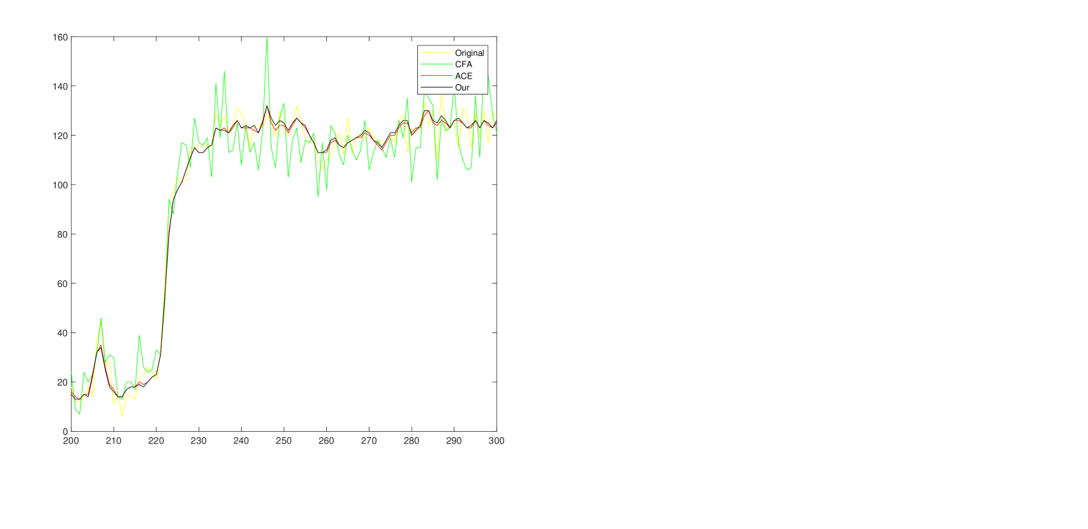
Figure 7: 1D intensity profile passing through the red line in Fig. 6a.

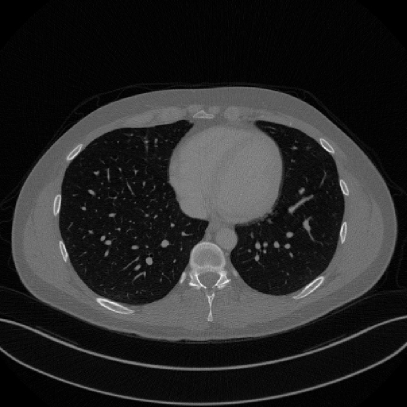
(a) Original

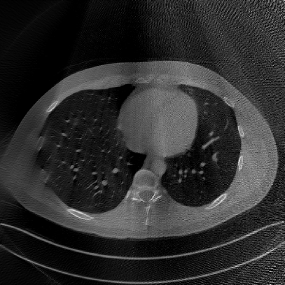
(b) CFA

(c) ACE

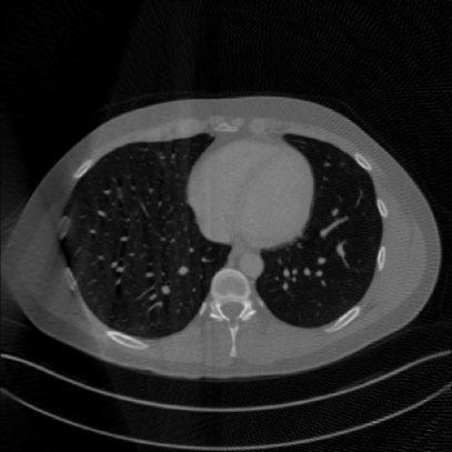
(d) Ours

Figure 8: CT images reconstructed from super-short-scan fan-beam projection data.

III-C Additional discrete schemes

In order to implement our CT reconstruction algorithms, we need to give the discrete definitions of the derivatives $\frac{\partial g_{c}(\lambda,\gamma)}{\partial\lambda}$ and $\frac{\partial g_{c}(\lambda,\gamma)}{\partial\gamma}$ in equation (23), $\frac{\partial g_{l}(\lambda,u)}{\partial\lambda}$ and $\frac{\partial g_{l}(\lambda,u)}{\partial u}$ in equation (26), $\frac{g_{f}(\lambda,u,w)}{\partial\lambda}$, $\frac{g_{f}(\lambda,u,w)}{\partial u}$ and $\frac{g_{f}(\lambda,u,w)}{\partial w}$ in equation (33), and $\frac{g_{c}(\lambda,\alpha,w)}{\partial\lambda}$ and $\frac{g_{c}(\lambda,\alpha,w)}{\partial\alpha}$ in equation (39), the Hilbert filters $h_{H}(u)$ in equations (27) and (34), $h_{H}(\sin(\gamma))$ in equation (24) and $h_{H}(\sin(\alpha))$ in equation (40), and the weighting functions $\varpi_{1}(\underline{x},\lambda)$ in equation (21) and $\varpi_{2}(\underline{x},\lambda)$ in equation (22).

Let

$$\gamma_{i}= i\nabla\gamma,~{}~{}i=-N,-N+1,...,0,...,N-1,N,$$ (43)

$$\alpha_{i}= i\nabla\alpha,~{}~{}i=-N,-N+1,...,0,...,N-1,N,$$

$$u_{j}= j\nabla u,~{}~{}j=-M,-M+1,...,0,...,M-1,M,$$

$$w_{k}= k\nabla w,~{}~{}k=-L,-L+1,...,0,...,L-1,L$$

be the discrete coordinates of the detectors and

$$\lambda_{s}=s\nabla\lambda,~{}~{}s=0,1,...,P$$ (44)

be the discrete sampling angles. To avoid the space shift in the reconstructed images, we use the centered difference schemes to calculate the derivatives:

$$\frac{\partial g_{c}(\lambda_{s},\gamma)}{\partial\lambda}= \frac{g_{c}(\lambda_{s+1},\gamma)-g_{c}(\lambda_{s-1},\gamma)}{2\nabla\lambda},$$ (45)

$$\frac{\partial g_{c}(\lambda,\gamma_{i})}{\partial\gamma}= \frac{g_{c}(\lambda,\gamma_{i+1})-g_{c}(\lambda,\gamma_{i-1})}{2\nabla\gamma},$$

$$\frac{\partial g_{l}(\lambda_{s},u)}{\partial\lambda}= \frac{g_{l}(\lambda_{s+1},u)-g_{l}(\lambda_{s-1},u)}{2\nabla\lambda},$$

$$\frac{\partial g_{l}(\lambda,u_{j})}{\partial\lambda}= \frac{g_{l}(\lambda,u_{j+1})-g_{l}(\lambda,u_{j-1})}{2\nabla u},$$

$$\frac{g_{f}(\lambda_{s},u,w)}{\partial\lambda}= \frac{g_{f}(\lambda_{s+1},u,w)-g_{f}(\lambda_{s-1},u,w)}{2\nabla\lambda},$$

$$\frac{g_{f}(\lambda,u_{j},w)}{\partial u}= \frac{g_{f}(\lambda,u_{j+1},w)-g_{f}(\lambda,u_{j-1},w)}{2\nabla u},$$

$$\frac{g_{f}(\lambda,u,w_{k})}{\partial u}= \frac{g_{f}(\lambda,u,w_{k+1})-g_{f}(\lambda,u,w_{k-1})}{2\nabla w},$$

$$\frac{g_{c}(\lambda_{s},\alpha,w)}{\partial\lambda}= \frac{g_{c}(\lambda_{s+1},\alpha,w)-g_{c}(\lambda_{s-1},\alpha,w)}{2\nabla\lambda},$$

$$\frac{g_{c}(\lambda,\alpha_{i},w)}{\partial\alpha}= \frac{g_{c}(\lambda,\alpha_{i+1},w)-g_{c}(\lambda,\alpha_{i-1},w)}{2\nabla\alpha}.$$

Let $b$ denote a cut-off frequency for the Hilbert filter $h_{H}(u)$. Then, we may write [29]:

$$k_{H}(u) \approx-\int_{-b}^{b}i\operatorname{sgn}(\sigma)e^{i2\pi\sigma u}d\sigma$$ (46)

$$=\int_{-b}^{0}ie^{i2\pi\sigma u}d\sigma-\int_{0}^{b}ie^{i2\pi\sigma u}d\sigma$$

$$=\left[\frac{1}{2\pi u}e^{i2\pi\sigma t}\right]_{\sigma=-b}^{0}-\left[\frac{1}{2\pi u}e^{i2\pi\sigma t}\right]_{\sigma=0}^{b}$$

$$=\frac{1}{2\pi u}(1-e^{-i2\pi bu}-e^{i2\pi bu}+1)$$

$$=\frac{1}{2\pi u}(2-2\cos(2\pi bu))$$

$$=\frac{1}{\pi u}(1-\cos(2\pi bu)).$$

For $h_{H}(\sin(\gamma))$ and $h_{H}(\sin(\gamma))$, we have

$$h_{H}(\sin(\gamma))=\frac{\gamma}{\sin(\gamma)}h_{H}(\gamma)=\frac{1-\cos(2\pi b\gamma)}{\pi\sin(\gamma)}$$ (47)

and so

$$h_{H}(\sin(\alpha))=\frac{1-\cos(2\pi b\alpha)}{\pi\sin(\alpha)}.$$ (48)

In this paper, we set $b=1/(2\nabla u),1/(2\nabla\gamma)$ and $1/(2\nabla\alpha)$ for $h_{H}(u)$, $h_{H}(\sin(\gamma))$ and $h_{H}(\sin(\alpha))$, respectively. Therefore, the discrete definitions of the Hilbert filters are:

$$k_{H}(u_{j})= \frac{1-\cos(\pi u_{j}/\nabla u)}{\pi u_{j}},$$ (49)

$$h_{H}(\sin(\gamma_{i}))= \frac{1-\cos(\pi\gamma_{i}/\nabla\gamma)}{\pi\sin(\gamma_{i})},$$

$$h_{H}(\sin(\alpha_{i}))= \frac{1-\cos(\pi\alpha_{i}/\nabla\alpha)}{\pi\sin(\alpha_{i})}.$$

For the weighting functions $\varpi_{1}(\underline{x},\lambda)$ and $\varpi_{2}(\underline{x},\lambda)$, since the endpoints $\underline{a}(\lambda(\underline{x},\lambda_{0}))$ and $\underline{a}(\lambda(\underline{x},\lambda_{P}))$ may not coincide with the sampling points $a(\lambda_{s})$, we need to interpolate them at the endpoints of the sampling angles $\lambda(\underline{x},\lambda_{0})$ and $\lambda(\underline{x},\lambda_{P})$. Let

$$s(\underline{x},\lambda_{0})= (\lambda(\underline{x},\lambda_{0})-\lambda_{0})/\nabla\lambda,$$ (50)

$$\lfloor s(\underline{x},\lambda_{0})\rfloor= \text{floor}(s(\underline{x},\lambda_{0})),$$

$$\lceil s(\underline{x},\lambda_{0})\rceil= \text{floor}(s(\underline{x},\lambda_{0}))+1,$$

$$s(\underline{x},\lambda_{P})= (\lambda(\underline{x},\lambda_{P})-\lambda_{0})/\nabla\lambda,$$

$$\lfloor s(\underline{x},\lambda_{P})\rfloor= \text{floor}(s(\underline{x},\lambda_{P})),$$

$$\lceil s(\underline{x},\lambda_{P})\rceil= \text{floor}(s(\underline{x},\lambda_{P}))+1.$$

Then, we set

$$\varpi_{1}(\underline{x},\lambda_{s})= \left\{\begin{array}[]{l}1,~{}~{}~{}~{}~{}~{}~{}~{}~{}~{}~{}~{}~{}~{}~{}~{}\text{if}~{}s\in[0,\lfloor s(\underline{x},\lambda_{0})\rfloor],\\ s-\lfloor s(\underline{x},\lambda_{0})\rfloor,~{}\text{if}~{}s\in(\lfloor s(\underline{x},\lambda_{0})\rfloor,\lceil s(\underline{x},\lambda_{0})\rceil),\\ 0,~{}~{}~{}~{}~{}~{}~{}~{}~{}~{}~{}~{}~{}~{}~{}~{}\text{else},\end{array}\right.$$ (51)

$$\varpi_{2}(\underline{x},\lambda_{s})= \left\{\begin{array}[]{l}1,~{}~{}~{}~{}~{}~{}~{}~{}~{}~{}~{}~{}~{}~{}~{}~{}~{}\text{if}~{}s\in[\lceil s(\underline{x},\lambda_{P})\rceil,P],\\ s-\lfloor s(\underline{x},\lambda_{P})\rfloor,~{}\text{if}~{}s\in(\lfloor s(\underline{x},\lambda_{P})\rfloor,\lceil s(\underline{x},\lambda_{P})\rceil),\\ 0,~{}~{}~{}~{}~{}~{}~{}~{}~{}~{}~{}~{}~{}~{}~{}~{}~{}\text{else},\end{array}\right.$$

where $\lambda(\underline{x},\lambda_{0})$ and $\lambda(\underline{x},\lambda_{P})$ can be calculated via Appendix B.

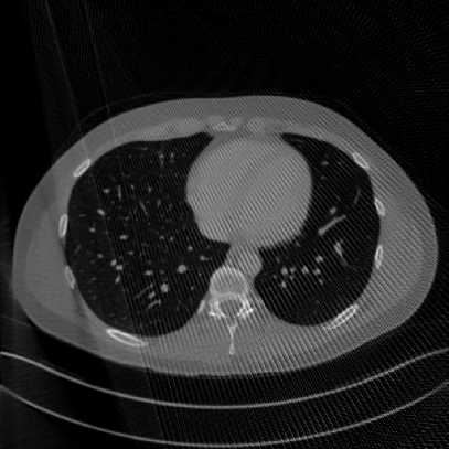
(a)

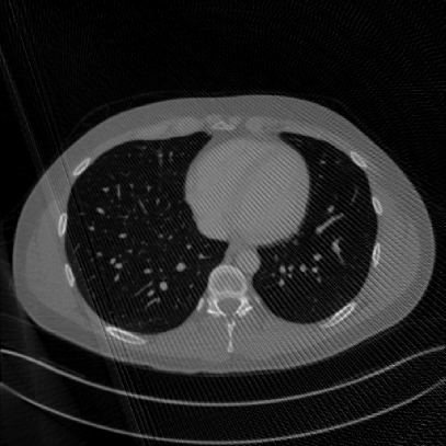
(b)

(c)

(d)

(a) $\beta$=[0:210]

(b) $\beta$=[0:220]

(c) $\beta$=[0:230]

(d) $\beta$=[0:240]

Figure 9: CT images reconstructed from fan-beam projections with different $\beta$. The images in the first row are reconstructed by ACE and in the second row by ours.

(a) var=1

(b) var=10

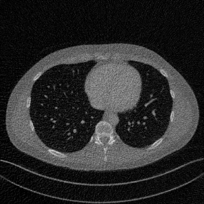
(c) var=100

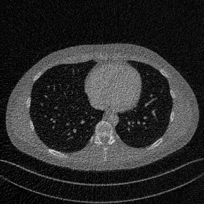
(d) var=200

Figure 10: CT images reconstructed from noisy short-scan fan-beam projection data with different variances.

IV Experimental Results

In this section, we give some simulation results to verify the effectiveness of our algorithms. For 2D fan-beam CT reconstructions, we do the experiments on the simulated projection data measured by equi-angular curved-line detectors while for 3D circle cone-beam, the simualted projection data measured by flat-plane detectors are used to reconstruct CT images. The codes for implementing our methods can be downloaded from https://github.com/wangwei-cmd/arc-based-CT-reconstruction. We also provide the codes that implement the compared methods coded by ourselves in this paper.

IV-A Fan-beam with curved-line detectors

In this subsection, we present some CT images reconstructed from the fan-beam projection data measured by equi-angular curved-line detectors under short-scan and super-short-scan trajectories, and compare the results with those of the conventional fan-beam algorithm with Parker-extended weighting function (CFA) [16] and Noo’s algorithm (ACE) [17].

To test the performances of our method and the compared algorithms, we randomly choose 500 full dose CT images (of size $512\times 512$) from “the 2016 NIH-AAPM-Mayo Clinic Low Dose CT Grand Challenge” [30] as the original images. The parameters for the fan-beam CT with the equi-angular curved-line detector are set as follows: $R_{o}=500$, $R_{m}=\sqrt{2}\times 256$ and so

$$\gamma_{m}=\arctan(R_{m}/R_{o})=35.90^{\circ}.$$

We set $\gamma=[-36:0.1:36]\times\pi/180$ for the sampling positions on the $\gamma$ coordinate. For the sampling positions on the $\lambda$ coordinate, we set

$$\lambda=[0:1:180+2\times 36]\times\pi/180$$

for short-scan and

$$\lambda=[0:1:180]\times\pi/180$$

for super-short scan. The hyper-parameter $d$ in ACE [17] is set as $d=6\times\pi/180$.

In Fig. 6, we show one set of CT images reconstructed by CFA, ACE and ours from the short-scan fan-beam projection data. We can observe that the visual effects of the reconstructed images by ACE and ours are very similar while that by CFA has a lot of artifacts. To objectively estimate the qualities of the reconstructed images by the three methods, the average peak signal to noise ratio (PSNR) and structural similarity (SSIM) of the 500 reconstructed CT images are listed in Table I. We can see that our method has a slightly higher average PSNR and SSIM than those of ACE. The average PSNR and SSIM of CFA are far lower than those of ACE and ours. It’s because that the CFA algorithm needs higher sampling rate on the $\lambda$ coordinate. By experiments, we find that when setting $\lambda=[0:0.25:180+2\times 36]\times\pi/180$, the PSNR and SSIM of CFA can be raised to the same level of ACE and ours.

In Fig. 7, we plot the 1D line intensity profile passing through the red line in Fig. 6a. We can observe that the intensity lines of ACE and ours are almost coincident and resemble more closely to the one of the original compared to that of CFA.

In Fig. 8, a set of CT images reconstructed by CFA, ACE and ours from the super-short-scan fan-beam projections are presented. We can observe that all the three images reconstructed by CFA, ACE and ours suffer from intensity inhomogeneity on the left part of the reconstructed images due to the data incompleteness. Moreover, the stripe visual effect can be easily observed in Fig. 8b. In Fig. 8c, a vertical line can be observed. This may be caused by data missing at the endpoints of the scanning arcs. Compared to CFA and ACE, our method has the best visual effect as can be seen from Fig. 8d. In Table II, the average PSNR and SSIM of the CT images reconstructed by CFA, ACE and ours are, respectively, listed, from which we can see that our method has the highest average PSNR and SSIM.

To better demonstrate the artifacts of ACE caused by data incompleteness, the CT images corresponding to $\lambda=[0:1:210]\times\pi/180$, $\lambda=[0:1:220]\times\pi/180$, $\lambda=[0:1:230]\times\pi/180$ and $\lambda=[0:1:240]\times\pi/180$ reconstructed by ACE and ours are shown in Fig. 9. We can observe that when the range of $\lambda$ is lower than $240^{\circ}$, some stripe visual effects can be observed in the CT images reconstructed by ACE. As the range of $\lambda$ exceeds $240^{\circ}$, the artifacts of ACE caused by the data missing almost disappear. For our method, even $\lambda=[0:1:210]\times\pi/180$, there exists no stripe artifact in the reconstructed CT images.

(a)

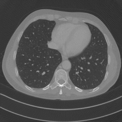
(b)

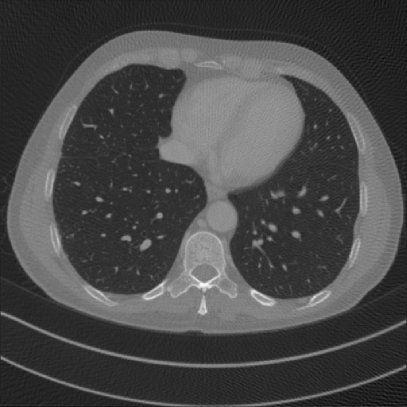
(c)

(d)

(e)

(f)

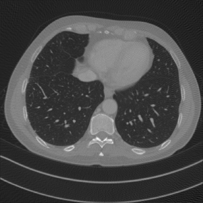
(g)

(h)

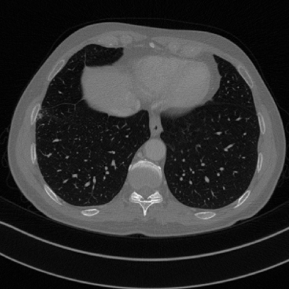
(i)

(j)

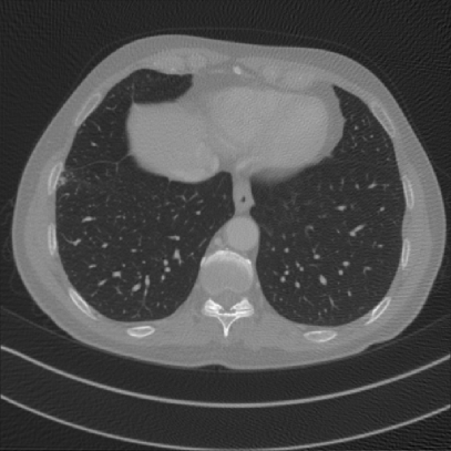
(k)

(l)

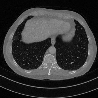
(a) Original

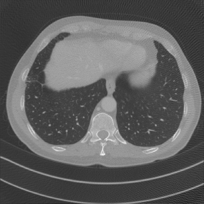
(b) FDK

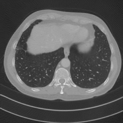
(c) ACE

(d) Ours

Figure 11: Sliced CT images reconstructed from short-scan circle cone-beam projection data.

To test the performances of our method when the projection data is corrupted by noise, we add Poisson and Gaussian noise to the short-scan projections via the following formulas [31]:

$$g =\exp(-g/M),$$ (52)

$$g =g+I_{0}*poission(g)+I_{0}*Gaussin(m,var/I_{0}),$$

$$g =\log(I_{0}/g)*M,$$

where $M$ is the maximal value of the projection data $g$, $m$ and $var$ are the mean and variance of the Gaussian noise, respectively, $I_{0}$ is the average photon count for the Poisson noise. In this experiment, we set $I_{0}=10^{6}$, $m=0$, and $var=1,10,100,200$, respectively. The reconstructed images from the noisy projection data are shown in Fig. 10. We can observe that as the variance $var$ increases, the reconstructed CT image has more noise.

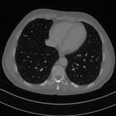
(a)

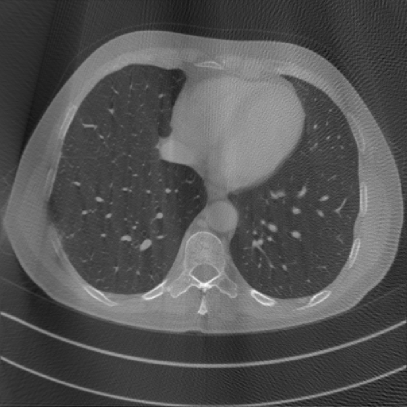
(b)

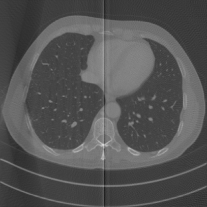
(c)

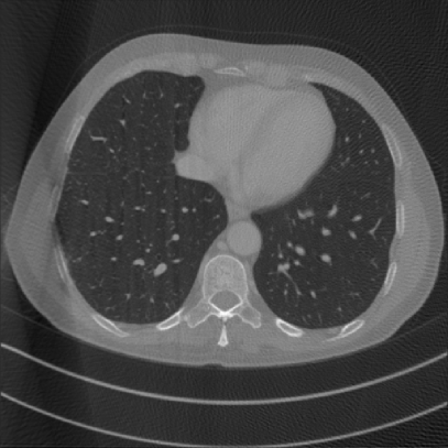
(d)

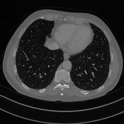
(e)

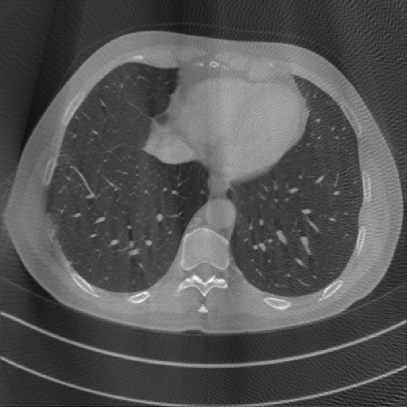
(f)

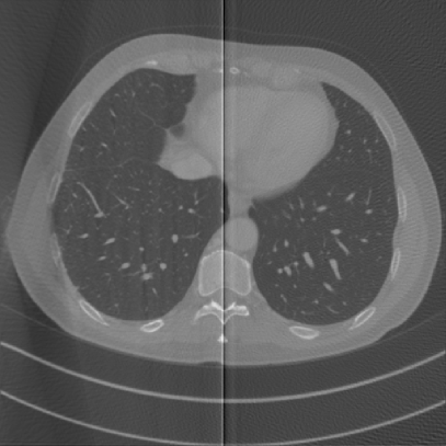
(g)

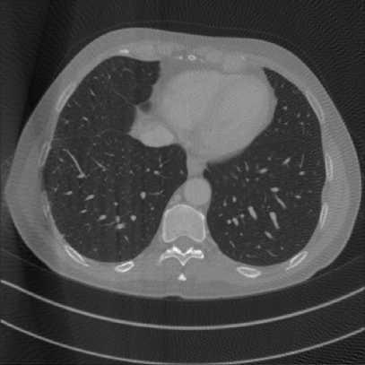
(h)

(i)

(j)

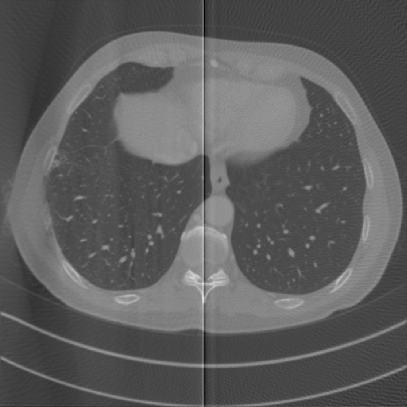
(k)

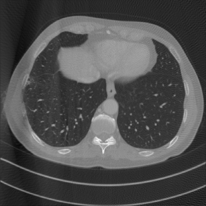
(l)

(a) Original

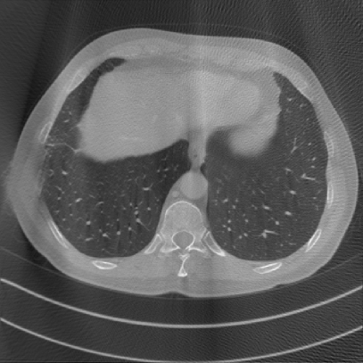
(b) FDK

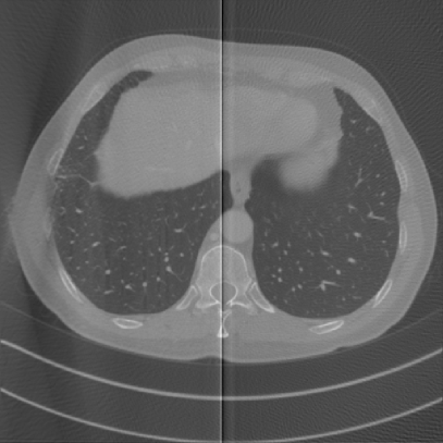
(c) ACE

(d) Ours

Figure 12: Sliced CT images reconstructed from super-short-scan circle cone-beam projection data.

TABLE I: The Averaged PSNR and SSIM of CT Images Reconstructed by CFA, ACE and Ours from Fan-Beam Short-Scan Projection Data.

	PSNR	SSIM
CFA	18.74 $\pm$0.52	0.47$\pm$0.01
ACE	34.66$\pm$0.60	0.83$\pm$0.01
ours	34.78 $\pm$0.62	0.84$\pm$0.01

TABLE II: The Averaged PSNR and SSIM of CT Images Reconstructed by CFA, ACE and Ours from Fan Beam Super-Short-Scan Projection Data.

	PSNR	SSIM
CFA	18.51 $\pm$0.45	0.43$\pm$0.01
ACE	25.53$\pm$0.70	0.45$\pm$0.03
ours	27.64 $\pm$0.94	0.66$\pm$0.02

IV-B Circle cone-beam with flat-plane detectors

In this subsection, we give some CT images reconstructed from the circle cone-beam projection data measured by flat-plane detectors to very the effectiveness of our method, and compare the results with those of the Feldkamp-Davis-Kress (FDK) algorithm [7] and Noo’s algorithm (ACE) [17], where we extend the weighting function of ACE such that it can be used to reconstruct circle cone-beam CT images.

To test the performances of our method and the compared algorithms, we randomly choose 2500 full dose CT images (of size $512\times 512$) from “the 2016 NIH-AAPM-Mayo Clinic Low Dose CT Grand Challenge” [30] and use them to assemble 50 objects of size $512\times 512\times 50$ as the original images.

The parameters for the circle cone-beam CT with the flat-plane detector are set as follows: $u=[-494:1:494]$, $v=[-54:1:54]$, $R_{o}=1000$, and

$$D=\text{ceil}(R_{o}+\sqrt{2}\times 256)=1363.$$

For the sampling positions on the $\lambda$ coordinate, we set

$$\lambda=[0:1:180+2\times 20]\times\pi/180$$

for short-scan and

$$\lambda=[0:1:180]\times\pi/180$$

for super-short-scan. The $26$th slice of the images of the object is assumed to lie in the plane $z=0$ (i.e. the plane formed by the trajectory of the X-ray source). The hyper-parameter $d$ in ACE [17] is set as $d=10\times\pi/180$.

In Fig. 11, we present some sliced CT images of one object reconstructed by FDK, ACE and ours from the short-scan circle cone-beam projection data. We can observe that there exist some stripe artifacts in the CT images reconstructed by FDK. The visual effects of the CT images reconstructed by ACE and ours are very similar. We also use the PSNR and SSIM to measure the similarities of the reconstructed CT images and the original. From Table III, we can observe that the average PSNR and SSIM of our method are slightly higher than that of ACE and are higher than that of CFA, which coincides with our observations.

In Fig. 12, some sliced CT images of one object reconstructed by FDK, ACE and ours from the super-short-scan circle cone-beam projection data are shown. From Fig. 12b, we can see that some stripe visual artifacts exit in the CT images reconstructed by FDK. Moreover, the left hand side parts of the CT images reconstructed by FDK suffer from severe intensity inhomogeneity. From Fig. 12b, we can observe that there also exit some undesirable vertical lines in the CT images reconstructed by ACE, which may be caused by the data incompleteness. Compared to Fig. 12b and Fig. 12c, the CT images reconstructed by our method suffer from less intensity inhomogeneity and their visual effects are the best as shown in Fig. 12d. The PSNR and SSIM are used to evaluate the qualities of the reconstructed images and listed in Table IV. We can see that our method has the highest PSNR and SSIM compared to CFA and ACE.

TABLE III: The Averaged PSNR and SSIM of CT Images Reconstructed by FDK, ACE and Ours from Circle Cone-Beam Short-Scan Projection Data.

	PSNR	SSIM
CFA	29.90 $\pm$1.17	0.66$\pm$0.03
ACE	31.10$\pm$1.79	0.67$\pm$0.04
ours	31.16 $\pm$1.79	0.68$\pm$0.04

TABLE IV: The Averaged PSNR and SSIM of CT Images Reconstructed by FDK, ACE and Ours from Circle Cone-Beam Super-Short-Scan Projection Data.

	PSNR	SSIM
CFA	24.69 $\pm$1.83	0.49$\pm$0.04
ACE	26.11$\pm$1.87	0.52$\pm$0.05
ours	27.99 $\pm$1.84	0.59$\pm$0.04

V Conclusion

In this paper, we proposed a new weighting function to deal with the redundant projection data for the arc based fan-beam CT algorithm, which was obtained via applying Katsevich’s helical CT formula [21] to 2D fan-beam CT reconstruction. By extending the arc based algorithm to circle cone-beam geometry with the proposed weighting function, we also obtained a new FDK-similar algorithm for circle cone-beam CT reconstruction. Experiments showed that our methods can obtained higher PSNR and SSIM compared to the related algorithms when the scanning trajectories are super-short-scan.

Appendix A Algorithm for circle cone-beam CT with flat-plane detector

Figure 13: Relation between $\gamma$ and the flat-plane detector coordinates.

As can be observed from Fig. 13, we have

$$\underline{e}_{u}(\lambda)=\frac{\overrightarrow{A_{4}A_{3}}}{||\overrightarrow{A_{4}A_{3}}||},~{}\underline{e}_{v}(\lambda) =\frac{\overrightarrow{A_{1}A_{2}}}{\overrightarrow{A_{1}A_{2}}},~{}\underline{e}_{w}(\lambda)=\frac{\overrightarrow{A_{2}A_{3}}}{\overrightarrow{A_{2}A_{3}}},$$ (53)

$$||\overrightarrow{A_{4}A_{3}}||=u,~{}||\overrightarrow{A_{5}A_{3}}||=\bar{u}, ~{}||\overrightarrow{A_{2}A_{3}}||=w,~{}||\overrightarrow{A_{2}A_{3}}||=D,$$

$$\angle A_{4}A_{1}A_{3}=\alpha, ~{}~{}~{}~{}~{}~{}~{}~{}~{}~{}\angle A_{5}A_{1}A_{4}=\bar{\gamma}.$$

We also have $\tan(\alpha+\bar{\gamma})=\frac{||\overrightarrow{A_{5}A_{3}}||}{||\overrightarrow{A_{1}A_{3}}||}=\frac{\bar{u}}{\sqrt{D^{2}+w^{2}}}$ and so

$$\mathrm{d}\bar{\gamma}=\frac{\cos^{2}(\alpha+\bar{\gamma})}{\sqrt{D^{2}+w^{2}}}\mathrm{d}\bar{u}=\frac{\sqrt{D^{2}+w^{2}}}{D^{2}+w^{2}+\bar{u}^{2}}\mathrm{d}\bar{u}.$$ (54)

By the Law of Sines, we have

$$\sin\bar{\gamma}= ||\overrightarrow{A_{5}A_{4}}||\frac{\sin(\angle A_{1}A_{5}A_{3})}{||\overrightarrow{A_{1}A_{4}}||}$$ (55)

$$= \frac{\sqrt{D^{2}+w^{2}}(\bar{u}-u)}{\sqrt{D^{2}+w^{2}+\bar{u}^{2}}\sqrt{D^{2}+w^{2}+u^{2}}}.$$

Therefore,

$$h_{H}(\sin\bar{\gamma})=\frac{\sqrt{D^{2}+w^{2}+\bar{u}^{2}}\sqrt{D^{2}+w^{2}+u^{2}}}{\sqrt{D^{2}+w^{2}}}h_{H}(\bar{u}-u).$$ (56)

Note that $\underline{\theta}(\lambda,u,w)=\frac{\overrightarrow{A_{1}A_{4}}}{||\overrightarrow{A_{1}A_{4}}||}$ and so $\cos\bar{\gamma}\underline{\theta}+\sin\bar{\gamma}\underline{\theta}^{\bot}=\frac{\overrightarrow{A_{1}A_{5}}}{||\overrightarrow{A_{1}A_{5}}||}$. Substituting equations (54) and (56) into equation (18), we can obtain

$$g^{F}(\lambda, \underline{\theta}(\lambda,u,w))=-\frac{\sqrt{u^{2}+D^{2}+w^{2}}}{D}\times$$ (57)

$$\int_{-u_{m}}^{u_{m}}\mathrm{d}\bar{u}\frac{D}{\sqrt{\bar{u}^{2}+D^{2}+w^{2}}}h_{H}(u-\bar{u})g_{1}(\lambda,\bar{u},w),$$

From Fig. 4, we can observe that

$$\|\underline{x}-\underline{a}(\lambda)\|= \sqrt{(u^{*})^{2}+(w^{*})^{2}+D^{2}}\frac{(\underline{x}-\underline{a}(\lambda))\cdot\underline{e}_{v}(\lambda)}{D}$$ (58)

$$= \frac{\sqrt{(u^{*})^{2}+(w^{*})^{2}+D^{2}}}{D}(R_{o}+\underline{x}\cdot\underline{e}_{v}(\lambda)).$$

Substituting equation (58) into equation (17), we can get

$$f(\underline{x})= -\frac{D}{\sqrt{D^{2}+(w^{*})^{2}+(u^{*})^{2}}}\times$$ (59)

$$\frac{1}{2\pi}\int_{\lambda_{0}}^{\lambda_{P}}\mathrm{d}\lambda\frac{\varpi_{3d}(\underline{x},\lambda)}{v^{*}(\underline{x},\lambda)}g_{2}\left(\lambda,u^{*},w^{*}\right).$$

Canceling the factors $-\frac{\sqrt{u^{2}+D^{2}+w^{2}}}{D}$ and $-\frac{D}{\sqrt{D^{2}+(w^{*})^{2}+(u^{*})^{2}}}$ in equations (57) and (59), we obtain the algorithm for circle cone-beam CT with the flat-plane detector.

Appendix B Algorithm for calculating one endpoint of a chord

Let $(R_{o}\cos\lambda_{0},R_{o}\sin\lambda_{0})$ and $(R_{o}\cos\lambda_{1},R_{o}\sin\lambda_{1})$ be the two end-points of a chord on a circle with radius $r=R_{o}$ and $(x_{1},x_{2})$ be a point on the chord. Then, we have

$$R_{o}(\cos\lambda_{1}-\cos\lambda_{0}) =t*(x_{1}-R_{o}\cos\lambda_{0}),$$ (60)

$$R_{o}(\sin\lambda_{1}-\sin\lambda_{0}) =t*(x_{2}-R_{o}\sin\lambda_{0}),$$

where $t\in[0,1]$. Solving equation set (60), we have

$$\cos\lambda_{1}=\{R_{o}(-R_{o}^{2}+x_{1}^{2}+x_{2}^{2})\cos\lambda_{0}-$$ (61)

$$~{}~{}~{}~{}~{}~{}~{}~{}2x_{1}(-R_{o}^{2}+x_{1}R_{o}\cos\lambda_{0}+x_{2}R_{o}\sin\lambda_{0})\}/$$

$$\{R_{o}(R_{o}^{2}+x_{1}^{2}+x_{2}^{2}-2x_{1}R_{o}\cos\lambda_{0}-2x_{2}R_{o}\sin\lambda_{0})\},$$

$$\sin\lambda_{1}=\{R_{o}(-R_{o}^{2}+x_{1}^{2}+x_{2}^{2})\sin\lambda_{0}-$$

$$~{}~{}~{}~{}~{}~{}~{}~{}2x_{2}(-R_{o}^{2}+x_{1}R_{o}\cos\lambda_{0}+x_{2}R_{o}\sin\lambda_{0})\}/$$

$$\{R_{o}(R_{o}^{2}+x_{1}^{2}+x_{2}^{2}-2x_{1}R_{o}\cos\lambda_{0}-2x_{2}R_{o}\sin\lambda_{0})\}.$$

Thus, we can get $\lambda_{1}$ by $\lambda_{1}=\arccos(\cos\lambda_{1})$, where $\lambda_{1}$ needs to be changed by $\lambda_{1}=2\pi-\lambda_{1}$ when $\sin\lambda_{1}<0$.

References

- [1] G. Wang, T. H. Lin, P. C. Cheng, and D. M. Shinozaki, “A General Cone-Beam Reconstruction Algorithm,” IEEE Transactions on Medical Imaging, vol. 12, no. 3, pp. 486–496, 1993.
- [2] K. Stierstorfer, A. Rauscher, J. Boese, H. Bruder, S. Schaller, and T. Flohr, “Weighted FBP - a Simple Approximate 3D FBP Algorithm for Multislice Spiral CT With Good Dose Usage for Arbitrary Pitch,” Physics in Medicine and Biology, vol. 49, no. 11, pp. 2209–2218, JUN 7 2004.
- [3] F. Noo, S. Hoppe, F. Dennerlein, G. Lauritsch, and J. Hornegger, “A New Scheme for View-Dependent Data Differentiation in Fan-Beam and Cone-Beam Computed Tomography,” Physics in Medicine and Biology, vol. 52, no. 17, pp. 5393–5414, 2007.
- [4] A. A. Zamyatin, K. Taguchi, and M. D. Silver, “Practical Hybrid Convolution Algorithm for Helical CT Reconstruction,” IEEE Transactions on Nuclear Science, vol. 53, no. 1, pp. 167–174, 2006.
- [5] H. Kudo, T. Rodet, F. Noo, and M. Defrise, “Exact and Approximate Algorithms for Helical Cone-Beam CT,” Physics in Medicine and Biology, vol. 49, no. 13, pp. 2913–2931, 2004.
- [6] X. Y. Tang, J. Hsieh, R. A. Nilsen, S. Dutta, D. Samsonov, and A. Hagiwara, “A Three-Dimensional-Weighted Cone Beam Filtered Backprojection (CB-FBP) Algorithm for Image Reconstruction in Volumetric CT - Helical Scanning,” Physics in Medicine and Biology, vol. 51, no. 4, pp. 855–874, 2006.
- [7] L. FELDKAMP, L. DAVIS, and J. KRESS, “Practical Cone-Beam Algorithm,” Journal of the Optical Society of America a-Optics Image Science and Vision , vol. 1, no. 6, pp. 612–619, 1984.
- [8] L. F. Yu, X. C. Pan, and C. A. Pelizzari, “Image Reconstruction With a Shift-Variant Filtration in Circular Cone-Beam CT,” International Journal of Imaging Systems and Technology, vol. 14, no. 5, pp. 213–221, 2004.
- [9] H. Kudo, F. Noo, M. Defrise, and R. Clackdoyle, “New Super-Short-Scan Algorithms for Fan-Beam and Cone-Beam Reconstruction,” in IEEE Nuclear Science Symposium and Medical Imaging Conference, 2003, pp. 902–906.
- [10] S. Tang and X. Tang, “Axial Cone-Beam Reconstruction by Weighted BPF/DBPF and Orthogonal Butterfly Filtering,” IEEE Transactions on Biomedical Engineering, vol. 63, no. 9, pp. 1895–1903, 2016.
- [11] S. Tang, K. Huang, Y. Cheng, T. Niu, and X. Tang, “Three-Dimensional Weighting in Cone Beam FBP Reconstruction and Its Transformation Over Geometries,” IEEE Transactions on Biomedical Engineering, vol. 65, no. 6, pp. 1235–1244, JUN 2018.
- [12] X. Y. Tang, J. Hsieh, A. Hagiwara, R. A. Nilsen, J. B. Thibault, and E. Drapkin, “A Three-Dimensional Weighted Cone Beam Filtered Backprojection (CB-FBP) Algorithm for Image Reconstruction in Volumetric CT Under a Circular Source Trajectory,” Physics in Medicine and Biology, vol. 50, no. 16, pp. 3889–3905, 2005.
- [13] B. K. P. Horn, “Fan-Beam Reconstruction Methods,” Proceedings of the IEEE, vol. 67, no. 12, pp. 1616–1623, 1979.
- [14] G. T. Herman and A. Naparstek, “Fast Image-Reconstruction Based on a Radon Inversion Formula Appropriate for Rapidly Collected Data,” SIAM Journal on Applied Mathematics, vol. 33, no. 3, pp. 511–533, 1977.
- [15] D. PARKER, “Optimal Short Scan Convolution Reconstruction for Fanbeam CT,” Medical Physics, vol. 9, no. 2, pp. 254–257, 1982.
- [16] M. D. Silver, “A Method for Including Redundant Data in Computed Tomography,” Medical Physics, vol. 27, no. 4, pp. 773–774, 2000.
- [17] F. Noo, M. Defrise, R. Clackdoyle, and H. Kudo, “Image Reconstruction From Fan-Beam Projections on Less Than a Short Scan,” Physics in Medicine and Biology, vol. 47, no. 14, pp. 2525–2546, JUL 21 2002.
- [18] G. H. Chen, “A New Framework of Image Reconstruction From Fan Beam Projections,” Medical Physics, vol. 30, no. 6, pp. 1151–1161, 2003.
- [19] F. Noo, R. Clackdoyle, and J. Pack, “A Two-Step Hilbert Transform Method for 2D Image Reconstruction,” Physics in Medicine and Biology, vol. 49, no. 17, pp. 3903–3923, SEP 7 2004.
- [20] Y. Zou and X. Pan, “Exact Image Reconstruction on PI-Lines From Minimum Data in Helical Cone-Beam CT,” Physics in Medicine and Biology, vol. 49, no. 6, pp. 941–959, MAR 21 2004.
- [21] A. Katsevich, “An Improved Exact Filtered Backprojection Algorithm for Spiral Computed Tomography,” Advances in Applied Mathematics, vol. 32, no. 4, pp. 681–697, MAY 2004.
- [22] J. You and G. L. Zeng, “Hilbert Transform Based FBP Algorithm for Fan-Beam CT Full and Partial Scans,” IEEE Transactions on Medical Imaging, vol. 26, no. 2, pp. 190–199, 2007.
- [23] A. Katsevich, “A Note on Computing the Derivative at a Constant Direction,” Physics in Medicine and Biology, vol. 56, no. 4, pp. N53–N61, 2011.
- [24] K. Taguchi, B. S. S. Chiang, and M. D. Silver, “A New Weighting Scheme for Cone-Beam Helical CT to Reduce the Image Noise,” Physics in Medicine and Biology, vol. 49, no. 11, pp. 2351–2364, 2004.
- [25] A. Katsevich, “Theoretically Exact Filtered Backprojection-Type Inversion Algorithm For Spiral CT,” SIAM Journal on Applied Mathematics, vol. 62, no. 6, pp. 2012–2026, AUG 2 2002.
- [26] L. Yu, D. Xia, Y. Zou, E. Y. Sidky, J. Bian, and X. Pan, “A Rebinned Backprojection-Filtration Algorithm for Image Reconstruction in Helical Cone-Beam CT,” Physics in Medicine and Biology, vol. 52, no. 18, pp. 5497–5508, 2007.
- [27] H. Schoendube, K. Stierstorfer, and F. Noo, “Accurate Helical Cone-Beam CT Reconstruction With Redundant Data,” Physics in Medicine and Biology, vol. 54, no. 15, pp. 4625–4644, 2009.
- [28] F. Noo, J. Pack, and D. Heuscher, “Exact Helical Reconstruction Using Native Cone-Beam Geometries,” Physics in Medicine and Biology, vol. 48, no. 23, pp. 3787–3818, 2003.
- [29] A. J. Wunderlich, “The Katsevich Inversion Formula for Cone-Beam Computed Tomography,” Ph.D. dissertation, Oregon State University, 2006.
- [30] C. McCollough, “TU-FG-207A-04: Overview of the Low Dose CT Grand Challenge,” Medical Physics, vol. 43, no. 3759-3760, pp. 3759–3760, 2016.
- [31] Y. Liu, J. Ma, Y. Fan, and Z. Liang, “Adaptive-Weighted Total Variation Minimization for Sparse Data Toward Low-Dose X-Ray Computed Tomography Image Reconstruction,” Physics in Medicine and Biology, vol. 57, no. 23, pp. 7923–7956, 2012.