Kolmogorov-Hinze scales in turbulent superfluids
Abstract
When a two-component mixture of immiscible fluids is stirred, the fluids are split into smaller domains with more vigorous stirring. We numerically investigate the sizes of such domains in a fully-developed turbulent state of a two-component superfluid stirred with energy input rate . For the strongly immiscible condition, the typical domain size is shown to be proportional to , as predicted by the Kolmogorov-Hinze theory in classical fluids. For the weakly immiscible condition, quantum effects become pronounced and the power changes from to .
When oil is poured into water and these fluids are stirred, the oil becomes split into droplets in the water. The droplet sizes become smaller with more vigorous stirring. Such disintegration phenomena in multicomponent fluids are ubiquitous in nature, and are important in engineering and industry.
Kolmogorov [1] and Hinze [2] considered the disintegration process of droplets, and estimated the size of droplets in turbulent fluids. In fully-developed turbulence, the energy is input into the system as large-scale eddies, which cascades toward a smaller scale, resulting in the Kolmogorov power law of the energy spectrum [3]. In such turbulent fluids, large-size droplets are unstable because they are susceptible to deformation and disintegration due to the fluctuating pressure of the surrounding fluid. Small droplets are thus produced by the breakup of large droplets, and this breakup process continues to a scale where the turbulent energy to break up the droplets becomes balanced with the droplet energy that sustains their shape. Droplets smaller than this scale coalesce into large droplets. Therefore, there exists a characteristic size for droplets in turbulent fluids, which is referred to as the Kolmogorov-Hinze (KH) scale, given by [2]
| (1) |
where is the interface tension coefficient, is the density of the surrounding fluid, and is the energy input rate to maintain the turbulence. The KH scale has been experimentally verified in various systems [4, 5, 6, 7, 8]. Furthermore, direct numerical simulations have been performed over the last decade [9, 10, 11, 12, 13, 14].
In this Letter, we extend the study of KH scales to a quantum mechanical system: the superfluid turbulence of a two-component Bose-Einstein condensate (BEC). We will show that the KH scale also appears in this superfluid system and is modified by quantum effects. Turbulent behavior in superfluids has been widely studied. For single-component superfluids, a steady or decaying turbulent state exhibits the Kolmogorov power law [15, 16, 17, 18, 19, 20, 21, 22, 23, 24, 25, 26, 27, 28, 29, 30]. The turbulent behavior of gaseous BECs has also been experimentally studied [31, 32, 33], and a power law behavior has been observed recently [34, 35, 36, 37, 38, 39]. A wide variety of systems have been studied theoretically, such as two-dimensional systems [40, 41, 42, 43, 44, 45], dipolar superfluids [46], and boundary layers [47]. Here, we focus on the turbulence in a two-component BEC. Turbulence in multicomponent BECs has been investigated by many researchers [48, 49, 50, 51, 52, 53, 54, 55, 56, 57, 58, 59, 60, 61]. In the context of domain-size scaling in multicomponent BECs, coarsening dynamics following domain formation have been studied extensively [62, 63, 64, 65, 66, 67, 68, 69, 70, 71, 72, 73, 74, 75, 76]. However, the KH scale, i.e., domain-size scaling in conjunction with Kolmogorov turbulence, has not yet been investigated.
The KH scale in Eq. (1) is derived as follows. In a turbulent fluid, a domain undergoes fluctuating pressures that vary over its size , which causes deformation and disintegration of the domain. This pressure difference can be expressed as , where is the velocity difference of the surrounding fluid over a size . Within the inertial range of an isotropic homogeneous turbulence, the statistical average of obeys the Kolmogorov two-thirds law [3], , and hence . On the other hand, a domain tends to sustain its shape and resist disintegration. This sustaining force arises from the interface tension, and the pressure required to deform the domain is estimated to be [77]. Breakup of domains to smaller sizes stops at the scale that satisfies
| (2) |
which gives the KH scale in Eq. (1).
For an immiscible two-component BEC, the interface tension, which arises from the interatomic interaction and quantum pressure, is well-defined, as in classical fluids [78, 79, 80]. Therefore, we expect that the KH scale in Eq. (1) also emerges in two-component BECs, when the thickness of the interface is much smaller than the domain size . However, when is comparable to or larger than , the picture of the interface tension breaks down in the derivation of Eq. (1). The interface thickness is determined by the competition between the quantum pressure and the intercomponent repulsion, and becomes large when the former dominates the latter. Thus, in the limit of large , the mechanism to sustain domains against disintegration originates mainly from the quantum pressure instead of , where and are the atomic number density and mass, respectively. In this case, Eq. (2) gives the characteristic size as
| (3) |
Therefore, in the limit of weak segregation with large , the quantum mechanical effect becomes pronounced and the KH scale is expected to change from the to power law with respect to . In the remainder of this Letter, we will corroborate this prediction using numerical simulations of the coupled Gross-Pitaevskii (GP) equations.
In the mean-field approximation, a two-component BEC at zero temperature is described by the coupled GP equations,
where is the macroscopic wave function for the th component, is the external stirring potential, and with being the -wave scattering length between the th and th components.
The miscibility between the two components is determined by the coupling coefficients . The two superfluids are immiscible and phase separation occurs when is satisfied [81]. In the following, for simplicity, we assume and ; therefore, the immiscible condition reduces to . The phase separation of immiscible components produces an interface, at which excess energy arises, resulting in interface tension. For , the interface tension coefficient is given by [78, 79, 80]
| (5) |
The interface thickness between two components, over which the density of each component changes from 0 to (or to 0), has the form
| (6) |
where is the healing length.
In the following, the length, time, and wave functions are normalized by , , and , respectively, where is the interface thickness defined in Eq. (6) and is the average density of each component. In this unit, the normalized interaction coefficients, and , in the GP equation become [82]
| (7) |
and ; therefore, the interaction coefficients are reduced to the single parameter . The GP equation is numerically solved using the split-step Fourier method [83]. We consider a box of size with a periodic boundary condition, where the nondimensional healing length is . The box is discretized into a mesh, and the spatial resolution is 0.5 . The two components are equally populated, , and the initial state has a uniform density with random phases on each mesh.
To input the large-scale turbulent energy, the system is stirred using plate-shaped potentials given by
| (8) |
where the potential height is taken to be , is the Heaviside step function, and the summation is taken over , , and with , , and , respectively. The three plate-shaped potentials oscillating in the , , and directions produce isotropic turbulence. The maximum Mach number of the plate-shaped potentials is defined as
| (9) |
where is the sound velocity.
To realize a steady turbulent state, the energy must be dissipated on a small length scale. For this purpose, the term is added to the right-hand sides of Eq. (4), where is a positive constant and
| (10) |
This phenomenological dissipation term mimics the viscous term in the Navier-Stokes equation and reduces the energy of the system while maintaining the unitarity [82]. The value of is selected in such a way that energy dissipation occurs predominantly on a scale below those for the inertial range and the domain size. The larger-scale dynamics are not affected by the details of the dissipation, as long as it occurs on a sufficiently small scale [82].
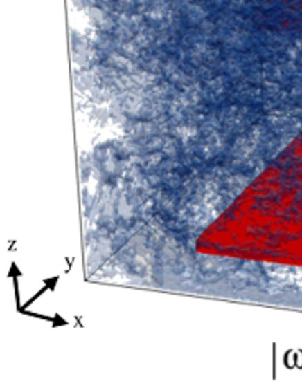
Figure 1(a) shows isodensity surfaces of and after the fully-developed turbulent state is achieved. The two components are separated and domains are formed in each component because of the immiscible condition . The domain sizes in Fig. 1(a) are typically (note that the interface thickness is unity in the present unit), and thus the KH scale is expected to be in the region of Eq. (1) (rather than Eq. (3)), which will be investigated later.
Figures 1(c) and 1(d) show cross-sectional views of the densities and , respectively. Although (or ) largely varies in space due to the phase separation (Fig. 1(c)), the total density far from the stirring potentials is almost uniform (Fig. 1(d)) and density holes arising from quantized vortices are rarely observed, since the velocity of the stirring potential is much lower than the sound velocity of the density waves. This situation is different from the quantum turbulence in a single-component system, in which quantized vortices play a central role in the energy cascade. This difference arises because the vorticity of the mass current is not quantized in the two-component system. To observe this, we define the vorticity of the mass-current velocity as . Figures 1(b) and 1(e) show the distribution of . It is evident from Figs. 1(c) and 1(e) that the vorticity is localized around the interfaces of the domains.
The typical size of the domains can be evaluated from the density correlation function,
| (11) |
where is the density-imbalance distribution and represents the average over the position and the direction of . Figure 2(a) shows the time evolution of . Since the initial wave function has a random distribution, is initially narrow, which then becomes broader and reaches a steady shape for . We have confirmed that the steady shape of is not dependent on the initial state. We define the typical domain size as the full width at half maximum of the correlation function . Figure 2(b) shows the time development of for different values of and . The size decreases with increasing and .
The energy input rate per atom is obtained by
| (12) |
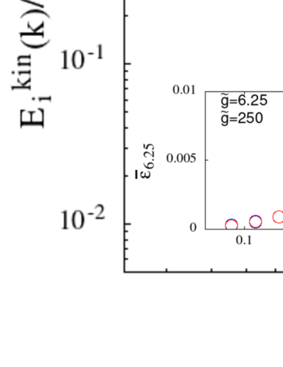
where the time dependence of the potential is given in Eq. (8). The value of (and also ) fluctuates over time due to the random nature of the turbulence. The sinusoidal motion of the plate-shaped potentials also causes periodic fluctuation. Therefore, we take the temporal average of these quantities, and , over a sufficiently long time after the steady turbulent state is achieved. The inset in Fig. 2(c) shows as a function of .
To confirm that the system has reached the Kolmogorov turbulence state, we calculate the kinetic energy spectrum of the incompressible velocity field of the mass current [82], which is shown in Fig. 1(c). Since the Kolmogorov theory predicts , the plots in Fig. 2(c) are compensated by . The length is also rescaled by the domain size to observe the effect of the domains on the energy spectrum. Figure 2(c) shows that the lines of the energy spectra with different and collapse into a single universal line with a slope of on a scale larger than the domain size (), which implies that the Kolmogorov energy cascade occurs on this scale. At the scale of , the energy cascade is arrested by the domains [11], which results in a “bump” in the energy spectrum, as shown in Fig. 2(c). This situation is similar to the case of a single-component system, in which the inertial range is terminated at the scale of the mean distance between quantized vortices [15, 84].
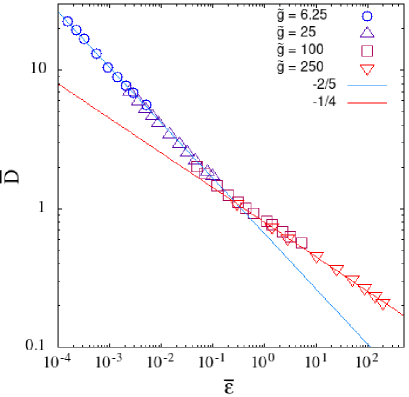
Now we are ready to investigate the KH scales in a turbulent superfluid in the classical and quantum regimes, as given in Eqs. (1) and (3), respectively. The results are shown in Fig. 3, which are the main results obtained in this study. Figure 3 plots the typical domain size versus the energy input rate for various values of the Mach number of the stirring potential and the normalized interaction coefficient . For (note that is normalized by the interface width ), the plots obey the power law , which agrees with the classical KH scale in Eq. (1). This implies that the two components are well separated and the mechanism that sustains the domains against disintegration can be described by the interface tension in this region. For , on the other hand, the plots in Fig. 3 follow the power law , which agrees with the KH scale in the quantum region in Eq. (3) and implies that the mechanism that sustains domains is mainly the quantum kinetic pressure arising from the uncertainty principle.
In the numerical simulations in Fig. 3, the plot range for each is restricted, because the domain size is limited by the size of the numerical box, and the energy input rate is limited by the maximum velocity allowed for the plate-shaped potentials. In the present normalization, the box size is , and hence can be larger for smaller (left-hand plots in Fig. 3). On the other hand, the Mach number of the plate-shaped potentials must be smaller than about unity, or the total density would be significantly disturbed and the present picture (domains formed by phase separation) breaks down. In the present unit, the sound velocity is ; therefore, we can drive the stirring potential faster for larger . This is the reason why the energy input rate can be made larger for larger , and the more rightward region can be plotted in Fig. 3. Thus, although and are restricted to narrow ranges for each value of in the present numerical simulations, the plots in Fig. 3 can be extended to a wide range, which corroborates the existence of the two power laws in the superfluid KH scale.
Finally, we discuss the possible experimental realization of the present results. A box potential would be suitable to avoid complexity arising from the inhomogeneous distribution in a harmonic potential. The stirring potential can be produced by a far-off-resonance laser beam. Shaking of an optical box can also be used to generate the turbulent state [35]. The typical size of the domains can be inferred from the imaging data, where slice imaging of a three-dimensional distribution may be required [85]. It is difficult to measure the energy input rate directly; therefore, the support of numerical simulation is necessary, which provides the relation between the motion of the potential and the energy input rate, as in the inset in Fig. 2(c). The interaction can be varied using the Feshbach resonance technique.
In conclusion, we have investigated the KH scale of domain sizes in immiscible two-component superfluids in a fully-developed turbulent state. We predict that two regions of the KH scale exist with different power laws, which reflect the quantum properties of the system. Numerical simulations of the coupled GP equations were performed, and the typical domain size was confirmed to obey the power laws with respect to the energy input rate . The power changes from to with increasing , and the crossover between these classical and quantum KH scales is located at the region where is comparable to the interface thickness . A possible extension of this study is a three-component system, in which the third component can change the interface tension of the other two components [86], resulting in emulsification.
This work was supported by JSPS KAKENHI Grant Numbers JP20K03804 and JP23K03276.
References
- [1] A. N. Kolmogorov, On the breakage of drops in a turbulent flow, Dokl. Akad. Nauk. SSSR 66, 825 (1949).
- [2] J. O. Hinze, Fundamentals of the hydrodynamic mechanism of splitting in dispersion Process, AIChE J. 1, 289 (1955).
- [3] See, e.g., U. Frisch, Turbulence: The Legacy of A. N. Kolmogorov (Cambridge University Press, Cambridge, UK, 1995).
- [4] P. H. Clay, The mechanism of emulsion formation in turbulent flow, Proc. Roy. Acad. Sci. (Amsterdam) 43, 852 (1940).
- [5] R. Shinnar, On the behaviour of liquid dispersions in mixing vessels, J. Fluid Mech. 10, 259 (1961).
- [6] C. A. Sleicher, Maximum stable drop size in turbulent flow, AIChE J. 8, 471 (1964).
- [7] K. Arai, M. Konno, Y. Matunaga, and S. Saito, Effect of dispersed-phase viscosity on the stable drop size for breakup in turbulent flow, J. Chem. Eng. Jpn. 10, 325 (1977).
- [8] G. B. Deane and M. D. Stokes, Scale dependence of bubble creation mechanisms in breaking waves, Nature (London) 418, 839 (2002).
- [9] P. Perlekar, L. Biferale, M. Sbragaglia, S. Srivastava, and F. Toschi, Droplet size distribution in homogeneous isotropic turbulence, Phys. Fluids 24, 065101 (2012).
- [10] R. Skartlien, E. Sollum, and H. Schumann, Droplet size distributions in turbulent emulsions: Breakup criteria and surfactant effects from direct numerical simulations, J. Chem. Phys. 139, 174901 (2013).
- [11] P. Perlekar, R. Benzi, H. J. H. Clercx, D. R. Nelson, and F. Toschi, Spinodal decomposition in homogeneous and isotropic turbulence, Phys. Rev. Lett. 112, 014502 (2014).
- [12] X. Fan, P. H. Diamond, L. Chacón, and H. Li, Cascades and spectra of a turbulent spinodal decomposition in two-dimensional symmetric binary liquid mixtures, Phys. Rev. Fluids 1, 054403 (2016).
- [13] P. Perlekar, N. Pal, and R. Pandit, Two-dimensional turbulence in symmetric binary-fluid mixtures: coarsening arrest by the inverse cascade, Sci. Rep. 7, 44589 (2017).
- [14] M. E. Rosti, Z. Ge, S. S. Jain, M. S. Dodd, and L. Brandt, Droplets in homogeneous shear turbulence, J. Fluid Mech. 876, 962 (2019).
- [15] C. Nore, M. Abid, and M. E. Brachet, Kolmogorov turbulence in low-temperature superflows, Phys. Rev. Lett. 78, 3896 (1997).
- [16] C. Nore, M. Abid, and M. E. Brachet, Decaying Kolmogorov turbulence in a model of superflow, Phys. Fluids 9, 2644 (1997).
- [17] S. R. Stalp, L. Skrbek, and R. J. Donnelly, Decay of grid turbulence in a finite channel, Phys. Rev. Lett. 82, 4831 (1999).
- [18] T. Araki, M. Tsubota, and S. K. Nemirovskii, Energy spectrum of superfluid turbulence with no normal-fluid component, Phys. Rev. Lett. 89, 145301 (2002).
- [19] M. Kobayashi and M. Tsubota, Kolmogorov spectrum of superfluid turbulence: numerical analysis of the Gross-Pitaevskii equation with a small-scale dissipation, Phys. Rev. Lett. 94, 065302 (2005).
- [20] M. Kobayashi and M. Tsubota, Kolmogorov spectrum of quantum turbulence, J. Phys. Soc. Jpn. 74, 3248 (2005).
- [21] N. G. Parker and C. S. Adams, Emergence and decay of turbulence in stirred atomic Bose-Einstein condensates, Phys. Rev. Lett. 95, 145301 (2005).
- [22] N. Sasa, T. Kano, M. Machida, V. S. L’vov, O. Rudenko, and M. Tsubota, Energy spectra of quantum turbulence: Large-scale simulation and modeling, Phys. Rev. B 84, 054525 (2011).
- [23] A. W. Baggaley, J. Laurie, and C. F. Barenghi, Vortex-density fluctuations, energy spectra, and vortical regions in superfluid turbulence, Phys. Rev. Lett. 109, 205304 (2012).
- [24] P. C. di Leoni, P. D. Mininni, M. E. Brachet, Dual cascade and dissipation mechanisms in helical quantum turbulence, Phys. Rev. A 95, 053636 (2017).
- [25] P. C. di Leoni, P. D. Mininni, M. E. Brachet, Finite-temperature effects in helical quantum turbulence, Phys. Rev. A 97, 043629 (2018).
- [26] V. Shukla, P. D. Mininni, G. Krstulovic, P. C. di Leoni, and M. Brachet, Quantitative estimation of effective viscosity in quantum turbulence, Phys. Rev. A 99, 043605 (2019).
- [27] N. P. Müller, J. I. Polanco, and G. Krstulovic, Intermittency of velocity circulation in quantum turbulence, Phys. Rev. X 11, 011053 (2021).
- [28] J. I. Polanco, N. P. Müller, and G. Krstulovic, Vortex clustering, polarisation and circulation intermittency in classical and quantum turbulence, Nat. Commun. 12, 7090 (2021).
- [29] M. Kobayashi, P. Parnaudeau, F. Luddens, C. Lothodé, L. Danaila, M. Brachet, and I. Danaila, Quantum turbulence simulations using the Gross-Pitaevskii equation: High-performance computing and new numerical benchmarks, Comput. Phys. Comm. 258, 107579 (2021).
- [30] J. A. Estrada, M. E. Brachet, and P. D. Mininni, Turbulence in rotating Bose-Einstein condensates, Phys. Rev. A 105, 063321 (2022).
- [31] E. A. Henn, J. A. Seman, G. Roati, K. M. F. Magalhães, and V. S. Bagnato, Emergence of turbulence in an oscillating Bose-Einstein Condensate, Phys. Rev. Lett. 103, 045301 (2009).
- [32] T. W. Neely, A. S. Bradley, E. C. Samson, S. J. Rooney, E. M. Wright, K. J. H. Law, R. Carretero-González, P. G. Kevrekidis, M. J. Davis, and B. P. Anderson, Characteristics of two-dimensional quantum turbulence in a compressible superfluid, Phys. Rev. Lett. 111, 235301 (2013).
- [33] W. J. Kwon, G. Moon, J.-Y. Choi, S. W. Seo, Y.-I. Shin, Relaxation of superfluid turbulence in highly oblate Bose-Einstein condensates, Phys. Rev. A 90, 063627 (2014).
- [34] K. J. Thompson, G. G. Bagnato, G. D. Telles, M. A. Caracanhas, F. E. A. dos Santos, and V. S. Bagnato, Evidence of power law behavior in the momentum distribution of a turbulent trapped Bose-Einstein condensate, Laser Phys. Lett. 11, 015501 (2014).
- [35] N. Navon, A. L. Gaunt, R. P. Smith, and Z. Hadzibabic, Emergence of a turbulent cascade in a quantum gas, Nature (London) 539, 72 (2016).
- [36] S. P. Johnstone, A. J. Groszek, P. T. Starkey, C. J. Billington, T. P. Simula, and K. Helmerson, Evolution of large-scale flow from turbulence in a two-dimensional superfluid, Science 364, 1267 (2019).
- [37] N. Navon, C. Eigen, J. Zhang, R. Lopes, A. L. Gaunt, K. Fujimoto, M. Tsubota, R. P. Smith, and Z. Hadzibabic, Synthetic dissipation and cascade fluxes in a turbulent quantum gas, Science 366, 382 (2019).
- [38] M. Gałka, P. Christodoulou, M. Gazo, A. Karailiev, N. Dogra, J. Schmitt, and Z. Hadzibabic, Emergence of isotropy and dynamic scaling in 2D wave turbulence in a homogeneous Bose gas, Phys. Rev. Lett. 129, 190402 (2022).
- [39] A. D. García-Orozco, L. Madeira, M. A. Moreno-Armijos, A. R. Fritsch, P. E. S. Tavares, P. C. M. Castilho, A. Cidrim, G. Roati, and V. S. Bagnato, Universal dynamics of a turbulent superfluid Bose gas, Phys. Rev. A 106, 023314 (2022).
- [40] S. Nazarenko and M. Onorato, Freely decaying turbulence and Bose-Einstein Condensation in Gross-Pitaevski model, J. Low Temp. Phys. 146, 31 (2007).
- [41] T.-L. Horng, C.-H. Hsueh, S.-W. Su, Y.-M. Kao, and S.-C. Gou, Two-dimensional quantum turbulence in a nonuniform Bose-Einstein condensate, Phys. Rev. A 80, 023618 (2009).
- [42] R. Numasato, M. Tsubota, and V. S. L’vov, Direct energy cascade in two-dimensional compressible quantum turbulence, Phys. Rev. A 81, 063630 (2010).
- [43] A. S. Bradley and B. P. Anderson, Energy spectra of vortex distributions in two-dimensional quantum turbulence, Phys. Rev. X 2, 041001 (2012).
- [44] M. T. Reeves, T. P. Billam, B. P. Anderson, and A. S. Bradley, Inverse energy cascade in forced two-dimensional quantum turbulence, Phys. Rev. Lett. 110, 104501 (2013).
- [45] N. P. Müller, M. -E. Brachet, A. Alexakis, and P. D. Mininni, Abrupt transition between three-dimensional and two-dimensional quantum turbulence, Phys. Rev. Lett. 124, 134501 (2020).
- [46] T. Bland, G. W. Stagg, L. Galantucci, A. W. Baggaley, and N. G. Parker, Quantum ferrofluid turbulence, Phys. Rev. Lett. 121, 174501 (2018).
- [47] G. W. Stagg, N. G. Parker, and C. F. Barenghi, Superfluid boundary layer, Phys. Rev. Lett. 118, 135301 (2017).
- [48] N. G. Berloff and C. Yin, Turbulence and coherent structures in two-component Bose condensates, J. Low Temp. Phys. 145, 187 (2006).
- [49] H. Takeuchi, S. Ishino, and M. Tsubota, Binary quantum turbulence arising from countersuperflow instability in two-component Bose-Einstein condensates, Phys. Rev. Lett. 105, 205301 (2010).
- [50] K. Fujimoto and M. Tsubota, Counterflow instability and turbulence in a spin-1 spinor Bose-Einstein condensate, Phys. Rev. A 85, 033642 (2012).
- [51] K. Fujimoto and M. Tsubota, Spin turbulence in a trapped spin-1 spinor Bose-Einstein condensate, Phys. Rev. A 85, 053641 (2012).
- [52] K. Fujimoto and M. Tsubota, Spin turbulence with small spin magnitude in spin-1 spinor Bose-Einstein condensates, Phys. Rev. A 88, 063628 (2013).
- [53] K. Fujimoto and M. Tsubota, Spin-superflow turbulence in spin-1 ferromagnetic spinor Bose-Einstein condensates, Phys. Rev. A 90, 013629 (2014).
- [54] K. Fujimoto and M. Tsubota, Direct and inverse cascades of spin-wave turbulence in spin-1 ferromagnetic spinor Bose-Einstein condensates, Phys. Rev. A 93, 033620 (2016).
- [55] M. Tsubota, Y. Aoki, and K. Fujimoto, Spin-glass-like behavior in the spin turbulence of spinor Bose-Einstein condensates, Phys. Rev. A 88, 061601(R) (2013).
- [56] B. Villaseñor, R. Zamora-Zamora, D. Bernal, and V. Romero-Rochín, Quantum turbulence by vortex stirring in a spinor Bose-Einstein condensate, Phys. Rev. A 89, 033611 (2014).
- [57] D. Kobyakov, A. Bezett, E. Lundh, M. Marklund, and V. Bychkov, Turbulence in binary Bose-Einstein condensates generated by highly nonlinear Rayleigh-Taylor and Kelvin-Helmholtz instabilities, Phys. Rev. A 89, 013631 (2014).
- [58] S. Kang, S. W. Seo, J. H. Kim, and Y. Shin, Emergence and scaling of spin turbulence in quenched antiferromagnetic spinor Bose-Einstein condensates, Phys. Rev. A 95, 053638 (2017).
- [59] T. Mithun, K. Kasamatsu, B. Dey, and P. G. Kevrekidis, Decay of two-dimensional quantum turbulence in binary Bose-Einstein condensates, Phys. Rev. A 103, 023301 (2021).
- [60] S. Das, K. Mukherjee, and S. Majumder, Vortex formation and quantum turbulence with rotating paddle potentials in a two-dimensional binary Bose-Einstein condensate, Phys. Rev. A 106, 023306 (2022).
- [61] A. N. da Silva, R. K. Kumar, A. S. Bradley, and L. Tomio, Vortex generation in stirred binary Bose-Einstein condensates, Phys. Rev. A 107, 033314 (2023).
- [62] M. Karl, B. Nowak, and T. Gasenzer, Tuning universality far from equilibrium, Sci. Rep. 3, 2394 (2013).
- [63] M. Karl, B. Nowak, and T. Gasenzer, Universal scaling at nonthermal fixed points of a two-component Bose gas, Phys. Rev. A 88, 063615 (2013).
- [64] K. Kudo and Y. Kawaguchi, Magnetic domain growth in a ferromagnetic Bose-Einstein condensate: Effects of current, Phys. Rev. A 88, 013630 (2013);
- [65] K. Kudo and Y. Kawaguchi, Coarsening dynamics driven by vortex-antivortex annihilation in ferromagnetic Bose-Einstein condensates, Phys. Rev. A 91, 053609 (2015).
- [66] J. Hofmann, S. S. Natu, and S. Das Sarma, Coarsening dynamics of binary Bose Condensates, Phys. Rev. Lett. 113, 095702 (2014).
- [67] S. De, D. L. Campbell, R. M. Price, A. Putra, B. M. Anderson, and I. B. Spielman, Quenched binary Bose-Einstein condensates: Spin-domain formation and coarsening, Phys. Rev. A 89, 033631 (2014).
- [68] E. Nicklas, M. Karl, M. Höfer, A. Johnson, W. Muessel, H. Strobel, J. Tomkovič, T. Gasenzer, and M. K. Oberthaler, Observation of scaling in the dynamics of a strongly quenched quantum gas, Phys. Rev. Lett. 115, 245301 (2015).
- [69] L. A. Williamson and P. B. Blakie, Universal coarsening dynamics of a quenched ferromagnetic spin-1 condensate, Phys. Rev. Lett. 116, 025301 (2016).
- [70] L. A. Williamson and P. B. Blakie, Coarsening and thermalization properties of a quenched ferromagnetic spin-1 condensate, Phys. Rev. A 94, 023608 (2016).
- [71] L. A. Williamson and P. B. Blakie, Coarsening dynamics of an isotropic ferromagnetic superfluid, Phys. Rev. Lett. 119, 255301 (2017).
- [72] A. Bourges and P. B. Blakie, Different growth rates for spin and superfluid order in a quenched spinor condensate, Phys. Rev. A 95, 023616 (2017).
- [73] M. Prüfer, P. Kunkel, H. Strobel, S. Lannig, D. Linnemann, C.-M. Schmied, J. Berges, T. Gasenzer, and M. K. Oberthaler, Observation of universal dynamics in a spinor Bose gas far from equilibrium, Nature (London) 563, 217 (2018).
- [74] K. Fujimoto, R. Hamazaki, and M. Ueda, Unconventional universality class of one-dimensional isolated coarsening dynamics in a spinor Bose gas, Phys. Rev. Lett. 120, 073002 (2018).
- [75] H. Takeuchi, Domain-area distribution anomaly in segregating multicomponent superfluids, Phys. Rev. A 97, 013617 (2018).
- [76] L. M. Symes, D. Baillie, and P. B. Blakie, Dynamics of a quenched spin-1 antiferromagnetic condensate in a harmonic trap, Phys. Rev. A 98, 063618 (2018).
- [77] See, e.g., L. D. Landau and E. M. Lifshitz, Fluid Mechanics, 2nd ed. (Butterworth-Heinemann, Oxford, 1987), Chap. VII.
- [78] P. Ao and S. T. Chui, Binary Bose-Einstein condensate mixtures in weakly and strongly segregated phases, Phys. Rev. A 58, 4836 (1998).
- [79] R. A. Barankov, Boundary of two mixed Bose-Einstein condensates, Phys. Rev. A 66, 013612 (2002).
- [80] B. V. Schaeybroeck, Interface tension of Bose-Einstein condensates, Phys. Rev. A 78, 023624 (2008); Phys. Rev. A 80, 065601 (2009).
- [81] See, e.g., C. J. Pethick and H. Smith, Bose-Einstein condensation in dilute gases, 2nd ed., Chap. 12. (Cambridge Univ. Press, Cambridge, 2008).
- [82] Supplemental Materials are provided in http://link.aps.org/supplemental/xxxxx.
- [83] W. H. Press, S. A. Teukolsky, W. T. Vetterling, and B. P. Flannery, Numerical Recipes, 3rd ed. (Cambridge Univ. Press, Cambridge, 2007).
- [84] V. S. L’vov, S. V. Nazarenko, and O. Rudenko, Bottleneck crossover between classical and quantum superfluid turbulence, Phys. Rev. B 76, 024520 (2007).
- [85] M. R. Andrews, C. G. Townsend, H.-J. Miesner, D. S. Durfee, D. M. Kurn, and W. Ketterle, Observation of interference between two Bose Condensates, Sience 275, 637 (1997).
- [86] K. Jimbo and H. Saito, Surfactant behavior in three-component Bose-Einstein condensates, Phys. Rev. A 103, 063323 (2021).
Supplemental Material
I Energy dissipation
We must include phenomenological energy dissipation in the GP equation to study the steady turbulence, in which energy is continuously input into the system. The energy dissipation should predominantly occur on a small length scale, and should not affect the large-scale dynamics. In previous studies of steady quantum turbulence [19, 20], nonunitary energy dissipation was used, where the GP equation was represented in wave-number space and on the left-hand side was replaced with only for large wave numbers, where is a positive constant. To recover the unitarity, the term is added to the right-hand side of the GP equation and is chosen in such a way that the norm of the wave function is kept constant, which corresponds to renormalization of the wave function at each time. However, this prescription is nonlocal in wave-number space, since the reduction of the norm for a large wave number is compensated by the whole wave numbers. This prescription is also nonlocal in real space for a similar reason.
Here, we propose another phenomenological method for energy dissipation that assures unitarity and locality. The term is added to the right-hand side of the GP equation, where is a positive constant and
| (13) |
Intuitively, when is negative (positive), i.e., the time derivative of the density is positive (negative), the added term serves as a positive (negative) potential, which counteracts the inflow (outflow) and results in a reduction of the compressible kinetic energy. Since the added term is proportional to the second power of the wave numbers, it only affects large wave numbers for a sufficiently small . It should be noted that the large-scale phenomena are not dependent on the details of the dissipation, as long as the dissipation occurs only on a small length scale.
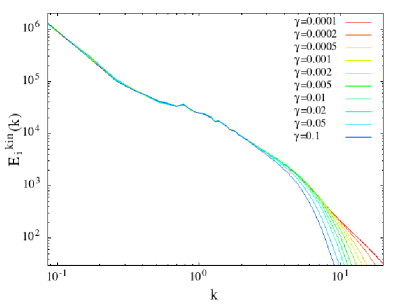
Figure 4 shows incompressible kinetic energy spectra (definition given in Sec. III) of the steady turbulent state for various values of . The energy spectra rapidly decays on the small scale () depending on the value of , while is not dependent on the value of at larger scales (). This indicates that the energy dissipation only occurs on the small scale and does not affect the large scale. In the main text, is adopted.
The dissipation term mimics the viscous term in the classical Navier-Stokes equation. To describe this, for simplicity, let us consider the single-component GP equation,
| (14) |
Using the Madelung transformation , the real part of Eq. (14) becomes
| (15) |
where and . Assuming that the density is almost uniform, the first term is dominant in the square bracket, which has the same form as the viscous term in the Navier-Stokes equation with a kinematic viscosity .
II Normalization of the Gross-Pitaevskii equation
The Gross-Pitaevskii (GP) equation that we solve has the form,
| (16) | |||||
where and . The nondimensional quantities are introduced as , , and , where and are the unit length and density, respectively. Substituting these into the GP equation, we obtain
| (17) | |||||
where , , , , and .
Here, the length unit is taken to be the interface width , and we have and . In the main text, the tildes in the nondimensional quantities are omitted, except .
III Kinetic energy spectra
In a manner similar to the single-component case, we consider the kinetic energy of the mass current as
| (18) |
where is the density per atom and is the velocity field of the mass current. In Eq. (18), the Fourier component is defined as . The kinetic energy can be decomposed into compressible and incompressible parts as
| (19) |
where and . The compressible and incompressible kinetic energy spectra are defined by
| (20) |
where and are the polar and azimuthal angles in wave-number space, respectively.
Figure 5 shows the energy spectra for the steady turbulent state for and various values of the Mach number , where the time average is taken for two stirring periods after steady turbulence is achieved. The raw data for are shown in Fig. 5(a), where lines with different deviate from each other. Since is predicted by the theory of Kolmogorov turbulence, we plot in Fig. 5(b), where the lines still deviate from each other, particularly around the “bump” (). We next rescale the length by the domain size , which is shown in Fig. 5(c). Since has dimensions of length to the power of , it should be divided by in this rescaling, which corresponds to the shift of the curves in Fig. 5(b) along the straight line . We find from Fig. 5(c) that the rescaled plots seem to collapse into a single universal curve, which follows a power law for and has a “bump” at .
The behavior in Fig. 5(c) can be interpreted as follows. The scale of corresponds to the inertial range, in which the incompressible kinetic energy cascades into smaller scales. In the inertial range, the “fluid” consists of many domains, and the movements of the domains produce vorticity distributions, as shown in Figs. 2(b) and 2(e) in the main text, which cascade into smaller scales. This energy cascade stops at the scale of the domain size (), since each domain itself does not contain quantized vortices and the vorticity cannot cascade into a scale smaller than the domain size. Thus, the inertial range terminates at , and a “bump” emerges in the energy spectrum for larger . This situation is similar to the quantum turbulence in a single-component superfluid, where a similar bump emerges at the scale of the mean distance between quantized vortices [15]. Below this scale, Kelvin-wave cascade occurs in the single-component case. In the present case, some excitation of domains may cause the energy to cascade into smaller scales, which merits further study. In Fig. 5(d), the energy spectra are further compensated by , which indicates that the Kolmogorov constant is almost unity.
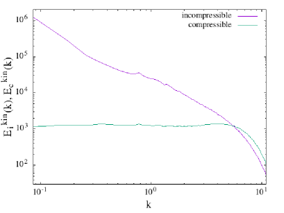
Figure 6 compares the kinetic energy spectra of the compressible and incompressible velocity fields. The compressible energy spectrum is much smaller than the incompressible energy spectrum for all scales, except the very small scale, which ensures that the incompressible dynamics are dominant in the inertial range of Kolmogorov turbulence.