GW170817 and GW190814: tension on the maximum mass

Abstract

The detection of the binary events GW170817 and GW190814 has provided invaluable constraints on the maximum mass of nonrotating configurations of neutron stars, $M_{{}_{\rm TOV}}$. However, the large differences in the neutron-star masses measured in GW170817 and GW190814 has also lead to a significant tension between the predictions for such maximum masses, with GW170817 suggesting that $M_{{}_{\rm TOV}}\lesssim 2.3\,M_{\odot}$, and GW190814 requiring $M_{{}_{\rm TOV}}\gtrsim 2.5\,M_{\odot}$ if the secondary was a (non- or slowly rotating) neutron star at merger. Using a genetic algorithm, we sample the multidimensional space of parameters spanned by gravitational-wave and astronomical observations associated with GW170817. Consistent with previous estimates, we find that all of the physical quantities are in agreement with the observations if the maximum mass is in the range $M_{{}_{\rm TOV}}=2.210^{+0.116}_{-0.123}\,M_{\odot}$ within a $2\textrm{-}\sigma$ confidence level. By contrast, maximum masses with $M_{{}_{\rm TOV}}\gtrsim 2.5\,M_{\odot}$, not only require efficiencies in the gravitational-wave emission that are well above the numerical-relativity estimates, but they also lead to a significant under-production of the ejected mass. Hence, the tension can be released by assuming that the secondary in GW190814 was a black hole at merger, although it could have been a rotating neutron star before.

1 Introduction

The recent detection of the gravitational-wave (GW) event GW190814 has seen involved the merger of black hole (BH), with a mass of $22.2-24.3\,M_{\odot}$, with a compact object having a much smaller mass of $2.50-2.67\,M_{\odot}$ (The LIGO Scientific Collaboration et al., 2020). The unclear nature of the secondary component has raised questions about the astrophysical evolutionary paths that would yield objects with these masses in a binary system. When assigning a NS nature to the secondary in GW190814, two scenarios are possible. In the first one, the secondary was a nonrotating or slowly rotating NS at merger, so that GW190814 should effectively be considered a BH-NS merger (see, e.g.,  Zevin et al., 2020; Safarzadeh et al., 2020; Kinugawa et al., 2020; Liu & Lai, 2020; Lu et al., 2020; Ertl et al., 2020, for some possible formation scenarios). In this case, the maximum mass $M_{{}_{\rm TOV}}$ of nonrotating NSs needs to reach values as large as $\gtrsim 2.5\,M_{\odot}$ (Fattoyev et al., 2020; Sedrakian et al., 2020; Tan et al., 2020; Tsokaros et al., 2020; Godzieba et al., 2020; Biswas et al., 2020). In the second scenario, the need for a large maximum mass can be replaced by the presence of rapid rotation. In fact, it has been shown that uniformly rotating NS can support about $20\%$ more mass than nonspinning ones (Breu & Rezzolla, 2016; Shao et al., 2020). Note that in the case of NSs with a phase transition, universal relations are still present, but depend on the properties of the phase transition (Bozzola et al., 2019; Demircik et al., 2020).

Based on these universal relations, Most et al. (2020b) and Zhang & Li (2020) have pointed out that a massive (rapidly) rotating NS with a mass $>2.5\,M_{\odot}$ is perfectly consistent with a maximum mass $M_{{}_{\rm TOV}}\simeq 2.3\,M_{\odot}$ inferred from the GW170817 event (see, e.g.,  Rezzolla et al., 2018; Shibata et al., 2019). Given the difficulty of sustaining rapid rotation over the very long timescales associated with the inspiral of the binary, the secondary must have collapsed at one point before merger, so that in this second scenario GW190814 should effectively be considered a BH-BH merger.

While a priori both scenarios are plausible, shedding light on which of them is the most likely is important from several points of view. To this scope, we here exploit the rich variety of GW and electromagnetic observables that have been obtained with GW170817 to explore the two scenarios combining the constraints set from the GW and electromagnetic signal from GW170817. In particular, we employ a genetic algorithm to sample through the distributions of maximum masses, ejected matter (Drout et al., 2017; Cowperthwaite et al., 2017; Kasen et al., 2017; Villar et al., 2017; Coughlin et al., 2018), and GW emission from numerical-relativity (NR) simulations (Zappa et al., 2018). Consistent with previous results (Rezzolla et al., 2018; Shibata et al., 2019) we find that GW170817’s observations clearly set an upper limit for the maximum mass of $M_{{}_{\rm TOV}}\lesssim 2.33\,M_{\odot}$. When forcing the algorithm to allow for maximum masses $M_{{}_{\rm TOV}}\gtrsim 2.4\,M_{\odot}$, we find that this requires unrealistically large GW efficiencies from the merger remnant and a deficit in the ejected matter.

2 Framework for the genetic algorithm

The observations of a bright blue kilonova has provided convincing evidence that the merger remnant in GW170817 could not have collapsed promptly to a BH. Rather, it must have survived for a timescale of the order of one second (Gill et al., 2019; Lazzati et al., 2020; Hamidani et al., 2020), and sufficiently large so that the hypermassive NS (HMNS) produced by the merger has reached uniform rotation at least in its core (Margalit & Metzger, 2017; Rezzolla et al., 2018). Following Rezzolla et al. (2018), we recall that quasi-universal relations exist between the masses of uniformly rotating stellar models along the stability line to BH formation and the corresponding dimensionless angular momentum $j_{\rm coll}$ normalised to the maximum (Keplerian) one $j_{\rm Kep}$ (Breu & Rezzolla, 2016). We here express this relation as

$$\chi(j_{\rm coll}/j_{\rm Kep}):=\frac{M_{\rm crit}}{M_{{}_{\rm TOV}}}=1+\alpha_{2}\left(\frac{j_{\rm coll}}{j_{\rm Kep}}\right)^{2}+\alpha_{4}\left(\frac{j_{\rm coll}}{j_{\rm Kep}}\right)^{4}\,,$$ (1)

where $\alpha_{2}=1.316\times 10^{-1}$ and $\alpha_{4}=7.111\times 10^{-2}$, and the value of the Keplerian specific angular momentum is approximately given by $j_{\rm Kep}\sim 0.68$ (see Eq. (4) in Most et al., 2020b, for more accurate estimates). The function $\chi$ is defined between 0 and 1 and describes all models with a mass that is critical for collapse to a BH. To fix ideas, in the case of nonorotating models, $j_{\rm coll}=0$ and $\chi(0)=1$, while for maximally rotating models $j_{\rm coll}=j_{\rm Kep}$ and (Breu & Rezzolla, 2016) $\chi(1):={M_{\rm max}}/{M_{{}_{\rm TOV}}}\approx 1.20_{-0.05}^{+0.02}$, where $M_{\rm max}$ is the maximum mass that can be sustained through uniform rotation (see Weih et al., 2018, for differentially rotating stars). Note that range $\chi(1)$ is based on a specific set of hadronic equations of state (EOSs) and that a different estimate suggests $\chi(1)=1.17_{-0.05}^{+0.02}$ (Shao et al., 2020).

Because Eq. (1) expresses a relation between gravitational masses, while the electromagnetic emission from GW170817 informs us about the ejected baryonic mass, we need a relation between gravitational and baryonic mass $M_{b}$ for uniformly rotating NSs at the mass-shedding limit (see, e.g.,  Timmes et al., 1996; Gao et al., 2020, for a detailed discussion). Also in this case, this relation obeys a quasi-universal relation near the values of the maximum mass that, with a $2\textrm{-}\sigma$ uncertainty, is given by $\eta:={M_{b,{\rm max}}}/{M_{\rm max}}\approx 1.171\pm 0.014$ at the maximum-mass limit (Rezzolla et al., 2018). Note that $\eta$ is in principle a function of $M$ and that the value reported above is for $M=M_{\rm max}$. However, $\eta$ is almost constant in the neighbourhood of $M_{\rm max}$ – where all of our considerations are made – so that hereafter we simply write the conversion between the two masses as $M_{b}=\eta M$.

The total gravitational mass of GW170817 as inferred from the GW signal is $M_{g}=2.73_{-0.01}^{+0.04}$ (The LIGO Scientific Collaboration et al., 2019), whose corresponding baryonic mass $M_{b}$ soon after the merger can be thought of as being given by the combination of the baryonic mass in the HMNS $M_{b,{{}_{\rm HMNS}}}$ – itself composed of the mass in the core and in a Keplerian disk – and of the mass ejected dynamically, i.e.,

$$M_{b}=M_{b,{\rm core}}+M_{b,{\rm disk}}+M_{\rm ej}^{\rm dyn}=\eta M^{*}_{g}\,,$$ (2)

where $M^{*}_{g}:=M_{g}-M_{\rm GW}^{\rm insp}$ and $M_{\rm GW}^{\rm insp}$ is the energy lost to GWs in the inspiral. Here, the last equality relates the baryonic and gravitational mass of the merger remnant. Defining now $\xi$ as the fraction of the HMNS baryonic mass in the core, the two components of the HMNS shortly after merger can be written as

$$M_{b,{\rm core}}:=\xi\left(M_{b}-M_{\rm ej}^{\rm dyn}\right)=\xi\left(\eta M^{*}_{g}-M_{\rm ej}^{\rm dyn}\right)$$ (3)

The fraction $\xi$ is in principle unknown, but numerical simulations have shown that this ratio is actually weakly dependent on the EOS and given by $\xi\approx 0.95^{+0.04}_{-0.05}$ (Hanauske et al., 2017). As time goes by, the merger remnant will loose part of its baryonic mass via the emission of magnetically driven or viscous-driven winds, so that at collapse it will have a baryonic mass

$$M_{b}=M_{b,{\rm core}}^{\rm coll}+M_{b,{\rm disk}}^{\rm coll}+M_{\rm ej}^{\rm dyn}+M_{\rm ej}^{\rm blue}+M_{\rm ej}^{\rm red}\,,$$ (4)

where the last equality follows from rest mass conservation and $M_{b,{\rm core}}^{\rm coll}$ and $M_{b,{\rm disk}}^{\rm coll}$ are the respective values of the core and the disk at the time when BH formation of the core is triggered, while $M_{\rm ej}^{\rm blue}$ ($M_{\rm ej}^{\rm red}$) is the part of the ejected matter leading to the blue (red) emission in the kilonova and differs from the dynamical ejecta from the timescale over which the material is lost. The two components also differ in the typical velocities of the matter, which is larger in the blue component ($v/c\lesssim 0.3$ for the blue part and $v/c\ll 0.1$ for the red part), but also with in the electron fraction $Y_{e}$, which is again larger in the blue component ($0.2\lesssim Y_{e}\lesssim 0.3$ for the blue part and $Y_{e}\lesssim 0.2$ for the red part). Numerical simulations of remnant disks indicate that most of the red ejecta originate from the disk, whereas most of the blue ejecta will come from the hot surface of the HMNS. Hence, for simplicity we will assume that the blue ejecta originate from the HMNS only, while the red ejecta exclusively represent unbound material of the disk. We classify the latter via a parameter

$$f_{\rm disk}:=M_{\rm ej}^{\rm red}/M_{b,{\rm disk}}\simeq 0.2-0.5\,,$$ (5)

representing the unbound fraction of the disk mass, which can be estimated based on numerical simulations (Siegel & Metzger, 2017; Fernández et al., 2019; Fujibayashi et al., 2018; Nathanail et al., 2020). In a merger scenario as that of GW170817, where the remnant may have lived for about one second (Gill et al., 2019), BH formation is triggered when the gravitational mass is reduced by the emission of GWs and the remnant hits the stability line for uniformly rotating models with a massive core $M_{b,\rm core}^{\rm coll}$

$$M_{b,\rm core}^{\rm coll} =\eta M^{*}_{g}-M_{b,{\rm disk}}-M_{\rm ej}^{\rm dyn}-M_{\rm ej}^{\rm blue}=\eta\chi M_{{}_{\rm TOV}}\,,$$ (6)

where the last equality relates the baryon mass of the remnant core to the maximum mass $M_{{}_{\rm TOV}}$ of nonrotating NS via Eq. (1). Indeed, when expressed as as a constraint equation on the maximum mass, Eq. (6) can also be written

$$\eta\chi M_{{}_{\rm TOV}}=\xi\left(\eta M^{*}_{g}-M_{\rm ej}^{\rm dyn}\right)-M_{\rm ej}^{\rm blue}\,.$$ (7)

Two more equations can be used for consistency

$$M_{\rm ej}^{\rm red} =f_{\rm disk}\left(1-\xi\right)\left(\eta M^{*}_{g}-M_{\rm ej}^{\rm dyn}\right)\,,$$ (8)

$$\chi M_{{}_{\rm TOV}} =M^{*}_{g}-\eta^{-1}\!\left(M_{b,{\rm disk}}^{\rm coll}\!+\!M_{\rm ej}^{\rm dyn}\!+\!M_{\rm ej}^{\rm blue}\!+\!M_{\rm ej}^{\rm red}\right)-M^{\rm post}_{{}_{\rm GW}}\,,$$ (9)

where the first one expresses the conservation of rest-mass leading to the kilonova emission and the second one the conservation of gravitational mass since $M^{\rm post}_{{}_{\rm GW}}$ is the mass lost to GWs after the merger. Expression (9) does not constrain $M^{\rm post}_{{}_{\rm GW}}$, which thus remains undetermined. As a way around (see also Fan et al. (2020)), we use an approximate quasi-universal relation between the total mass lost to GWs $M_{\rm GW}^{\rm tot}$ and the specific angular momentum of the remnant after the merger (Zappa et al., 2018)

$$m_{\rm GW}^{\rm tot}\sim c_{0}+c_{1}j_{\rm rem,20}+c_{2}\left(j_{\rm rem,20}\right)^{2}\,,$$ (10)

where $m_{\rm GW}^{\rm tot}:=M_{\rm GW}^{\rm tot}/({M_{g}\nu})$, $j_{\rm rem,20}:=J_{\rm rem,20}/(M_{g}^{2}\nu)$ is the specific angular momentum of the remnant within $\sim 20\,{\rm ms}$ from the merger, and $\nu:=m_{1}m_{2}/(m_{1}+m_{2})^{2}$ is the symmetric mass ratio. Note that $c_{0}=0.9,c_{1}=-0.4$ and $c_{2}=0.05$ (Zappa et al., 2018) and that the two component masses $m_{1}$ and $m_{2}$ are chosen considering the low-spin prior for GW170817, i.e., $\nu\in[0.243,0.25]$. By splitting total mass lost to GWs into the two components relative to the inspiral and post-merger, i.e., $M_{\rm GW}^{\rm tot}=M^{\rm insp}_{{}_{\rm GW}}+M^{\rm post}_{{}_{\rm GW}}$, Eq. (10) allows us to introduce an additional constraint between $j_{\rm coll}$ – which we derive from Eq. (1) – and $M^{\rm post}_{{}_{\rm GW}}$.

Two more remarks before concluding the presentation of our methodology. First, not all of the merger remnant’s angular momentum will end up in the collapsed object. A number of physical processes will move part of the angular momentum outwards, placing it on stable orbits relative to the newly formed BH. Because the efficiency of this process depends on microphysics that is poorly understood, we account for this by introducing a fudge factor $f_{B}$ defined as $j_{\rm coll}=:(1-f_{B})j_{\rm rem,20}$, so that the specific angular momentum of the disk is $j_{\rm disk}:=f_{B}j_{\rm rem,20}$. Second, since in Eqs. (7), (8) and (9) the function $\chi$ always appears together with $M_{{}_{\rm TOV}}$, it is difficult to set reasonable ranges for $\chi$. However, numerical simulations have revealed that the dimensionless spin of the BH produced by the merger $j_{{}_{\rm BH}}$ (and hence $j_{\rm coll}\lesssim j_{{}_{\rm BH}}$) is actually constrained in a rather limited range, i.e., $0.7\lesssim j_{{}_{\rm BH}}\lesssim 0.9$ (Kastaun et al., 2013; Bernuzzi et al., 2014). Exploiting this information, and assuming conservatively that $80\%$ of the specific angular momentum at collapse is inherited by the BH, i.e., $j_{\rm coll}=0.8\,j_{{}_{\rm BH}}$, we can effectively constrain $\chi$ to be in the range $1.11\leq\chi\lesssim 1.22$. Very similar results are obtained when making the more drastic assumption that only half of the BH spin comes from the remnant, i.e., $j_{\rm coll}=0.5\,j_{{}_{\rm BH}}$, which further reduces the lower limit to be $\chi=1.05$ (see Supplement Material for details).

In summary, we need to solve a multidimensional parametric problem as expressed by Eqs. (7), (8) and (9) after varying in the appropriate ranges the (ten) free parameters in the system: $\chi,\xi,\eta,M_{{}_{\rm GW}}^{\rm insp},M_{\rm ej}^{\rm blue},M_{\rm ej}^{\rm dyn},M_{{}_{\rm TOV}},\nu,f_{\rm disk}$ and $f_{B}$. While we treat all these parameters equally, some of them ($\eta,M_{\rm ej}^{\rm dyn},\nu$), vary in very narrow ranges and their variations do not significantly affect the overall results. In practice, at any iteration of the genetic algorithm we ensure that: (i) the total gravitational mass of the system is $M_{g}=2.73_{-0.01}^{+0.04}$ (The LIGO Scientific Collaboration & The Virgo Collaboration, 2017; The LIGO Scientific Collaboration et al., 2019); (ii) the total ejected mass is $M_{\rm ej}^{\rm tot}=0.0537\,\pm\,0.013\,M_{\odot}$ (Arcavi et al., 2017; Nicholl et al., 2017; Chornock et al., 2017; Cowperthwaite et al., 2017; Villar et al., 2017; Drout et al., 2017; Kasen et al., 2017; Tanaka et al., 2017; Waxman et al., 2018; Coughlin et al., 2018); (iii) the dynamically ejected mass is $M_{\rm ej}^{\rm dyn}\approx 10^{-3}\,M_{\odot}$ (Sekiguchi et al., 2015; Bovard et al., 2017; Radice et al., 2018; Poudel et al., 2020); (iv) the blue/red ejected components are respectively $0.005<M_{\rm ej}^{\rm blue}/M_{\odot}<0.02$ and $0.03<M_{\rm ej}^{\rm red}/M_{\odot}<0.55$ (Drout et al., 2017; Cowperthwaite et al., 2017; Smartt & Chen, 2017; Kasliwal et al., 2017; Kasen et al., 2017; Villar et al., 2017; Tanaka et al., 2017; Waxman et al., 2018; Coughlin et al., 2018) we have also explored a larger upper bound on the blue ejecta, i.e., $M_{\rm ej}^{\rm blue}/M_{\odot}<0.05$, finding no significant difference; see Supplemental Material; (v) the maximum mass is taken to be in the range $1.70\,M_{\odot}<M_{{}_{\rm TOV}}<3\,M_{\odot}$, note that the posterior lower bound is consistent with pulsar observations (Antoniadis et al., 2013; Cromartie et al., 2020); (vi) the energy radiated in GWs before the merger is constrained to be $0.035\lesssim M_{{}_{\rm GW}}^{\rm insp}/M_{\odot}\lesssim 0.045$ (Zappa et al., 2018). Note that all of the priors discussed in points (i)–(vi) are uniform.

3 Results

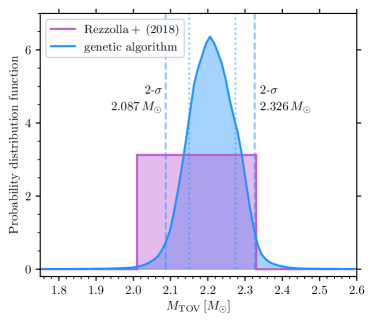
Figure 1: Uniform posterior from the analysis of Rezzolla et al. (2018) (magenta) and the posterior obtained with the multidimensional genetic algorithm (blue) discussed here. Indicated with vertical lines are the $1\textrm{-}\sigma$ (dotted) and $2\textrm{-}\sigma$ (dashed) values.

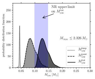
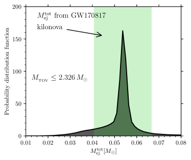
Figure 2: Left panel: Posteriors for the mass radiated in GWs consistent with the distribution in Fig. 1; the lavender-shaded area reports the upper limit coming from NR simulations. Right panel: Posterior for the total ejected mass consistent with the distribution in Fig. 1; the green-shaded area reports the range estimated in the literature.

Figure 1 provides a first important impression of the results of the genetic-algorithm. In particular, shown with a magenta-shaded area is the maximum-mass estimate made by Rezzolla et al. (2018) and which is a simple uniform posterior for $M_{{}_{\rm TOV}}=2.16_{-0.16}^{+0.17}\,M_{\odot}$. Shown instead with a blue-shaded area is the posterior distribution obtained with the genetic algorithm. The median of the distribution is $M_{{}_{\rm TOV}}=2.210^{+0.117}_{-0.123}\,M_{\odot}$, where the errors reported here are for $2\textrm{-}\sigma$ uncertainty. Overall, this yields a lower bound of $M_{{}_{\rm TOV}}>2.087\,M_{\odot}$ and an upper bound of $M_{{}_{\rm TOV}}<2.326\,M_{\odot}$ at $2\textrm{-}\sigma$ level (vertical dashed lines), and thus in good agreement with massive-pulsar measurements (Antoniadis et al., 2013; Cromartie et al., 2020) and previous estimates (Rezzolla et al., 2018; Shibata et al., 2019). Interestingly, our results are in good agreement with the conclusions reached by Shao et al. (2020) and Fan et al. (2020), who have also considered the post-merger GW emission to deduce bounds on the maximum mass.

As a consistency check, we can use set of parameters that yield the maximum-mass distribution in Fig. 1, to estimate the GW energy lost both in the inspiral and in the post-merger. This is shown in the left panel of Fig. 2, where we report the posterior distributions for $M_{{}_{\rm GW}}^{\rm insp}$ (black dotted line) and $M_{\rm GW}^{\rm post}$ (black dashed line), as well as their sum, $M_{{}_{\rm GW}}^{\rm tot}$ (black solid line). Also marked with a vertical lavender-shaded is the upper limit estimated by Zappa et al. (2018), $E^{\rm tot}_{\rm GW}/M_{g}\leq 0.045\,M_{\odot}c^{2}$, on the basis of a large number of NR simulations, with an associated uncertainty of $20\%$. A similar consistency is found in the right panel of Fig. 2, where we report the posterior of the total ejected mass consistent with the maximum-mass distribution in Fig. 1. Indicated with a green-shaded area are the constraints obtained from the kilonova observations of GW170817. More specifically, the width of the shaded area represents the standard deviation using various estimates for the total ejected mass $M_{\rm ej}^{\rm tot}$ estimated for GW170817 (Arcavi et al., 2017; Nicholl et al., 2017; Chornock et al., 2017; Cowperthwaite et al., 2017; Villar et al., 2017; Drout et al., 2017; Kasen et al., 2017; Tanaka et al., 2017; Waxman et al., 2018; Coughlin et al., 2018). Clearly, also the ejected-mass distribution is in perfect agreement with observational bounds when the maximum mass is below $2.326\,M_{\odot}$.

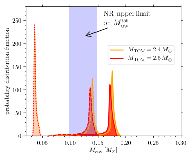
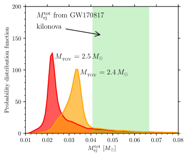
Figure 3: Left panel: The same as in the left panel of Fig. 2, but when considering two fixed values for the maximum mass, i.e., $M_{{}_{\rm TOV}}=2.4\,M_{\odot}$ (orange) and $M_{{}_{\rm TOV}}=2.5\,M_{\odot}$ (red). Right panel: The same as in the right panel of Fig. 2, but for two fixed maximum-mass values.

Given these results, it is natural to ask: does anything break down when larger maximum masses are considered? The positive answer to this question is contained in Fig. 3, whose panels are similar to those in Fig. 2, when however the genetic algorithm is forced to consider two specific values of the maximum mass, namely, $M_{{}_{\rm TOV}}=2.4\,M_{\odot}$ and $M_{{}_{\rm TOV}}=2.5\,M_{\odot}$. Concentrating first on the left panel of Fig. 3, it is clear that when allowing for large maximum masses, the mass radiated in GWs after the merger, $M_{{}_{\rm GW}}^{\rm post}$ (red dashed line), is significantly larger than what NR simulations predict; this is true both for $M_{{}_{\rm TOV}}=2.4\,M_{\odot}$ and for $M_{{}_{\rm TOV}}=2.5\,M_{\odot}$. This behaviour is due to the fact that remnants with a given $\chi$ will radiate more GWs if they are more massive [cf., Eq. (9)]. Next, when considering the right panel of Fig. 3 it is also easy to realize that large maximum masses lead to a deficit in the ejected matter. This is simply due to the fact that considering large-mass stars inevitably reduces the portion of the budget available for the ejecta. We have confirmed that, even if (unrealistically) large additional angular momentum transport was assumed, these results remain unchanged for $M_{{}_{\rm TOV}}\gtrsim 2.5\,M_{\odot}$, (see Supplemental Material).

In summary, while a value $M_{{}_{\rm TOV}}\lesssim 2.3\,M_{\odot}$ is fully consistent with the GW emission from NR simulations and the observed ejected mass, a value $M_{{}_{\rm TOV}}\gtrsim 2.5\,M_{\odot}$ requires efficiencies in the GW emission that are well above the estimates from a large number of accurate NR simulations and, overall, leads to an under-production of ejected mass.

4 Conclusions

We have carried out a systematic investigation to ascertain whether the tension on the maximum mass following the detections of GW170817 and GW190814 can in some way be resolved or at least attenuated. In particular, we have employed a genetic algorithm to sample through the multidimensional space of parameters that can be built on the basis of the astronomical observations (i.e., ejected mass in the various components), GW observations (i.e., gravitational masses of the binary components), and of NR simulations (i.e., properties of the remnant and efficiency of GW emission).

The results of this investigation have allowed us to refine in a probabilistic manner the previous estimates of the maximum mass (Rezzolla et al., 2018), obtaining that $M_{{}_{\rm TOV}}=2.210^{+0.117}_{-0.123}\,M_{\odot}$ within a $2\textrm{-}\sigma$ confidence level. In this range, all of the physical quantities are in very good agreement with the estimates coming from the observations. By contrast, we find that considering maximum masses with $M_{{}_{\rm TOV}}\gtrsim 2.4-2.5\,M_{\odot}$ requires efficiencies in the GW emission well above the NR estimates and leads to a significant under-production of the ejected mass, well below the values expected from the observations. Although robust, our results can be strengthened in a number of ways. Improved post-merger modeling and long-term NR simulations (Fujibayashi et al., 2018) can help to narrow the uncertainties in the parameter ranges for $\chi$ and $j_{\rm rem}$. Refined universal relations of uniformly rotating NSs including temperature dependence (Koliogiannis & Moustakidis, 2020), will also help narrowing down the errors in $\eta$ and the upper limit of $\chi$. Such improvements will be crucial to understand the viability of the maximum-mass constraint for $M_{\rm TOV}\lesssim 2.3\,M_{\odot}$.

In light of these considerations, we conclude that the secondary in GW190814 was most likely a BH at merger, although it may well have been a rotating NS at some stage during the evolution of the binary system.

Acknowledgements. It is a pleasure to thank C. Ecker, J. Papenfort, and L. Weih for useful comments. Support comes in part also from “PHAROS”, COST Action CA16214 and the LOEWE-Program in HIC for FAIR. ERM gratefully acknowledges support from a joint fellowship at the Princeton Center for Theoretical Science, the Princeton Gravity Initiative and the Institute for Advanced Study.

Supplemental Material

In what follows we provide additional information that complements the one provided in the main text. While the details illustrated below do not vary the conclusions drawn in the main text, they provide additional technical details on the genetic algorithm employed in our analysis. In addition, they help investigate how the results change when the parameters are varied beyond the (reasonable) ranges assumed so far.

For the solution of our multidimensional parametric problem the procedure we adopt is as follows (see also Fromm et al., 2019; Nathanail et al., 2020, for additional information). We start by recalling that genetic algorithms are designed to generate high-quality solutions to problems of this type where a searching optimization is sought. The name follows from the operators of mutation, crossover and selection that are normally found in biological systems. Our choice of a genetic algorithm in place of a more traditional Bayesian analysis based on a Markov-Chain Monte Carlo approach is motivated mostly by the overall simplicity of our problem and the reduced computational costs that are associated with a genetic algorithm.

In practice, our algorithm samples through the parameter space of the ten free parameters. From those it computes the $M_{\rm ej}^{\rm red}$ through Eqs. (3) and (5), $M^{\rm post}_{{}_{\rm GW}}$ through Eq. (10) and the specific angular momentum at collapse $j_{\rm coll}$ via Eq. (1), using the sampled value of$\chi$. Subsequently, Eqs. (7), (8), and (9) are solved to match the observed values of $M_{g}$ and $M_{\rm ej}^{\rm tot}$ within the errors, finding the best-fit values. The genetic algorithm employed here makes use of Python packages from the SciPY software library (Virtanen et al., 2020).

As a corollary to the discussion made in the main text and relative to Figs. 1–3, we provide with the corner plots in Fig. 4 information on the probability distribution functions of the various quantities involved in our analysis. More specifically, Fig. 4 shows the corner plot relative to maximum-mass posterior shown in Fig. 1 and should therefore accompany the information presented in Fig. 2. On the other hand, Fig. 5 refers to the case when the genetic algorithm is forced to consider $M_{{}_{\rm TOV}}=2.5\,M_{\odot}$. In this case, the maximum-mass is set to vary uniformly in the very small interval around $M_{{}_{\rm TOV}}=2.5^{+0.0001}_{-0.0001}\,M_{\odot}$, leaving all the other parameters free to be adjusted till a best-fit is found. In this sense, the information in Fig. 5 complements what is reported in Fig. 3 and shows that all the posterior distributions are pushed to be very narrow at the edges of the allowed ranges. For instance, the dimensionless spin $\chi$ is narrowly peaked around its minimum value $1.1$, the mass in the disk is much smaller and of the order of $\simeq 0.035\,M_{\odot}$, while the blue and red ejecta are comparable and equal to $\simeq 0.019\,M_{\odot}$.

Note that to avoid having a large number of small panels, we have limited ourselves either to the most salient ones, omitting those quantities for which the distributions are either almost constant or restricted to a very small region. More specifically, in Fig. 4 the values found are: $\xi=0.973_{-0.035}^{+0.011}$, $\eta=1.171_{-0.013}^{+0.014}$, $M_{\rm ej}^{\rm dyn}=0.001_{-0.001}^{+0.001}\,M_{\odot}$, $f_{\rm disk}=0.437_{-0.209}^{+0.061}$, and $\nu=0.243_{-0.000}^{+0.005}$, which corresponds to $q=0.719_{-0.006}^{+0.136}$. We have also explored a modified scenario in which the blue ejecta are larger than inferred from observations. In particular, we have adjusted the upper bound on the blue ejecta from $M_{\rm ej}^{\rm blue}/M_{\odot}<0.02$ to $M_{\rm ej}^{\rm blue}/M_{\odot}<0.05$. In this case, we find that the blue ejecta converge to a distribution with a median around $\sim 0.03\,M_{\odot}$, while the red ejecta component decreases to $\sim 0.02\,M_{\odot}$. At the same time, the changes in the posterior for the maximum mass are minute, i.e., $M_{{}_{\rm TOV}}=2.192^{+0.125}_{-0.092}\,M_{\odot}$.

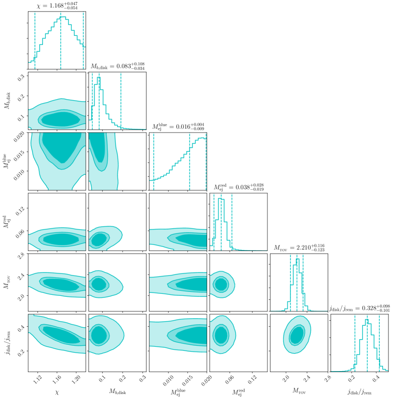
Figure 4: Corner plot reporting the posterior distributions of the most important parameters in our analysis. Indicated with the two outermost vertical dashed lines are the corresponding $2\textrm{-}\sigma$ values, while the labels on the diagonal cells report the average values (central vertical dashed line).

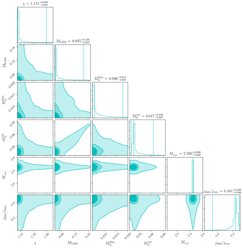
Figure 5: Same as Fig. 4 but when the maximum mass is held fixed at the value $M_{{}_{\rm TOV}}=2.5\,M_{\odot}$.

Finally, in Fig. 6 we provide information that is similar in content to that in Fig. 3, but when we allow for the dimensionless spin to attain even smaller values, i.e., $1.05\leq\chi\lesssim 1.22$. Note that in this case, the ejected mass for $M_{{}_{\rm TOV}}=2.4\,M_{\odot}$ is within the observational bounds, but the excess in radiated mass is more severe. The disagreement becomes even stronger for $M_{{}_{\rm TOV}}=2.5\,M_{\odot}$.

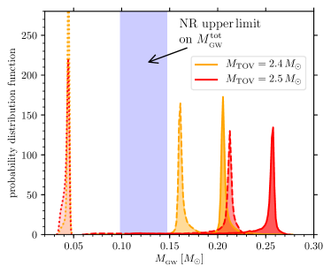
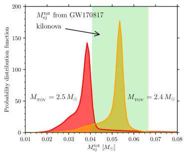
Figure 6: The same as Fig. 3 but when we allow for the dimensionless spin to attain even smaller values, i.e., $1.05\leq\chi\lesssim 1.22$. Note that in this case disagreement in the radiated and ejected mass becomes even stronger for $M_{{}_{\rm TOV}}=2.5\,M_{\odot}$.

As a concluding remark we note that the interpretation of the nature of GW190425 is likely unaffected by our findings on the maximum masses of neutron stars. While a BH-NS nature cannot be fully ruled out, the most plausible case of a NS-NS nature of the system is perfectly compatible with our findings on the maximum mass, as the initial masses in GW190425 are both well below the maximum-mass limit we have presented here (see also Most et al., 2020a, for a discussion on GW190425). On the other hand, an indirect impact that our results have on GW190425 is on whether the merger led to a prompt collapse (i.e., where the hypermassive neutron star collapses to a black hole either at or shortly after merger), or to a stable long lived remnant. Using the results of Koeppel et al. (2019) (but see also Bauswein et al., 2017), and given the values for the maximum mass found here, a prompt or delayed collapse scenario seems likely for GW190425.

References

- Antoniadis et al. (2013) Antoniadis, J., Freire, P. C. C., Wex, N., et al. 2013, Science, 340, 448
- Arcavi et al. (2017) Arcavi, I., Hosseinzadeh, G., Howell, D. A., et al. 2017, Nature, 551, 64
- Bauswein et al. (2017) Bauswein, A., Just, O., Janka, H.-T., & Stergioulas, N. 2017, Astrophys. J. Lett., 850, L34
- Bernuzzi et al. (2014) Bernuzzi, S., Dietrich, T., Tichy, W., & Brügmann, B. 2014, Phys. Rev. D, 89, 104021
- Biswas et al. (2020) Biswas, B., Nandi, R., Char, P., Bose, S., & Stergioulas, N. 2020, arXiv e-prints, arXiv:2010.02090
- Bovard et al. (2017) Bovard, L., Martin, D., Guercilena, F., et al. 2017, Phys. Rev. D, 96, 124005
- Bozzola et al. (2019) Bozzola, G., Espino, P. L., Lewin, C. D., & Paschalidis, V. 2019, European Physical Journal A, 55, 149
- Breu & Rezzolla (2016) Breu, C., & Rezzolla, L. 2016, Mon. Not. R. Astron. Soc., 459, 646
- Chornock et al. (2017) Chornock, R., Berger, E., Kasen, D., et al. 2017, Astrophys. J. Letters, 848, L19
- Coughlin et al. (2018) Coughlin, M. W., Dietrich, T., Doctor, Z., et al. 2018, Mon. Not. R. Astron. Soc., 480, 3871
- Cowperthwaite et al. (2017) Cowperthwaite, P. S., Berger, E., Villar, V. A., et al. 2017, Astrophys. J. Lett., 848, L17
- Cromartie et al. (2020) Cromartie, H. T., Fonseca, E., Ransom, S. M., et al. 2020, Nature Astronomy, 4, 72
- Demircik et al. (2020) Demircik, T., Ecker, C., & Järvinen, M. 2020, arXiv e-prints, arXiv:2009.10731
- Drout et al. (2017) Drout, M. R., Piro, A. L., Shappee, B. J., et al. 2017, Science, 358, 1570
- Ertl et al. (2020) Ertl, T., Woosley, S. E., Sukhbold, T., & Janka, H. T. 2020, Astrophys. J., 890, 51
- Fan et al. (2020) Fan, Y.-Z., Jiang, J.-L., Tang, S.-P., Jin, Z.-P., & Wei, D.-M. 2020, Astrophys. J., 904, 119
- Fattoyev et al. (2020) Fattoyev, F. J., Horowitz, C. J., Piekarewicz, J., & Reed, B. 2020, arXiv e-prints, arXiv:2007.03799
- Fernández et al. (2019) Fernández, R., Tchekhovskoy, A., Quataert, E., Foucart, F., & Kasen, D. 2019, Mon. Not. R. Astron. Soc., 482, 3373
- Foreman-Mackey (2016) Foreman-Mackey, D. 2016, Journal of Open Source Software, 1, 24
- Fromm et al. (2019) Fromm, C. M., Younsi, Z., Baczko, A., et al. 2019, Astron. Astrophys., 629, A4
- Fujibayashi et al. (2018) Fujibayashi, S., Kiuchi, K., Nishimura, N., Sekiguchi, Y., & Shibata, M. 2018, The Astrophysical Journal, 860, 64
- Gao et al. (2020) Gao, H., Ai, S.-K., Cao, Z.-J., et al. 2020, Frontiers of Physics, 15, 24603
- Gill et al. (2019) Gill, R., Nathanail, A., & Rezzolla, L. 2019, Astrophys. J., 876, 139
- Godzieba et al. (2020) Godzieba, D. A., Radice, D., & Bernuzzi, S. 2020, arXiv e-prints, arXiv:2007.10999
- Hamidani et al. (2020) Hamidani, H., Kiuchi, K., & Ioka, K. 2020, Mon. Not. R. Astron. Soc., 491, 3192
- Hanauske et al. (2017) Hanauske, M., Takami, K., Bovard, L., et al. 2017, Phys. Rev. D, 96, 043004
- Kasen et al. (2017) Kasen, D., Metzger, B., Barnes, J., Quataert, E., & Ramirez-Ruiz, E. 2017, Nature, 551, 80
- Kasliwal et al. (2017) Kasliwal, M. M., Nakar, E., Singer, L. P., et al. 2017, Science, 358, 1559
- Kastaun et al. (2013) Kastaun, W., Galeazzi, F., Alic, D., Rezzolla, L., & Font, J. A. 2013, Phys. Rev. D, 88, 021501
- Kinugawa et al. (2020) Kinugawa, T., Nakamura, T., & Nakano, H. 2020, arXiv e-prints, arXiv:2007.13343
- Koeppel et al. (2019) Koeppel, S., Bovard, L., & Rezzolla, L. 2019, Astrophys. J. Lett., 872, L16
- Koliogiannis & Moustakidis (2020) Koliogiannis, P. S., & Moustakidis, C. C. 2020, arXiv e-prints, arXiv:2007.10424
- Lazzati et al. (2020) Lazzati, D., Ciolfi, R., & Perna, R. 2020, Astrophys. J., 898, 59
- Liu & Lai (2020) Liu, B., & Lai, D. 2020, arXiv e-prints, arXiv:2009.10068
- Lu et al. (2020) Lu, W., Beniamini, P., & Bonnerot, C. 2020, arXiv e-prints, arXiv:2009.10082
- Margalit & Metzger (2017) Margalit, B., & Metzger, B. D. 2017, Astrophys. J. Lett., 850, L19
- Most et al. (2020a) Most, E. R., Papenfort, L. J., Tootle, S., & Rezzolla, L. 2020a, arXiv e-prints, arXiv:2012.03896
- Most et al. (2020b) Most, E. R., Papenfort, L. J., Weih, L. R., & Rezzolla, L. 2020b, Mon. Not. R. Astron. Soc., 499, L82
- Nathanail et al. (2020) Nathanail, A., Gill, R., Porth, O., Fromm, C. M., & Rezzolla, L. 2020, Mon. Not. R. Astron. Soc., 495, 3780
- Nicholl et al. (2017) Nicholl, M., Berger, E., Kasen, D., et al. 2017, Astrophys. J. Letters, 848, L18
- Poudel et al. (2020) Poudel, A., Tichy, W., Brügmann, B., & Dietrich, T. 2020, Phys. Rev. D, 102, 104014
- Radice et al. (2018) Radice, D., Perego, A., Hotokezaka, K., et al. 2018, Astrophys. J., 869, 130
- Rezzolla et al. (2018) Rezzolla, L., Most, E. R., & Weih, L. R. 2018, Astrophys. J. Lett., 852, L25
- Safarzadeh et al. (2020) Safarzadeh, M., Ramirez-Ruiz, E., & Berger, E. 2020, arXiv e-prints, arXiv:2001.04502
- Sedrakian et al. (2020) Sedrakian, A., Weber, F., & Li, J. J. 2020, Phys. Rev. D, 102, 041301
- Sekiguchi et al. (2015) Sekiguchi, Y., Kiuchi, K., Kyutoku, K., & Shibata, M. 2015, Phys. Rev. D, 91, 064059
- Shao et al. (2020) Shao, D.-S., Tang, S.-P., Sheng, X., et al. 2020, Phys. Rev. D, 101, 063029
- Shibata et al. (2019) Shibata, M., Zhou, E., Kiuchi, K., & Fujibayashi, S. 2019, Phys. Rev. D, 100, 023015
- Siegel & Metzger (2017) Siegel, D. M., & Metzger, B. D. 2017, Physical Review Letters, 119, 231102
- Smartt & Chen (2017) Smartt, S., & Chen, T. e. a. 2017, Nature, 551, 75
- Tan et al. (2020) Tan, H., Noronha-Hostler, J., & Yunes, N. 2020, arXiv e-prints, arXiv:2006.16296
- Tanaka et al. (2017) Tanaka, M., Utsumi, Y., Mazzali, P. A., et al. 2017, Public. Astron. Soc. of Japan, 69, 102
- The LIGO Scientific Collaboration & The Virgo Collaboration (2017) The LIGO Scientific Collaboration, & The Virgo Collaboration. 2017, Phys. Rev. Lett., 119, 161101
- The LIGO Scientific Collaboration et al. (2019) The LIGO Scientific Collaboration, the Virgo Collaboration, Abbott, B. P., et al. 2019, Physical Review X, 9, 011001
- The LIGO Scientific Collaboration et al. (2020) The LIGO Scientific Collaboration, the Virgo Collaboration, Abbott, R., et al. 2020, Astrophys. J. Lett., 896, L44
- Timmes et al. (1996) Timmes, F. X., Woosley, S. E., & Weaver, T. A. 1996, Astrophys. J., 457, 834
- Tsokaros et al. (2020) Tsokaros, A., Ruiz, M., & Shapiro, S. L. 2020, arXiv e-prints, arXiv:2007.05526
- Villar et al. (2017) Villar, V. A., Guillochon, J., Berger, E., et al. 2017, Astrophys. J. Letters, 851, L21
- Virtanen et al. (2020) Virtanen, P., Gommers, R., Oliphant, T. E., et al. 2020, Nature Methods, 17, 261
- Waxman et al. (2018) Waxman, E., Ofek, E., Kushnir, D., & Gal-Yam, A. 2018, Mon. Not. R. Astron. Soc., 481, 3423
- Weih et al. (2018) Weih, L. R., Most, E. R., & Rezzolla, L. 2018, Mon. Not. R. Astron. Soc., 473, L126
- Zappa et al. (2018) Zappa, F., Bernuzzi, S., Radice, D., Perego, A., & Dietrich, T. 2018, Physical Review Letters, 120, 111101
- Zevin et al. (2020) Zevin, M., Spera, M., Berry, C. P. L., & Kalogera, V. 2020, arXiv e-prints, arXiv:2006.14573
- Zhang & Li (2020) Zhang, N.-B., & Li, B.-A. 2020, Astrophys. J., 902, 38