Comprehensive broadband study of accreting neutron stars with Suzaku: Is there a bi-modality in the X-ray spectrum?

Abstract

We present a broadband spectral analysis of accreting neutron stars using data from XIS and PIN onboard Suzaku. From spectral fits of these sources with a single continuum model including a powerlaw and high energy cut-off, cyclotron lines (where required), we studied the correlation between various spectral parameters. Among 39 sources we studied, 16 are those where the existence of a cyclotron line is known in literature, and 29 need a cutoff energy. Among these 29 sources, 18 have cutoff energy bunched in a range of 3-10 keV while for 11 sources, it spreads over 12-25 keV. This bi-modal behaviour is not based on the specific nature of the systems being a Be XRB or supergiant HMXB, nor on different beaming patterns characterizing their X-ray emission (as inferred from simultaneous study of their pulse profiles). The broadband coverage of Suzaku also shows that the cutoff energies saturate for higher values of cyclotron line energies - consistent with previous works in literature - for both the groups and the width of the cyclotron line show a weak correlation with the cyclotron line energy. We also find an anticorrelation with luminosity for both spectral index and folding energy, respectively. Unlike previous works, we did not detect any anticorrelation between X-ray luminosity and EW of K$\alpha$ lines. Finally, we show that the EW and flux of the iron K$\alpha$ line are smaller in SFXTs than classical NS-HMXBs. We discuss these findings in terms of different properties of stellar winds and accretion mechanisms.

1 Introduction

High-mass X-ray binaries (HMXBs) are binary systems comprising a compact object and a massive star orbiting around a common centre of mass. The compact object can be either a neutron star or a black hole. In this work, we mainly deal with HMXBs that harbour a neutron star as the compact object accreting from the powerful wind of the massive companion (White, Swank & Holt, 1983; Nagase, 1989; Bildsten et al., 1997). These neutron stars in HMXBs have magnetic fields of the order of $\gtrsim$ 10¹² G. The accreted material is thus expected to be channelled along the magnetic field lines at relatively large distances from the compact object, leading to the formation of extended accretion columns. The exact details of how the magnetic field affects the accretion flow is still a topic of investigation (Becker & Wolff, 2007). It is generally expected that the inflowing material is directed towards the the magnetic poles of the neutron star where two hot spots are formed. The gravitational potential energy of the inflowing material is first converted into kinetic energy and then released as X-rays due to shocks and dissipations into the accretion column and on the hot spots (Basko & Sunyaev, 1975). If the rotation axis and the magnetic axis of the neutron star are not completely aligned, the X-ray emission from the source appears pulsed to any distant observer whose line of sight to the object intersects the beam periodically.
The high magnetic fields of neutron stars can be measured from the cyclotron resonance scattering features (CRSFs). These features are known to be produced as a consequence of cyclotron resonant scattering of X-ray photons in the presence of an intense magnetic field. Their centroid energy is related to the NS magnetic field intensity by the equation:

$$E_{\rm{C}}=11.6\frac{B}{10^{12}\,\rm{G}}(1+z)^{-1}\rm{\,keV},$$ (1)

where $z$ is the gravitational redshift.
Classical HMXBs can be classified as either Be/X-ray binaries (BeXBs; Reig 2011) or Supergiant X-ray binaries (SGXBs; Walter et al. 2015). Relatively recently discovered HMXBs with supergiant companions, called Supergiant Fast X-ray Transients (SFXTs), are characterized by short outbursts with fast rise times ($\sim$ tens of minutes) and typical durations of a few hours (Sguera et al., 2006). For this study, along with both classical HMXBs and SFXTs observed with Suzaku (Mitsuda et al., 2007), we have also included a few sources which have a low mass companion star but are known to harbour neutron star with strong magnetic fields. These four sources are Her X-1, 4U 1626-67, GX 1+4, and 4U 1822-37 and have been classified here as Low Mass X-ray Binaries, LMXBs (although strictly speaking, Her X-1 is an intermediate mass X-ray binary).

2 Data Reduction

Suzaku (Mitsuda et al., 2007) is a broad-band X-ray observatory covering the energy range 0.2-600 keV. There are two main instruments on-board Suzaku: the X-ray Imaging Spectrometer XIS (Koyama et al., 2007), covering the 0.2-12 keV energy range, and the Hard X-ray Detector (HXD). The XIS consists of four CCD detectors of which three (XIS 0, 2 and 3) are front illuminated (FI) and one (XIS 1) is back illuminated (BI). The HXD comprises PIN diodes (Takahashi et al., 2007) that cover the 10-70 keV energy range and GSO crystal scintillator detectors that cover the 70-600 keV energy range.
For the XIS and the HXD data, we used the filtered cleaned event files which are obtained using the pre-determined screening criteria as suggested in the Suzaku ABC guide. The data reduction for both instruments was carried out following the reduction technique mentioned in the same Suzaku ABC guide. We applied the barycentric correction to all event files using aepipeline. For the XIS data reduction we applied the following procedure: for sources that showed jitters in the image, the event files were corrected by using the aeattcorr and xiscoord tools to update the attitude information; for those sources affected by pile-up, we discarded photons collected within the portion of the PSF where the estimated pile-up fraction was greater than 4 %. This was done by using the FTOOLS task pileest. XIS spectra were then extracted by choosing circular regions of $2^{{}^{\prime}}$, $3^{{}^{\prime}}$, or $4^{{}^{\prime}}$ radius from the source position depending on whether the observation was made in 1/8, 1/4, or 0 window mode, respectively. Background spectra for the XIS were extracted by selecting regions of the same size as mentioned above in a portion of the CCD that was not significantly contaminated by the source X-ray emission. For relatively fainter objects observed in window ‘Off’ mode (like IGR J16493-4348, IGR J16465-4507, IGR J16479-4514, and IGR J08408-4503) choosing the same radius for the source and background extraction region gave rise to a dip-like artefact in the spectra visible around 6 keV. Hence, for these sources, a larger background region was chosen by adopting an annulus with inner (outer) radius of 5 ${}^{{}^{\prime}}$ (7 ${}^{{}^{\prime}}$) centered on the source best known position.
The PIN source spectra were additionally corrected for dead-time effects by using the FTOOLS task hxddtcor. For the HXD/PIN, simulated ‘tuned’ non X-ray background event files (NXB) corresponding to the month and year of the respective observations were used to estimate the non X-ray background (Fukazawa et al., 2009).
The XIS spectra were extracted with 2048 channels and the PIN spectra with 255 channels. Response files for the XIS were created using the CALDB version ‘20150312’. For the HXD/PIN spectrum, response files corresponding to the epoch of the observation were obtained from the Suzaku guest observer facility.
The sources considered for the present study and all the OBSID corresponding to the observations used are listed in Table LABEL:obslog.

3 Spectral Analysis

For the spectral analysis of the selected sources, we have used the spectra from all the available XIS units (0, 1, 2 and 3) and the PIN. In some cases we noticed systematic differences between the spectra obtained from the BI XIS 1 and the rest of the XIS units. In all these cases, we did not make use of the BI XIS 1 data in the spectral fitting as they gave no additional information and led to a poorer fit with larger $\chi^{2}_{\rm red}$. Spectral fitting was performed by using XSPEC v12.9.0. Artificial residuals are known to arise in the XIS spectra around the Si edge and the Au edge. We have thus discarded the energy range $\sim$ 1.7-2.3 keV for spectral analysis. For most sources, we have limited our analysis to the energy range $\sim$ 0.8-10.0 keV for XIS and 15.0-70.0 keV for the HXD-PIN. For sources like OAO 1657-415, 4U 1909+07, IGR J16393-4643, GX 301-2, and GX 1+4 where the absorption at soft X-ray is larger, we did not use data below $\sim$ 3 keV either due to the poor signal-to-noise ratio (S/N) or because the spectra below 3 keV show a ‘low energy tail’ which is not characteristic of the source but has an instrumental origin (Suchy et al., 2012). For other sources characterized by a PIN spectrum with limited statistics, like V 0332+53, 4U 1909+07, IGR J16393-4643, 4U 2206+54, SW J2000.6+3210, and 4U 1822-37, we have discarded the data points in the PIN spectrum, above the energy where the S/N is very low. For some sources like 4U 1907+09, 4U 1700-37, and IGR J17544-2619, we noticed an excess above the power-law continuum in the data around 10 keV, with an amplitude of 10 %, 10% and 5 % respectively. This ‘10 keV’ feature was also previously reported in the cases of 4U 1907+09 and 4U 1538-522 (Rivers et al., 2010; Coburn et al., 2002). Since the aim of this work is to perform a homogeneous fit as much as possible, we discarded in all cases the data around this feature.
For IGR J16318-4848, we limited our analysis to the energy range 5.0-60.0 keV, owing to very strong absorption below 5.0 keV and the low S/N above 60 keV (Barragán et al., 2009). For seven sources (IGR J16195-4945, IGR J16493-4348, IGR J16465-4507, IGR J16479-4514, IGR J17391-3021, IGR J08408-4503, and IGR J00370+6122), we could make use only of the XIS data as their PIN spectrum was contaminated either by nearby bright sources, or by the diffuse emission from Galactic Ridge, or due to the high CXB and NXB (Morris et al., 2009; Sidoli et al., 2013; Bodaghee et al., 2011; Sidoli, Esposito & Ducci, 2010). For eclipsing HMXBs like Her X-1, LMC X-4, Cen X-3, 4U 1700-37, 4U 1538-522, SMC X-1, Vela X-1, OAO 1657-415, 4U 1822-37, IGR J16479-4514 and IGR J16195-4945, we have checked whether the source was in eclipse or not during the considered observations by folding its lightcurve together with the corresponding RXTE-ASM orbital lightcurve at the known orbital period of the source. Except for Cen X-3, IGR J16479-4514, and 4U 1822-37, all the other sources were not observed during an X-ray eclipse. For Cen X-3 and IGR J16479-4514, we have extracted the time filtered spectrum corresponding to the times when the source was not in eclipse. For Cen X-3 we extracted spectra only for ‘Segment E’ of Naik, Paul & Ali (2011) while for IGR J16479-4514, we extracted the spectrum starting 143 ks after the beginning of the observation (as is done in Sidoli et al. 2013). For 4U 1822-37, the full Suzaku observation spanned nearly four times the orbital period of the neutron star. Hence for 4U 1822-37, we extracted a spectrum only for that phase interval during which the source was outside the dips and eclipse (0.1-0.6 when Phase 0 is at MJD 54010.48). In the cases of Vela X-1 and 4U 1538-522, spectra were extracted only for that part of the observation during which the hardness ratio remained relatively stable as done in Maitra & Paul (2013b) and Hemphill et al. (2014).
We fitted the spectra of all sources by using all available instruments simultaneously. We kept all spectral parameters of the different instruments tied together during the fit. Only the inter-calibration constants were left free to vary. We have used the most commonly adopted models to describe the high energy emission of HMXBs and LMXBs consisting of a power law component with a high energy cutoff (HIGHECUT; White, Swank & Holt 1983; Coburn et al. 2002). This model gave formally acceptable fits ($\chi^{2}_{\rm red}$=0.89-1.45) to all data, the only exceptions being A0535+026, LMC X-4, and GX 1+4. In these three cases, the NPEX (Mihara, 1995; Makishima et al., 1999), FDCUT (Tanaka, 1986) and NEWHCUT (Burderi et al., 2000) models respectively provided a better description of the data. We noticed that no formal acceptable fit could be obtained with the selected models to the data of GX 1+4 ($\chi^{2}_{\rm red}$= 1.66) and thus we decided not to include this source for the discussion on the spectral parameters’ correlations. Such a high value of $\chi^{2}_{\rm red}$ for GX 1+4 has also been reported in a recent analysis of the same data set to which refer the readers for further details (Yoshida et al., 2017).

Furthermore, although we fit Her X-1 and 4U 0115+63 with the HIGHECUT model, we did not include their CRSF parameters for correlation studies. The reason being that the former is known to show a complicated cyclotron energy variation (Staubert et al., 2014) and for latter, the CRSF lie at $\sim$ 11 keV, which is outside the usable PIN band (Kühnel et al., 2020).

The analytical form of the main model considered in this work: HIGHECUT is:

$$\mathrm{HIGHECUT}(E)=A\ E^{-\Gamma}\times\ \begin{cases}1&(E\leq E_{\rm{cut}})\\ {\rm e}^{-(E-E_{\rm{cut}})/E_{\rm{fold}}}&(E>E_{\rm{cut}})\\ \end{cases}$$ (2)

(where $\Gamma$  is the photon index, $E_{\rm{cut}}$ the cutoff energy, and $E_{\rm{fold}}$ the folding energy),

For other sources where the cutoff energy was not required (IGR J16195-4945, IGR J16493-4348, IGR J16465-4507, IGR J16479-4514, IGR J17391-3021, IGR J08408-4503, and IGR J00370+6122), we fitted the spectrum with a simple powerlaw corrected for photoelectric absorption. In many of the analysed sources, CRSFs were clearly detected as broad absorption features in the X-ray spectra. Where required, those features have been fit with pseudo Lorentzian optical depth profiles (CYCLABS in Xspec). We used additional Gaussian components to take into account the presence of emission lines, mostly due to the flourescence of neutral iron. In addition to the above components, in some cases, a partial covering model and/or blackbody component was used to account for fractional local absorption and for thermal emission components in the spectrum, respectively. The best fit continuum parameters for all the sources are reported in Table LABEL:continuum. The harmonics of the detected cyclotron line are given in Table LABEL:harmonics. We report in Table LABEL:emission all significantly measured emission lines.

It should be noted here that to have an overview and for the purpose of this analysis, we have mostly considered X-ray spectrum over the entire observation as the representative of that source - except eclipses and a few observations showing large variation in spectrum which were filtered likewise as mentioned earlier. The details on the X-ray variability of the sources that we have considered can be found in the already published papers on the corresponding data (see e.g., Pradhan et al., 2013, 2014, 2015; Maitra & Paul, 2013b, a). While such studies on short term variability study will help addressing the effect of the wind inhomogeneities on the overall accretion process on timescales as short as tens to hundreds of seconds, the average spectrum considered in this current work allows a clean and relatively straightforward comparison between the different classes and sub-classes of sources independent from the short term variation of the winds which are washed out on the long integration times we used in the analysis here.

We should also mention here that our choice of HIGHECUT model is motivated by finding a representative model to fit all our sources while at the same time having the least degeneracy between model parameters. Since HIGHECUT has shown to have the least degeneracy while describing the X-ray spectra of accreting neutron stars (Coburn et al., 2002), we use this model throughout our analysis. To minimize degeneracy in fitting though, we have cross-checked the fitting parameters at each step to literature values (where available), and if it is physical. We are therefore confident that the correlation presented in this paper is real within the limits to what a phenomenological model can provide.

4 Results

The main purpose of this work is to carry out a correlation study among the various spectral parameters that are measured from known HMXBs and a few strong magnetic field LMXBs observed by Suzaku. We have also investigated the variation of the spectral parameters with luminosity, $L_{\rm{X}}$. The distances used for $L_{\rm{X}}$ calculations are reported in Table LABEL:obslog. $L_{\rm{X}}$ is calculated over the energy range for which the individual spectra were fitted. For most sources, it is 0.8-70.0 keV. In other cases, as mentioned in Section 3, we have discarded spectral data below 3 keV. Due to the relatively high absorption, we verified that in these cases the difference in the luminosity estimated in the 0.8-70 keV and 3.0-70.0 keV bands are negligible. We also verified that for those sources where the PIN spectrum is truncated prior to 70 keV due to the poor S/N (mentioned in Section 3), the X-ray luminosity evaluated in the energy range of the fit or in the full 0.8-70.0 keV energy range would not change significantly. All the fainter sources for which only the XIS spectrum is used, are marked in grey in all relevant figures. We discuss in the following sub-sections all the correlations between the different parameters that we could find from the analysis of the Suzaku data of the considered sources.

4.1 Correlation among the spectral parameters

4.1.1 $E_{\rm{cut}}$ versus $L_{\rm{X}}$

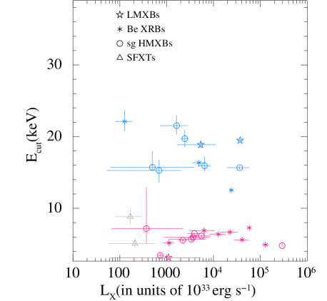
Figure 1: Plot of cutoff energy versus the X-ray luminosity. To identify the apparent dichotomy, we mark the two groups in blue and magenta with SFXTs marked in grey.

When the measured values of the $E_{\rm{cut}}$ are plotted against $L_{\rm{X}}$, we note a bimodality in the $E_{\rm{cut}}$ distribution (see Fig. 1). For clarity, we have used different colour schemes to distinguish the two groups. The upper branch where the cutoff energy range from $\sim$ 12-25 keV (henceforth Branch 1) has been plotted in blue while the lower branch which have cutoff energy range of 3-10 keV (henceforth Branch 2) has been plotted in magenta. Although there is not a clear correlation or anti-correlation among the sources in the two groups, they appear clearly distinguished on the $E_{\rm{cut}}$-$L_{\rm{X}}$ plane. The sources in Branch 1 are: Her X-1, 4U 0115+63, Cen X-3, 4U 1626-67, 4U 1907+09, 4U 1538-522, GX 301-2, Cep X-4, IGR J16393-4643, IGR J16318-4848, and V0332+54. The sources in Branch 2 are: Vela X-1, XTE J1946+274, 1A 1118-61, 4U 0114+65, GX 304-1, OAO 1657-415, 4U 1700-37, GRO J1008-57, 4U 1909+07, 4U 2206+54, SW J2000.6+3210, SMC X-1, EXO 2030+375, 4U 1822-37, KS 1947+300, IGR J16207-5129, IGR J17544-2619, and IGR J18410-0535. Given that the nature of companion stars among the two lists is mixed (see Table. 1 of Sidoli & Paizis, 2019), we see that this bi-modal behaviour cannot be distinguished on the basis of their companion (Be XRBs or supergiants) as illustrated in the Corbet diagram for the X-ray pulsars in our study in Fig.2.

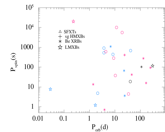
Figure 2: Corbet diagram of the pulsars in our study. Sources marked in blue and magenta are for the sources with cutoff energy greater than and less than 10 keV respectively. As seen in the plot, the distinction is not on the basis of the companion star being a Be X-ray binary or and OB star.

Since we find only three sources with $E_{\rm{cut}}$ within the range of 7-14 keV, there appears to be a paucity of sources with $E_{\rm{cut}}$ around 10 keV, which is the same energy range where there is a gap between the XIS and PIN energy band. We therefore checked if this distribution is an artifact of the energy ranges considered here by simulating several fake spectra with varying cutoff energies distribute from 4-20 keV and fitting them. For all these fake spectra, we recovered the same spectral parameters as the input model thereby validating the robustness of our results.

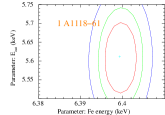
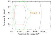
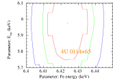
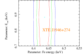
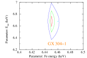
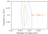
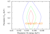
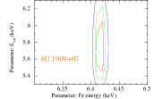
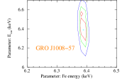
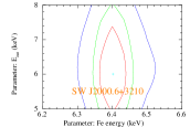
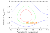
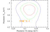
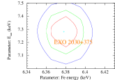
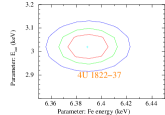
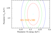
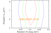
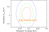
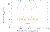
Figure 13: Contour plots between cutoff energy and iron line energy for sources in group 2 where these two values are close to each other. Note that for most of the sources, the iron line energy is centered at the neutral K$\alpha$ line energy of 6.4 keV.

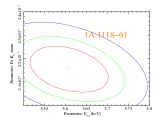
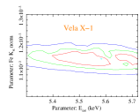
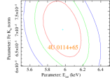
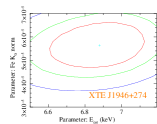
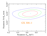
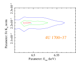
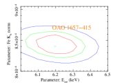
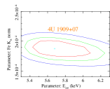
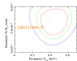
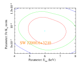
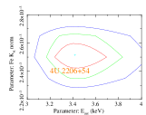
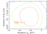
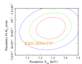
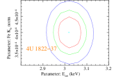
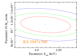
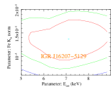
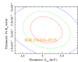
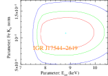
Figure 14: Contour plots between cutoff energy and iron line normalization for sources in group 2 (magenta) where these two values are close to each other

Additionally, since the cutoff energies in the second group are spread around 6 keV, and most of the sources exhibit an iron emission line around 6.4 keV, there may be concerns about a possible mix-up between the iron line and cutoff energies for these sources. However, it should be noted that since the iron line emission in these sources are narrow features and prominently stand out in the X-ray emission, we can easily disentangle between iron line and continuum parameters for a CCD spectrum. We also cross-checked this by simulating several fake spectra with varying cutoff energies (3-7 keV) and narrow iron lines of different equivalent width and were able to fully recover the input parameters, hence supporting our claim. Furthermore, there is no correlation between the cutoff energy and the iron line parameters as seen in the confidence plots for the iron line energy versus the cutoff energy, and the iron line normalization versus the cutoff energy for this group in Fig. 13 and Fig 14 in the Appendix.

In order to test the bi-modality against reported values in literature, we also checked the cutoff energy in literature (with RXTE) obtained using the same model as in this work. These values are tabulated in Table 5. We make a histogram of these literature values and the ones we obtain from our work and find that although for some sources, the cut off energy is different in these two instruments, an apparent bi-modality is visible in both the cut-off energy distribution as seen in top panel of Fig. 3. It should be pointed out that we do not expect a one-to-one correspondence on the values of cutoff energies from these two instruments since they cover different energy ranges and also because for some sources, the X-ray spectrum evolve with flux (see Reig & Nespoli 2013). The interesting finding here is the apparent bi-modal distribution of cut-off energy for sources even within the same class.

We also carried out a number of statistical tests to quantify the bi-modality in the distribution of cut-off energy so obtained. We first performed a 2D KS test for these two branches. The 2D test allow us to compare how different the two distributions are from each other. For the $L_{\rm{X}}$  versus $E_{\rm{cut}}$ variation for red and green groups, the $p$ value is low ($\sim$ 1$\times$10^-5) indicating that these two distributions are different.

However, since our main finding is the bi-modality in the distribution of cut-off energy, we next focus on this. We performed a Dip test (Hartigan & Hartigan, 1985) and obtained a $p$-value of 0.15. The rule of thumb for interpretation of this test is that $p$-values less than 0.05 indicate significant bimodality and values in the range of 0.05-0.10 suggest bimodality with marginal significance. Therefore, while the Dip test do not favor multimodality in the cut-off energy, it should be remarked that this Hartigan’s Dip test work best for small samples but with large bumps. The alternative approach is therefore to search for modes in the data distribution by generating the probability densities of the cut-off energies. In order to do this, we first calculate the best value of band-width based on Silverman’s band-width test and then look for points of inflexion in the Kernel (probability) Density Estimates (KDE) using this band-width as the smoothing function. As seen in the middle of Fig. 3, we find two points of inflexion at $\sim$ 5.7 and 17.8 keV. In the same plot, we have also over-plotted the probability density of histogram using the bin size as the band-width to demonstrate bi-modality.

Finally, we also fit the frequency estimate obtained from histogram with a single Gaussian and two Gaussian functions. As seen from the lower panel of Fig. 3, the histogram is better described by a two Gaussian function ($\chi^{2}_{\rm red}$ $\sim$ 0.7) and a single Gaussian simply fail to fit and result in large ($>$30) values of $\chi^{2}_{\rm red}$.

Next, we extracted the PIN pulse profiles (15.0-70.0 keV) for the pulsating sources in each branch to check if a different beaming mechanism (fan or pencil; Davidson & Ostriker 1973; Burnard, Arons & Klein 1991) could be at the origin of the observed bi-modality. As shown in Fig. 4, the single and double peaked pulse profiles indicating pencil and fan beam respectively are spread out in both groups at random. We therefore also conclude that the current bi-modality in the distribution between $E_{\rm{cut}}$ and $L_{\rm{X}}$ is not based on the beaming pattern of X-rays. As the beaming pattern depends on the accretion rate, $\dot{M}$, the bi-modality is independent of beaming pattern and the accretion rate as well. That the bi-modality in $E_{\rm{cut}}$  is independent of the X-ray luminosity (and hence the accretion rate), can also be see from Fig. 1. We maintained the same colour scheme for the different sources in all other figures that we describe in the following sections to investigate alternative possibilities that could give rise to the observed behavior.

We inspected the ratio of the source spectra to Crab to see if the $E_{\rm{cut}}$  values measured are also evident in the Crab spectral ratio. We however found that since CRSF is rather strong for many sources, the spectral curvature is affected by this absorption feature in the X-ray spectrum for many sources and bi-modality therefore is not straightforward to interpret from this exercise.

Furthermore, in order to check the robustness of our results, with another model, we also tried fitting the 29 sources (that required a cutoff energy) with another phenomological model ‘FDCUT’ in XSPEC . We could reasonably fit 26 sources with FDCUT, albeit with much higher reduced chi-square than HIGHECUT for each source. We find that even when fitting with FDCUT, there are two branches distinguished in the $L_{\rm{X}}$ versus $E_{\rm{cut}}$ plane – similar to what we see with HIGHECUT. Note, however that since the cutoff energies for both these models are mathematically different from each other, their numerical values do not match.

All these factors indicate that the bi-modality in the X-ray spectral shape of these groups are possibly real and further investigations with physical models will allow us to further understand the cause for this. Such detailed studies is however beyond the scope of this current work.

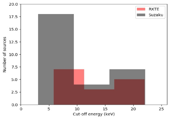
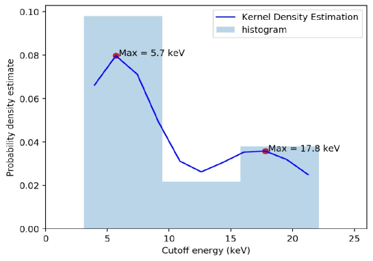
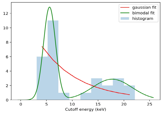
Figure 3: Top: Histogram of cutoff energies from RXTE in red and the current work in gray. The RXTE measurements are indicative of the bi-modality as found in the Suzaku measurements. Middle: The KDE plotted (with a chosen Silverman bandwidth of 3) demonstrate that there are two peaks in the data at $\sim$ 5.7 keV and $\sim$ 17.8 keV respectively. Bottom: The shaded blue region is the histogram for Suzaku data with finer binning compared to top and middle figure. The histogram fits well with a bi-modal function plotted in green as compared to single Gaussian fits shown by red line (the trailing edge of Gaussian).

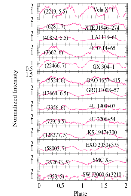
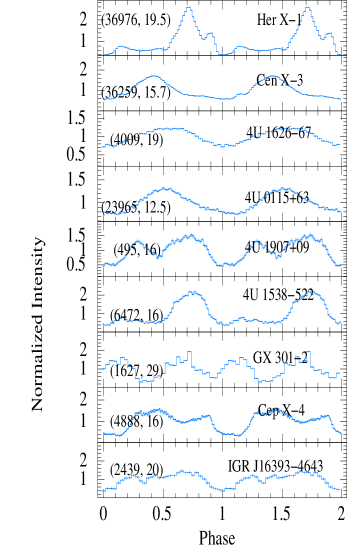
Figure 4: Left: HXD-PIN (15-70 keV) pulse profiles of pulsars in the magenta branch. Right (top): HXD-PIN (15-70 keV) pulse profiles of pulsars in the blue branch. The first number in parenthesis in both the figures is the X-ray luminosity in units of 10³³ erg/s and the second number is the cutoff energy in keV. Right (bottom): Pulse profiles for three sources, LMC X-4, GX 1+4 and A 0535+026 which could not be fit with the HIGHECUT model. See text for details.

4.1.2 $\Gamma$ versus $L_{\rm{X}}$

We report the dependence of $\Gamma$ as a function of $L_{\rm{X}}$ in the case of neutron star HMXBs (including Be XRBs, SGXBs, SFXTs and a few LMXBs), accreting high magnetic field NS in LMXBs spanning over five orders of magnitude in X-ray luminosity. As we show in top of Fig. 5, we find that for all these sources $\Gamma$ and $L_{\rm{X}}$ are marginally anticorrelated with the best-fit to all our data as: $\Gamma$ = a log L_X33 + b, where a = -0.25 $\pm$ 0.04, b = 1.93 $\pm$ 0.15. The dependence of $\Gamma$ as a function of $L_{\rm{X}}$ in the case of Be XRBs have been previously investigated by Reig & Nespoli (2013) who found that $\Gamma$ and $L_{\rm{X}}$ anticorrelate with the X-ray flux during the low X-ray intensity (sub-critical) states of these sources, while a positive correlation is measured during the high intensity (super-critical) states. Their study spanned two orders of magnitude variation in $L_{\rm{X}}$.

It should be noted that most of the sources in our sample are in the sub-critical luminosity regime (see section 5) and our findings are therefore consistent with the anti-correlation seen by Reig & Nespoli (2013) for individual sources.

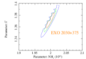
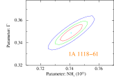
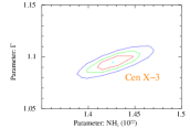
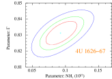
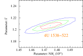
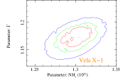
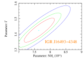
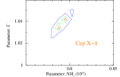
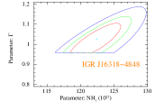
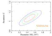
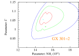
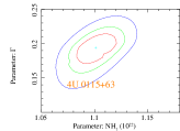
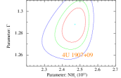
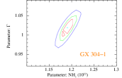
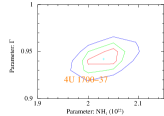
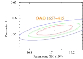
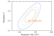
Figure 15: Contour plots between NH1 and gamma

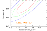
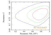
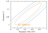
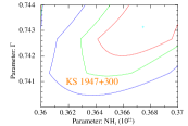
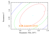
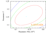
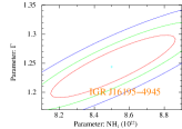
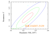
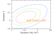
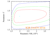
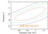
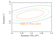
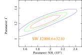
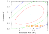
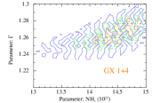
Figure 16: Contour plots between NH1 and gamma

The luminosity span in the current work is however much larger than the RXTE observation of Reig & Nespoli (2013) and while the RXTE observations focused on the evolution of spectra for individual sources (using multiple observations of same Be XRB pulsars at different luminosities), we focus on the overall ‘class’ behaviour of the sources as a function of luminosity. Another improvement with the previous paper is that for the RXTE observations, the authors froze the N_H values for most of the sources while in our analysis - given the better low energy coverage of XIS - we were able to constrain both the photon index and the N_H independently (see contour plots, Fig. 15 and Fig. 16 in Appendix) in most cases.

4.1.3 $E_{\rm{fold}}$ versus $L_{\rm{X}}$

In models of the X-ray spectrum, $E_{\rm{fold}}$ is a measure of the electron temperature of the infalling plasma. An anti-correlation between luminosity and $E_{\rm{fold}}$  has been reported earlier for individual sources like A 0535+26, RX J0440.9+4431, for example (Müller et al., 2013; Ferrigno et al., 2013). It is for the first time that we present here a comprehensive behaviour of the $E_{\rm{fold}}$ dependence on $L_{\rm{X}}$ using a wider sample. In the bottom panel of Fig. 5, we see that with increasing luminosity, the $E_{\rm{fold}}$ value show a weak anti-correlation with the Pearson co-efficient for these two quantities being -0.19.

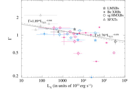
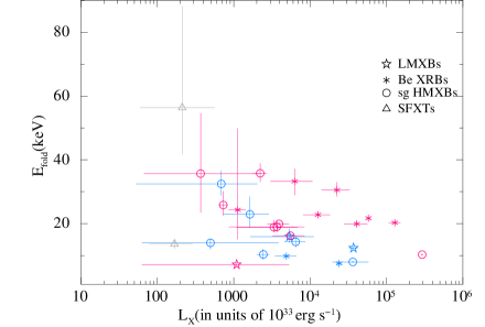
Figure 5: Top: Variation of photon index with luminosity. The black solid line represents the best-fit to the data ($\Gamma\propto L_{\rm{X}}^{-{\alpha}}$ with $\alpha$ = 0.058 $\pm$ 0.006 when sources fit with only XIS spectrum fits are excluded (see section 3, third-last paragraph). The best fit to all the data points (marked in dotted line) is $\alpha$ = 0.068 $\pm$ 0.006 ). The sources A 0535+26, GX 1+4 and LMC X-4 have been marked in black. Bottom: The variation of $E_{\rm{fold}}$ energy with X-ray luminosity. Both the figures are marked with the same colour coding as in Figure 1.

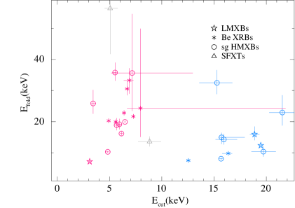
Figure 6: Variation of $E_{\rm{fold}}$ with $E_{\rm{cut}}$ marked with the same colour coding as in Figure 1.

4.1.4 $E_{\rm{fold}}$ versus $E_{\rm{cut}}$

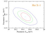
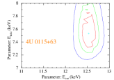
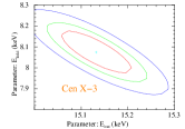
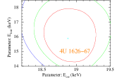
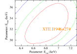
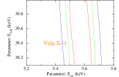
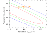
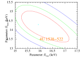
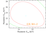
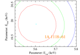
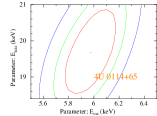
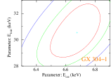
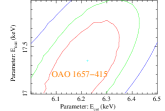
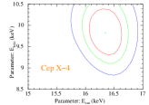
Figure 17: Contour plots between cutoff energy and folding energy

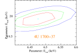
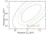
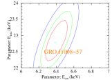
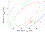
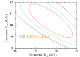
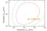
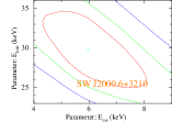
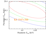
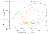
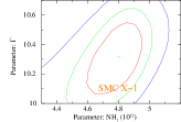
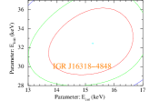
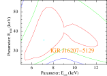
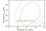
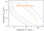
Figure 18: Contour plots between cutoff energy and folding energy

We find that the sources in Branch 2 (magenta) have a somewhat larger median of $E_{\rm{fold}}$ than those in Branch 1 (blue). A plot of their variation is shown in Fig. 6. We remark here that we could independently constrain both the $E_{\rm{cut}}$ and $E_{\rm{fold}}$ as seen in the confidence plots in Appendix (Fig. 17 and Fig. 18) and there is no degeneracy between these two quantities for both groups.

A similar correlation between these two quantities has also been reported earlier by Makishima et al. 1999 where the cutoff energies seem to be divided into two groups (their Fig. 12 b) less than and above 10 keV. The authors however do not comment about this in their paper.

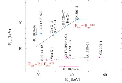
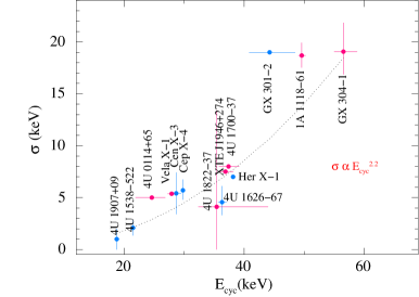
Figure 7: Left: $E_{\rm{cut}}$ versus E_cyc showing two scaling laws for two groups. Right: Positive correlation between CRSF width $W_{\rm c}$ versus E_cyc. All the figures are marked with the same colour coding as in Figure 1.

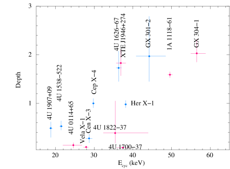
Figure 8: Plot of CRSF depth versus CRSF energy. All the figures are marked with the same colour coding as in Figure 1.

4.1.5 $E_{\rm{cut}}$ versus E_cyc

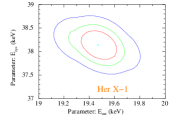
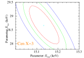
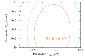
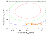
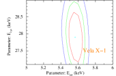
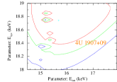
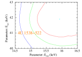
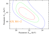
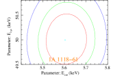
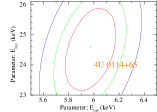
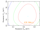
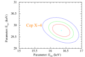
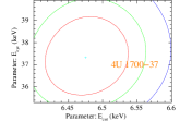
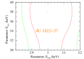
Figure 19: Contour plots between cutoff energy and cyclotron line energy

The variation of $E_{\rm{cut}}$ with E_cyc for HMXBs has been investigated in earlier works. Coburn et al. (2002) and Makishima et al. (1999) used RXTE and Ginga data respectively to obtain the relationship E_cut $\propto$ E${}_{cyc}^{0.7}$ for E_cyc below 35 keV. Thanks to the broadband spectral capability of Suzaku, in our analysis, we show that the correlation between these two quantities (contour plots in Fig. 19 in Appendix) is not unique but rather have a complex behaviour (left of Fig. 7). The sources in blue branch can be fitted to a functional form of $E_{\rm{cut}}$ $\propto$ E${}_{cyc}^{0.82\pm 0.08}$ (marked by the black line). The functional form for sources in magenta is $E_{\rm{cut}}$ $\propto$ E${}_{cyc}^{0.29\pm 0.06}$ (black dashed line). In order to make a comparison with the latest result, we digitized the graph in Staubert 2003 to fit their Fig. 8 and find that in their work, they report: $E_{\rm{cut}}$ $\propto$ E${}_{cyc}^{0.47(-0.35,0.39)}$ which is consistent with our results for both groups within errors.

It should however be noted that if we allow for an offset, we get a different best fit result of $E_{\rm{cut}}$= 8 $+$ E${}_{cyc}^{0.67}$ and $E_{\rm{cut}}$= 5 $\times$ E${}_{cyc}^{0.36}$. Therefore, while various forms work in the correlation between these quantities and the correlation is not mathematically unique, it is evident visually that the blue branch does have a steeper slope in this graph. We also remark here that the values of E_cyc we obtain from this work are close to values obtained in Coburn et al. 2002. The difference between the Figure 9 of Coburn et al. 2002 and Figure 7 of this work is a result of the determination of the values of $E_{\rm{cut}}$ which is possibly not surprising since we do not expect a one-to-one correspondence on the values of cutoff energies from RXTE and Suzaku as they cover different energy ranges and also because for some sources, the X-ray spectrum evolve with flux (see Reig & Nespoli 2013).

4.1.6 CRSF width $W_{\rm c}$ versus E_cyc

The variation of the CRSF width versus E_cyc is shown on the right side of Fig. 7. In agreement with the results of Coburn et al. (2002), we observe a linear correlation between the two quantities. We are aware that using a HIGHECUT model can sometimes lead to artificial widening of the CRSF energy if E_cyc and $E_{\rm{cut}}$ are close to each other. To mitigate this, we took great care in constraining the width of the CRSF properly and cross-checked the values with those available in literature. For example, the three sources (1A 1118-61, GX 301-2 and GX 304-1), where we obtain large widths are consistent with their literature values (Suchy et al., 2012, 2011; Jaisawal, Naik & Epili, 2016). From our fits of the broadband data, we find $W_{c}$ $\propto$ E${}_{cyc}^{~{}(2.2\pm 0.5)}$. Overall, as we see from Table LABEL:continuum and in Fig. 8 that the higher the value of cyclotron line energy, the deeper the line is.

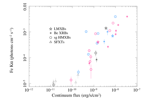
Figure 9: Plot of the iron line flux versus continuum flux marked with the same colour coding as in Figure 1.

4.1.7 Fe K$\alpha$ flux versus continuum flux

From Fig. 9, we see that the Suzaku data of the considered sources suggest a strong correlation between the continuum flux and the Fe K$\alpha$ flux. Such a correlation is expected and was also previously reported by Giménez-García et al. (2015) and Torrejón et al. (2010) but over a smaller range of continuum flux.

4.1.8 Equivalent Width (EW) of K$\alpha$ iron line versus $L_{\rm{X}}$

On the right side of Fig. 9, we show the lack of any clear correlation between the equivalent width of the iron K$\alpha$ line and the source X-ray luminosity. An anticorrelation between these two parameters have been reported earlier in the literature by Giménez-García et al. (2015), Vasylenko, Zhdanov & Fedorova (2015), and Torrejón et al. (2010). This anticorrelation is usually interpreted in terms of the so called Baldwin effect (Baldwin, 1977). As previous studies were carried out in a limited energy range, we checked that our results did not change when only the XIS data are used to fit the spectra (with a powerlaw corrected for photoelectric line-of-sight absorption and Gaussian) of all the sources (0.8-10 keV). We also performed the same study by using the restricted energy range 7.1-12.0 keV to estimate the X-ray luminosity of each source (only photons above 7.1 keV contribute to the K$\alpha$ emission and the photoelectric cross section drops rapidly so that photons above 12 keV do not contribute much in this process) and the energy range 4.95-7.75 keV as done in Torrejón et al. (2010). In none of these cases we could find a clear indication of the anticorrelation reported previously. In addition, we have also explored similar correlation using XMM data in a different work where we do not find any such relation between EW and luminosity (see Fig. 2 of Pradhan, Bozzo & Paul 2018).

The existence of this X-ray Baldwin effect has been a matter of much debate for AGNs and possibly depend on different class of AGNs. A systematic analysis of many AGNs using XMM and INTEGRAL data showed a very weak correlation between the EW of Fe K$\alpha$ line and luminosity (see Vasylenko, Zhdanov & Fedorova 2015 and references therein). We will return to this discussion in section 5.

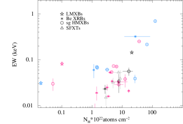
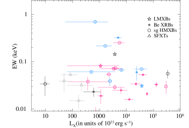
Figure 10: Left: Plot of the equivalent width versus luminosity. Right: Plot of absorption column density versus the EW of iron line. We use for all plots the same color coding of Fig. 1.

4.1.9 Equivalent Width (EW) of K$\alpha$ versus ${N_{\rm H}}$

As visible from Fig. 10, we found a clear linear correlation between the hydrogen column density of the different sources and the equivalent width of their K$\alpha$ lines. Here ${N_{\rm H}}$ = ${N_{\rm H1}}$+${N_{\rm H2}}$*${C_{V}}$, where ${N_{\rm H1}}$ is the hydrogen column density along our line of sight to the source, ${N_{\rm H2}}$ accounts for local absorption and ${C_{V}}$ is the covering fraction, the latter having a wide range of 0.1-0.96 (see Table LABEL:continuum).

Generally, it is well known that when a relatively limited energy range is used for the X-ray spectral fitting on data with limited statistical quality (eg 0.5-10.0 keV), the derived values of the absorption column density and the power-law spectral index can be positively correlated (a larger absorption column density can be used in such restricted energy range to fit the spectrum equally well with a steeper power-law). We also checked apriori the variation of $\Gamma$ as a function of ${N_{\rm H}}$ to cross-check some of our results and find that this is not the case for our spectral analysis, mainly thanks to the wide energy coverage of the instruments onboard Suzaku (see contour plots, Fig. 15 and 16 in the Appendix).

5 Discussion

In this paper, we took advantage of the broad energy coverage of the instruments on-board Suzaku to perform a systematic study of all observed neutron star HMXBs, including the high magnetic field LMXB pulsars displaying a cyclotron absorption line in their spectra. The aim of our analysis was to explore a number of correlations between the spectral parameters of these sources reported previously in the literature. We used for the analysis of all sources a similar spectral model, in order to carry out a consistent investigation of all their spectral parameters. While detailed individual studies of most of these sources are already reported in literature, our aim with this paper is to outline a comprehensive behaviour of HMXBs as a class. Such a study was last carried out nearly two decades back in early 2000s (Coburn et al., 2002).

We summarize the main results of the paper below:

1. The broadband X-ray spectra of all HMXBs that we considered in this paper can be described by a powerlaw component modified by a cutoff energy (where PIN data is usable). This spectral shape is usually interpreted in terms of Comptonization of the seed photons produced in the thermal mound of the neutron star accretion column by free electrons in the accreting material. It is therefore expected that the spectral cutoff energies are proportional to the electron temperature.
   A lack of correlation between $E_{\rm{cut}}$ and $L_{\rm{X}}$ has been reported earlier by White, Swank & Holt (1983). They point out, however, that the low luminosity systems in their sample do exhibit a somewhat less sharp cutoffs at higher energies.
   In this study, we found all analyzed systems distributing on two different branches in the $E_{\rm{cut}}$ and $L_{\rm{X}}$ plot. For sources in Branch 1 (represented in blue in all plots), the cut-off energy, that is a measure of the electron temperature, vary from 12-24 keV and increases with the mass accretion rate (in turns regulating the X-ray luminosity). For sources following the Branch 2 (magenta), $E_{\rm{cut}}$ remains in a narrower range from 3-10 keV, even when $L_{\rm{X}}$ changes by a factor of $\sim$ 1000. This result indicates that the cutoff energies of the sources do not depend only on the luminosity. As we showed in Section 3, this different behaviour cannot either be simply ascribed to switches between a pencil and a fan beam emission geometry due to the lack of clear systematic variations in the pulse profiles of the analysed sources. To the best of our knowledge, so far, no theoretical explanation has been proposed in the literature to interpret this behaviour.

2. An anticorrelation between $\Gamma$ and $L_{\rm{X}}$ is known to exist in neutron star LMXBs and black hole systems (for luminosities lower than ‘critical’ luminosity) where accretion takes place through a disc (Allen et al., 2015; Wu & Gu, 2008). Wijnands et al. (2015) suggested that in case of strongly magnetized neutron stars the presence of a magnetic field could significantly alter the spectra, such that a direct comparison between HMXBs and LMXBs is not possible. For the present study, we make use of systems containing in all cases strongly magnetized neutron stars (B $\gtrsim$ $10^{12}$ G) and accreting both from disks and from stellar winds. We found that the anticorrelation between $\Gamma$ and $L_{\rm{X}}$ still holds, indicating that in HMXBs, the Comptonization process makes the spectrum harder at increasing $L_{\rm{X}}$ at least in the sub-critical regime (even though it might break down at luminosities higher than $10^{37}$ ergs $s^{-1}$).

   For black hole binaries, since this anti-correlation is valid for luminosities below a critical value, we also cross-checked the X-ray luminosity of each pulsar against the critical luminosity of each pulsar using Eqn. 3 (Becker et al., 2012) below.

   $$L_{\rm crit}=1.49\times 10^{37}{\rm erg\,s}^{-1}\times\left(\frac{\Lambda}{0.1}\right)^{-7/5}\times w^{-28/15}\times\left(\frac{M}{1.4{\rm\,M}_{\odot}}\right)^{29/30}\left(\frac{R}{10{\rm\,km}}\right)^{1/10}\left(\frac{B_{\rm surf}}{10^{12}{\rm\,G}}\right)^{16/15}$$ (3)

   where $R$, $M$, and $B$ are, the radius, mass, and surface magnetic field strength (B in terms of $\sim 10^{12}$ G) of the neutron star, $\Lambda$ $=$ 1, and $w=1$ for wind-accreting systems. For all those sources with measured B (through CRSF line energy), we find that besides Her X-1, 4U 0115+63, Cen X-3 and 1A 1118-61, all other sources are indeed in the sub-critical regime.

3. An anticorrelation of $E_{\rm{fold}}$ with $L_{\rm{X}}$ indicates that with increasing luminosity, $E_{\rm{fold}}$ (a proxy for electron temperature of the ‘infalling’ plasma) decreases. As the luminosity increases, the radiation field from the neutron star begin to affect the accretion flow and Compton cooling becomes more efficient (since scattering rate of photons off electrons increase). This leads to the shift of electron temperature toward lower energies with increasing luminosity giving rise to this anticorrelation of $E_{\rm{fold}}$ with $L_{\rm{X}}$.

4. From the variation of folding energy with cutoff energies, we see that smaller cutoff energy imply larger folding energies. It has also been reported by earlier authors that the non cyclotron-line pulsars should exhibit larger values of folding energy, (less steep spectral breaks) due to their lack of the spectral trough caused by an absorption like feature in CRSF (Makishima et al., 1999). However, when we compared the folding energy of cyclotron line sources with the folding energy of non-cyclotron line sources, we see no such trend.

5. The variation of $E_{\rm{cut}}$ with E_cyc has been studied in a number of earlier works (Makishima et al., 1990, 1999; Coburn et al., 2002). Makishima et al. (1990) obtained a linear correlation between $E_{\rm{cut}}$ and E_cyc (E_cyc = 1.4-1.8 $E_{\rm{cut}}$). From the measurements of $E_{\rm{cut}}$, they thus inferred that the magnetic field of HMXBs was spanning a relatively narrow range (1-4 $\times 10^{12}$ G). Nine years later, these results were updated by Makishima et al. (1999). These authors used a larger sample of sources to prove that there exists a saturation of $E_{\rm{cut}}$ at high values of E_cyc ( $E_{\rm{cut}}$ $\propto$ E${}_{cyc}^{0.7}$). They interpreted this finding by suggesting that the presence of a thermal emission component can affect the position of the spectral energy break. Coburn et al. (2002) reconfirmed the same relationship, adding also new constrains on the saturation of $E_{\rm{cut}}$ . The latter seems to be detected only below 35 keV. They also suggested the possible presence of two linear relations between $E_{\rm{cut}}$ and E_cyc, one below 35 keV and one above. Our current study has an added advantage of the broadband energy coverage compared to these previous works in literature. We find that for higher values of magnetic field, the cutoff energies tend to saturate for both these groups. This is possibly because there could be some other relativistic effects in the creation of the continuum that become important at at higher values of magnetic field.

6. The right panel of Fig. 7 shows that in the present study we found a relatively well marked linear correlation between the energy of the cyclotron line and it’s width. Coburn et al. (2002) mentioned that the FWHM of a CRSF changes with the viewing angle $\theta$ of the observer with respect to the magnetic field as follows:

   $$W_{\rm c}\propto E_{\rm{C}}\sqrt{kT_{\rm e}}\left|\cos(\theta)\right|$$ (4)

   This implies that two quantities, the characteristic electron temperature, $kT_{\rm e}$  and $\theta$ (angle between the observer line of sight and the neutron star magnetic field) for all sources considered in this paper are not dramatically different. The same linear correlation was also found by Coburn et al. (2002) and are indicative of small values of $kT_{\rm e}$ . The reason for this is that the matter being accreted onto the hot spots form an accretion column and in the steady state, the amount of matter falling in balances the matter spreading out at the base where the mound parameters (area, density etc) are similar for most sources irrespective of accretion rate. Our results support their argument since despite five orders of magnitude change in $L_{\rm{X}}$ in the current work, our findings are indicative of the same linear correlation. Alternatively, this correlation can also be explained if the temperature is tied to the magnetic field strength as seen in some simulations of gamma-ray bursts (Lamb, Wang & Wasserman, 1990).

   Another implication of this relation is that, any effect of $\theta$ is also very small. Since the bulk motion of the electrons (which in turn depend on the accretion rate) also play a role in line broadening, we should have expected this correlation to smear out. This brings us to a very interesting point as has been discussed in Coburn et al. (2002) that accretion could have an influence on the relative orientation of spin and magnetic axes, with the spin axis presumably being influenced by the age of the system and the accretion timescales making $\theta$ very small. This correlation can be further tested for individual sources by detailed pulse profile modelling of each source and measuring the width of the CRSF line with varying $\theta$.

   It is interesting to mention here that in Staubert et al. 2019, there are two groups in width of CRSF versus energy (their Fig. 12) where the authors argue that the second slope are mostly consist of ‘outlier” sources. We find similar scatter in the depth of CRSF versus CRSF energy (Fig. 8) although the sources do not hold a on-to-one correspondence in both the works.

7. Our analysis also confirmed the presence of a strong correlation between the X-ray continuum of all the sources where a K$\alpha$ iron emission line is found and the line flux. This is expected, since the Fe K$\alpha$ line is thought to be produced in these systems due to the reprocessing of the X-ray continuum by iron atoms in the matter surrounding the neutron star (being either the material from the stellar winds in HMXBs or the disk in LMXBs). As was also discussed by Torrejón et al. (2010) and Giménez-García et al. (2015), we thus expect the Fe K$\alpha$ line flux to increase with the flux of the continuum.
   

   Historically, an inverse correlation was obtained between the EW of C IV lines and the UV luminosity in AGNs (Baldwin effect; Baldwin 1977). Analogously, correlation studies between the EW of K$\alpha$ lines and $L_{\rm{X}}$ have been carried out for AGNs and XRBs providing indications for an inverse correlation (Giménez-García et al., 2015; Vasylenko, Zhdanov & Fedorova, 2015; Torrejón et al., 2010). This anticorrelation between the EW of K$\alpha$ lines and $L_{\rm{X}}$ is called the X-ray Baldwin Effect. At odds with the results of Giménez-García et al. (2015) and Torrejón et al. (2010), we did not detect any significant correlation between the EW of the Fe K$\alpha$ lines and the source X-ray luminosity. As discussed by Torrejón et al. (2010), we noticed in our case that a marginal correlation (not statistically significant) is visible when the EW of the K$\alpha$ line is plotted against the X-ray flux but the correlation disappears when the luminosity is used in place of the flux.

   The non-confirmation of the X-ray Baldwin effect for the Fe K_α in X-ray binaries is probably not surprising since there is no physical reason for the effect to hold true for XRBs with the neutral iron line. In case of AGNs the physical reason for the anti-correlation of EW of C_IV lines with luminosity is that for higher luminosity the atoms are highly ionised and do not produce C_IV lines in same proportion. However, in the case of the neutral 6.4 keV iron line in X-rays, if the increase in luminosity cause the ionisation to be so high as to remove the K-shell electrons, we should be seeing the Hydrogen like and Helium like iron atoms and the iron line would instead be seen at 6.7 and 6.9 keV instead of the neutral K_α line at 6.4 keV. On the contrary, very few HMXBs like Cen X-3 (Naik, Paul & Ali, 2011), OAO 1657-415 (Pradhan, Raman & Paul, 2019),for example, show these emission lines.

8. Finally, we also reported on the positive correlation between the EWs of the iron K$\alpha$ line and the absorption column density local to the HMXB sources (${N_{\rm H}}$). This correlation is expected because a larger ${N_{\rm H}}$ implies that more stellar wind material around the neutron star is involved in the formation of a stronger iron line (see e.g., Inoue 1985; Pradhan et al. 2014, 2015; Giménez-García et al. 2015; Pradhan et al. 2019) except in some sources with accretion disk like SMC X-1, where a relatively low column density is seen (Pradhan, Maitra & Paul, 2020). In others like the persistent Be XRB, SW J2000.6+3210, the iron line is almost undetectable since there is not enough matter surrounding the neutron star to facilitate fluorescence (Pradhan et al., 2013).

   Although we have very few SFXTs compared to classical sg HMXBs in the current work, we note that the absorption column density (and EW) for these SFXTs are smaller when compared to classical sgXBs (see Table LABEL:continuum). This motivated us to look into our findings with more details by including a larger sample of SFXTs. We also therefore extended this study by including XMM data and have discussed the findings in detail in Pradhan, Bozzo & Paul 2018 which we refer to the reader for further details. We find that the lower N_H and lower EW should be expected for SFXTs. Such a difference is either due to faster (or rarer) stellar winds in SFXTs or due to the inhibition of accretion in SFXTs most of the time by other mechanisms like magnetic gating (Bozzo, Falanga & Stella, 2008) leading to inefficient photoionization of the stellar wind.

   We reported in the plots of Fig. 9 and Fig. 10 also the LMXBs considered in this paper for completeness, but we do not expect them to follow a similar correlation as for the HMXBs. For LMXBs, the iron line is indeed supposed to have a completely different origin than in HMXBs (see, e.g. Cackett & Miller 2013).

The residuals from all the best fits to the data of the different sources are shown in Fig. 11 and 12 and various contour plots are shown in the Appendix.

6 Summary

In this section, we summarize the main results of our work discussed above. This class analysis of the broad band X-ray spectrum of 39 accreting neutron star X-ray binaries indicate some interesting findings. (i) We find that the relationship between the cut-off energy and X-ray luminosity follow a bi-modal behaviour. The interpretation of such a dichotomy is not straightforward and is not a result of different companion stars (LMXBs, Be XRBs, sgXBs) or beaming patterns (explored through pulse profiles). We encourage further studies using physical continuum and line models in order to investigate this behaviour. (ii) We also find that the dependence of cut-off energies on the CRSF energy is not unique. We also confirm the previous findings of Coburn et al. 2002 that the width (and depth) of the CRSF is linearly correlated to the CRSF energy. (iii) We confirm the correlation between the iron K$\alpha$ emission line and the X-ray continuum flux, between the EW of the iron K$\alpha$ line and absorption. This is expected since such lines are formed by the fluorescence of the X-ray continuum photons in interstellar matter around the NS in case of HMXBs. We also note that the EW and absorption are different between SFXTs and classical HMXBs and interpret that as being caused by difference in stellar wind properties between these two systems or a result of inhibited accretion in SFXTs during most times. Finally, (iv) we note that the photon index and $E_{\rm{fold}}$  is negatively correlated with luminosity, thus suggesting that Compton cooling becomes more efficient at higher luminosities which makes the spectrum harder and also lowers the electron temperature of the plasma.

Overall, we have updated the correlation between spectral parameters of accreting neutron stars taking advantage of the broadband energy coverage of Suzaku. Such a study was long overdue in literature with the last such study made almost two decades back.

Figure 11: Spectra of all considered sources together with residuals from the best fits. All best fit results are reported in Table LABEL:continuum

Figure 12: Spectra of all considered sources together with residuals from the best fits. All best fit results are reported in Table LABEL:continuum..contd

Table 1: Observation Log and distances to the different sources considered in the present paper.

Source	OBSID	WINDOW MODE	DISTANCE (kpc)	Reference
Her X-1	100035010	1/8	6.6 $\pm$ 0.4	Reynolds et al. 1997
4U 0115+63	406049010	1/4	7.0 $\pm$ 0.3	Riquelme, Torrejón & Negueruela 2012
Cen X-3	403046010	1/4	5.7 $\pm$ 1.5	Thompson & Rothschild 2009
4U 1626-67	400015010	1/8	5-13	Chakrabarty 1998
XTEJ1946+274	405041010	1/4	9.5 $\pm$ 2.9	Wilson et al. 2003
Vela X-1	403045010	1/4	1.9 $\pm$ 0.2	Sadakane et al. 1985
4U 1907+09	401057010	1/4	$2.8_{-1.8}^{+5.0}$	Nespoli, Fabregat & Mennickent 2008
4U 1538-522	407068010	1/4	6.4 $\pm$ 1	Reynolds, Bell & Hilditch 1992
GX 301-2	403044010	1/4	3.04∗	Kaper, van der Meer & Najarro 2006
1 A1118-61	403049010	1/4	5.2 $\pm$ 0.9	Riquelme, Torrejón & Negueruela 2012
4U 0114+65	406017010	1/4	7.0 $\pm$ 3.6	Reig et al. 1996
GX 304-1	905002010	1/4	2.4 $\pm$ 0.5	Parkes, Murdin & Mason 1980
OAO 1657-415	406011010	1/4	6.4 $\pm$ 1.5	Chakrabarty et al. 2002
Cep X-4	409037010	1/4	3.8 $\pm$ 0.6	Bonnet-Bidaud & Mouchet 1998
4U 1700-37	401058010	1/4	2.12 $\pm$ 0.34	Megier et al. 2009
A 0535+026	404054010	1/4	2.00 $\pm$ 0.7	Steele et al. 1998
4U 1822-37	401051010	1/4	$2.5_{-1.9}^{+3.0}$	Mason & Cordova 1982
GX 1+4	405077010	1/4	3-15	Chakrabarty & Roche 1997
GRO J1008-57	902003010	1/4	5∗	Coe et al. 1994
4U1909+07	405073010	1/4	7.00 $\pm$ 3.0	Morel & Grosdidier 2005
IGR J16393-4643	404056010	Off	10.6∗	Chaty et al. 2008
4U 2206+54	402069010	1/4	2.90 $\pm$ 0.20	Riquelme, Torrejón & Negueruela 2012
SW J2000.6+3210	401053020	Off	8∗	Masetti et al. 2008
LMC X-4	702036020	1/8	50∗	Hung et al. 2010
KS1947+300	908001020	1/4	10.4 $\pm$ 0.9	Riquelme, Torrejón & Negueruela 2012
EXO 2030+375	402068010	1/4	7.1 $\pm$ 0.2	Wilson et al. 2002
SMC X-1	706030100	Off	60.0∗	Neilsen, Hickox & Vrtilek 2004
V 0332+53	904004010	1/4	7.5 $\pm$ 1.50	Negueruela et al. 1999
IGR J16493-4348	401054010	Off	2-3	Hill et al. 2008
IGRJ16318-4848	401094010	Off	3.60 $\pm$ 2.60	Filliatre & Chaty 2004
IGRJ16207-5129	402065020	1/4	$6.10_{-3.50}^{+8.90}$	Nespoli, Fabregat & Mennickent 2008
IGR J18410-0535	505090010	Off	$3.2_{-1.5}^{+2.0}$	Nespoli, Fabregat & Mennickent 2008
IGR J17544-2619	402061010	1/4	3.20 $\pm$ 1.00	Pellizza, Chaty & Negueruela 2006
IGR J16195-4945	401056010	Off	5∗	Tomsick et al. 2006
IGR J16465-4507	401052010	Off	$9.5_{-5.7}^{+14.1}$	Heras & Walter 2004
IGR J16479-4514	406078010	Off	7.50 $\pm$ 2.50	Chaty et al. 2008
IGR J17391-3021	402066010	1/4	2.7∗	Rahoui et al. 2008
IGR J08408-4503	404070010	Off	3.0∗	Masetti et al. 2006
IGR J00370+6122	402064010	1/4	3.3∗	Reig et al. 2005
∗ Distance error is not known so error is assumed as 1 kpc.

Table 2: Parameters of the continuum and absorption features. Errors quoted are for 90 per cent confidence range

Source

${N_{\rm H1}^{{}_{a}}}$

${N_{\rm H2}^{{}_{a}}}$

${C_{V}}$

$\Gamma$

$\Gamma_{norm}^{b}$

Ecut

Efold

EC1

D1

W1

bb (kT)

$bb_{norm}^{c}$

$\chi^{2}_{\rm red}$/dof

(keV)

(keV)

(keV)

(keV)

Her X-1

0.02

-

-

$0.81_{-0.01}^{+0.02}$

$0.084_{-0.002}^{+0.004}$

$19.47_{-0.14}^{+0.16}$

$12.34_{-0.34}^{+0.35}$

$38.14_{-0.34}^{+0.33}$

$0.98_{-0.07}^{+0.08}$

7

$0.55_{-0.03}^{+0.02}$

$0.00077_{-0.00001}^{+0.00001}$

1.55/661

4U 0115+63

$1.13_{-0.02}^{+0.02}$

-

-

$0.19_{-0.02}^{+0.03}$

$0.025_{-0.002}^{+0.001}$

$12.54_{-0.18}^{+0.16}$

$7.53_{-0.25}^{+0.39}$

9.57

0.67

1.0

$0.59_{0.01}^{0.01}$ $0.0012_{-0.0001}^{+0.0001}$

1.44/436

Cen X-3

$1.43_{-0.02}^{+0.03}$

-

-

$1.09_{-0.01}^{+0.01}$

$0.392_{-0.079}^{+0.089}$

$15.14_{-0.15}^{+0.17}$

$8.07_{-0.31}^{+0.37}$

$28.66_{-0.84}^{+0.82}$

$0.28_{-0.09}^{+0.09}$

$5.41_{-2.03}^{+2.42}$

$0.107_{-0.006}^{+0.006}$

$0.049_{-0.011}^{+0.015}$

1.34/658

4U 1626-67

$0.09_{-0.02}^{+0.02}$

-

-

$0.830_{-0.008}^{+0.008}$

$0.0092_{-0.0001}^{+0.0001}$

$18.87_{-0.44}^{+0.47}$

$15.92_{-1.85}^{+2.51}$

$36.31_{-0.64}^{+0.74}$

$1.73_{-0.28}^{+0.35}$

$4.56_{-1.25}^{+1.54}$

$0.28_{-0.01}^{+0.01}$

$0.00014_{-0.00002}^{+0.00002}$

1.29/910

XTE 1946+274

$1.37_{-0.03}^{+0.03}$

$7.00_{-1.01}^{+1.11}$

$0.25_{-0.04}^{+0.03}$

$1.09_{-0.04}^{+0.03}$

$0.018_{-0.001}^{+0.001}$

$6.89_{-0.52}^{+0.40}$

$33.28_{-4.28}^{+3.87}$

$36.88_{-1.18}^{+1.30}$

$1.83_{-0.26}^{+0.27}$

7.5

-

-

1.12/816

Vela X-1

$1.29_{-0.04}^{+0.03}$

$3.02_{-0.21}^{+0.20}$

$0.43_{-0.03}^{+0.02}$

$1.16_{-0.02}^{+0.02}$

$0.19_{-0.01}^{+0.01}$

$5.53_{-0.23}^{+0.15}$

$35.79_{-2.64}^{+3.15}$

$27.90_{-0.66}^{+0.57}$

$0.102_{-0.023}^{+0.025}$

$5.37$

-

-

1.64/664

4U 1907+09

$2.47_{-0.08}^{+0.06}$

$2.81_{-0.78}^{+0.86}$

$0.24_{-0.06}^{+0.08}$

$1.29_{-0.02}^{+0.01}$

$0.0240_{-0.0008}^{+0.0004}$

$15.71_{-0.27}^{+2.22}$

$14.96_{-2.15}^{+1.46}$

$18.74_{-0.39}^{+0.45}$

$0.49_{-0.19}^{+0.13}$

$1.00_{-1.00}^{+0.99}$

-

-

1.07/882

4U 1538-522

$1.47_{-0.01}^{+0.01}$

-

-

$1.208_{-0.008}^{+0.007}$

$0.0506_{-0.0006}^{+0.0005}$

$15.94_{-0.79}^{+1.26}$

$14.29_{-1.02}^{+0.86}$

$21.46_{-0.45}^{+0.43}$

$0.53_{-0.08}^{+0.11}$

$2.09_{-0.74}^{+0.76}$

-

-

1.22/710

GX 301-2

$14.98_{-0.73}^{+0.72}$

$53.02_{-1.97}^{+1.91}$

0.95

$1.055_{-0.058}^{+0.053}$

$0.068_{-0.009}^{+0.010}$

$21.54_{-1.25}^{+1.45}$

$22.93_{-4.16}^{+5.55}$

$44.20_{-3.40}^{+4.25}$

$1.97_{-0.52}^{+0.82}$

19

-

-

1.11/529

1A 1118-61

$0.74_{-0.01}^{+0.01}$

$0.36_{-0.01}^{+0.01}$

$0.069_{-0.001}^{+0.001}$

$5.58_{-0.09}^{+0.10}$

$19.92_{-0.57}^{+0.61}$

$49.94_{-0.51}^{+0.56}$

$1.59_{-0.06}^{+0.06}$

$18.69_{-1.16}^{+1.22}$

-

-

1.61/468

4U 0114+65

$4.79_{-0.22}^{+0.16}$

$23.15_{-9.85}^{+15.61}$

$0.12_{-0.04}^{+0.05}$

$0.78_{-0.06}^{+0.06}$

$0.011_{-0.001}^{+0.001}$

$5.94_{-0.24}^{+0.22}$

$19.17_{-1.62}^{+1.72}$

$24.53_{-2.71}^{+2.22}$

$0.14_{-0.06}^{+0.05}$

5

$0.138_{-0.006}^{+0.007}$

$0.0180_{-0.0070}^{+0.0093}$

1.17/453

GX 304-1

$1.19_{-0.01}^{+0.02}$

$12.19_{-0.78}^{+0.88}$

$0.28_{-0.02}^{+0.02}$

$1.02_{-0.03}^{+0.02}$

$0.816_{-0.04}^{+0.04}$

$6.68_{-0.20}^{+0.17}$

$30.55_{-2.04}^{+2.37}$

$56.54_{-1.54}^{+2.28}$

$2.03_{-0.18}^{+0.29}$

$19.06_{-2.18}^{+2.78}$

-

-

1.39/673

OAO 1657-415

$16.67_{-0.58}^{+0.54}$

$43.06_{-4.56}^{+5.00}$

$0.45_{-0.03}^{+0.03}$

$0.49_{-0.04}^{+0.04}$

$0.011_{-0.001}^{+0.001}$

$6.14_{-0.16}^{+0.14}$

$16.18_{-0.62}^{+0.67}$

-

-

-

-

-

1.31/420

Cep X-4

$0.79_{-0.02}^{+0.02}$

$90.15_{-30.79}^{+59.39}$

$0.29_{-0.07}^{+0.43}$

$1.04_{-0.03}^{+0.03}$

$0.11_{-0.01}^{+0.08}$

$16.36_{-0.58}^{+0.37}$

$9.82_{-0.58}^{+0.66}$

$29.78_{-0.30}^{+0.30}$

$1.03_{-0.09}^{+0.10}$

$5.70_{-0.90}^{+1.04}$

$1.04_{-0.06}^{+0.08}$

$0.0011_{-0.0003}^{+0.0003}$

1.28/234

4U 1700-37

$2.03_{-0.04}^{+0.04}$

$4.43_{-0.10}^{+0.11}$

$0.70_{-0.01}^{+0.01}$

$0.94_{-0.01}^{+0.01}$

$0.184_{-0.004}^{+0.005}$

$6.48_{-0.07}^{+0.05}$

$19.93_{-0.17}^{+0.39}$

$37.38_{-1.59}^{+1.77}$

$0.09_{-0.02}^{+0.01}$

8

-

-

1.45/654

A0535+026n

$0.74_{-0.04}^{+0.07}$

$5.50_{-0.64}^{+0.86}$

$0.35_{-0.03}^{+0.04}$

$1.14_{-0.05}^{+0.09}$

$0.048_{-0.003}^{+0.005}$

$13.15_{-1.42}^{+4.06}$

-

$41.91_{-0.75}^{+1.02}$

$10.14_{-1.99}^{+3.83}$

$1.43_{-0.20}^{+0.37}$

$0.089_{-0.015}^{+0.013}$

$0.0029_{-0.0012}^{+0.0044}$

1.09/706

4U 1822-37

0.1

-

-

$0.058_{-0.037}^{+0.040}$

$0.0131_{-0.0004}^{+0.0005}$

$3.10_{-0.11}^{+0.14}$

$7.16_{-0.31}^{+0.39}$

$35.41_{-3.06}^{+8.55}$

$0.39_{-0.21}^{+0.66}$

$4.11_{-4.10}^{+9.27}$

$0.189_{-0.008}^{+0.007}$

$0.0003_{-1.06427e-05}^{+1.08845e-05}$

1.24/477

GX 1+4nhe

$14.52_{-0.59}^{+0.43}$

$25.06_{-6.26}^{+7.21}$

$0.24_{-0.04}^{+0.06}$

$1.265_{-0.018}^{+0.021}$

$0.110_{-0.005}^{+0.007}$

$23.94_{-1.01}^{+1.23}$

$41.63_{-2.71}^{+1.04}$

-

-

-

-

-

1.65/519

GRO J1008-57∗∗

$1.35_{-0.08}^{+0.09}$

$6.15_{-0.70}^{+0.94}$

$0.34_{-0.03}^{+0.03}$

$1.10_{-0.02}^{+0.02}$

$0.129_{-0.005}^{+0.006}$

$6.39_{-0.14}^{+0.16}$

$22.79_{-0.32}^{+0.79}$

-

-

-

$0.127_{-0.03}^{+0.02}$

$0.0014_{-0.0010}^{+0.0010}$

1.44/680

4U 1909+07

$6.45_{-0.38}^{+0.45}$

-

-

$1.06_{-0.07}^{+0.08}$

$0.0196_{-0.002}^{+0.003}$

$5.68_{-0.27}^{+0.44}$

$18.87_{-1.61}^{+2.25}$

-

-

-

-

-

1.27/288

IGR J16393-4643

$26.28_{-0.74}^{+0.75}$

-

-

$0.906_{-0.046}^{+0.044}$

$0.0036_{-0.0004}^{+0.0004}$

$19.72_{-1.14}^{+1.19}$

$10.37_{-1.58}^{+1.62}$

-

-

-

-

-

1.22/282

4U 2206+54

$0.40_{-0.04}^{+0.04}$

$1.41_{-0.18}^{+0.19}$

$0.59_{-0.03}^{+0.04}$

$1.34_{-0.07}^{+0.07}$

$0.041_{-0.004}^{+0.004}$

$3.43_{-0.18}^{+0.26}$

$25.85_{-3.29}^{+4.32}$

-

-

-

$1.98_{-0.04}^{+0.05}$

$0.0024_{-0.0001}^{+0.0001}$

1.39/665

SW J2000.6+3210

$1.41_{-0.14}^{+0.17}$

-

-

$0.92_{-0.24}^{+0.28}$

$0.0010_{-0.0010}^{+0.0013}$

$5.18_{-0.50}^{+0.38}$

$15.78_{-5.08}^{+7.82}$

-

-

-

$1.34_{-0.22}^{+0.29}$

$0.00022_{-0.00009}^{+0.00007}$

1.16/780

LMC X-4

0.1

$52.49_{-7.76}^{+8.78}$

$0.31_{-0.07}^{+0.06}$

$0.78_{-0.08}^{+0.08}$

$0.016_{-0.003}^{+0.003}$

$25.83_{-2.78}^{f+1.13}$

$8.79_{-0.78}^{+0.83}$

-

-

-

$0.27_{-0.09}^{+0.07}$

$0.00015_{-0.00003}^{+0.00021}$

1.23/382

KS 1947+300

$0.367_{-0.003}^{+0.003}$

$7.39_{-0.67}^{+0.10}$

$0.96_{-0.21}^{+0.96}$

$0.743_{-0.001}^{+0.024}$

$0.151_{-0.004}^{+0.009}$

$4.92_{-0.06}^{+0.06}$

$20.30_{-0.35}^{+0.08}$

-

-

-

$0.695_{-0.012}^{+0.001}$

$0.017_{-0.00004}^{+0.00062}$

1.19/461

EXO 2030+375

$1.99_{-0.01}^{+0.01}$

$65.08_{-3.89}^{+4.35}$

$0.22_{-0.01}^{+0.01}$

$1.37_{-0.02}^{+0.02}$

$0.641_{-0.023}^{+0.024}$

$7.28_{-0.13}^{+0.13}$

$21.69_{-0.37}^{+0.38}$

-

-

-

-

-

1.35/452

SMC X-1

0.05

-

-

$0.50_{-0.03}^{+0.02}$

$0.0102_{-0.0004}^{+0.0003}$

$4.80_{-0.23}^{+0.16}$

$10.31_{-0.27}^{+0.25}$

-

-

-

$0.178_{-0.041}^{+0.028}$

$0.00012_{-0.0004}^{+0.0010}$

1.17/477

V 0332+53

$1.46_{-0.15}^{+0.16}$

-

-

$1.06_{-0.08}^{+0.09}$

$0.0006_{-0.0001}^{+0.0001}$

$22.12_{-1.32}^{+1.53}$

0.06

-

-

-

-

-

1.13/193

IGR J16493-4348

$7.64_{-0.52}^{+0.54}$

-

-

$1.43_{-0.08}^{+0.09}$

$0.0034_{-0.0005}^{+0.0006}$

-

-

-

-

-

-

-

1.26/259

IGRJ16318-4848

$122.43_{-4.37}^{+3.88}$

-

-

$1.03_{-0.09}^{+0.08}$

$0.009_{-0.002}^{+0.003}$

$15.28_{-1.69}^{+1.47}$

$32.47_{-3.59}^{+4.09}$

-

-

-

-

-

1.26/223

IGRJ16207-5129

$12.38_{-0.62}^{+1.01}$

-

-

$1.34_{-0.37}^{+0.12}$

$0.004_{-0.002}^{+0.001}$

$7.16_{-2.01}^{+5.84}$

$35.63_{-12.21}^{+18.95}$

-

-

-

-

-

0.99/297

IGR J18410-0535

$1.74_{-0.15}^{+0.15}$

$4.69_{-0.55}^{+0.62}$

$0.68_{-0.05}^{+0.04}$

$1.57_{-0.08}^{+0.08}$

$0.0128_{-0.0007}^{+0.0020}$

$5.06_{-0.52}^{+0.72}$

$56.39_{-14.64}^{+31.77}$

-

-

-

-

-

1.07/554

IGR J17544-2619

$1.39_{-0.08}^{+0.07}$

$2.43_{-0.26}^{+0.28}$

$0.60_{-0.04}^{+0.05}$

$1.29_{-0.02}^{+0.02}$

$0.0081_{-0.0004}^{+0.0004}$

$8.83_{-1.09}^{+1.22}$

$13.61_{-1.54}^{+1.62}$

-

-

-

-

-

1.07/496

IGR J16195-4945

$8.50_{-0.38}^{+0.39}$

-

-

$1.24_{-0.06}^{+0.06}$

$0.0031_{-0.0003}^{+0.0003}$

-

-

-

-

-

-

-

1.20/697

IGR J16465-4507

$1.81_{-0.30}^{+0.32}$

$5.83_{-1.06}^{+1.26}$

$0.78_{-0.07}^{+0.06}$

$2.20_{-0.14}^{+0.15}$

$0.0064_{-0.0015}^{+0.0022}$

-

-

-

-

-

-

-

1.03/695

IGR J16479-4514

$2.01_{-0.33}^{+1.72}$

$5.77_{-0.86}^{+0.40}$

$0.94_{-0.18}^{+0.04}$

$1.44_{-0.05}^{+0.08}$

$0.0032_{-0.0003}^{+0.0005}$

-

-

-

-

-

-

-

0.85/150

IGR J17391-3021

$1.39_{-0.61}^{+0.52}$

$4.26_{-1.16}^{+1.43}$

$0.82_{-0.13}^{+0.09}$

$2.05_{-0.19}^{+0.19}$

$0.0019_{-0.0006}^{+0.0008}$

-

-

-

-

-

-

-

0.89/211

IGR J08408-4503

0.1

$4.02_{-0.81}^{+0.88}$

$0.80_{-0.06}^{+0.05}$

$2.48_{-0.18}^{+0.18}$

$0.0012_{-0.0003}^{+0.0004}$

-

-

-

-

-

-

-

1.22/504

IGR J00370+6122

$0.93_{-0.21}^{+0.19}$

$3.43_{-1.11}^{+1.61}$

$0.75_{-0.07}^{+0.05}$

$2.79_{-0.21}^{+0.28}$

$0.0029_{-0.0009}^{+0.0018}$

-

-

-

-

-

-

-

0.96/521

${}^{{}_{a}}$In units of $10^{22}$ atoms $cm^{-2}$;
${}^{{}_{b}}$ In units of photons $keV^{-1}$ $cm^{-2}$ $s^{-1}$ at 1 keV;
${}^{{}_{c}}$ In units of ${L_{39}}$/${D_{10}}$, where ${D_{10}}$ is the distance to the source in units of 10 kpc.
^∗ The cyclotron line features are at 10 keV, an energy range that is not covered by Suzaku data.
^∗∗ The cyclotron line feature is at 86 keV, i.e., beyond the energy range covered by Suzaku data in this paper.
^f Here FDCUT is used, ⁿ NPEX is used, ${}^{n}he$ NEWHCUT is used with width = 20 keV

Table 3: Cyclotron line harmonics detected in a few sources among those used in the present paper.

Source	EC1	D1	W1	EC2	D2	W2
	(keV)		(keV)	(keV)		(keV)
4U 0115+63	$17.89_{-0.13}^{+0.12}$	0.68 $\pm$ 0.01	$6.03_{-0.28}^{+0.27}$	$30.48_{-1.21}^{+1.27}$	0.29 $\pm$ 0.04	7
Vela X-1	$51.42_{-0.63}^{+0.71}$	$2.13_{-0.18}^{+0.19}$	10.5	-	-	-
4U 1538-522	52	10	$1.18_{-0.82}^{+1.09}$	-	-	-
4U 0114+65	$36.45_{-3.84}^{+3.20}$	$0.25_{-0.13}^{+0.14}$	5	-	-	-

Table 4: Emission Lines detected in the sources present in the present paper

Source	$EL$ (keV)	$EQ(\rm{keV})$	$EL$ (keV)	$EQ(\rm{keV})$	$EL$ (keV)	$EQ(\rm{keV})$	$EL$ (keV)	$\sigma(\rm{keV})$
Her X-1	$6.51_{-0.05}^{+0.04}$	$0.23_{-0.005}^{+0.005}$	$6.65_{-0.02}^{+0.02}$	$0.056_{-0.005}^{+0.005}$	$6.40_{-0.01}^{+0.18}$	$0.031_{-0.003}^{+0.003}$	$0.90_{-0.02}^{+0.02}$	$0.198_{-0.016}^{+0.014}$
							1.06	$0.300_{-0.054}^{+0.054}$
4U 0115+63	$6.65_{-0.06}^{+0.08}$	$0.06_{-0.02}^{+0.02}$	-	-	-	-	-	-
Cen X-3	$6.409_{-0.005}^{+0.006}$	$0.070_{-0.003}^{+0.003}$	$6.658_{-0.009}^{+0.009}$	$0.047_{-0.003}^{+0.003}$	$6.977_{-0.018}^{+0.018}$	$0.038_{-0.002}^{+0.003}$	-	-
4U 1626-67	$6.70_{-0.09}^{+0.09}$	$0.029_{-0.003}^{+0.003}$	-	-	-	-	$0.913_{-0.004}^{+0.005}$	$0.03_{-0.01}^{+0.01}$
	-	-	-	-	-	-	$1.015_{-0.001}^{+0.002}$	0.009
XTE 1946+274	$6.43_{-0.02}^{+0.02}$	$0.025_{-0.004}^{+0.004}$	-	-	-	-	-	-
Vela X-1	$6.403_{-0.003}^{+0.001}$	$0.054_{-0.002}^{+0.002}$	$7.09_{-0.03}^{+0.02}$	$0.0075_{-0.001}^{+0.001}$	-	-	$0.904_{-0.008}^{+0.006}$	1.83E-05
							$1.361_{-0.007}^{+0.007}$	$2.15E-05$
4U 1907+09	$6.393_{-0.004}^{+0.006}$	$0.061_{-0.005}^{+0.005}$	$7.01_{-0.03}^{+0.04}$	$0.0091_{-0.0007}^{+0.0007}$	-	-	-	-
4U 1528-522	$6.417_{-0.005}^{+0.007}$	$0.067_{-0.004}^{+0.004}$	-	-	-	-	-	-
GX 301-2	$6.378_{-0.003}^{+0.005}$	$0.216_{-0.008}^{+0.008}$	-	-	-	-	$2.95_{-0.03}^{+0.03}$	1.67E-05
1A 1118-61	$6.399_{-0.004}^{+0.005}$	$0.053_{-0.003}^{+0.003}$	$7.07_{-0.03}^{+0.03}$	$0.010_{-0.003}^{+0.003}$	-	-	-	-
4U 0114+65	$6.42_{-0.01}^{+0.01}$	$0.029_{-0.003}^{+0.003}$	$7.09_{-0.04}^{+0.03}$	$0.012_{-0.001}^{+0.001}$	-	-	-	-
GX 304-1	$6.46_{-0.01}^{+0.01}$	$0.034_{-0.003}^{+0.003}$	-	-	-	-	-	-
OAO 1657-415	$6.461_{-0.003}^{+0.001}$	$0.252_{-0.006}^{+0.006}$	$7.130_{-0.008}^{+0.009}$	$0.094_{-0.002}^{+0.002}$	-	-	-	-
Cep X-4	$6.46_{-0.03}^{+0.02}$	$0.322_{-0.006}^{+0.006}$	-	-	-	-	-	-
4U 1700-37	$6.419_{-0.003}^{+0.003}$	$0.073_{-0.001}^{+0.001}$	$7.09_{-0.01}^{+0.01}$	$0.014_{-0.001}^{+0.001}$	-	-	-	-
A0535+026	$6.40_{-0.02}^{+0.02}$	$0.0232_{-0.005}^{+0.005}$	-	-	-	-	-	-
4U 1822-37	$6.41_{-0.01}^{+0.01}$	$0.082_{-0.008}^{+0.008}$	$6.97_{-0.03}^{+0.03}$	$0.025_{-0.006}^{+0.006}$	-	-
GX 1+4	$6.42_{-0.003}^{+0.003}$	$0.144_{-0.001}^{+0.001}$	$7.09_{-0.01}^{+0.01}$	$0.028_{-0.003}^{+0.003}$	$7.46_{-0.04}^{+0.04}$	$0.061_{-0.007}^{+0.007}$	-	-
GRO J1008-57	$6.39_{-0.01}^{+0.01}$	$0.016_{-0.001}^{+0.001}$	$7.07_{-0.06}^{+0.06}$	$0.0033_{-0.0003}^{+0.0003}$	-	-	-	-
4U 1909+07	$6.416_{-0.009}^{+0.008}$	$0.0713_{-0.005}^{+0.005}$	-	-	-	-	-	-
IGR J16393-4643	$6.36_{-0.02}^{+0.03}$	$0.039_{-0.008}^{+0.008}$	-	-	-	-	-	-
4U 2206+54	6.4	$0.007_{-0.004}^{+0.004}$	-	-	-	-	-	-
SW J2000.6+3210	$6.29_{-0.06}^{+0.07}$	$0.019_{-0.006}^{+0.007}$	-	-	-	-	-	-
LMC X-4	$6.49_{-0.03}^{+0.03}$	$0.056_{-0.011}^{+0.011}$	-	-	-	-	$0.69_{-0.12}^{+0.15}$	$0.23_{-0.09}^{+0.05}$
KS 1947+300	$6.51_{-0.03}^{+0.03}$	$0.033_{-0.004}^{+0.004}$	$7.30_{-0.07}^{+0.07}$	$0.022_{-0.003}^{+0.003}$	-	-	-	-
EXO 2030+375	$6.38_{-0.0}^{+0.0}$	$0.021_{-0.002}^{+0.002}$	$6.64_{-0.0}^{+0.0}$	$0.019_{-0.001}^{+0.001}$	-	-	2.5	$0.12_{-0.04}^{+0.04}$
							$3.26_{-0.03}^{+0.03}$	4.8E-02
SMC X-1	$6.32_{-0.03}^{+0.03}$	$0.030_{-0.009}^{+0.009}$	$5.89_{-0.17}^{+0.16}$	$0.025_{-0.010}^{+0.011}$	-	-	$1.30_{-0.03}^{+0.05}$	$0.08_{-0.08}^{+0.08}$
							$0.88_{-0.01}^{+0.02}$	$0.00018_{-0.00009}^{+0.00008}$
V 0332+53	-	-	-	-	-	-	-	-
IGR J16493-4348	$6.49_{-0.07}^{+0.05}$	$0.034_{-0.015}^{+0.015}$	-	-	-	-	-	-
IGRJ16318-4848	$6.39_{-0.02}^{+0.02}$	$0.698_{-0.050}^{+0.048}$	$7.11_{-0.02}^{+0.01}$	$0.153_{-0.011}^{+0.011}$	$7.44_{-0.05}^{+0.05}$	$0.079_{-0.006}^{+0.006}$	-	-
IGRJ16207-5129	$6.40_{-0.03}^{+0.03}$	$0.038_{-0.013}^{+0.010}$	-	-	-	-	-	-
IGR J18410-0535	$6.38_{-0.03}^{+0.03}$	$0.032_{-0.008}^{+0.008}$	-	-	-	-	-	-
IGR J17544-2619	$6.38_{-0.02}^{+0.03}$	$0.015_{-0.005}^{+0.005}$	-	-	-	-	-	-
IGR J16195-4945	$6.39_{-0.03}^{+0.03}$	$0.039_{-0.016}^{+0.020}$	-	-	-	-	-	-
IGR J16465-4507	6.4	0.001	-	-	-	-	-	-
IGR J16479-4514	$6.36_{-0.04}^{+0.04}$	$0.053_{-0.002}^{+0.002}$	-	-	-	-	-	-
IGR J17391-3021	-	-	-	-	-	-	-	-
IGR J08408-4503	-	-	-	-	-	-	-	-
IGR J00370+6122	-	-	-	-	-	-	-	-

Table 5: Literature values of cut-off energies from RXTE data. To maintain consistency with the cutoff energy measurements, we take these values from the same instrument.

Source		Ecut	positive error	negative error	Ref
Her X-1		22	1.4	0.8	(Coburn et al., 2002)
4U 0115+6		10	0.5	0.4	(Coburn et al., 2002)
Cen X-3		21.3	0.2	0.4	(Coburn et al., 2002)
4U 1626-67		6.8	0.3	0.3	(Coburn et al., 2002)
XTE J1946+274		22	0.8	0.9	(Coburn et al., 2002)
Vela X-1		17.9	0.3	0.4	(Coburn et al., 2002)
4U 1907+09		13.5	0.2	0.2	(Coburn et al., 2002)
4U 1538-52		13.57	0.04	0.05	(Coburn et al., 2002)
GX 301-2		17.3	0.1	0.2	(Coburn et al., 2002)
1A 1118–61		5.88	0.17	0.19	(Devasia et al., 2011)
GX 304-1		6.08	0.16	0.19	(Rothschild et al., 2017)
Cep X-4		16.3	0.1	0.1	(Koyama et al., 1991)
4U 1909+07		7.8	0.5	0.5	(Fürst et al., 2011)
KS 1947+300		6.5	0.5	0.5	(Tsygankov & Lutovinov, 2005)
		15.8	0.5	0.5	(Tsygankov & Lutovinov, 2005)
4U 2206+54		7.3	0.1	0.1	(Corbet & Peele, 2001)
EXO 2030+375		7.7	0.2	0.2	(Epili et al., 2017)
SMC X-1		13.7	3.4	3.4	(Inam, Baykal & Beklen, 2010)
		6.6	1.6	1.6	(Inam, Baykal & Beklen, 2010)

Data Availability

The data underlying this article will be shared on reasonable request to the corresponding author.

Appendix A

References

- Allen et al. (2015) Allen J. L., Linares M., Homan J., Chakrabarty D., 2015, ApJ, 801, 10
- Baldwin (1977) Baldwin J. A., 1977, ApJ, 214, 679
- Barragán et al. (2009) Barragán L., Wilms J., Pottschmidt K., Nowak M. A., Kreykenbohm I., Walter R., Tomsick J. A., 2009, A&A, 508, 1275
- Basko & Sunyaev (1975) Basko M. M., Sunyaev R. A., 1975, A&A, 42, 311
- Becker et al. (2012) Becker P. A. et al., 2012, A&A, 544, A123
- Becker & Wolff (2007) Becker P. A., Wolff M. T., 2007, ApJ, 654, 435
- Bildsten et al. (1997) Bildsten L. et al., 1997, ApJS, 113, 367
- Bodaghee et al. (2011) Bodaghee A., Tomsick J. A., Rodriguez J., Chaty S., Pottschmidt K., Walter R., Romano P., 2011, ApJ, 727, 59
- Bonnet-Bidaud & Mouchet (1998) Bonnet-Bidaud J. M., Mouchet M., 1998, A&A, 332, L9
- Bozzo, Falanga & Stella (2008) Bozzo E., Falanga M., Stella L., 2008, ApJ, 683, 1031
- Burderi et al. (2000) Burderi L., Di Salvo T., Robba N. R., La Barbera A., Guainazzi M., 2000, ApJ, 530, 429
- Burnard, Arons & Klein (1991) Burnard D. J., Arons J., Klein R. I., 1991, ApJ, 367, 575
- Cackett & Miller (2013) Cackett E. M., Miller J. M., 2013, ApJ, 777, 47
- Chakrabarty (1998) Chakrabarty D., 1998, ApJ, 492, 342
- Chakrabarty & Roche (1997) Chakrabarty D., Roche P., 1997, ApJ, 489, 254
- Chakrabarty et al. (2002) Chakrabarty D., Wang Z., Juett A. M., Lee J. C., Roche P., 2002, ApJ, 573, 789
- Chaty et al. (2008) Chaty S., Rahoui F., Foellmi C., Tomsick J. A., Rodriguez J., Walter R., 2008, A&A, 484, 783
- Coburn et al. (2002) Coburn W., Heindl W. A., Rothschild R. E., Gruber D. E., Kreykenbohm I., Wilms J., Kretschmar P., Staubert R., 2002, ApJ, 580, 394
- Coe et al. (1994) Coe M. J. et al., 1994, MNRAS, 270, L57
- Corbet & Peele (2001) Corbet R. H. D., Peele A. G., 2001, The Astrophysical Journal, 562, 936
- Davidson & Ostriker (1973) Davidson K., Ostriker J. P., 1973, ApJ, 179, 585
- Devasia et al. (2011) Devasia J., James M., Paul B., Indulekha K., 2011, MNRAS, 414, 1023
- Epili et al. (2017) Epili P., Naik S., Jaisawal G. K., Gupta S., 2017, MNRAS, 472, 3455
- Ferrigno et al. (2013) Ferrigno C., Farinelli R., Bozzo E., Pottschmidt K., Klochkov D., Kretschmar P., 2013, A&A, 553, A103
- Filliatre & Chaty (2004) Filliatre P., Chaty S., 2004, ApJ, 616, 469
- Fukazawa et al. (2009) Fukazawa Y. et al., 2009, PASJ, 61, 17
- Fürst et al. (2011) Fürst F., Kreykenbohm I., Suchy S., Barragán L., Wilms J., Rothschild R. E., Pottschmidt K., 2011, A&A, 525, A73
- Giménez-García et al. (2015) Giménez-García A., Torrejón J. M., Eikmann W., Martínez-Núñez S., Oskinova L. M., Rodes-Roca J. J., Bernabeu G., 2015, A&A, 576, A108
- Hartigan & Hartigan (1985) Hartigan J. A., Hartigan P. M., 1985, Ann. Statist., 13, 70
- Hemphill et al. (2014) Hemphill P. B., Rothschild R. E., Markowitz A., Fürst F., Pottschmidt K., Wilms J., 2014, ApJ, 792, 14
- Heras & Walter (2004) Heras J. A. Z., Walter R., 2004, The Astronomer’s Telegram, 336, 1
- Hill et al. (2008) Hill A. B., Dean A. J., Landi R., McBride V. A., de Rosa A., Bird A. J., Bazzano A., Sguera V., 2008, MNRAS, 385, 423
- Hung et al. (2010) Hung L.-W., Hickox R. C., Boroson B. S., Vrtilek S. D., 2010, ApJ, 720, 1202
- Inam, Baykal & Beklen (2010) Inam S. Ç., Baykal A., Beklen E., 2010, MNRAS, 403, 378
- Inoue (1985) Inoue H., 1985, Space Sci. Rev., 40, 317
- Jaisawal, Naik & Epili (2016) Jaisawal G. K., Naik S., Epili P., 2016, MNRAS, 457, 2749
- Kaper, van der Meer & Najarro (2006) Kaper L., van der Meer A., Najarro F., 2006, A&A, 457, 595
- Koyama et al. (1991) Koyama K. et al., 1991, ApJ, 366, L19
- Koyama et al. (2007) Koyama K. et al., 2007, PASJ, 59, 23
- Kühnel et al. (2020) Kühnel M. B. n. et al., 2020, A&A, 634, A99
- Lamb, Wang & Wasserman (1990) Lamb D. Q., Wang J. C. L., Wasserman I. M., 1990, ApJ, 363, 670
- Maitra & Paul (2013a) Maitra C., Paul B., 2013a, ApJ, 771, 96
- Maitra & Paul (2013b) Maitra C., Paul B., 2013b, ApJ, 763, 79
- Makishima et al. (1990) Makishima K. et al., 1990, ApJ, 365, L59
- Makishima et al. (1999) Makishima K., Mihara T., Nagase F., Tanaka Y., 1999, ApJ, 525, 978
- Masetti et al. (2006) Masetti N., Bassani L., Bazzano A., Dean A. J., Stephen J. B., Walter R., 2006, The Astronomer’s Telegram, 815, 1
- Masetti et al. (2008) Masetti N. et al., 2008, A&A, 482, 113
- Mason & Cordova (1982) Mason K. O., Cordova F. A., 1982, ApJ, 262, 253
- Megier et al. (2009) Megier A., Strobel A., Galazutdinov G. A., Krełowski J., 2009, A&A, 507, 833
- Mihara (1995) Mihara T., 1995, PhD thesis, , Dept. of Physics, Univ. of Tokyo (M95), (1995)
- Mitsuda et al. (2007) Mitsuda K. et al., 2007, PASJ, 59, 1
- Morel & Grosdidier (2005) Morel T., Grosdidier Y., 2005, MNRAS, 356, 665
- Morris et al. (2009) Morris D. C., Smith R. K., Markwardt C. B., Mushotzky R. F., Tueller J., Kallman T. R., Dhuga K. S., 2009, ApJ, 699, 892
- Müller et al. (2013) Müller D., Klochkov D., Caballero I., Santangelo A., 2013, A&A, 552, A81
- Nagase (1989) Nagase F., 1989, PASJ, 41, 1
- Naik, Paul & Ali (2011) Naik S., Paul B., Ali Z., 2011, ApJ, 737, 79
- Negueruela et al. (1999) Negueruela I., Roche P., Fabregat J., Coe M. J., 1999, MNRAS, 307, 695
- Neilsen, Hickox & Vrtilek (2004) Neilsen J., Hickox R. C., Vrtilek S. D., 2004, ApJ, 616, L135
- Nespoli, Fabregat & Mennickent (2008) Nespoli E., Fabregat J., Mennickent R. E., 2008, A&A, 486, 911
- Parkes, Murdin & Mason (1980) Parkes G. E., Murdin P. G., Mason K. O., 1980, MNRAS, 190, 537
- Pellizza, Chaty & Negueruela (2006) Pellizza L. J., Chaty S., Negueruela I., 2006, A&A, 455, 653
- Pradhan, Bozzo & Paul (2018) Pradhan P., Bozzo E., Paul B., 2018, A&A, 610, A50
- Pradhan et al. (2019) Pradhan P., Bozzo E., Paul B., Manousakis A., Ferrigno C., 2019, The Astrophysical Journal, 883, 116
- Pradhan, Maitra & Paul (2020) Pradhan P., Maitra C., Paul B., 2020, The Astrophysical Journal, 895, 10
- Pradhan et al. (2014) Pradhan P., Maitra C., Paul B., Islam N., Paul B. C., 2014, MNRAS, 442, 2691
- Pradhan et al. (2013) Pradhan P., Maitra C., Paul B., Paul B. C., 2013, MNRAS, 436, 945
- Pradhan et al. (2015) Pradhan P., Paul B., Paul B. C., Bozzo E., Belloni T. M., 2015, MNRAS, 454, 4467
- Pradhan, Raman & Paul (2019) Pradhan P., Raman G., Paul B., 2019, MNRAS, 483, 5687
- Rahoui et al. (2008) Rahoui F., Chaty S., Lagage P.-O., Pantin E., 2008, A&A, 484, 801
- Reig (2011) Reig P., 2011, Ap&SS, 332, 1
- Reig et al. (1996) Reig P., Chakrabarty D., Coe M. J., Fabregat J., Negueruela I., Prince T. A., Roche P., Steele I. A., 1996, A&A, 311, 879
- Reig et al. (2005) Reig P., Negueruela I., Papamastorakis G., Manousakis A., Kougentakis T., 2005, A&A, 440, 637
- Reig & Nespoli (2013) Reig P., Nespoli E., 2013, A&A, 551, A1
- Reynolds, Bell & Hilditch (1992) Reynolds A. P., Bell S. A., Hilditch R. W., 1992, MNRAS, 256, 631
- Reynolds et al. (1997) Reynolds A. P., Quaintrell H., Still M. D., Roche P., Chakrabarty D., Levine S. E., 1997, MNRAS, 288, 43
- Riquelme, Torrejón & Negueruela (2012) Riquelme M. S., Torrejón J. M., Negueruela I., 2012, A&A, 539, A114
- Rivers et al. (2010) Rivers E. et al., 2010, ApJ, 709, 179
- Rothschild et al. (2017) Rothschild R. E. et al., 2017, MNRAS, 466, 2752
- Sadakane et al. (1985) Sadakane K., Hirata R., Jugaku J., Kondo Y., Matsuoka M., Tanaka Y., Hammerschlag-Hensberge G., 1985, ApJ, 288, 284
- Sasano et al. (2014) Sasano M., Makishima K., Sakurai S., Zhang Z., Enoto T., 2014, PASJ, 66, 35
- Sguera et al. (2006) Sguera V. et al., 2006, ApJ, 646, 452
- Sidoli, Esposito & Ducci (2010) Sidoli L., Esposito P., Ducci L., 2010, MNRAS, 409, 611
- Sidoli et al. (2013) Sidoli L. et al., 2013, MNRAS, 429, 2763
- Sidoli & Paizis (2019) Sidoli L., Paizis A., 2019, in IAU Symposium, Vol. 346, IAU Symposium, Oskinova L. M., Bozzo E., Bulik T., Gies D. R., eds., pp. 178–186
- Staubert (2003) Staubert R., 2003, Chinese Journal of Astronomy and Astrophysics, 3, 270
- Staubert et al. (2014) Staubert R., Klochkov D., Wilms J., Postnov K., Shakura N. I., Rothschild R. E., Fürst F., Harrison F. A., 2014, A&A, 572, A119
- Staubert et al. (2019) Staubert R. et al., 2019, A&A, 622, A61
- Steele et al. (1998) Steele I. A., Negueruela I., Coe M. J., Roche P., 1998, MNRAS, 297, L5
- Suchy et al. (2012) Suchy S., Fürst F., Pottschmidt K., Caballero I., Kreykenbohm I., Wilms J., Markowitz A., Rothschild R. E., 2012, ApJ, 745, 124
- Suchy et al. (2011) Suchy S. et al., 2011, ApJ, 733, 15
- Takahashi et al. (2007) Takahashi T. et al., 2007, PASJ, 59, 35
- Tanaka (1986) Tanaka Y., 1986, in Lecture Notes in Physics, Berlin Springer Verlag, Vol. 255, IAU Colloq. 89: Radiation Hydrodynamics in Stars and Compact Objects, Mihalas D., Winkler K.-H. A., eds., p. 198
- Thompson & Rothschild (2009) Thompson T. W. J., Rothschild R. E., 2009, ApJ, 691, 1744
- Tomsick et al. (2006) Tomsick J. A., Chaty S., Rodriguez J., Foschini L., Walter R., Kaaret P., 2006, The Astrophysical Journal, 647, 1309
- Torrejón et al. (2010) Torrejón J. M., Schulz N. S., Nowak M. A., Kallman T. R., 2010, ApJ, 715, 947
- Tsygankov & Lutovinov (2005) Tsygankov S. S., Lutovinov A. A., 2005, Astronomy Letters, 31, 88
- Vasylenko, Zhdanov & Fedorova (2015) Vasylenko A. A., Zhdanov V. I., Fedorova E. V., 2015, Ap&SS, 360, 37
- Walter et al. (2015) Walter R., Lutovinov A. A., Bozzo E., Tsygankov S. S., 2015, A&A Rev., 23, 2
- White, Swank & Holt (1983) White N. E., Swank J. H., Holt S. S., 1983, ApJ, 270, 711
- Wijnands et al. (2015) Wijnands R., Degenaar N., Armas Padilla M., Altamirano D., Cavecchi Y., Linares M., Bahramian A., Heinke C. O., 2015, Monthly Notices of the Royal Astronomical Society, 454, 1371–1386
- Wilson et al. (2002) Wilson C. A., Finger M. H., Coe M. J., Laycock S., Fabregat J., 2002, ApJ, 570, 287
- Wilson et al. (2003) Wilson C. A., Finger M. H., Coe M. J., Negueruela I., 2003, ApJ, 584, 996
- Wu & Gu (2008) Wu Q., Gu M., 2008, ApJ, 682, 212
- Yoshida et al. (2017) Yoshida Y., Kitamoto S., Suzuki H., Hoshino A., Naik S., Jaisawal G. K., 2017, The Astrophysical Journal, 838, 30