Model Reduction Captures Stochastic Gamma Oscillations on Low-Dimensional Manifolds

Abstract

Gamma frequency oscillations (25-140 Hz), observed in the neural activities within many brain regions, have long been regarded as a physiological basis underlying many brain functions, such as memory and attention. Among numerous theoretical and computational modeling studies, gamma oscillations have been found in biologically realistic spiking network models of the primary visual cortex. However, due to its high dimensionality and strong nonlinearity, it is generally difficult to perform detailed theoretical analysis of the emergent gamma dynamics. Here we propose a suite of Markovian model reduction methods with varying levels of complexity and apply it to spiking network models exhibiting heterogeneous dynamical regimes, ranging from nearly homogeneous firing to strong synchrony in the gamma band. The reduced models not only successfully reproduce gamma oscillations in the full model, but also exhibit the same dynamical features as we vary parameters. Most remarkably, the invariant measure of the coarse-grained Markov process reveals a two-dimensional surface in state space upon which the gamma dynamics mainly resides. Our results suggest that the statistical features of gamma oscillations strongly depend on the subthreshold neuronal distributions. Because of the generality of the Markovian assumptions, our dimensional reduction methods offer a powerful toolbox for theoretical examinations of other complex cortical spatio-temporal behaviors observed in both neurophysiological experiments and numerical simulations.

1 Author Summary

Emergent oscillations in the brain may be the neural basis for many brain functions, such as memory and attention. In particular, gamma band oscillations have been found concomitant with improvements in sensory and cognitive tasks (and its disruption have been associated with various brain disorders). A major goal of theoretical and computational neuroscience is to understand how complex dynamical neural activities can emerge from the interplay of cellular and network elements. Here we present a sequence of reduction methods to examine the development of gamma dynamics in an idealized Integrate-and-Fire network model. Through coarse-graining, we find that the appearance of gamma band oscillations can be represented on a suitable, low-dimensional manifold. The reduced systems can recapitulate many of the statistics of the full model, including the transition from homogeneous firing to gamma synchrony. Furthermore, our coarse-graining reveals the importance of subthreshold neuronal distributions that may account for the emergence of gamma oscillations in the brain.

2 Introduction

Modern experimental techniques have revealed a vast diversity of coherent spatiotemporal activity patterns in the brain, reflecting the many possible interactions between excitation and inhibition, between cellular and synaptic time-scales, and between local and long-range circuits. Prominent amongst these patterns are the rich repertoire of neuronal oscillations that can be stimulus driven or internally generated and are likely to be responsible for sensory perception and cognitive tasks Fries2009 (29, 70). In particular, gamma band oscillations (25-140 Hz), observed in multi-unit activity (MUA) and local field potential (LFP) measurements RayMaunsell2015 (59), have been found in many brain regions (visual cortex GrayEtAl1989 (34, 3, 47, 36), auditory cortex BroschEtAl2002 (12), somatosensory cortex bauer2006tactile (6), parietal cortex PesaranEtAl2002 (54, 15, 51), frontal cortex BuschmanMiller2007 (15, 35, 66, 68, 18, 67, 74), hippocampus bragin1995gamma (10, 25, 22, 23), amygdala PopescuEtAl2009 (56) and striatum vanderMeerRedish2009 (73)). Much experimental evidence correlates gamma oscillations to behavior and enhanced sensory or cognitive performances. For instance, gamma dynamics has been shown to sharpen orientation tuning in V1 and speed and direction tuning in MT azouz2000dynamic (3, 2, 27, 82, 46). During cognitive tasks, the increases in gamma power in the visual pathway have been shown to correlate with attention FriesEtAl2001 (28, 30). Experiments have implicated gamma oscillations during learning bauer2007gamma (5) and memory PesaranEtAl2002 (54). Numerical studies have demonstrated that coherent gamma oscillations between neuronal populations can provide temporal windows during which information transfer can be enhanced WomelsdorfEtAl2007 (81). The disruption of gamma frequency synchronization is also concomitant with multiple brain disorders Basar2013 (4, 11, 50, 40, 48).

Many large-scale network simulations TraubEtAl2005 (72, 20) and firing rate models BrunelHakim1999 (13, 39) have been used to capture the wide range of the experimentally observed gamma band activity. The main mechanism underlying the emergent gamma dynamics appears to be the strong coupling between network populations, either via synchronizing inhibition whittington2000inhibition (78) or via competition between excitation and inhibition whittington2000inhibition (78, 20). However, a theoretical account of how the collective behavior emerges from the detailed neuronal properties, local network properties and cortical architecture remains incomplete.

Recently, Young and collaborators have examined the dynamical properties of gamma oscillations in a large-scale neuronal network model of monkey V1 chariker2018rhythm (19). To further theoretical understanding, in li2019well (43), Li, Chariker and Young introduced a relatively tractable stochastic model of interacting neuronal populations designed to capture the essential network features underlying gamma dynamics. Through numerical simulations and analysis of three dynamical regimes (“homogeneous”, “regular” and “synchronized”), they identified how conductance properties (essentially, how long after each spike the synaptic interactions are fully felt) can regulate the emergence of gamma frequency synchronization.

Here, we present a sequence of model reductions of the spiking network models based on Li, Chariker and Young li2019well (43). We first present in detail our methods on a small, homogeneous network of 100 neurons (75 excitatory and 25 inhibitory), exhibiting gamma frequency oscillations. Inspired by li2019well (43, 44), to achieve dimensional reduction, we assume that the spiking activities during gamma oscillations and their temporally organization are mainly governed by one simple variable, namely, which sub-threshold neurons are only a few postsynaptic spikes from firing. Thus, in terms of dynamical dimensions, the number of network states is drasticaly reduced (although still too large for any meaningful analytical work, since $2^{n}$ is astronomical even for $n=100$). Therefore, we further coarse-grain by keeping count of the numbers of neurons that are only a few postsynaptic spikes from threshold. The number of effective states is then reduced to the order of millions. By restricting the dynamics onto this dimensionally-reduced state space, it is now possible to make use of the classical tools of stochastic models to analyze the emergence and statistical properties of gamma frequency synchronization. The reduced models not only successfully capture the key features of gamma oscillations, but strikingly, they also reveal a simple, low-dimensional manifold structure of the emergent dynamics.

The outline of this paper is as follows. In Section 3, we present our model reductions, i.e., the sequence of models going from the full model, to the two-state, reduced network model and to its coarse-grained simplification. Especially, we show the low-dimensional manifold representing the gamma dynamics. We discuss the connection of our work to previous studies and how it may benefit future research of gamma dynamics in Section 4. Computational methods and technical details are provided in the Methods section.

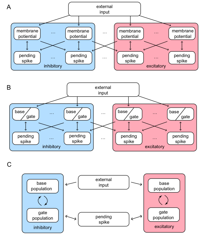
Figure 1: Structures and important features of 3 models. A. The structure of the full Markovian integrate-and-fire network. B. The structure of the reduced network model, where the membrane potentials only take values in $\{\mbox{Base, Gate}\}$. C. The structure of coarse grained model. In this model the pending $E$-kick pools for every neuron are merged in to one for the whole network, and so are the pending $I$-kick pools.

3 Results

In spiking neuronal networks, gamma frequency oscillations appear as temporally repeating, stochastic spiking clusters in the firing patterns. Different mechanisms have been proposed to explain this phenomena. As a minimal mechanism, interneuron network gamma (ING) proposes that the gamma oscillations can be produced by the fast interactimodelingons between inhibitory ($I$) neurons alone whittington2000inhibition (78). When inhibitory neurons have intrinsic firing rates higher than the gamma band, they may exhibit gamma firing frequency when mutually inhibited. ING does not require the existence of excitatory ($E$) neurons but studies showed that it loses its coherence in systems where neurons are heterogeneously driven wang1996gamma (76). Another class of theories view the repeating collective spiking clusters as the outcome of competition between $E$ neurons and $I$ neurons, such as the pyramidal-interneuron network gamma (PING, whittington2000inhibition (78, 9)) and recurrent excitation-inhibition (REI, chariker2018rhythm (19)).

Though sharing many common qualitative features, PING and REI provide substantially different explanations to the formation of gamma oscillations. Most remarkably, the collective spiking clusters in PING are usually whole-population spikes as a result of steady external input. The $E$-population spikes induce $I$-population spiking activities that are offset in time, and strong enough to suppress the entire network. A new $E$-population spiking event occurs after the inhibition wears off, leading to a series of nearly periodic, whole-population oscillatory activity.

On the other hand, the REI mechanism depicts a highly stochastic network dynamics: Driven by noisy stimulus, a few $E$-neurons crosses the threshold, and the subsequent recurrent excitation recruit more spikes from other excitatory neurons, leading to rapidly rising spike clusters. But this can not go forever since a few of the inhibitory neurons are excited at the same time, pushing the whole population to a less excitable condition. The next collective spiking event then emerges from the victory of excitation during its competition with inhibition. Therefore, the important features of the transient spike clusters are highly temporally variable, and the gamma frequency band of the oscillation is mainly a statistical feature of the emergent complex temporal firing patterns.

Our primary goal is to provide a better understanding of the emergence of gamma oscillations from the interaction between neurons in this nonlinear, stochastic, and high-dimensional context. In general, the biggest difficulty of analyzing spiking network dynamics is its dimensionality. Consider a network of $N$ neurons, the number of possible states grows exponentially as $N\to\infty$, no matter if we use a single-neuron model as complex as the Hodgkin-Huxley hodgkin1952quantitative (37) or as simple as binary-state cowan1991stochastic (24). Previously, many attempts have been made for model reduction by capturing collective network dynamics in specific dynamical regimes. Successful examples include kinetic theories CaiKinetic2006 (17) for mean-field firing patterns, statistical field theories buice2013beyond (14) for higher-order correlations, Wilson-Cowan neural field model wilson1972excitatory (79, 80) for spatial-temporal patterns, to name a few. In this study, our reduced models are developed with similar motivations to capture gamma oscillations. Generally, models incorporating many biologically realistic details can be very complicated; The reduced models are much easier to analyze, but some of the neglected information can lead to biases in many aspects. Here, we aim for a balance between realism and abstraction. Specifically, we present a sequence of reduced models, between which the connections are well defined (and can be mathematically analyzed in future studies). Importantly, we find that even the coarsest model preserves important features and statistics of the gamma oscillations found in the full model.

Our reduced models are based on the integrate-and-fire (IF) model, which is widely employed in previous models of spiking networks (see Methods). In a recent study, gamma oscillations have been found emerging from the simulation of a large-scale IF network model of layer 4C$\alpha$ of V1 chariker2018rhythm (19). Later theoretical studies suggest that gamma oscillations in different spatial regions decorrelate quickly on the scale of a couple of hypercolumns, echoing experimental observations that gamma oscillation is very local in cortex goddard2012gamma (33, 42, 52). Therefore, we first focus on a small homogeneous network with 75 excitatory neurons ($E$) and 25 inhibitory neurons ($I$) as an analogy of an orientation-preference domain of a hypercolumn in V1.

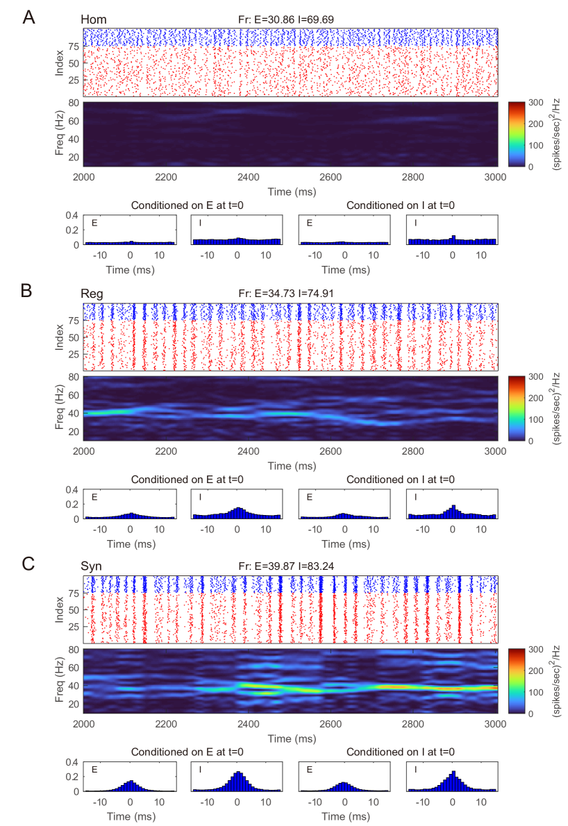
Figure 2: Gamma oscillation exhibited by the MIF network in three different regimes. A. Homogeneous regime (“Hom”). Top: Raster plots of all 75 $E$-neurons (blue) and $I$-neurons (red) with firing rates noted in title. Middle: The spectrogram of the firing pattern exhibiting low density in the gamma band (30-80 Hz). Bottom: The spiking correlation diagrams for $\{E,I\}$-spikes. B and C. Same as A. The regular (“Reg”) and synchronized (“Syn”) regimes exhibit much more synchronous firing patterns and stronger gamma-band activity.

3.1 Reduced Models Captures Statistics of Gamma Oscillations

3.1.1 A Markovian Intergrate-and-Fire network

We start with the Markovian integrate-and-fire model (MIF) first proposed in li2019well (43), and hereafter referred to as the “full model.” As an analogy of the conventional IF model (see Methods), the MIF brings us two additional conveniences: First, the discretized states of Markovian dynamics make theoretical analysis easier as the probability flow from one state to another is now straightforward; Second, the Markov properties of the MIF enable the computation of the invariant measure of gamma oscillations directly from the probability transition matrix.

Our MIF model network is composed of 100 interacting neurons (75 $E$-neurons and 25 $I$-neurons) driven by external Poissonian stimulus (Fig. 1A). The state of neuron $i$ is described by three variables $(v_{i},H^{E}_{i},H^{I}_{i})$, where $v_{i}$ represents individual membrane potentials and $H^{\{E,I\}}_{i}$ are analogies of the $E$ and $I$ conductances (see below). We use the size of external kicks to discretize the membrane potential, and let $v_{i}$ range from $V^{I}=-66$, the reversal potential of inhibitory synapses, to $V^{th}=100$, the spiking threshold. Immediately after reaching $V^{th}$, $v_{i}$ enters the refractory state $\mathcal{R}$, and, at the same time, sends a spike to its postsynaptic targets. After an exponentially distributed waiting-time $\tau^{\mathcal{R}}$, $v_{i}$ resets to the rest potential $V^{r}=0$. The ‘integrate’ part of MIF is separated into two components, external and recurrent. Each external kick increases $v_{i}$ by 1. To model the effects of recurrent network spikes, we use $H^{\{E,I\}}_{i}$ to denote the number of postsynaptic spikes (forming ‘pools’ of pending-kicks) received by neuron $i$ that has not yet taken effect. When receiving an ${\{E,I\}}$-spike, the corresponding pending-kick pool, $H^{\{E,I\}}_{i}$, increases by 1. Each postsynaptic spike affects $v_{i}$ independently, and after an exponentially distributed waiting-time (i.e., the synaptic time-scale) $\tau^{\{E,I\}}$, increase or decrease $v_{i}$ (depending on $\{E,I\}$ of the presynaptic neuron). The specific increment/decrement depends on the synaptic strength and the state of $v_{i}$. The connections between neurons are homogeneous: Whether a spike released by neuron $i$ is received by neurons $j$ is determined by an independent coin flip, whose probability only depends on the type of neuron $i$ and $j$. We leave the details and choices of parameters to Methods.

This 100-neuron MIF network exhibits gamma-band oscillations as demonstrated in li2019well (43) (Fig. 2). By varying the synaptic time scales $\tau^{\{E,I\}}$, we examine three regimes with different degrees of synchrony: homogeneous (“Hom”), regular (“Reg”), and synchronized (“Syn”). (Specifically, we fix the expectation of the waiting time for $I$-kicks ($\tau^{I}$) and manipulate separately the expectation of waiting time for $E$-spikes on $E$ and $I$ neurons, $\tau^{EE}$ and $\tau^{IE}$; for full details, see Methods). In the raster plot of “Hom” regime, the MIF network produces a firing pattern in which spikes do not exhibit strong temporal correlations (Fig. 2A top). (This is also verified by the spike-time correlations conditioned on each $\{E,I\}$-spike; see Fig. 2A bottom). Meanwhile, no strong spectral density peak is seen in the spectrogram (Fig. 2A middle). In the “Reg” regime, however, spikes begin to cluster in time as multiple firing events (hereafter, MFEs) and exhibit stronger spike-time correlations RanganYoung2013a (57, 58). Namely, MFE is a temporally transient phenomenon lying between homogeneity and total synchrony, where a part (but not all) of the neuronal population fires during a relatively short time window, as widely reported in previous experimental and modelling studies beggs2003neuronal (7, 21, 55, 64, 85, 86). Affected by MFEs, the mass of the spectral density is primarily located in the gamma band, especially around 40-60 Hz (Fig. 2B). Many more and stronger synchronized firing patterns, higher spike-time correlations, and stronger gamma-band spectral peaks are observed in the “Syn” regime. These dynamics and statistics are consistent with the results of li2019well (43) and in IF neuronal network simulations ZhangNewhallEtAl2014 (87, 88, 89). Furthermore, the gamma-band spectrograms are comparable with experimental studies xing2012stochastic (84).

We note that although our MIF network only consists of $N=100$ neurons, the number of states in the Markov chain is $(168\cdot n_{H^{E}}\cdot n_{H^{I}})^{N}$, where $n_{\{H^{E},H^{I}\}}$ are the largest possible sizes of the pending spike pools (see Methods for precise definition). Therefore, it is computationally unrealistic to do any meaningful analytical work to understand the dynamics, especially how gamma oscillations can emerge from the probability flows between different states. Therefore, we regard this MIF network as the “full model,” and apply dimensional reduction methods for further analysis.

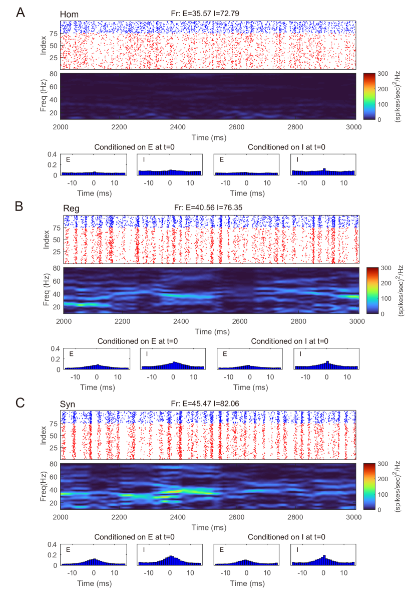
Figure 3: Gamma oscillation captured by the reduced network consisting of two-state neurons. A-C. Same regimes and statistics investigated in Fig. 2.

3.1.2 A Reduced Network with Two-State Neurons

First, we introduce a reduced network (RN) consisting of two-state neurons, i.e., RN model has the same setup as the MIF network except that the membrane potentials only have two states: base and gate (Fig. 1B). From the perspective of the full model, a neuron is deemed as a base or gate neuron by how far it is away from firing. Specifically, we set a cutoff $V^{c}$ below the threshold $V^{th}$, and neuron $i$ is regarded as a gate neuron if $v_{i}>V^{c}$, otherwise it is a base neuron (including $v_{i}\leq V^{c}$ and $v_{i}=\mathcal{R}$). Neuron $i$ flips between the base and gate states when

1. $v_{i}$ crosses the cutoff $V^{c}$, or

2. Neuron $i$ fires and enters the refractory state $\mathcal{R}$.

However, the reduction to two-state neurons immediately raises a question: Without the consecutive discrete states between $[V^{I},V^{th}]$, how can we represent the effect of (external, $E$/$I$-) kicks on individual neurons when $v_{i}$ only takes two possible states?

Consider an $E$-neuron $i$ in the gate state, i.e., $v_{i}>V^{c}$ in the corresponding MIF network. Since we do not know the exact value a priori, $v_{i}$ can take any value between $[V^{c},V^{th}]$ with a probability determined by the empirical distribution of the whole $E$-population. When an $E$-kick takes effect and increases $v_{i}$ by a synaptic strength of $S_{EE}$, neuron $i$ fires and changes state to “base” if and only if $v_{i}$ locates at the excitable region $(V^{th}-S_{EE},V^{th}]$, otherwise it stays in the gate state (and $v_{i}\in[V^{c},V^{th}-S_{EE})$). Therefore, a single $E$-kick has a probability

$$P_{E}^{GE}=\mathbf{P}\left(v_{i}\in(V^{th}-S_{EE},V^{th}]|v_{i}\in(V^{c},V^{th}]\right)=\frac{\mathbf{P}(v_{i}\in(V^{th}-S_{EE},V^{th}])}{\mathbf{P}(v_{i}\in(V^{c},V^{th}])},$$ (1)

to excite a gate $E$-neuron, leading to its spike and transition to the base state. That is, $P_{E}^{GE}$ is the transition probability of neuron $i$ in the excitable region, conditioned on that neuron $i$ is a gate neuron. A priori, we do not have the full distribution of neuronal states, therefore, in order to close the RN model, we use statistical learning methods by inferring $P_{E}^{GE}$ from a long-term simulation of the full MIF network. Likewise, we acquire all other transition possibilities induced by kicks (see Methods).

This reduction of classifying spiking neurons into two states is based on one simple assumption: The emergence of MFEs in the collective dynamics is mostly sensitive to one variable, i.e., the number of subthreshold neurons are only a few spikes from firing (gate neurons). On the other hand, the distribution of neurons with lower membrane potentials (base neurons) is less immediately relevant since it is much less possible for them to generate spikes in the next few milliseconds. Therefore, the initiation and maintenance of gamma oscillations are dominated by the probability flow between gate and base states.

Even with such a drastic simplification, the RN model provides remarkably good approximation of dynamics produced by the MIF network (Fig. 3), which is verified by raster plots, firing rates, and spectrum densities similar to those of the full model in Fig. 2. On the other hand, we notice that the spike-time correlations in the “Syn” regime are indeed slightly lower than the corresponding value in the full model. This is not very surprising: When the spiking pattern is synchronized, the dynamics is more sensitive to the details of the probability distribution of neurons in the excitable region since one spike may trigger more spikes followed by other neurons. One may, of course, consider using more information to describe the full distribution of the membrane potentials (perhaps by using three or more states instead of two). Though a more detailed models may provide us with better numerical approximations, our primary goal of capturing the key features of gamma oscillation has been well served by the current version of the RN model with two-state neurons.

Though radically simplified, our RN model is still a Markov chain, with $(2\cdot n_{H^{E}}\cdot n_{H^{I}})^{N}$ states. However, the setup and success of the RN model provide important insights for further model reduction.

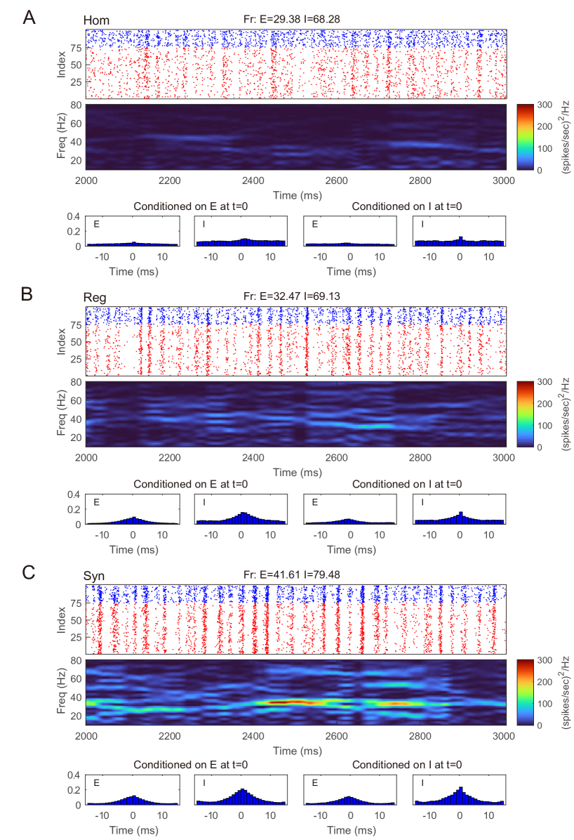
Figure 4: Gamma oscillation captured by the coarse-grained model. A-C. Same regimes and statistics investigated in Fig. 1 and 2. The fake raster plots are produced by randomly assigning spikes to each neuron.

3.1.3 A Coarse-Grained Approximation

When we infer the transition probabilities between gate and base states, we are uncertain of the full distribution of $v_{i}$ in the network (besides the number of neurons in base and gate states). Therefore, the success of the RN model suggests that we may think of the transition probabilities as functions of the number of $\{E,I\}$ neurons in each state: $N_{GE}$, $N_{GI}$, $N_{BE}$, $N_{BI}$. Thus, the core idea of further simplifying by coarse-grained (CG) approximation is this: Instead of thinking about the state of each individual neuron, we study the state of population statistics. Below we summarize the setup of our CG model and leave the details to Methods.

Let us first consider the pending-kick pools of a single neuron. Take the $I$-to-$E$ and $I$-to-$I$ projections as an example: Because of the homogeneity of the network, for an $I$-spike, each of its postsynaptic neuron receives it independently with a probability that depends only on the specific neuronal type $\{E,I\}$. In addition, each spike takes effect independently, with the same waiting time distribution (exponential with mean $\tau^{I}$). Therefore, this is equivalent to a collective $I$-kick pool of size $H^{I}$, representing the sum of all $I$-kick pools in the entire network. In this pool, each pending-kick takes effect independently and is randomly distributed to a specific neuron with a probability depending only on its $E/I$ type. With similar considerations, the $E$-kick pools are also merged into one at a size $H^{E}$. However, since $(\tau^{EE},\tau^{IE})$ are separately manipulated in the full model, we have to ignore the subtle differences between the consumption rates of pending $E$-kicks on $E$ and $I$ neurons. Specifically, we assume that a constant portion of $H^{E}$ are distributed to $E$ ($I$) neurons (i.e., $H^{EE}=a^{EE}\cdot H^{E}$. See Methods), which introduces a bias in our CG model.

Since each neuron is driven by the same, coarse-grained $\{E,I\}$-kick pools, due to the interchangeability of $I$ neurons, they are now only differentiated by their current state (base or gate). Similarly, the information of the state of every $I$ neuron is now represented by the Numbers $(N_{BI},N_{GI})$. Since the total number of $I$ neurons is fixed, we only need $N_{GI}$. These considerations also apply to the $E$ neurons. Thus, our CG model becomes a Markov chain with four variables:

$$(N_{GE},N_{GI},H^{E},H^{I}).$$ (2)

Kicks taking effect may change $N_{GE}$ and $N_{GI}$, and spikes released by neurons increase $H^{E}$ and $H^{I}$. The CG model contains $N_{E}\cdot N_{I}\cdot N_{H^{E}}\cdot N_{H^{I}}$ states ($N_{H^{E}}=n_{H^{E}}\cdot N$, $N_{H^{I}}=n_{H^{I}}\cdot N$). For each state, there are at most 12 possible transitions to other states (see Methods). Therefore, the CG model becomes an $O(N^{4})$ problem, allowing us to analyze the dynamics in detail.

The CG model is a natural simplification of the RN model, and it is reasonable to expect CG to capture the main features of gamma oscillations. Indeed, we find that in all three regimes we considered, the behaviors of CG model are in well agreement with both the MIF and RN models (Fig. 4). Note that, since we do not track the dynamics of individual neurons in CG, the (fake) raster plots are generated by randomly assigning spikes to neurons.

3.2 Gamma Dynamical Features in Reduced Models

The reduced models are not designed to reproduce every detail of the full model. But how well can our model reduction capture the dynamics and key statistical features? In addition to the firing rates, spectral densities, and spike-time correlations for the three selected regimes, we examine the RN and CG models when we change parameters continuously. In this section, we test two dynamical features observed in the full, MIF model. For each parameter set involved, we numerically simulate each of the three models (MIF, RN, and CG), for 10 seconds each, and divide the dynamics into 10 batches. We then show the batch means and standard errors of the statistics collected from the batches (Fig. 5).

First, when the frequency of the external Poisson stimulus ($\lambda$) increases, MFEs appear more frequently in the firing patterns. According to chariker2018rhythm (19), a new MFE is initiated by excitatory stimulation or by chance when the inhibition from the last MFE fades. Therefore, stronger external stimuli result in faster initiation of a new MFE. From the firing patterns of our three models, we use a spike cluster detection algorithm chariker2015emergent (20) to recognize individual MFEs (see Methods) and examine how their emergence is regulated by external stimulus. We find that the RN and CG models capture the same trend exhibited in the full model (Fig. 5A), namely, the average waiting time of MFE (1/MFE frequency) is linearly related to the external kicks ($\lambda^{-1}$). However, while the trend is captured semi-quantitatively, the reduced models exhibit lower MFE frequencies (or higher MFE waiting time in Fig. 5A, red and yellow). On the other hand, we find that the MFEs produced by the RN and CG models have longer duration than the MIF model (See Supplementary Materials). These results suggest that, on average, the reduced models have slower probability flows between states.

Second, when the ratio $\nicefrac{{\tau^{EE}}}{{\tau^{I}}}$ becomes smaller, the $E$-kicks take effect on $E$ neurons relatively faster, and thus, the recurrent network excitation recruits other $E$-spikes on a shorter time scale. Therefore, the whole network exhibits more synchronized firing patterns. This phenomena has been observed in many previous computational models (see, for instance, KeeleyEtAl2019 (39)), and also verified by the comparison between the three regimes in this paper. Here we go beyond these three regime and change $\tau^{EE}$ continuously while fixing $\tau^{I}$ (Fig. 5B). In the full model, the degree of synchrony (measured by spike synchrony index, see Methods) exhibits a clear decreasing trend when $\tau^{EE}$ goes up, which is also well-echoed by the RN model. For the CG model, however, although the same trend is captured, the degree of synchrony is generally higher than in the full model. This bias is introduced when we merge all $E$-kick pools into one and assume $\nicefrac{{H^{EE}}}{{H^{IE}}}$ is a constant: The underestimation of $H^{IE}$ delays the spikes of $I$ neurons and the MFEs are artificially prolonged, leading to higher synchrony. To verify this point, we carry out a CG model reduction with five variables $(N_{GE},N_{GI},H^{EE},H^{IE},H^{I})$ by keeping separately the pending $E$-kick pools of the $E$ and $I$ populations. In this five-variable CG model, the degree of synchrony is indeed much closer to the full model (see Supplementary Materials).

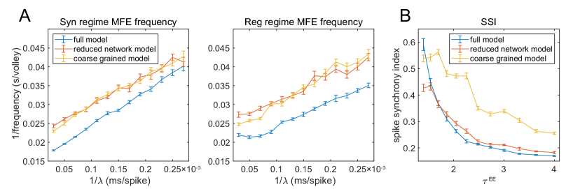
Figure 5: Two gamma features captured by reduced models. A. MFE waiting time linearly related to external stimulation waiting time. Left: Syn regime; Right: Reg regime. B. Degree of synchrony decreases when $\tau^{EE}$ increases.

3.3 Gamma Oscillations Remain Near a Low-Dimensional Manifold

Our most remarkable finding is that the emergent gamma oscillations in the full model stay near a low-dimensional manifold. Inspired by the fact that the gamma dynamics is successfully captured by the dynamics of only four variables, we simulate the full model in the “Syn” regime, and then project the trajectories onto the 4-dimensional state space suggested by the success of our CG model, i.e., we collect the statistics $(N_{GE},N_{GI},H^{E},H^{I})$ from the full model dynamics (Fig. 6A; see also Fig. 7A).

Since $N_{GE}$ and $N_{GI}$ are positively correlated (Fig. 6A, Middle; See also Fig. 7A, bottom panel), we examine the three-dimensional subspace of $(N_{GE},H^{E},H^{I})$. Strikingly, the full model trajectories suggest a low-dimensional dynamical structure of gamma oscillations. This observation is also verified by the mass estimation from the trajectories collected from a long-time (50s) simulation of the full model (Fig. 6B). On the other hand, we also simulate the CG model for 10 seconds and find similar trajectories in state space (Fig. 6C), accounting for its successful reproduction of the emergent gamma dynamics. Since the CG model only consists of $O(N^{4})$ states, its invariant probability distribution becomes computable from the Markov transition probabilities matrix. Here we present the mass of the distribution after we further “shrink” the CG model and reduce the number of states to millions (Fig. 6D. See Methods for the “shrunk” CG model). The invariant probability distribution not only displays similar mass of density as the full model, but on which the trajectories of the full model remain near (See Supplementary Materials).

The trajectories and the probability distributions of both the full MIF and corresponding CG models reveal a two-dimensional manifold structure with a certain thickness in the orthogonal direction (Fig. 6A-D). To verify this point, we carry out a local dimensionality estimation of the full model data (see Methods). Notably, the manifold exhibits a nearly two-dimensional local structure at most of the places (Fig. 6E, cyan and green parts), except for a region with low $H^{E},H^{I}$ and low-to-medium $N_{GE}$ (Fig. 6E, red part. $0<N_{GE}<30$, $H^{E}<20$, $H^{I}<200$). The regions with high dimensionality correspond to the inter-MFE periods (where both number of gate neurons and pending kick pools are small, $0<N_{GE}<15$) and the initiation of MFEs (where $15<N_{GE}<30$). This is not very surprising: Inter-MFE periods are highly affected by the external stimuli, and the size of each MFE depends on how many $E$-neurons are recurrently recruited by the $E$-spikes at the very beginning. Both processes are highly stochastic, resulting into higher dimensionalities. We note that, this local two-dimensional structure is also verified by the results of local linear embedding (LLE). When we apply LLE to the 10-second full model trajectories (from four-dimensional to three-dimensional), they display a two-dimensional manifold as well, in the three-dimensional LLE space (Fig. 6F).

The trajectories of the MIF model give us a clear view of the temporal organization of the emergent gamma dynamics. First of all, we observed that $(N_{GE},N_{GI})$ are strongly positively correlated (Fig. 7A, bottom panel), although $N_{GI}$ rises slightly faster than $N_{GE}$ at the initiation of each MFE. In other words, the probability flow of membrane potential distribution of $E$ and $I$ populations are mostly temporally synchronized, which is also observed in previous computational models RanganYoung2013a (57, 89, 19). In the three-dimensional subspace of $(N_{GE},H^{E},H^{I})$, the low-dimensional manifolds help us interpret the gamma dynamics as follows:

1. At the beginning of each MFE, due to the external stimulus and faded recurrent inhibition, the membrane potentials moves up (represented by increasing $(N_{GE},N_{GI})$. Fig. 6A-D, Middle). Note that $N_{GI}$ moves up slightly faster due to the lower $I$-to-$I$ connectivity compared to $I$-to-$E$.

2. Some $E$ neurons fire, possibly eliciting more spikes from other $E$ neurons, so $H^{E}$ increases fast during this phase.

3. $I$ neurons are excited by $H^{E}$ at the same time, and $H^{I}$ increases as well. Note that $H^{E}$ is always consumed faster due to smaller $\tau^{E}$. In this phase, $H^{E}$ attains its peak while $H^{I}$ still increases rapidly.

4. $H^{E}$ is then consumed and the system is now dominated by the inhibition brought by $H^{I}$ leading to the end of the MFE. High $H^{I}$ brings down $(N_{GE},N_{GI})$, and terminating the MFE, leading to the inter-MFE-period. The next MFE is unlikely to start until $H^{I}$ is mostly consumed.

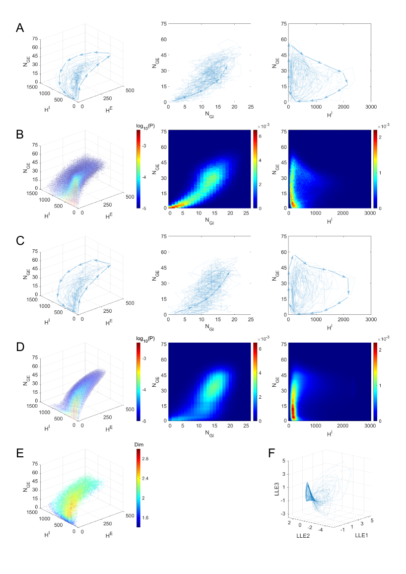
Figure 6: Gamma dynamics restricted on a low-dimensional manifold. A. The trajectories of the full model (Syn regime) presented the state space $(N_{GE},N_{GI},H^{E},H^{I})$. Left: The projection on subspace $(N_{GE},H^{E},H^{I})$; Middle: The projection on subspace $(N_{GE},N^{GI})$; Right: The projection on subspace $(N_{GE},H^{I})$. B-D depict the same subspaces as A. B. Mass of trajectory density of the full model. C. The trajectories of the CG model (Syn regime). D. The stationary probability distribution of CG model. E. Local dimensionality of data for the full model trajectories, displayed in the same view as A. F. The full model trajectories are local linearly embedded in a three-dimensional space.

4 Discussion

The vast range of observed neuronal network dynamics presents a tremendous challenge to systems neurophysiologists, data analysts, and computational neuroscientists. Evermore detailed neurophysiological datasets and large-scale neuronal network simulations reveal dynamical interactions on multiple spatial and temporal scales that also participate in essential brain functions. The observed dynamics exhibits rapid, stochastic fluctuations incorporating strong, transient correlations, quite possibly leading to its complexity. Unfortunately, the emergent fluctuating activity cannot effectively be described by standard ensemble averages, as many population methods cannot capture many of the low order statistics associated with the observed dynamical regimes.

The diversity and hierarchy of experimentally observed dynamics in the brain poses this immediate question: What concise, unified mathematical framework can reproduce the co-existence of transient, heterogeneous dynamical states, emerging from a high-dimensional, strongly recurrent neuronal network. Here we focus on gamma frequency oscillations because of their role underlying the transient fluctuations within the stationary states of complex neuronal networks (see, for instance, SiegelDonnerEngel2012 (65, 16)), and the belief that they are significant contributors to neural information processing Fries2009 (29, 75).

Important theoretical progress has been made by coarse graining sparsely coupled networks (see, for instance, BrunelHakim1999 (13, 17), and references therein). These approaches were able to capture spatio-temporal network dynamics dominated by mean-field and uncorrelated synaptic fluctuations. Also influential were the studies focusing on weakly-coupled oscillators. Recent work has made significant theoretical advances by mapping populations of the quadratic IF neurons and the so-called theta neurons to systems of Kuramoto oscillators MontbrioEtAl2015 (53, 41), where the tools of phase oscillator theory ashwin2016mathematical (1, 8) can be used to give insight into network synchronization. We view our approach here as complementary to these studies.

Here we demonstrate that, by starting with a Markovian IF model, we can bring the tools of classical Markov processes to bear on stochastic gamma oscillations. Using a model first studied by li2019well (43), we show that we can dimensionally reduce and coarse-grain the model network, first, to a two-state reduced network model and then, to a model of transition probabilities between the number of neurons in the two-state, reduced model. The full repertoire of network dynamics between homogeneity and synchrony is faithfully reproduced by our reduced models. Furthermore, by preserving the Markovian dynamics at each step, and combining with data-driven approaches, we were able to reveal locally two-dimesionaly invariant manifolds underlying the type of gamma oscillations observed in large-scale numerical simulations.

A tremendous amount of experimental and theoretical literature implicates oscillatory, coherent neural activity as a crucial element of cognition. Here we provided a simple framework through which collective behavior of populations of neurons can be coarse-grained to counting statistics of neurons in specific neuronal states. This dynamical perspective not only can afford a concise handle for the systems neuroscientists, with experimental access to neuronal circuits and populations, but also to the theoreticians, who may wish to build computational and information processing frameworks on top of these coarse-grained, low-dimensional representations.

While we have detailed our methodology for a system with a small number of neurons and homogeneous connectivities, preliminary studies show that we can scale up to much larger networks (see Supplementary Information). We can extend our framework to networks with slowly varying spatial inhomogeneities (e.g., V1 orientation hypercolumns coupled by long-range excitatory connections) and in capturing interneuronal correlations in predominantly feedforward networks, like synfire chains DiesmannEtAl1999 (26, 77, 83), with each local, nearly homogeneous population described by CG modules (of 2-3 states plus the relevant pending-spike pools). At the same time, we are examining data-driven and machine learning approaches to estimate the various states and transition probabilities directly from numerical simulations, with the hope of applying to neurophysiological data sets. Finally, we are already looking to incorporate higher-order structural motifs in the network connectivity. Higher-order motifs SongEtAl2005 (69) are likely to substantially influence the types of dynamical correlations within complex networks, and consequently, activate a multitude of spatio-temporal spiking patterns that may have important consequences for information processing and coding in the mammalian brain zhao2011synchronization (90, 38).

Methods

Integrate-and-Fire Network

Consider an $N$-neuron Integrate-and-Fire (IF) neuronal network with $N_{E}$ excitatory neurons ($E$) and $N_{I}$ inhibitory neurons ($I$), where the membrane potential ($v_{i}$) of each neuron is driven by a sum of synaptic currents:

$$\begin{split}\frac{{\rm d}{v_{i}}}{{\rm d}t}&=\left(g_{i}^{ext}+g_{i}^{E}\right)\cdot\left(V^{E}-v_{i}\right)+g_{i}^{I}\left(V^{I}-v_{i}\right),\\ g_{i}^{ext}&=S_{i}^{ext}\sum_{\mu_{i}^{ext}}G^{E}(t-t_{\mu_{i}^{ext}}),\\ g_{i}^{E}&=\sum_{\begin{subarray}{c}j\in E\\ j\neq i\end{subarray}}S_{ij}^{E}\sum_{\mu_{j}^{E}}G^{E}(t-t_{\mu_{j}^{E}}),\qquad g_{i}^{I}=\sum_{\begin{subarray}{c}j\in I\\ j\neq i\end{subarray}}S_{ij}^{I}\sum_{\mu_{j}^{I}}G^{I}(t-t_{\mu_{j}^{I}}),\end{split}$$ (3)

where $g_{i}^{\{ext,E,I\}}$ are the external, excitatory and inhibitory conductances of neuron $i$. Each neuron receives excitatory spiking stimulus from an external source ($\mu_{i}^{ext}$) and other excitatory/inhibitory neurons in the network $\mu_{j}^{\{E,I\}}$, where the strength of synaptic couplings are represented by $S_{i}^{ext}$ and $S_{ij}^{\{E,I\}}$, respectively. A spike is released by neuron $i$ when its membrane potential $v_{i}$ reaches the threshold $V^{th}$. After this, neuron $i$ immediately enters the refractory period, and remains there for a fixed time of $\tau^{\mathcal{R}}$ before resetting to rest $V^{r}$. It is conventional in many previous studies to choose $V^{th}=1$ and $V^{r}=0$ CaiKinetic2006 (17). Accordingly, $V^{E}=\nicefrac{{14}}{{3}}$ and $V^{I}=-\nicefrac{{2}}{{3}}$ are the excitatory and inhibitory reversal potentials. Each spike changes the postsynaptic conductance with a Green’s function,

$$\begin{split}G^{E}(t)&=\frac{1}{\tau^{E}}e^{-\nicefrac{{t}}{{\tau^{E}}}}h(t),\\ G^{I}(t)&=\frac{1}{\tau^{I}}e^{-\nicefrac{{t}}{{\tau^{I}}}}h(t),\end{split}$$ (4)

where $h(t)$ is the Heaviside function. The time constants, $\tau^{\{E,I\}}$, model the time scale of conductances of the excitatory and inhibitory synapses (such as AMPA and GABA gerstner2014neuronal (32)).

While Eq. (3) can model a network with arbitrary connectivity structure, in this paper, we focus on homogeneous networks. That is to say, whether certain spike released by a neuron of type $Q$ is received by another neuron of type $Q^{\prime}$ is only determined by an independent coin flip with a probability $P_{Q^{\prime}Q}$, where $Q,Q^{\prime}\in\{E,I\}$. Furthermore, $S_{ij}^{\{E,I\}}$ are also considered as constants independent of $i,j$.

Three different levels of models are illustrated below. The Markovian integrate-and-fire network approximates Eq. (3) with a Markov process, and the following reduced network and coarse-grained model are reductions of the full Markovian model.

Full Model: A Markovian Integrate-and-Fire Network

Following a previous study li2019well (43), we rewrite Eq. (3) as a Markov process to facilitate theoretical analysis. Therefore, we need to minimize the effects of the memory terms and discretize membrane potentials and conductances. Specifically, $v_{i}$ takes values in

$$\Gamma:=\left\{V^{I},V^{I}+1,\ldots,V^{r}-1,V^{r},V^{r}+1,\ldots,V^{th}\right\}\cup\{\mathcal{R}\},$$ (5)

To be consistent with the IF network (3), we choose $V^{I}=-66$, $V^{r}=0$, and $V^{th}=100$. As before, $v_{i}$ enters the refractory state $\mathcal{R}$ immediately after reaching $V^{th}$. However, in this Markovian IF (MIF) network, the total time spent in $\mathcal{R}$ is no longer fixed, but an exponential-distributed random variable $\tau^{\mathcal{R}}$.

Each neuron receives the external input as an independent Poisson process with rate $\lambda_{\{E,I\}}$, and $v_{i}$ goes up for 1 when an external kick arrives. On the other hand, the synaptic conductances of each neuron $g_{i}^{\{E,I\}}$ are replaced by “pending-kick pools,” $H_{i}^{\{E,I\}}$. Consider excitatory spikes as an example: Instead of updating $g_{i}^{E}$ with Green’s functions when neuron $i$ receives an $E$-spike, we add the new spike to an existing spike pool $H_{i}^{E}$. Each spike in the pool will affect $v_{i}$ independently after an exponentially-distributed waiting time $\tau^{E}$. $H_{i}^{E}$ is the number of spikes has not taken effect yet. Therefore, for the a sequence of $E$-spikes received by neuron $i$, it is not hard to see that $\mathbb{E}[H_{i}^{E}(t)]=\mathbb{E}[g_{i}^{E}(t)]$.

How each spike changes $v_{i}$ is determined by the type of the spike ($Q^{\prime}$), the type of neuron $i$ ($Q$), and the state of $v_{i}$. When a spike takes effect, the membrane potential stays unchanged if $v_{i}=\mathcal{R}$, otherwise $v_{i}$ may jumps up (for an $E$-spike) or down (for an $I$-spike). On the other hand, the size of each jump depends on the membrane potential, $v_{i}$, and the synaptic coupling strengths, $S_{QQ^{\prime}}$. For an $E$-spike, $v_{i}$ increases by $S_{QE}$. For an $I$-spike, however, the size of the decrement is $\nicefrac{{(v_{i}-V^{I})}}{{(V^{th}-V^{I})}}\cdot S_{QI}$. The difference in the effects of $\{E,I\}$-spikes is due to the relative values of the reversal potentials. The currents induced by $g_{i}^{I}$ is sensitive to $v_{i}$ while the currents induced by $g_{i}^{E}$ is much less sensitive, i.e., in Eq. (3):

$$0\leq|v_{i}-V^{I}|\leq\frac{5}{3},\quad\frac{11}{3}\leq|v_{i}-V^{I}|\leq\frac{16}{3}$$ (6)

In our MIF network, we take most of the system (synaptic and stimulus) parameters directly from li2019well (43), but modified a few to accommodate the smaller network studied here ($N_{E}=75$ vs. $N_{E}=300\sim 1000$ in li2019well (43)). The parameters are summarized below:

• Frequencies of external input: $\lambda_{E}=\lambda_{I}=7000$ Hz;

• Synaptic strength: $S_{EE}=S_{EI}=S_{II}=20$, and $S_{IE}=8$;

• Probability of spike projections: $P_{EE}=0.15$, $P_{IE}=P_{EI}=0.5$, and $P_{II}=0.4$;

• Synaptic time-scales: $\tau^{I}=4.5$ ms. $\tau^{E}<\tau^{I}$ to reflect the fact that AMPA is faster than GABA. We use different choices of $\tau^{E}$ for regimes implying different dynamics (all indicated in ms):

  1. Homogeneous (“Hom”): $\tau^{EE}=4$, $\tau^{IE}=1.2$,

  2. Regular (“Reg”): $\tau^{EE}=1.7$, $\tau^{IE}=1.2$,

  3. Synchronized (“Syn”): $\tau^{EE}=1.4$, $\tau^{IE}=1.2$,

Reduced Network Consisting of Two-State Neurons

The reduced network (RN) is a direct reduction of the MIF network by reducing the size of the state space for membrane potentials. In RN, each neuron $i$ is a two-state neuron flipping between “base” or “gate” states, i.e., instead of taking values in the state space $\Gamma$, now $v_{i}\in\Gamma_{2}=\{B,G\}$. A neuron in the MIF network is deemed “base” or “gate” depending on how likely it is going to fire in the next couple of millisecond: Consider a certain cutoff $V^{c}\in\Gamma$, neuron $i$ is a gate neuron if $v_{i}\geq V^{c}$ since it is closer to the threshold and is only a couple of $E$-kicks away from spiking. Otherwise, neuron $i$ is a base neuron if $v_{i}<V^{c}$ or $v_{i}=\mathcal{R}$. Therefore, a flip from base to gate can take place when an $E$-spike or external stimuli takes effect and $v_{i}$ crosses $V^{c}$ from the lower side; on the other hand, a flip from gate to base may be due to $v_{i}$ crossing $V^{c}$ from the higher side when 1) an $I$-spike takes effect, or 2) the neuron fires and enters the refractory period.

The network with two-state neurons is reduced from the MIF network by combining states together, but generally we do not expect the full MIF model as a lumpable Markov process tian2006lumpability (71). Therefore, the appropriate transition probability between the base and gate states should be carefully estimated so that the RN can correctly capture the dynamics of the MIF network. Since the flip between states can only take place after certain spikes, the possibilities are:

• Effect of external stimuli: When a kick arrives, a base $\{E,I\}$ neuron will become a gate $\{E,I\}$ neuron with probability $\{P_{ex}^{BE},P_{ex}^{BI}\}$, while a gate $\{E,I\}$ neuron will fire and become a base $\{E,I\}$ neuron with probability $\{P_{ex}^{GE},P_{ex}^{GI}\}$.

• Effects of E-kicks: Similar types of transitions here but different probabilities due to different sizes of kicks: $\{P_{E}^{GE},P_{E}^{GI},P_{E}^{BI},P_{E}^{BE}\}$.

• Effects of I-kicks: The I-kicks do not have any effect on a base neuron. But I-kicks will depress a gate neuron to a base neuron with probabilities $\{P_{I}^{GE},P_{I}^{GI}\}$.

All transition probabilities listed above are time-dependent and determined by the distribution of membrane potentials of neurons in the network. As a first approximation, we can collect their statistics from a long-time simulation of the MIF network. Here we illustrate how to compute $P_{E}^{BE}$ for example, and everything else follows. Consider the distribution of membrane potentials of $E$-neurons, $p_{E}(v)$. Then $P_{E}^{BE}$ is the conditional probability a base $E$-neuron goes across $V^{c}$ within one $E$-kick, which is expressed as:

$$P_{E}^{BE}\left\{p_{E}\right\}=\frac{\int_{V^{c}-S_{EE}}^{V^{c}}p_{E}(v)\,\mbox{d}v}{\int_{v<V^{c},v=\mathcal{R}}p_{E}(v)\,\mbox{d}v}$$ (7)

However, in RN, we do not see the exact distribution $p_{E}(v)$, but only the number of base and gate $E$-neurons ($N_{GE},N_{BE}$) instead. Therefore, to set a closure condition for RN, we consider $P_{E}^{BE}$ as a function of $N_{BE}$ regardless of the specific distributions, i.e.,

$$\overline{P_{E}^{BE}}(N_{BE})=\operatorname{E}\left[P_{E}^{BE}\left\{p_{E}\right\}\nonscript\;\middle|\nonscript\;\int_{v<V^{c},v=\mathcal{R}}p_{E}(v)\,\mbox{d}v=\frac{N_{BE}}{N_{E}}\right]$$ (8)

Finally, to collect $\overline{P_{E}^{BE}}(N_{BE})$, we run the MIF network simulations for a long time and collect all the events when a $E$-kick takes effect and the membrane potential distribution satisfies the condition listed above. The estimate of $\overline{P_{E}^{BE}}(N_{BE})$ is hence the probability of one base $E$-neuron crossing $V^{c}$ conditioned on these events.

Readers should note that, the three regimes (Hom, Reg, and Syn) investigated in this paper are only differentiated in the waiting time of kicks, i.e., the transition probabilities induced by single kicks are similar, given the observation that the subthreshold distributions in these regimes are alike. Therefore, to carry out reduction in these regimes, we only need the simulation of one canonical parameter set (say Syn) rather than all of them.

A Coarse-Grained Approximation

A coarse-grained (CG) approximation is developed to further reduce the number of states of the network. The MIF network has $O((168\cdot n_{H}^{2})^{N})$ states, where $n_{H}$ is the largest possible number of pending kicks for a neuron. The number for the RN is lower, as $O((2\cdot n_{H}^{2})^{N})$, and yet it still grows exponentially with the size of the network. This number is already astronomical for the 100-neuron network studied in this paper.

A CG approximation of RN model is carried out as follows:

• First of all, due to the homogeneous connectivity of the network, all $I$-neurons have the same probability to add an $E$-kick to their pending-kick pools when an $E$-neuron $i$ fires. Since each kick takes effect independently, this is equivalent to a large pool containing all $E$-kicks of the $I$-neurons and each $E$-kicks are randomly distributed to a specitic $I$-neuron. Therefore, we only need the size of the large pool $H^{IE}$ rather than individual $E$-pending-kick pools for each $I$ neuron. Likewise, we have pools $H^{EE}$, $H^{EI}$, and $H^{IE}$ for other pending spikes. (Note that this CG simplification does not rule out autapses, i.e., the possibility that a spike takes effect on the neuron releasing it. This may be an issue when the network is very small; however, it does not cause any obvious problems in our model with 100 neurons.)

• We now try to further combine the pools. Since all $I$-kicks are consumed with the same waiting time $\tau^{I}$, we can combine the two $I$-kick pools together. This does not directly apply to the two $E$-kick pools since $\tau^{EE}\neq\tau^{IE}$, and bias is introduced when we combine $H^{EE}$ and $H^{IE}$, since they are consumed at different rates. We have to assume two constants $a^{EE}+a^{IE}=1$, where

  $$H^{EE}=a^{EE}\cdot H^{E},\quad H^{IE}=a^{IE}\cdot H^{E},$$ (9)

  On the other hand, $\tau^{EE}$ and $\tau^{IE}$ are closer in the Syn regime, i.e., $\nicefrac{{H^{EE}}}{{H^{IE}}}\approx\mbox{const}$ and the introduced bias is smaller in this regime (Fig. 7A). In all,

  $$H^{E}=H^{EE}+H^{IE}=\sum_{i=1}^{N}H_{i}^{E},\quad H^{I}=H^{EI}+H^{II}=\sum_{i=1}^{N}H_{i}^{I},$$ (10)

  where $H^{\{E,I\}}$ are the sizes of the $\{E,I\}$-kick pools for the whole network.

• Finally, by definition, the transition probabilities of the two-state neurons are functions of the number of gate neurons (see Eq. 8). Therefore, instead of the states of each individual neuron, the distributions of membrane potentials can be determined by the numbers of gate neurons $(N_{GE},N_{GI})$. Once they are computed, the number of base neurons is given by

  $$N_{GE}+N_{BE}=N_{E},\quad N_{GI}+N_{BI}=N_{I}$$ (11)

Therefore, the CG approximation above is a Markov process with only four variables, two for the number of gate neurons and two for pending kicks $(N_{GE},N_{GI},H^{E},H^{I})$, and the number of states is $O(N^{4})=N_{E}\cdot N_{I}\cdot(n_{H})^{2}$. This is a tremendous reduction from exponential to polynomial scaling in the size of the network. We here provide a qualitative description of the dynamics of the coarse-grained model: When an $\{E,I\}$-kick takes effect, the number of $H^{\{E,I\}}$ minus one, and certain neuron flips between base/gate states with probability (represented by the change of $N_{GE},N_{GI}$); If an $\{E,I\}$-neuron fires, a spike is released and the pending-kick pool $H^{\{E,I\}}$ expands by

$$M_{E}=P_{EE}N_{E}+P_{IE}N_{I},\quad M_{I}=P_{EI}N_{E}+P_{II}N_{I},$$ (12)

where $M_{\{E,I\}}$ is the average number of postsynaptic neuron recipients of an $\{E,I\}$-spike.

We list all possible transitions from state $X=(N_{GE},N_{GI},H^{E},H^{I})$ (Table 1). In addition, since all state transitions are triggered by certain kicks, which take effect independently with exponential waiting time, it is more important to know the the transition rates based on the transition probabilities. We list these rates in Table 2.

external kick takes effect	one $E$-kick takes effect	one $I$-kick takes effect
$N_{GE}+1$	$N_{GE}+1\quad H^{E}-1$	$N_{GE}-1\quad H^{I}-1$
$N_{GI}+1$	$N_{GI}+1\quad H^{E}-1$	$N_{GI}-1\quad H^{I}-1$
$N_{GE}-1\quad H^{E}+M_{E}$	$N_{GE}-1\quad H^{E}-1+M_{E}$	$H^{I}-1$
$N_{GI}-1\quad H^{I}+S_{I}$	$N_{GI}-1\quad H^{E}-1\quad H^{I}+S_{I}$
Remain	$H^{E}-1$

Table 1: All possible transitions from state $X=(N_{GE},N_{GI},H^{E},H^{I})$ to another. There are 13 cases in all.

external kick takes effect	one $E$-kick takes effect	one $I$-kick takes effect
$P^{BE}_{ex}N_{BE}\cdot\lambda_{E}$	$P^{BE}_{E}a_{EE}\frac{N_{BE}}{N_{E}}H^{E}/\tau^{EE}$	$P^{GE}_{I}a_{EI}\frac{N_{GE}}{N_{E}}H^{I}/\tau^{I}$
$P^{BI}_{ex}N_{BI}\cdot\lambda_{I}$	$P^{BI}_{E}a_{IE}\frac{N_{BI}}{N_{I}}H^{E}/\tau^{IE}$	$P^{GI}_{I}a_{II}\frac{N_{GI}}{N_{I}}H^{I}/\tau^{I}$
$P^{GE}_{ex}N_{GE}\cdot\lambda_{E}$	$P^{GE}_{E}a_{EE}\frac{N_{GE}}{N_{E}}H^{E}/\tau^{EE}$	$(1-P^{GE}_{I}a_{EI}\frac{N_{GE}}{N_{E}}-P^{GI}_{I}a_{II}\frac{N_{GI}}{N_{I}})\cdot H^{I}/\tau^{I}$
$P^{GI}_{ex}N_{GI}\cdot\lambda_{I}$	$P^{GI}_{E}a_{IE}\frac{N_{GI}}{N_{I}}H^{E}/\tau^{IE}$
$\begin{aligned} &(1-P^{BE}_{ex})N_{BE}\cdot\lambda_{E}\\ +&(1-P^{BI}_{ex})N_{BI}\cdot\lambda_{I}\\ +&(1-P^{GE}_{ex})N_{GE}\cdot\lambda_{E}\\ +&(1-P^{GI}_{ex})N_{GI}\cdot\lambda_{I}\end{aligned}$	$\begin{aligned} &(1-P^{BE}_{E})a_{EE}\frac{N_{BE}}{N_{E}}H^{E}/\tau^{EE}\\ +&(1-P^{BI}_{E})a_{IE}\frac{N_{BI}}{N_{I}}H^{E}/\tau^{IE}\\ +&(1-P^{GE}_{E})a_{EE}\frac{N_{GE}}{N_{E}}H^{E}/\tau^{EE}\\ +&(1-P^{GI}_{E})a_{IE}\frac{N_{GI}}{N_{I}}H^{E}/\tau^{IE}\end{aligned}$

Table 2: The transition rates of all transitions in Table 1.

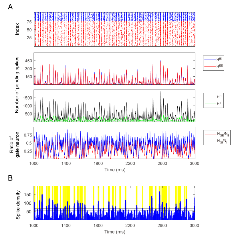
Figure 7: A 2s simulation of the full model in the Syn regime. A. Raster plot (top) and state space statistics (the other three panels). B. MFEs are recognized by the spiking volley detection algorithm.

Statistics

To quantify how well the reduced models (RN and CG) capture the dynamical features of the full model (MIF), we compare several statistics of the network dynamics (or more precisely, the spiking pattern produced by the network) collected from the simulations of the MIF, RN, and CG models. The reader should note that we can not tell the specific neuron indices of firing events in the CG model; yet it does not affect the computation of the statistics below. The raster plots produced for the CG model, however, are indeed mock-up raster plots, drawn by assigning spikes to neurons randomly among the appropriate $\{E,I\}$ population.

Firing rates. Spikes from $\{E,I\}$-cells are collected separately, and firing rates $(fr_{E},fr_{I})$ are computed as the average numbers of spikes per neuron per second. All three models are simulated simulated for over 3 seconds and spikes are collected from the 2nd second to rule out possible influences by the choice of initial conditions.

Spike synchrony index. We borrow the definition of spike synchrony index (SSI) from chariker2018rhythm (19). SSI describes the degree of synchrony of the firing events as the following. For each spike occurred at $t$, consider a $w$-ms time window centered by the spike $(t-\nicefrac{{w}}{{2}},t+\nicefrac{{w}}{{2}})$ and count the fraction of neurons in the whole network firing in such window. Finally, the SSI is the fraction averaged over all spikes.

It is not hard to see that SSI is larger for more synchronous spiking patterns. For the completely synchronized dynamics, every other neuron fires within the time window of each spike hence SSI=1. For completely uncorrelated firing patterns such as Poisson, SSI is a small number close to 0. One should note that the absolute value of SSI dependes on the choice of the window size, and we choose $w=5$ms (the same as chariker2018rhythm (19)).

Spectrogram. The power spectrum density (PSD) measures the variance in a signal as a function of frequency. In this study, the PSD is computed as follows:

A time interval $(0,T)$ is divide into time bins $B_{n}=[(n-1)\Delta t,n\Delta t],n=1,2,...$, the spike density $\mu_{n}$ per neuron in $B_{n}$ is given by $\mu_{n}=\nicefrac{{m_{n}}}{{N\Delta t}}$ where $m_{n}$ is the total number of spikes fired in bin $B_{n}$. Hence, the discrete Fourier transform of $\{\mu_{n}\}$ on $(0,T)$ is given as:

$$\hat{\mu}(k)=\frac{1}{\sqrt{T}}\sum_{n=1}^{\nicefrac{{T}}{{\Delta t}}}\mu_{n}\Delta te^{-k\cdot(2\pi i)\cdot(n\Delta t)}.$$ (13)

Finally, as a function of $k$, PSD is the “power” concentrated at frequency $k$, i.e., $|\hat{\mu}(k)|^{2}$.

Spike timing correlations. The correlation diagrams describe the averaged correlation between each spike and others. Consider the correlation with $I$-spikes conditioned on E at t = 0:

For each $E$-spike at time $t$, we take $I$-spikes within the time window $[t-15\mbox{ms},t+15\mbox{ms}]$, and compute the fraction of $I$-spikes in each 1-ms time bin. The correlation diagrams is then averaged over all $E$-spikes in this simulation.

Spiking volley detection. The method defining spiking volleys (or MFEs) is borrowed from chariker2015emergent (20). The core idea of this method is to find time intervals with some length constraints that the firing rate of each time bin in this interval is a certain amount higher than the average firing rate. This is then defined as a spiking volley. We choose 1 ms time bin and $\delta=0.33,\ \epsilon=8$ as parameters (Fig. 7B).

Computational Methods

Exact timing of events. During our simulation, we can compute the exact timing of all events including firing, kicks taking effect, etc. We note that MIF, RN, and CG models are all Markov processes whose randomness is mainly due to the exponential distributions of various waiting times. Consider two independent events $A$ and $B$ with waiting time $X_{A}\sim\mbox{exp}(\lambda_{A})$, $X_{B}\sim\mbox{exp}(\lambda_{B})$, we have $\min\{X_{A},X_{B}\}\sim\mbox{exp}(\lambda_{A}+\lambda_{B})$, i.e., the waiting time for either the first event is also an exponential distribution. Furthermore, the probability for the first occurring events to be $A$ is $\nicefrac{{\lambda_{A}}}{{(\lambda_{A}+\lambda_{B})}}$.

Similar arguments extend to $m$ events. By noticing that exponential distributed waiting times are temporally memoryless, we can simulated all three models by repeatedly selecting the first occurring event and generate the actual waiting time by sampling from certain exponential distributions.

Invariant probability distributions. After determining the total number of states and the transition probabilities between them, we can calculate the invariant probability distribution from the CG model by computing the eigenvectors and eigenvalues of the transition probability matrix. Such methods can be found in standard linear algebra textbooks such as roman2005advanced (61).

Readers should note that theoretically, there is no upper bound for $\{H^{E},H^{I}\}$. In order to close the computation of invariant probability distributions, we set the $n_{\{H^{E},H^{I}\}}$, the largest numbers of pending spikes shown up in the simulations as the “boundaries” of the state space. Specifically, the transition probability from state $X$ to $Y$ is 0 if

1. $X=(N_{GE},N_{GI},n_{H^{E}},H^{I})$ and $Y=(N_{GE},N_{GI},n_{H^{E}}+a,H^{I})$, or

2. $X=(N_{GE},N_{GI},H^{E},n_{H^{I}})$ and $Y=(N_{GE},N_{GI},H^{E},n_{H^{I}}+b)$,

where $a,b>0$.

A “Shrunk” Coarse Grained Model. After the reductions, the CG model studied in this paper still has $M=5.6\times 10^{9}$ states. Though the first left eigenvector (i.e., the stationary probability distribution, corresponding to eigenvalue 1) of a sparse, $M$-by-$M$ probability transition matrix is computable, the cost could be high for a desktop. Therefore, we aim at an even coarser version of the CG model: a “shrunk” coarse grained (SCG) model. Since $H^{\{E,I\}}$ are much higher than $N_{\{GE,GI\}}$, we shrink the CG model by combining every $K$ states of pending kicks into one, i.e., all $1\leq H^{E}_{\mbox{cg}}\leq K$ states in CG model is considered as $H^{E}_{\mbox{scg}}=1$ in SCG model. The intuition is the following: no need to characterize the states of pending spikes very precisely especially when the number is very large (i.e., the difference between 3000 and 3001 is very small). We choose $K=24$ to keep it the same as $S_{EE}$.

Every state of SCG model can also be represented as a quadruplet $\mathbb{Q}_{\mbox{scg}}=(N_{GE},N_{GI},H^{E}_{\mbox{scg}},H^{I}_{\mbox{scg}})$. The SCG model works as follow. Firstly the quadruple $\mathbb{Q}_{\mbox{scg}}$ is lifted to another quadruplet $\mathbb{Q}_{\mbox{cg}}=(N_{GE},N_{GI},H^{E}_{\mbox{cg}},H^{I}_{\mbox{cg}})$, where $H^{E,I}_{\mbox{cg}}=(H^{E,I}_{\mbox{scg}}-0.5)\cdot K$. Then quadruplet $\mathbb{Q}_{\mbox{cg}}$ acts following the same rule as the CG model. Lastly the change of $\mathbb{Q}_{\mbox{cg}}$ is projected back into the change of $\mathbb{Q}_{\mbox{scg}}$:

1. The change of $N_{GE}$ and $N_{GE}$ in $\mathbb{Q}_{\mbox{cg}}$ is kept the same on corresponding elements in $\mathbb{Q}_{\mbox{scg}}$;

2. The change $x$ of $H^{E,I}_{\mbox{cg}}$ is replaced by change $y=[x/K]+b$ on $H^{E,I}_{\mbox{scg}}$, where $[\cdot]$ denotes the least integer function and $b$ is a Bernoulli variable with probability $p=(x/K)-y$;

Through this model, we can further reduce the $M$ states of CG model to $M/K^{2}$ states of SCG model.

Locally-linear embedding. LLE is a nonlinear dimension reduction method which discovers the low-dimensional structure of high-dimensional data roweis2000nonlinear (62). More precisely, it maps the high-dimensional input data into a low-dimensional space. The core idea of LLE is to maintain the local linear structure through the mapping and this is achieved by a two-step optimization. There are $N$ input data and we denote the high-dimensional input as $\vec{X}_{i}$ and low-dimensional output as $\vec{Y}_{i}$. The algorithm is described below and more details see roweis2000nonlinear (62, 63).

1. Find the nearest $k$ neighbors $S_{i}^{k}$ of each data point $\vec{X}_{i}$;

2. $W=\mathop{\arg\min}_{W^{\prime}}\sum_{i}\|\vec{X}_{i}-\sum_{j}W_{ij}^{\prime}\vec{X}_{j}\|^{2}$,$\ W_{ij}^{\prime}=0$ if $\vec{X}_{j}\notin S_{i}^{k}$;

3. $Y=\mathop{\arg\min}_{Y^{\prime}}\sum_{i}\|\vec{Y}^{\prime}_{i}-\sum_{j}W_{ij}\vec{Y}^{\prime}_{j}\|^{2}$, subject to $\sum_{i}\vec{Y}^{\prime}_{i}=0$ and $\frac{1}{N}\sum_{i}\vec{Y}^{\prime}_{i}\vec{Y}_{i}^{\prime T}=I$;

Dimensionality of data. We use local principal component analysis (local PCA) method to compute the local dimensionality of the data at each data point $x$, i.e., how its neighbors cluster around $x$. The data points processed here is selected from original data points with probability proportional to the square of distance from the place with highest density mass, in order to make the distribution of data points more uniform which can result in more precise local dimensionality chracterization. For $x$, consider the correlation matrix $C_{x}$ of $x$ and its $K$ nearest neighbors ($K$ selected as 100). Then the dimensionality at $x$ is computed as

$$\mbox{Dim}(x)=\frac{\mbox{Tr}(C_{x})^{2}}{\mbox{Tr}(C_{x}^{2})}=\frac{(\sum_{i}\lambda_{i})^{2}}{\sum_{i}\lambda_{i}^{2}}$$ (14)

where $\lambda_{i}$ is the $i$-th eigenvalue of correlation matrix $C_{x}$. Eq. (14) is widely used as the dimensionality definition in theoretical and experimental neuroscience studies gao2017theory (31, 60, 49, 45).

Supplementary Materials

S1 Low-Dimension Manifolds

Trajectories of MIF and CG Models. Although MIF and CG models exhibit subtle difference in the statistics of the dynamics, we find that their trajectories in state space $(N_{GE},N_{GI},H^{E},H^{I})$ stay close to similar manifolds (Fig. S1).

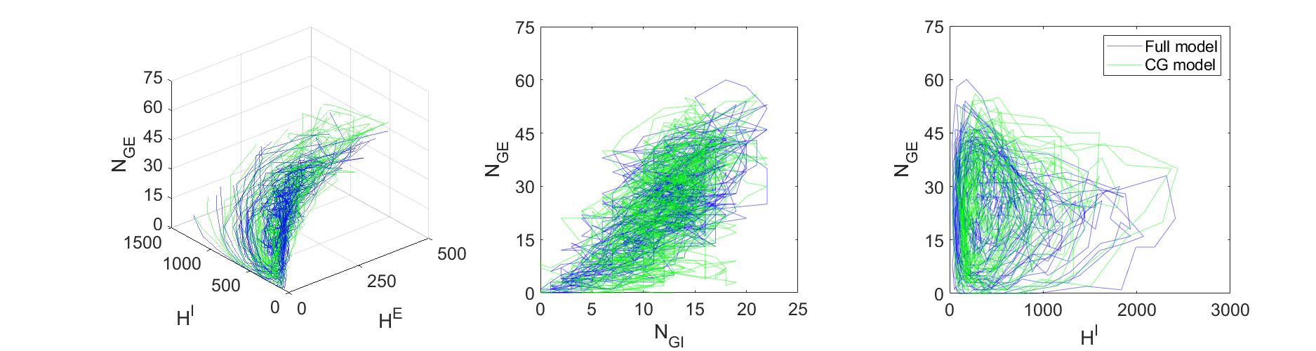
Figure S1: MIF and CG models produce trajectories on similar surfaces. Left: The projection on subspace $(N_{GE},H^{E},H^{I})$; Middle: The projection on subspace $(N_{GE},N_{GI})$; Right: The projection on subspace $(N_{GE},H^{I})$.

MIF Trajectories in Syn, Reg, and Hom Regimes. The low-dimensional manifolds in state spaces are powerful tools to visualize and analyze gamma dynamics. Here, we are interested in the comparison of manifolds for these three regimes studied in the manuscript. In the Syn regime, $X$ has a faster speed to consume the pending $E$-kicks (compared to Hom and Reg), i.e., $E$-neurons are faster recruited by the recurrent excitation, resulting in larger MFEs. These features are reflected by the full-model trajectories in the three different regimes (Fig. S2).

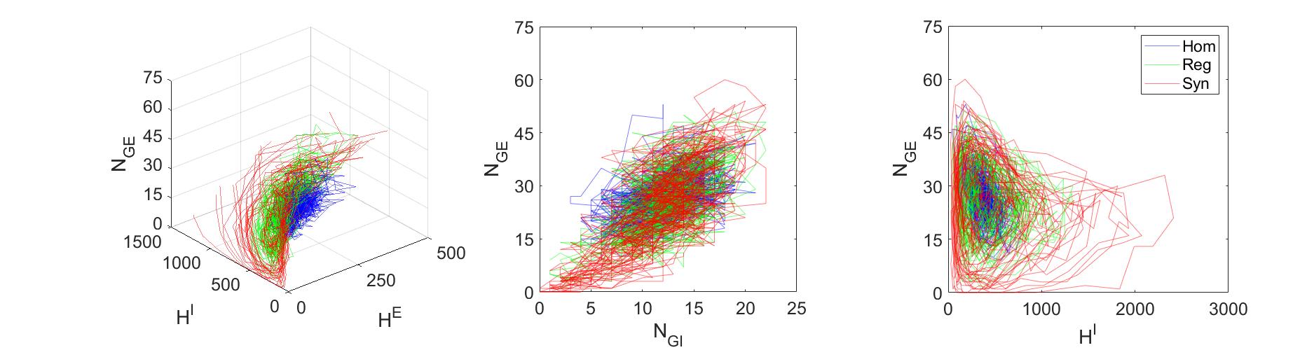
Figure S2: Full model trajectories of three regimes (Syn, Reg, and Hom). Left: The projection on subspace $(N_{GE},H^{E},H^{I})$; Middle: The projection on subspace $(N_{GE},N_{GI})$; Right: The projection on subspace $(N_{GE},H^{I})$.

S2 A Larger MIF Network

We repeat the model reduction for a 400-neuron MIF network, and collect the state space variables $(N_{GE},N_{GI},H^{E},H^{I})$ from a 100-second simulation (Fig. S3). A similar manifold is revealed by the trajectories in the state space, and also verified by the mass of trajectory density (Fig. S3AB). The two-dimensional local structure is also verified by the local dimensionality estimation and local linear embedding (Fig. S3CD). For this network, we simulate the Syn regime with parameters identical to li2019well (43).

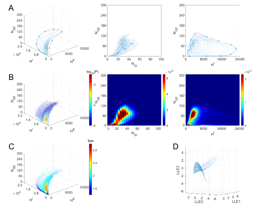
Figure S3: Gamma dynamics of a 400-neuron MIF network restricted on a low-dimensional manifold. A-D are similar to A, B, E, F of Fig. 6.

S3 Issues of Model Reduction

Selection of the cutoff. How faithful the RN models capture the full-model dynamics depends on the selection of cutoff $V^{c}$. Our assumption of RN is that the gamma dynamics is mostly sensitive to the subthreshold distribution of neurons about to fire. On the other hand, a high $V^{c}$ provides an accurate description of gate neurons, but very roughly for the base neurons, which is a potential issue for the RN model. For the RN model in this paper, we tuned the selection of the cutoff systematically and finally choose $V^{c}=40$. Here we present the firing rates and raster plots of the RN model when $V^{c}=70$ and $40$, where the former results in much larger firing rates and MFEs.

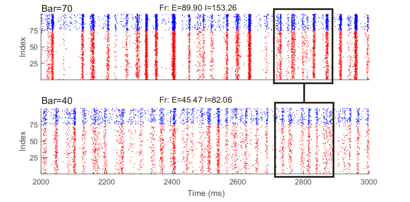
Figure S4: Raster plots of different cutoffs $V^{c}$ in the RN models. Upper: $V^{c}=70$; Lower: $V^{c}=40$.

The duration of MFEs. The MFEs of the reduced models have longer duration than the full model, possibly due to the slower probability flows since we combine multiple states from the full model as one in the reduced ones.

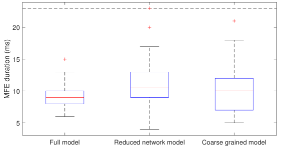
Figure S5: The duration of MFEs in different models. For each model, the mean (red line), first and third quartile (lower and upper bounds of the blue box), minimum and maximum (black lines), and outliers (red cross) are indicated in the box plot. The duration of MFEs for the RN and CG models are significantly higher than the full model (p = 0.004 and 0.038).

A 5-variable CG model. The 4-variable CG model combines $E$-kick pools of all neurons together, which may cause a problem since the pending $E$-kicks for $E$ neurons and $I$ neurons are consumed by different speeds. Hence we come up with a 5-variable version were $H_{EE}$ and $H_{IE}$ are counted separately.

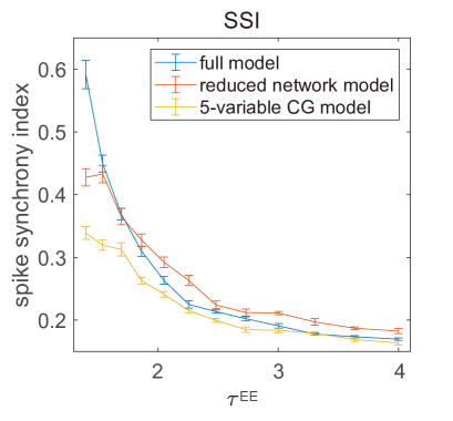
Figure S6: Degree of synchrony increases when $\tau^{EE}$ decreases. Reprinted from Fig. 5B, but the 4-variable CG model is replaced by a 5-variable version.

S4 Incorporate More Complicate Setup: NMDA Receptor and others

The model reduction introduced in this paper can be easily generalized for more complicated network setup. We present one example here.

In the main text, we only considered two synapse types (or more frankly, two synaptic time scales): AMPA and GABA, in this paper. To incorporate more types of synapse, such as NMDA ( 80 ms), we can introduce one more pending-kick pools $H^{\mbox{nmda}}_{i}$ for neuron $i$ in the MIF and RN models, and an additional pending-kick pool $H^{\mbox{nmda}}$ for the whole network. We note that this idea can be extended to multiple, heterogeneously coupled populations. In general, we may need to use states beyond base and gate, and the relevant pending-kick pools, as synaptic couplings become heterogeneous.

References

- (1) Peter Ashwin, Stephen Coombes and Rachel Nicks “Mathematical frameworks for oscillatory network dynamics in neuroscience” In The Journal of Mathematical Neuroscience 6.1 Springer, 2016, pp. 2
- (2) R. Azouz and C.M. Gray “Adaptive coincidence detection and dynamic gain control in visual cortical neurons in vivo” In Neuron 37, 2003, pp. 513–523
- (3) Rony Azouz and Charles M Gray “Dynamic spike threshold reveals a mechanism for synaptic coincidence detection in cortical neurons in vivo” In Proceedings of the National Academy of Sciences 97.14 National Acad Sciences, 2000, pp. 8110–8115
- (4) Erol Başar “A review of gamma oscillations in healthy subjects and in cognitive impairment” In International Journal of Psychophysiology 90.2, 2013, pp. 99–117 DOI: https://doi.org/10.1016/j.ijpsycho.2013.07.005
- (5) Elizabeth P Bauer, Rony Paz and Denis Paré “Gamma oscillations coordinate amygdalo-rhinal interactions during learning” In Journal of Neuroscience 27.35 Soc Neuroscience, 2007, pp. 9369–9379
- (6) Markus Bauer, Robert Oostenveld, Maarten Peeters and Pascal Fries “Tactile spatial attention enhances gamma-band activity in somatosensory cortex and reduces low-frequency activity in parieto-occipital areas” In Journal of Neuroscience 26.2 Soc Neuroscience, 2006, pp. 490–501
- (7) John M Beggs and Dietmar Plenz “Neuronal avalanches in neocortical circuits” In Journal of Neuroscience 23.35 Soc Neuroscience, 2003, pp. 11167–11177
- (8) Christian Bick, Marc Goodfellow, Carlo R Laing and Erik A Martens “Understanding the dynamics of biological and neural oscillator networks through exact mean-field reductions: a review” In The Journal of Mathematical Neuroscience 10.1 SpringerOpen, 2020, pp. 1–43
- (9) Christoph Börgers and Nancy Kopell “Synchronization in networks of excitatory and inhibitory neurons with sparse, random connectivity” In Neural Computation 15.3 MIT Press, 2003, pp. 509–538
- (10) Anatol Bragin et al. “Gamma (40-100 Hz) oscillation in the hippocampus of the behaving rat” In Journal of Neuroscience 15.1 Soc Neuroscience, 1995, pp. 47–60
- (11) Steven L Bressler “Context rules” In Behavioral and Brain Sciences 26.1 Cambridge University Press, 2003, pp. 85–85
- (12) Michael Brosch, Eike Budinger and Henning Scheich “Stimulus-related gamma oscillations in primate auditory cortex” In Journal of Neurophysiology 87.6 American Physiological Society Bethesda, MD, 2002, pp. 2715–2725
- (13) Nicolas Brunel and Vincent Hakim “Fast global oscillations in networks of integrate-and-fire neurons with low firing rates” In Neural Computation 11.7 MIT Press, 1999, pp. 1621–1671
- (14) Michael A Buice and Carson C Chow “Beyond mean field theory: statistical field theory for neural networks” In Journal of Statistical Mechanics: Theory and Experiment 2013.03 IOP Publishing, 2013, pp. P03003
- (15) T.J. Buschman and E.K. Miller “Top-down versus bottom-up control of attention in the prefrontal and posterior parietal cortices” In Science 315, 2007, pp. 1860–1862
- (16) György Buzsáki and Xiao-Jing Wang “Mechanisms of gamma oscillations” In Annual Review of Neuroscience 35 Annual Reviews, 2012, pp. 203–225
- (17) David Cai, Louis Tao, Aaditya V Rangan and David W McLaughlin “Kinetic theory for neuronal network dynamics” In Communications in Mathematical Sciences 4.1 International Press of Boston, 2006, pp. 97–127
- (18) Ryan T Canolty et al. “Oscillatory phase coupling coordinates anatomically dispersed functional cell assemblies” In Proceedings of the National Academy of Sciences 107.40 National Acad Sciences, 2010, pp. 17356–17361
- (19) Logan Chariker, Robert Shapley and Lai-Sang Young “Rhythm and synchrony in a cortical network model” In Journal of Neuroscience 38.40 Soc Neuroscience, 2018, pp. 8621–8634
- (20) Logan Chariker and Lai-Sang Young “Emergent spike patterns in neuronal populations” In Journal of Computational Neuroscience 38.1 Springer, 2015, pp. 203–220
- (21) Mark M Churchland et al. “Stimulus onset quenches neural variability: a widespread cortical phenomenon” In Nature Neuroscience 13.3 Nature Publishing Group, 2010, pp. 369–378
- (22) L. Colgin et al. “Frequency of gamma oscillations routes flow of information in the hippocampus” In Nature 462, 2009, pp. 75–78
- (23) Laura Lee Colgin “Rhythms of the hippocampal network” In Nature Reviews Neuroscience 17.4 Nature Publishing Group, 2016, pp. 239–249
- (24) Jack D Cowan “Stochastic neurodynamics” In Advances in Neural Information Processing Systems, 1991, pp. 62–69
- (25) J. Csicsvari, B. Jamieson, K. Wise and G. Buzsáki “Mechanisms of gamma oscillations in the hippocampus of the behaving rat” In Neuron 37, 2003, pp. 311–322
- (26) M. Diesmann, M.. Gewaltig and A. Aertsen “Stable propagation of synchronous spiking in cortical neural networks” In Nature 402, 1999, pp. 529–533
- (27) Axel Frien et al. “Fast oscillations display sharper orientation tuning than slower components of the same recordings in striate cortex of the awake monkey” In European Journal of Neuroscience 12.4 Wiley Online Library, 2000, pp. 1453–1465
- (28) P. Fries, J.H. Reynolds, A.E. Rorie and R. Desimone “Modulation of oscillatory neuronal synchronization by selective visual attention” In Science 291, 2001, pp. 1560–1563
- (29) Pascal Fries “Neuronal gamma-band synchronization as a fundamental process in cortical computation” In Annual Review of Neuroscience 32 Annual Reviews, 2009, pp. 209–224
- (30) Pascal Fries, Thilo Womelsdorf, Robert Oostenveld and Robert Desimone “The effects of visual stimulation and selective visual attention on rhythmic neuronal synchronization in macaque area V4” In Journal of Neuroscience 28.18 Soc Neuroscience, 2008, pp. 4823–4835
- (31) Peiran Gao et al. “A theory of multineuronal dimensionality, dynamics and measurement” In BioRxiv Cold Spring Harbor Laboratory, 2017, pp. 214262
- (32) Wulfram Gerstner, Werner M Kistler, Richard Naud and Liam Paninski “Neuronal Dynamics: From Single Neurons to Networks and Models of Cognition” Cambridge University Press, 2014
- (33) C Alex Goddard, Devarajan Sridharan, John R Huguenard and Eric I Knudsen “Gamma oscillations are generated locally in an attention-related midbrain network” In Neuron 73.3 Elsevier, 2012, pp. 567–580
- (34) C.M. Gray, P. König, A.K. Engel and W. Singer “Oscillatory responses in cat visual cortex exhibit inter-columnar synchronization which reflects global stimulus properties” In Nature 338, 1989, pp. 334–337
- (35) G.G. Gregoriou, S.J. Gotts, H. Zhou and R. Desimone “High-frequency, long-range coupling between prefrontal and visual cortex during attention” In Science 324, 2009, pp. 1207–1210
- (36) J Andrew Henrie and Robert Shapley “LFP power spectra in V1 cortex: the graded effect of stimulus contrast” In Journal of Neurophysiology 94.1 American Physiological Society, 2005, pp. 479–490
- (37) Alan L Hodgkin and Andrew F Huxley “A quantitative description of membrane current and its application to conduction and excitation in nerve” In The Journal of Physiology 117.4 Wiley-Blackwell, 1952, pp. 500
- (38) Yu Hu, James Trousdale, Krešimir Josić and Eric Shea-Brown “Motif statistics and spike correlations in neuronal networks” In Journal of Statistical Mechanics: Theory and Experiment 2013.03 IOP Publishing, 2013, pp. P03012
- (39) Stephen Keeley, Áine Byrne, André Fenton and John Rinzel “Firing rate models for gamma oscillations” In Journal of Neurophysiology 121.6 American Physiological Society Bethesda, MD, 2019, pp. 2181–2190
- (40) John H Krystal et al. “Impaired tuning of neural ensembles and the pathophysiology of schizophrenia: a translational and computational neuroscience perspective” In Biological Psychiatry 81.10 Elsevier, 2017, pp. 874–885
- (41) C.. Laing “The dynamics of networks of identical theta neurons” In Journal of Mathematical Neuroscience 8.1, 2018, pp. 4
- (42) Kwang-Hyuk Lee, Leanne M Williams, Michael Breakspear and Evian Gordon “Synchronous gamma activity: a review and contribution to an integrative neuroscience model of schizophrenia” In Brain Research Reviews 41.1 Elsevier, 2003, pp. 57–78
- (43) Yao Li, Logan Chariker and Lai-Sang Young “How well do reduced models capture the dynamics in models of interacting neurons?” In Journal of Mathematical Biology 78.1-2 Springer, 2019, pp. 83–115
- (44) Yao Li and Hui Xu “Stochastic neural field model: multiple firing events and correlations” In Journal of Mathematical Biology 79.4 Springer, 2019, pp. 1169–1204
- (45) Ashok Litwin-Kumar et al. “Optimal degrees of synaptic connectivity” In Neuron 93.5 Elsevier, 2017, pp. 1153–1164
- (46) Jing Liu and William T Newsome “Local field potential in cortical area MT: stimulus tuning and behavioral correlations” In Journal of Neuroscience 26.30 Soc Neuroscience, 2006, pp. 7779–7790
- (47) N.. Logothetis et al. “Neurophysiological investigation of the basis of the fMRI signal” In Nature 412.6843, 2001, pp. 150–157
- (48) Alexandra J Mably and Laura Lee Colgin “Gamma oscillations in cognitive disorders” In Current Opinion in Neurobiology 52 Elsevier, 2018, pp. 182–187
- (49) Luca Mazzucato, Alfredo Fontanini and Giancarlo La Camera “Stimuli reduce the dimensionality of cortical activity” In Frontiers in Systems Neuroscience 10 Frontiers, 2016, pp. 11
- (50) James M McNally and Robert W McCarley “Gamma band oscillations: a key to understanding schizophrenia symptoms and neural circuit abnormalities” In Current Opinion in Psychiatry 29.3 NIH Public Access, 2016, pp. 202
- (51) W Pieter Medendorp et al. “Oscillatory activity in human parietal and occipital cortex shows hemispheric lateralization and memory effects in a delayed double-step saccade task” In Cerebral Cortex 17.10 Oxford University Press, 2007, pp. 2364–2374
- (52) V Menon et al. “Spatio-temporal correlations in human gamma band electrocorticograms” In Electroencephalography and Clinical Neurophysiology 98.2 Elsevier, 1996, pp. 89–102
- (53) Ernest Montbrió, Diego Pazó and Alex Roxin “Macroscopic description for networks of spiking neurons” In Physical Review X 5.2 APS, 2015, pp. 021028
- (54) Bijan Pesaran et al. “Temporal structure in neuronal activity during working memory in macaque parietal cortex” In Nature Neuroscience 5.8 Nature Publishing Group, 2002, pp. 805–811
- (55) Dietmar Plenz et al. “Multi-electrode array recordings of neuronal avalanches in organotypic cultures” In JoVE (Journal of Visualized Experiments), 2011, pp. e2949
- (56) Andrei T Popescu, Daniela Popa and Denis Paré “Coherent gamma oscillations couple the amygdala and striatum during learning” In Nature Neuroscience 12.6 Nature Publishing Group, 2009, pp. 801–807
- (57) A.. Rangan and L.. Young “Dynamics of spiking neurons: between homogeneity and synchrony” In Journal of Computational Neuroscience 34.3, 2013, pp. 433–460
- (58) A.. Rangan and L.. Young “Emergent dynamics in a model of visual cortex” In Journal of Computational Neuroscience 35.2, 2013, pp. 155–167
- (59) Supratim Ray and John HR Maunsell “Do gamma oscillations play a role in cerebral cortex?” In Trends in Cognitive Sciences 19.2 Elsevier, 2015, pp. 78–85
- (60) Stefano Recanatesi, Gabriel Koch Ocker, Michael A Buice and Eric Shea-Brown “Dimensionality in recurrent spiking networks: global trends in activity and local origins in connectivity” In PLoS Computational Biology 15.7 Public Library of Science, 2019, pp. e1006446
- (61) Steven Roman, S Axler and FW Gehring “Advanced Linear Algebra” Springer, 2005
- (62) Sam T Roweis and Lawrence K Saul “Nonlinear dimensionality reduction by locally linear embedding” In Science 290.5500 American Association for the Advancement of Science, 2000, pp. 2323–2326
- (63) Lawrence K Saul and Sam T Roweis “An introduction to locally linear embedding” In unpublished. Available at: http://www. cs. toronto. edu/~ roweis/lle/publications. html, 2000
- (64) Woodrow L Shew et al. “Information capacity and transmission are maximized in balanced cortical networks with neuronal avalanches” In Journal of Neuroscience 31.1 Soc Neuroscience, 2011, pp. 55–63
- (65) Markus Siegel, Tobias H Donner and Andreas K Engel “Spectral fingerprints of large-scale neuronal interactions” In Nature Reviews Neuroscience 13.2 Nature Publishing Group, 2012, pp. 121–134
- (66) Markus Siegel, Melissa R Warden and Earl K Miller “Phase-dependent neuronal coding of objects in short-term memory” In Proceedings of the National Academy of Sciences 106.50 National Acad Sciences, 2009, pp. 21341–21346
- (67) T. Sigurdsson et al. “Impaired hippocampal-prefrontal synchrony in a genetic mouse model of schizophrenia” In Nature 464, 2010, pp. 763–767
- (68) V.S. Sohal, F. Zhang, O. Yizhar and K. Deisseroth “Parvalbumin neurons and gamma rhythms enhance cortical circuit performance” In Nature 459, 2009, pp. 698–702
- (69) Sen Song et al. “Highly nonrandom features of synaptic connectivity in local cortical circuits” In PLoS Biology 3.3 Public Library of Science, 2005, pp. e68
- (70) Catherine Tallon-Baudry “The roles of gamma-band oscillatory synchrony in human visual cognition” In Frontiers in Bioscience (Landmark Ed) 14, 2009, pp. 321–332
- (71) Jianjun Paul Tian and D Kannan “Lumpability and commutativity of Markov processes” In Stochastic Analysis and Applications 24.3 Taylor & Francis, 2006, pp. 685–702
- (72) Roger D Traub et al. “Single-column thalamocortical network model exhibiting gamma oscillations, sleep spindles, and epileptogenic bursts” In Journal of Neurophysiology 93.4 American Physiological Society, 2005, pp. 2194–2232
- (73) Matthijs AA Van Der Meer and A David Redish “Low and high gamma oscillations in rat ventral striatum have distinct relationships to behavior, reward, and spiking activity on a learned spatial decision task” In Frontiers in Integrative Neuroscience 3 Frontiers, 2009, pp. 9
- (74) Marijn Wingerden, Martin Vinck, Jan V Lankelma and Cyriel MA Pennartz “Learning-associated gamma-band phase-locking of action–outcome selective neurons in orbitofrontal cortex” In Journal of Neuroscience 30.30 Soc Neuroscience, 2010, pp. 10025–10038
- (75) Xiao-Jing Wang “Neurophysiological and computational principles of cortical rhythms in cognition” In Physiological Reviews 90.3 American Physiological Society Bethesda, MD, 2010, pp. 1195–1268
- (76) Xiao-Jing Wang and György Buzsáki “Gamma oscillation by synaptic inhibition in a hippocampal interneuronal network model” In Journal of Neuroscience 16.20 Soc Neuroscience, 1996, pp. 6402–6413
- (77) Zhuo Wang, Andrew T Sornborger and Louis Tao “Graded, dynamically routable information processing with synfire-gated synfire chains” In PLoS Computational Biology 12.6 Public Library of Science San Francisco, CA USA, 2016, pp. e1004979
- (78) Miles A Whittington et al. “Inhibition-based rhythms: experimental and mathematical observations on network dynamics” In International Journal of Psychophysiology 38.3 Elsevier, 2000, pp. 315–336
- (79) Hugh R Wilson and Jack D Cowan “Excitatory and inhibitory interactions in localized populations of model neurons” In Biophysical Journal 12.1 Elsevier, 1972, pp. 1–24
- (80) Hugh R Wilson and Jack D Cowan “A mathematical theory of the functional dynamics of cortical and thalamic nervous tissue” In Kybernetik 13.2 Springer, 1973, pp. 55–80
- (81) T. Womelsdorf et al. “Modulation of neuronal interactions through neuronal synchronization” In Science 316, 2007, pp. 1609–1612
- (82) Thilo Womelsdorf et al. “Orientation selectivity and noise correlation in awake monkey area V1 are modulated by the gamma cycle” In Proceedings of the National Academy of Sciences 109.11 National Acad Sciences, 2012, pp. 4302–4307
- (83) Zhuocheng Xiao, Jiwei Zhang, Andrew T Sornborger and Louis Tao “Cusps enable line attractors for neural computation” In Physical Review E 96.5 APS, 2017, pp. 052308
- (84) Dajun Xing et al. “Stochastic generation of gamma-band activity in primary visual cortex of awake and anesthetized monkeys” In Journal of Neuroscience 32.40 Soc Neuroscience, 2012, pp. 13873–13880a
- (85) Jianing Yu and David Ferster “Membrane potential synchrony in primary visual cortex during sensory stimulation” In Neuron 68.6 Elsevier, 2010, pp. 1187–1201
- (86) Shan Yu et al. “Higher-order interactions characterized in cortical activity” In Journal of Neuroscience 31.48 Soc Neuroscience, 2011, pp. 17514–17526
- (87) J. Zhang, K. Newhall, D. Zhou and A. Rangan “Distribution of correlated spiking events in a population-based approach for Integrate-and-Fire networks” In Journal of Computational Neuroscience 36.2, 2014, pp. 279–295
- (88) J. Zhang, D. Zhou, D. Cai and A.. Rangan “A coarse-grained framework for spiking neuronal networks: between homogeneity and synchrony” In Journal of Computational Neuroscience 37.1, 2014, pp. 81–104
- (89) J.. Zhang and A.. Rangan “A reduction for spiking integrate-and-fire network dynamics ranging from homogeneity to synchrony” In Journal of Computational Neuroscience 38.2, 2015, pp. 355–404
- (90) Liqiong Zhao, Bryce II Beverlin, Tay Netoff and Duane Quinn Nykamp “Synchronization from second order network connectivity statistics” In Frontiers in Computational Neuroscience 5 Frontiers, 2011, pp. 28