Characterizing Intersectional Group Fairness with Worst-Case Comparisons

Abstract

Machine Learning or Artificial Intelligence algorithms have gained considerable scrutiny in recent times owing to their propensity towards imitating and amplifying existing prejudices in society. This has led to a niche but growing body of work that identifies and attempts to fix these biases. A first step towards making these algorithms more fair is designing metrics that measure unfairness. Most existing work in this field deals with either a binary view of fairness (protected vs. unprotected groups) or politically defined categories (race or gender). Such categorization misses the important nuance of intersectionality - biases can often be amplified in subgroups that combine membership from different categories, especially if such a subgroup is particularly underrepresented in historical platforms of opportunity.

In this paper, we discuss why fairness metrics need to be looked at under the lens of intersectionality, identify existing work in intersectional fairness, suggest a simple worst case comparison method to expand the definitions of existing group fairness metrics to incorporate intersectionality, and finally conclude with the social, legal and political framework to handle intersectional fairness in the modern context.

1 Introduction

The use of machine learning algorithms is ubiquitous in the developed world. It has become an integral part of society, affecting the lives of millions of people. Algorithmic decisions vary from low-stakes determinations, like product or film recommendations, to high-impact like loan or credit approval Mukerjee et al. (2002), hiring recommendations Bogen and Rieke (2018), facial recognition Vasilescu and Terzopoulos (2002) and prison recidivism Corbett-Davies and Goel (2018). With this direct impact on people’s lives, the need for fair and unbiased algorithms is paramount. It is critical that algorithms do not replicate and enhance existing societal biases, including those rooted in differences of race, gender, or sexual orientation.

To tackle these problems, both fairness and bias need to be clearly defined. Currently, there does not exist a single universally agreed upon definition of fairness. Anti-discrimination legislation exists in various jurisdictions around the world. In the US, anti-discrimination laws exist under the Civil Rights Act Berg (1964), and under specific areas like credit lending and housing. There have also been efforts to introduce legislation combating algorithmic bias. In the European Union, the General Data Protection Regulation (GDPR) provides for regulations regarding digital profiling, data collection, and a right to explanation Goodman and Flaxman (2017). Under Indian law, quotas for scheduled castes, scheduled tribes and other backward classes are mandated in public education and government employment.

We begin with the broad definition of fairness as the absence of prejudice or preference for an individual or group based on their characteristics. Bias can also exist in a variety of forms. Mehrabi et al. (2019) provides an excellent overview on the differing types of bias and discrimination. In general, a fair machine learning algorithm is one that does not favor or make prejudice towards an individual or a group.

While most early fairness research focused on binary fairness metrics (protected vs. unprotected groups), newer methods to address fairness have begun to incorporate intersectional frameworks. These frameworks are derived from the third wave of feminist thought, which is rooted in the understanding of the interconnected nature of social categories, like race, gender, sexual orientation, and class Crenshaw (1989). The intersection of these categories creates differing levels of privilege or disadvantage for the various possible subgroups. There exist legal precedents for discrimination under an intersectional lens : The Equal Employment Opportunity Commission (EEOC) describes some Intersectional Discrimination/Harassment examples. Buolamwini and Gebru (2018) examined gender classification algorithms for facial image data and found that they performed substantially better on male faces than female faces. However, the largest performance drops came when both race and gender were considered, with darker skinned women disproportionately affected having a misclassification rate of $\approx$30%.

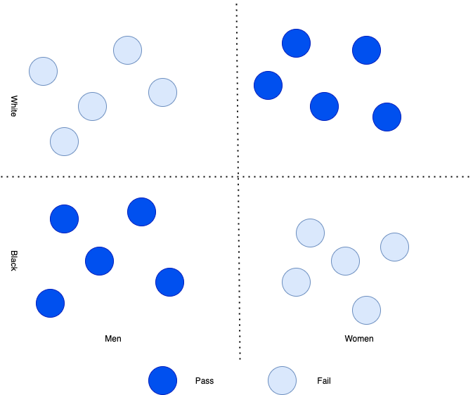
Figure 1: An example of “fairness gerrymandering”

The example in Figure 1 describes the importance of intersectional fairness. In the figure, we observe equal numbers of black and white people pass. Similarly, there is an equal number of men and women passing. However, this classification is unfair because we don’t have any black women and white men that passed, and all black men and white women passed. We observe the bias only while looking at the subgroups when we take race and gender as protected attributes. This phenomenon was called Fairness Gerrymandering by Kearns et al. (2018).

Additionally, there are minorities that have historically faced discrimination around the world, but due to their sparse population, empirical evidence of discrimination against them is difficult to trace, for example, the indigenous population Paradies (2006); King et al. (2009), or trans people Feldman et al. (2016); Reisner et al. (2016); Bockting et al. (2016). This causes machine learning practitioners to either disinclude these groups from their training datasets due to statistical insignificance, or worse, conflate them with other minorities to create a general protected category, which leads to the same sort of neglected bias as shown in figure 1.

In this paper, we discuss the notion of intersectional group fairness. After introducing existing related work, we define a combinatorial approach giving subsets of the population. With this definition of subgroups, we introduce a measure of the worst case disparity using existing fairness metrics, to discover biases against underserved subgroups. We then show how this method can be applied to classification models, ranking models, and models with continuous output. We end the paper with a discussion about the limitations of our approach and future work.

2 Related Work

2.1 Individual and Group Fairness

Fair machine learning differentiates group and individual fairness measures. While group fairness metrics focus on treating two different groups equally, individual fairness metrics focus on treating similar individuals similarly. Binns (2019) introduces those two notions and discusses the motivations behind individual and group fairness. In this paper, we focus on group fairness metrics.

2.2 Binary fairness metrics

A large majority of research in algorithmic fairness has covered fairness metrics for a single protected attribute Corbett-Davies and Goel (2018). Hardt et al. (2016) introduces the definitions of Equalized odds and equal opportunity, two measures for discrimination against a binary sensitive attribute. Verma and Rubin (2018) collected some known binary fairness metrics for classification models and demonstrated each metric with a unique example on the German credit dataset. In their example, the protected class is Gender, which has two values female and male.

2.3 Intersectional Fairness

More recently, however, some work has begun to address the issue of intersectionality in AI by providing statistical frameworks that control for bias within multiple subgroups. Hébert-Johnson et al. (2018) introduces the idea of multi-calibration which gives meaningful predictions for overlapping subgroups in a larger protected group. Kearns et al. (2018) developed an analogous method named rich subgroup fairness for false positive and negative constraints that hold over an infinitely large collection of subgroups. Kim et al. (2019) extend these methods for classifiers to be equally accurate on a combinatorially large collection of all subgroups. Mary et al. (2019) present the Renyi correlation coefficient as a fairness metric for datasets with continuous protected attributes. Finally, Foulds et al. (2020) introduce differential fairness (DF), as an intersectional fairness metric.

3 Intersectional group fairness metrics

In this section, we discuss our intersectional fairness metrics framework. We outline our definition of a subgroup of the population, define a worst case disparity metric that we call the min-max ratio and describe how we can operationalize the notion of min-max ratio to encompass intersectionality in existing metrics of fairness.

3.1 Subgroup definition

For the purposes of this paper, similar to Kearns et al. (2018), we define a subgroup $sg_{a_{1}....a_{n}}$ as a set containing the intersection of all members who belong to groups $g_{a_{1}}$ through $g_{a_{n}}$, where $a_{1}$, $a_{2}$…$a_{n}$ are marginal protected attributes, like race, gender, etc. Formally,

$$sg_{a_{1}\times a_{2}\times...\times a_{n}}=g_{a_{1}}\cap g_{a_{2}}...\cap g_{a_{n}}$$ (1)

Hence, for example, if $g_{1}$(race) $\in$ {black, white} and $g_{2}$(gender) $\in$ {man, woman}, then $sg\in$ {black women, black men, white women, white men} and N = $|sg|=2\times 2=4$.

This combinatorial, or cartesian product of attributes approach gives us subsets of the original dataset, where in each subgroup, the members have all the protected attributes of the groups they were composed of.

3.2 Worst Case Disparity

We introduce a simple concept to measure the worst case disparity using existing fairness metrics to incorporate intersectionality - the min-max ratio. In the vein of Rawls (2001) principle for distributive justice, the idea essentially is to measure the value of the given fairness metric for every subgroup $sg_{i}$ then take the ratio of the minimum and maximum values from this given list. The further this ratio is from 1, the greater the disparity is between subgroups. This min-max ratio technique allows us to encompass the entire breadth of possible subgroups in a dataset, by considering the worst case scenario in terms of adverse impact. For fairness metrics that are already comparative ratios of two groups, we redefine it by calculating the said ratio for all possible permutations of two subgroups and then simply take the minimum, also the worst possible case.

We discuss some of the most commonly used metrics in the literature below and show how we use the worst possible case framing to incorporate intersectionality.

3.3 Fair Classification metrics

Several fair classification metrics exist in literature. We discuss four group fairness metrics below from Mehrabi et al. (2019) and Gartner (2020).

3.3.1 Demographic parity

According to demographic parity, the proportion of each segment of a protected class should receive positive outcomes at equal rates. Mathematically, demographic parity compares the pass rate (rate of positive outcome) of two groups. Demographic parity is satisfied for a predictor $\hat{Y}$ and for a member $A$ if:

$$P(\hat{Y}|A\in sg_{i})=P(\hat{Y}|A\in sg_{j});\forall i,j\in N,i\neq j$$ (2)

where N is the total number of subgroups. Demographic parity is also known as statistical parity Dwork et al. (2012); Kusner et al. (2017).

Using our worst case, min-max ratio definition, Demographic parity ratio (DPR) would be defined as:

$$\text{DPR}=\frac{\text{min}\{P(\hat{Y}|A\in sg_{i})\forall i\in N\}}{\text{max}\{P(\hat{Y}|A\in sg_{i})\forall i\in N\}}$$ (3)

Disparate impact, as defined under the guideline by the Equal Employment Opportunity Commission et al. (1979) is similar to the demographic parity metric. It is intended as a way to measure indirect and unintentional discrimination in which certain decisions disproportionately affect members of a protected group. Disparate impact compares the pass rate of one group versus another. The Four-Fifths rule states that the ratio of the pass rate of group 1 to the pass rate of group 2 has to be greater than 80% (groups 1 and 2 interchangeable). Using our worst case definition, intersectional disparate impact (DI) is defined as the minimum disparate impact between all possible pairs of subgroups $sg$.

$$\text{DI}=\text{min}\left\{\frac{P(\hat{Y}|A\in sg_{i})}{P(\hat{Y}|A\in sg_{j})};\forall i,j\in N,i\neq j\right\}$$ (4)

3.3.2 Conditional statistical parity

Conditional statistical parity extends demographic parity by permitting a set of legitimate attributes to affect the outcome Corbett-Davies et al. (2017). Conditional statistical parity is satisfied for a predictor $\hat{Y}$, a member $A$ with a set of legitimate attributes $L$ if:

$$P(\hat{Y}|L=1,A\in sg_{i})=P(\hat{Y}|L=1,A\in sg_{j})\forall i,j\in N,i\neq j$$ (5)

Using the worst case, min-max ratio definition, Conditional statistical parity ratio (CSPR) would be defined just like equation 3:

$$\text{CSPR}=\frac{\text{min}\{P(\hat{Y}|L=1,A\in sg_{i})\forall i\in N\}}{\text{max}\{P(\hat{Y}|L=1,A\in sg_{i})\forall i\in N\}}$$ (6)

3.3.3 Equal opportunity

Equal opportunity or True Positive Rate Parity states that all members should be treated equally or similarly and not disadvantaged by prejudice or bias. Mathematically, it compares True Positive Rate (TPR) of the classifier between the protected group and the unprotected group Hardt et al. (2016). Equal opportunity for a binary predictor $\hat{Y}$ and a member $A$, is satisfied if:

$$P(\hat{Y}=1|A\in sg_{i},Y=1)=P(\hat{Y}=1|A\in sg_{j},Y=1)\forall i,j\in N,i\neq j$$ (7)

Using the worst case, min-max ratio definition, Equal opportunity ratio (EOppR) would be defined as:

$$\text{EOppR}=\frac{\text{min}\{P(\hat{Y}=1|A\in sg_{i},Y=1)\forall i\in N\}}{\text{max}\{P(\hat{Y}=1|A\in sg_{i},Y=1)\forall i\in N\}}$$ (8)

In a similar vein, there can exist True Negative Rate Parity, False Positive Rate Parity and False Negative Rate Parity. Hardt et al. (2016) propose Equalized Odds as a method to generalize the Equal Opportunity metric by comparing all these different parities.

3.3.4 Group Benefit Equality

Group Benefit Equality, introduced by Gartner (2020) aims to be useful in the domain of healthcare. Group benefit equality measures the predicted rate of passing for a subgroup compared to the actual rate of passing. Mathematically, this is defined as:

$$\begin{split}P(\hat{Y}|A\in sg_{i})=P(Y|A\in sg_{i})\forall i\in N\end{split}$$ (9)

And, Group benefit ratio for a subgroup is defined as:

$$\text{GBR}_{sg_{i}}=\frac{P(\hat{Y}|A\in sg_{i})}{P(Y|A\in sg_{i})};\forall i\in N$$ (10)

Using the worst case, min-max ratio definition, Group benefit ratio (GBR_INT) would be defined intersectionally as:

$$\text{GBR\_INT}=\frac{\text{min}\{\text{GBR}_{sg_{i}},\forall i\in N\}}{\text{max}\{\text{GBR}_{sg_{i}},\forall i\in N\}}$$ (11)

3.4 Multi-class classification models

For multiclass classification models, we present a modified version of the Equalized Odds metric, except instead of a binary positive or negative label, we measure the odds ratio for each possible discrete output, and then take the worst odds ratio among all outputs.

For instance, if a multiclass classifier has five possible output classes, we calculate the min-max ratio for each output class $y$, and then take the minimum of those five values as our final metric, since it is the worst possible scenario. Formally, Multiclass Equalized Odds Ratio (M-EOddR) is defined as:

$$\text{M-EOddR}=\text{min}\left\{\frac{\text{min}\{P(\hat{Y}=y_{k}|A\in sg_{i}),\forall i\in N\}}{\text{max}\{P(\hat{Y}=y_{k}|A\in sg_{i}),\forall i\in N\}}\right\}\forall k\in K$$ (12)

where K is the set of all possible output classes. The closer the value of M-EOddR is to 1, the lower the disparity is of the classifier’s performance among the various subgroups for all possible output classes.

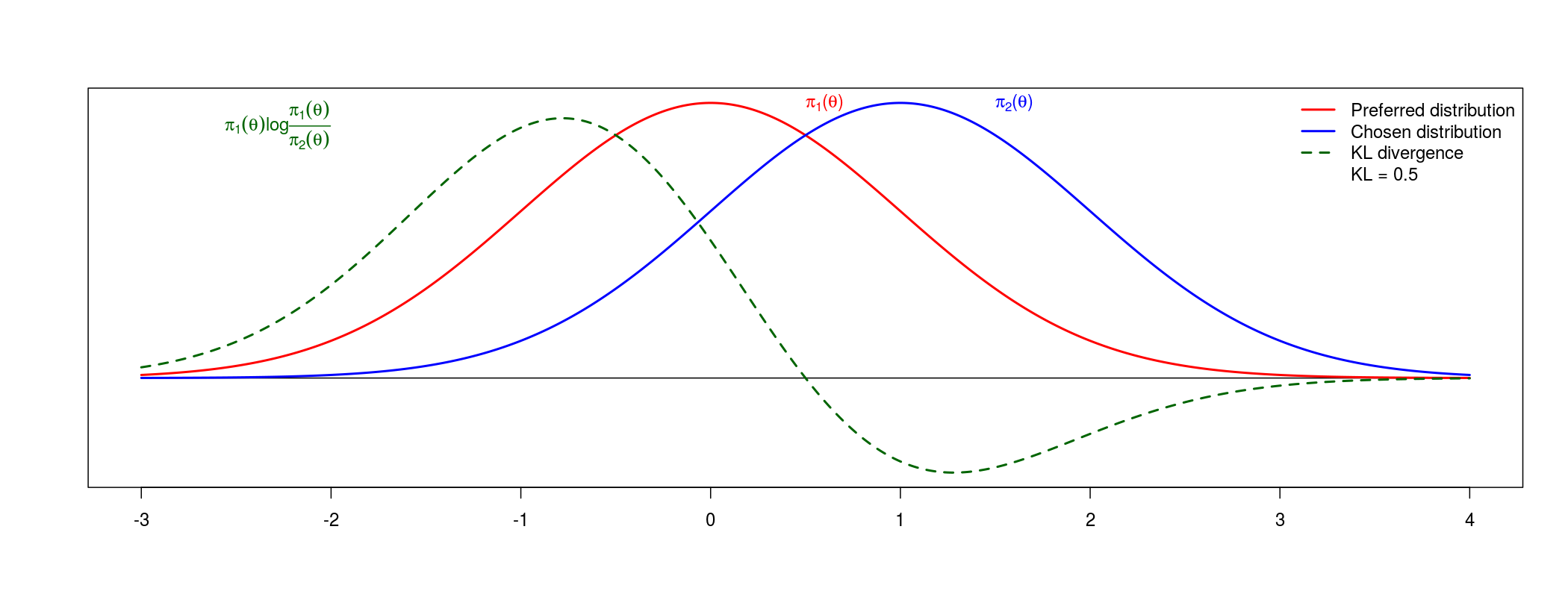
Figure 2: KL divergence example between two distributions adapted from Veen et al. (2018). In this example $\pi_{1}$ is a standard normal distribution and $\pi_{2}$ is a normal distribution with a mean of 1 and a variance of 1. The value of the KL divergence is equal to the area under the curve of the function (green line). The area under the green line above the x-axis adds to the divergence, while the area under the x-axis subtracts from the divergence.

3.5 Models with continuous output

We can extend the worst possible case framing for models which produce a continuous output, like regression models, or recommendation models that provide relevance scores. The Kullback-Leibler (KL) divergence between two distributions $q$ and $p$ is defined as the following:

$$D_{KL}(\pi_{1}||\pi_{2})=\int_{\infty}^{\infty}\pi_{1}(x)log(\frac{\pi_{1}(x)}{\pi_{2}(x)})dx$$ (13)

In the context of intersectional fairness, we compute the KL divergence between the model output distributions of all possible pairs of two subgroups, and we display the maximum KL divergence value obtained, since it is the worst case scenario. If this value is close to 0, the two subgroups have similar distributions, as well as the other subgroups.

Thus, Worst case KL Divergence (W-$D_{KL}$) is formally defined as:

$$\text{W-}D_{KL}=\text{max}\left\{\int_{\infty}^{\infty}\pi_{sg_{i}}(x)log(\frac{\pi_{sg_{i}}(x)}{\pi_{sg_{j}}(x)}\,dx\right\}\forall i,j\in N,i\neq j$$ (14)

3.6 Ranking metrics

Existing fair ranking metrics in the literature can be divided broadly into two classes - representation based Yang and Stoyanovich (2017) and exposure based Singh and Joachims (2018); Sapiezynski et al. (2019). We pick one of each kind and redefine them under the light of intersectionality.

3.6.1 Skew

The representation-based metric we discuss is skew@k Geyik et al. (2019). For a ranked list $\tau$, the Skew for subgroup $sg_{i}$ at the top $k$ is defined as

$$\text{Skew}_{sg_{i}}@k(\tau)=\frac{p_{\tau^{k},sg_{i}}}{p_{q,sg_{i}}}$$ (15)

where $p_{\tau^{k},sg_{i}}$ represents the fraction of members from subgroup $sg_{i}$ among the top $k$ items in $\tau$, and $p_{q,g_{i}}$ represents the fraction of members from to subgroup $sg_{i}$ in the overall population $q$. Ideally, $\text{Skew}_{g_{i}}@k$ should be close to one for each $sg_{i}$ and $k$, to show that people from $sg_{i}$ are represented in $\tau$ proportionally relative to the overall population.

Using our worst case method, the skew ratio at K (SR@K) is defined as:

$$\text{SR@K}=\frac{\text{min}\{\text{Skew}_{sg_{i}}@k(\tau),\forall i\in N\}}{\text{max}\{\text{Skew}_{sg_{i}}@k(\tau),\forall i\in N\}}$$ (16)

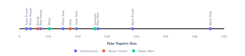
Figure 3: The different values for the False Negative Rate Parity measurement for the LSAC case study. Minority subgroups under intersectionality show a far greater range of disparity than what the binary metrics would suggest.

3.6.2 Attention

Attention is the exposure-based metric we discuss here. Ranking problems are unique from classification problems in the sense that the position of a ranked item, even within the top K results, can draw significantly different levels of visual attention. Previous research shows that people’s attention sharply drops off after the first few items in a ranked list Mullick et al. (2019). Different papers have modeled visual attention as a function of the position K as a logarithmic distribution Singh and Joachims (2018), a geometric distribution, or other sharply falling distributions with increasing rank Sapiezynski et al. (2019). Assuming the attention distribution function of an item to be Att(k), the mean attention per subgroup is defined as:

$$\text{MA}_{sg_{i}}=\frac{1}{|sg_{i}|}\sum_{k=1}^{|\tau|}\text{Att(k)}~{}\text{where}~{}sg_{k}^{\tau}=sg_{i}$$ (17)

And, using our worst case method, the attention ratio (AR) is defined as:

$$\text{AR}=\frac{\text{min}\{\text{MA}_{sg_{i}},\forall i\in N\}}{\text{max}\{\text{MA}_{sg_{i}},\forall i\in N\}}$$ (18)

4 Case Study and LSAC Dataset

As an example application of the framework described in this paper, we present a case study on a trained tensorflow model outputs on the Law School Admissions Council (LSAC) dataset, where the classifier predicts whether a candidate passed the bar exam. We calculated metrics for binary values where only race (Table 1) or only gender (Table 2) is examined for the false negative rates (FNR) and also for an intersectional FNR metric, where both race and gender are used (Table 3).

Race	FNR
nonwhite	0.025829
white	0.010230

Table 1: False negative rates using race

Gender	FNR
woman	0.006267
man	0.017384

Table 2: False negative rates using gender

Gender	Race	FNR
woman	asian	0.002398
woman	black	0.038700
woman	hisp	0.007246
woman	white	0.003802
man	asian	0.019512
man	black	0.065327
man	hisp	0.026804
man	white	0.014920

Table 3: False negative rates using intersectional race and gender subgroups.

The tables show clear examples of how viewing fairness metrics for only one group or protected class can obscure inequality for combined subgroups. When using only the gender lens, the FNR is lower for women, $\approx{0.006}$ when compared to men, $\approx{0.017}$ (Table 2). However the trend reverses for certain subgroups when race is added. For example with Black women having higher FNR at $\approx{0.039}$ when compared either to white men at $\approx{0.015}$ or asian men at $\approx{0.020}$ (Table 3). The min/max ratio is 0.002398/0.065327 = 0.036, which is far from the ideal value of 1. The model therefore fails to achieve intersectional fairness under FNR parity.

5 Discussion

5.1 Conclusion

In this paper, we introduce the worst-case comparison as a simple, easily comprehensible method to surface hidden biases that commonly used fairness metrics may not be able to show. We establish the importance of introducing such modifications to better serve minorities with sparse populations and show how the method can be applied to a diverse range of model metrics, thereby being easy for practitioners and researchers to adapt without significantly changing their existing fairness monitoring systems.

5.2 Limitations and Future Work

The idea of creating combinatorial subgroups has a couple of caveats: It does not take into account partial group membership (for instance, a person who identifies as multiracial), or continuous variables (for example, instead of treating age as an integer, we would convert the age attribute as discrete buckets). We encourage researchers to expand our method to include partial group membership and continuous attributes.

Secondly, creating a combinatorially large number of subgroups inevitably leads to subgroups which have a very small number of members, thereby demonstrating the effects of Simpson’s Paradox Blyth (1972). A possible direction of research could be to introduce statistical significance measures for such small subgroups, and suggest thumb rules for subgroup creation via empirical measurements.

The authors would like to thank Joshua Rubin, Amit Paka, Jack Reidy, Aalok Shanbhag, Christo Wilson, and the anonymous reviewers for their helpful discussions and suggestions.

References

- Berg (1964) Richard K Berg. Equal employment opportunity under the civil rights act of 1964. Brook. L. Rev., 31:62, 1964.
- Binns (2019) Reuben Binns. On the apparent conflict between individual and group fairness. CoRR, abs/1912.06883, 2019. URL http://arxiv.org/abs/1912.06883.
- Blyth (1972) Colin R Blyth. On simpson’s paradox and the sure-thing principle. Journal of the American Statistical Association, 67(338):364–366, 1972.
- Bockting et al. (2016) Walter Bockting, Eli Coleman, Madeline B Deutsch, Antonio Guillamon, Ilan Meyer, Walter Meyer III, Sari Reisner, Jae Sevelius, and Randi Ettner. Adult development and quality of life of transgender and gender nonconforming people. Current opinion in endocrinology, diabetes, and obesity, 23(2):188, 2016.
- Bogen and Rieke (2018) Miranda Bogen and Aaron Rieke. Help wanted: An examination of hiring algorithms, equity, and bias. 2018.
- Buolamwini and Gebru (2018) Joy Buolamwini and Timnit Gebru. Gender shades: Intersectional accuracy disparities in commercial gender classification. In Conference on fairness, accountability and transparency, pages 77–91, 2018.
- Commission et al. (1979) Equal Employment Opportunity Commission et al. Adoption of questions and answers to clarify and provide a common interpretation of the uniform guidelines on employee selection procedures. Federal Register, 44(43):11996–12009, 1979.
- Corbett-Davies and Goel (2018) Sam Corbett-Davies and Sharad Goel. The measure and mismeasure of fairness: A critical review of fair machine learning. arXiv preprint arXiv:1808.00023, 2018.
- Corbett-Davies et al. (2017) Sam Corbett-Davies, Emma Pierson, Avi Feller, Sharad Goel, and Aziz Huq. Algorithmic decision making and the cost of fairness. In Proceedings of the 23rd acm sigkdd international conference on knowledge discovery and data mining, pages 797–806, 2017.
- Crenshaw (1989) Kimberlé Crenshaw. Demarginalizing the intersection of race and sex: A black feminist critique of antidiscrimination doctrine, feminist theory and antiracist politics. u. Chi. Legal f., page 139, 1989.
- Dwork et al. (2012) Cynthia Dwork, Moritz Hardt, Toniann Pitassi, Omer Reingold, and Richard Zemel. Fairness through awareness. In Proceedings of the 3rd innovations in theoretical computer science conference, pages 214–226, 2012.
- Feldman et al. (2016) Jamie Feldman, George R Brown, Madeline B Deutsch, Wylie Hembree, Walter Meyer, Heino FL Meyer-Bahlburg, Vin Tangpricha, Guy T’Sjoen, and Joshua D Safer. Priorities for transgender medical and health care research. Current opinion in endocrinology, diabetes, and obesity, 23(2):180, 2016.
- Foulds et al. (2020) James R Foulds, Rashidul Islam, Kamrun Naher Keya, and Shimei Pan. An intersectional definition of fairness. In 2020 IEEE 36th International Conference on Data Engineering (ICDE), pages 1918–1921. IEEE, 2020.
- Gartner (2020) Joseph Gartner. A New Metric for Quantifying Machine Learning Fairness in Healthcare. %TT␣every␣character␣and␣hyphenate␣after␣it%****␣main.bbl␣Line␣100␣****https://closedloop.ai/a-new-metric-for-quantifying-fairness-in-healthcare/, 2020.
- Geyik et al. (2019) Sahin Cem Geyik, Stuart Ambler, and Krishnaram Kenthapadi. Fairness-aware ranking in search & recommendation systems with application to linkedin talent search. In Proceedings of the 25th ACM SIGKDD International Conference on Knowledge Discovery & Data Mining, pages 2221–2231, 2019.
- Goodman and Flaxman (2017) Bryce Goodman and Seth Flaxman. European union regulations on algorithmic decision-making and a “right to explanation”. AI magazine, 38(3):50–57, 2017.
- Hardt et al. (2016) Moritz Hardt, Eric Price, and Nati Srebro. Equality of opportunity in supervised learning. In Advances in neural information processing systems, pages 3315–3323, 2016.
- Hébert-Johnson et al. (2018) Úrsula Hébert-Johnson, Michael Kim, Omer Reingold, and Guy Rothblum. Multicalibration: Calibration for the (computationally-identifiable) masses. In International Conference on Machine Learning, pages 1939–1948, 2018.
- Kearns et al. (2018) Michael Kearns, Seth Neel, Aaron Roth, and Zhiwei Steven Wu. Preventing fairness gerrymandering: Auditing and learning for subgroup fairness. In International Conference on Machine Learning, pages 2564–2572. PMLR, 2018.
- Kim et al. (2019) Michael P Kim, Amirata Ghorbani, and James Zou. Multiaccuracy: Black-box post-processing for fairness in classification. In Proceedings of the 2019 AAAI/ACM Conference on AI, Ethics, and Society, pages 247–254, 2019.
- King et al. (2009) Malcolm King, Alexandra Smith, and Michael Gracey. Indigenous health part 2: the underlying causes of the health gap. The lancet, 374(9683):76–85, 2009.
- Kusner et al. (2017) Matt J Kusner, Joshua Loftus, Chris Russell, and Ricardo Silva. Counterfactual fairness. In Advances in neural information processing systems, pages 4066–4076, 2017.
- Mary et al. (2019) Jérémie Mary, Clément Calauzènes, and Noureddine El Karoui. Fairness-aware learning for continuous attributes and treatments. In International Conference on Machine Learning, pages 4382–4391, 2019.
- Mehrabi et al. (2019) Ninareh Mehrabi, Fred Morstatter, Nripsuta Saxena, Kristina Lerman, and Aram Galstyan. A survey on bias and fairness in machine learning. CoRR, abs/1908.09635, 2019. URL http://arxiv.org/abs/1908.09635.
- Mukerjee et al. (2002) Amitabha Mukerjee, Rita Biswas, Kalyanmoy Deb, and Amrit P Mathur. Multi–objective evolutionary algorithms for the risk–return trade–off in bank loan management. International Transactions in operational research, 9(5):583–597, 2002.
- Mullick et al. (2019) Ankan Mullick, Sayan Ghosh, Ritam Dutt, Avijit Ghosh, and Abhijnan Chakraborty. Public sphere 2.0: Targeted commenting in online news media. In European Conference on Information Retrieval, pages 180–187. Springer, 2019.
- Paradies (2006) Yin Paradies. A systematic review of empirical research on self-reported racism and health. International journal of epidemiology, 35(4):888–901, 2006.
- Rawls (2001) John Rawls. Justice as fairness: A restatement. Harvard University Press, 2001.
- Reisner et al. (2016) Sari L Reisner, Madeline B Deutsch, Shalender Bhasin, Walter Bockting, George R Brown, Jamie Feldman, Rob Garofalo, Baudewijntje Kreukels, Asa Radix, Joshua D Safer, et al. Advancing methods for us transgender health research. Current opinion in endocrinology, diabetes, and obesity, 23(2):198, 2016.
- Sapiezynski et al. (2019) Piotr Sapiezynski, Wesley Zeng, Ronald E Robertson, Alan Mislove, and Christo Wilson. Quantifying the impact of user attentionon fair group representation in ranked lists. In Companion Proceedings of The 2019 World Wide Web Conference, pages 553–562, 2019.
- Singh and Joachims (2018) Ashudeep Singh and Thorsten Joachims. Fairness of exposure in rankings. In Proceedings of the 24th ACM SIGKDD International Conference on Knowledge Discovery & Data Mining, pages 2219–2228, 2018.
- Vasilescu and Terzopoulos (2002) M Alex O Vasilescu and Demetri Terzopoulos. Multilinear image analysis for facial recognition. In Object recognition supported by user interaction for service robots, volume 2, pages 511–514. IEEE, 2002.
- Veen et al. (2018) Duco Veen, Diederick Stoel, Naomi Schalken, Kees Mulder, and Rens Van de Schoot. Using the data agreement criterion to rank experts’ beliefs. Entropy, 20(8):592, 2018.
- Verma and Rubin (2018) Sahil Verma and Julia Rubin. Fairness definitions explained. In Proceedings of the International Workshop on Software Fairness, FairWare ’18, page 1–7, New York, NY, USA, 2018. Association for Computing Machinery. ISBN 9781450357463. 10.1145/3194770.3194776. URL https://doi.org/10.1145/3194770.3194776.
- Yang and Stoyanovich (2017) Ke Yang and Julia Stoyanovich. Measuring fairness in ranked outputs. In Proceedings of the 29th International Conference on Scientific and Statistical Database Management, pages 1–6, 2017.