Numerically exact open quantum systems simulations for arbitrary environments using automated compression of environments

Abstract

The central challenge for describing the dynamics in open quantum systems is that the Hilbert space of typical environments is too large to be treated exactly. In some cases, such as when the environment has a short memory time or only interacts weakly with the system, approximate descriptions of the system are possible. Beyond these, numerically exact methods exist, but these are typically restricted to baths with Gaussian correlations, such as non-interacting bosons. Here we present a numerically exact method for simulating open quantum systems with arbitrary environments which consist of a set of independent degrees of freedom. Our approach automatically reduces the large number of environmental degrees of freedom to those which are most relevant. Specifically, we show how the process tensor—which describes the effect of the environment—can be iteratively constructed and compressed using matrix product state techniques. We demonstrate the power of this method by applying it to problems with bosonic, fermionic, and spin environments: electron transport, phonon effects and radiative decay in quantum dots, central spin dynamics, anharmonic environments, dispersive coupling to time-dependent lossy cavity modes, and superradiance. The versatility and efficiency of our automated compression of environments (ACE) method provides a practical general-purpose tool for open quantum systems.

An inevitable property of quantum technologies is that quantum devices interact with their environment [1]. This interaction gives rise to dephasing and dissipation but, if understood, it can be exploited for example in environment-assisted quantum transport [2, 3, 4], or even quantum information processing [5, 6]. Because of the exponential growth of Hilbert space dimension, and the large number of environmental degrees of freedom, the direct solution of Schrödinger’s equation for system and environment is usually infeasible. As such, one requires practical methods that allow simulation of the dynamics of the system, while accounting for effects of the environment [1, 7, 8, 9].

Among such approaches, those most frequently used rely on the Born and Markov approximations, which enable one to derive time-local equations of motion for the reduced system density matrix [1, 10]. The Born approximation implies that the environment does not change significantly with time—i.e. that system-environment correlations are weak and transient. While valid for weakly coupled open quantum systems, other environments lead to strong system-environment correlations [11]. The Markov approximation depends on the memory time of the environment being short compared to the time evolution of the system. This fails if the spectral density is highly structured, or if there is a long memory time [12]. Given these widespread limitations, approaches beyond the Born–Markov approximation are clearly necessary.

Figure 1: Depiction of the automated compression of environments approach. a, The identification of an efficient representation is fully automatic and does not rely on any a priori approximations or assumptions. b, The time evolution of system plus its compressed environment proceeds in discrete time steps. Information flow is indicated by the coloured arrows. c, Formally, the general propagation of a quantum system can be expressed with a process tensor $\mathcal{I}$. d, Propagation with a process tensor in MPO form: this corresponds to the schematic situation depicted in panel b. e, Combination of the influence of environment mode $K$ with the process tensor containing the influences of modes $1,2,\dots,K-1$. Red semicircles indicate the effects of the MPO compression (as depicted schematically in panels a and b).

Numerically exact methods—where tuning convergence parameters allows one to trade off precision against computation time—do exist for some non-Markovian problems: those where the environments have Gaussian correlations, such as non-interacting bosonic modes. Such methods include hierarchical equations of motion (HEOM) [13, 14], chain mapping through orthogonal polynomials [15, 16, 17], or the Feynman-Vernon real-time path integral formalism [18]. In particular, the iterative form of the path integral [19, 20, 21] and its reformulation with matrix product operators [22] have been used successfully, e.g., to simulate phonon effects on spectra [23, 24], to devise robust and high-fidelity protocols for the emission of nonclassical light [25, 26, 27], and to model concrete experiments on optically driven quantum dots [28, 29, 30]. Such approaches have been extended to systems with multiple environments [31], to multi-level systems [21], and to special types of non-Gaussian baths such as quadratic coupling to bosons or fermions [32]. Some methods for general environments do exist, such as correlation expansion [33], but it is complicated to derive these equations at higher expansion order. As such, a challenge remains: to provide general and efficient numerically exact methods which can also model non-Gaussian non-Markovian environments.

Here we provide such a method, which can be used to simulate open quantum systems coupled to arbitrary environments (see Fig. 1a). We demonstrate its practical application with a variety of forms of environment—bosonic, fermionic, and spins. Because the derivation is general the same code can be used to simulate the dynamics of a large variety of different physical systems. At the core of our automated compression of environments (ACE) method is the explicit microscopic construction of the process tensor (PT) [34, 35]—an object originally conceived as a way to conceptualize correlations for a general non-Markovian environment—and a route to efficiently compress this object using matrix product operator (MPO) techniques [36, 37]. Specifically, we provide a general and efficient algorithm to directly construct an MPO representation of the PT, corresponding to an automated projection of the environment onto its most relevant degrees of freedom.

Results

.1 Automated compression of environments

The working principle of ACE is to represent the environment efficiently by concentrating on its most relevant degrees of freedom (cf. Fig. 1a). These are selected automatically using MPO compression techniques and may differ from one time step to another. This procedure guarantees fully capturing the non-Markovian information flow from past time steps to later time steps via the environment (cf. Fig. 1b). We now summarise the ACE method introduced in this paper; further details are provided in the Methods section. Our goal is to obtain the reduced system density matrix $\rho_{\nu\mu}(t)$ at a time $t$, accounting for coupling to a given environment. We discretise the time axis on a grid $t_{l}=l\Delta t$ with equal time steps $\Delta t$ (Fig. 1b-d); then, for a single time step, the time evolution operator $U(\Delta t)=e^{-\frac{i}{\hbar}H\Delta t}$ of the total system can be factorised using the Trotter expansion $U(\Delta t)=e^{-\frac{i}{\hbar}H_{E}\Delta t}e^{-\frac{i}{\hbar}H_{S}\Delta t}+\mathcal{O}(\Delta t^{2})$, where the total Hamiltonian $H=H_{S}+H_{E}$ is decomposed into the system Hamiltonian $H_{S}$ and the environment Hamiltonian $H_{E}$ including the system-environment coupling. Inserting a complete set of basis states for the system and the environment and tracing out the environment, the reduced system density matrix at time $t_{n}$ can be written

$$\rho_{\alpha_{n}}=\sum_{\begin{subarray}{c}\alpha_{n-1}\dots\alpha_{0}\\ \tilde{\alpha}_{n}\dots\tilde{\alpha}_{1}\end{subarray}}\mathcal{I}^{(\alpha_{n}\tilde{\alpha}_{n})\dots(\alpha_{1}\tilde{\alpha}_{1})}\bigg{(}\prod_{l=1}^{n}\mathcal{M}^{\tilde{\alpha}_{l}\alpha_{l-1}}\bigg{)}\rho_{\alpha_{0}},$$ (1)

where we have defined $\alpha=(\nu,\mu)$ to combine two Hilbert space indices into a single Liouville space index. A visual representation of Eq. (1) is depicted in Fig. 1c. Here, $\mathcal{M}$ describes the free propagation of the system. This can be time-dependent, and can additionally include effects of Markovian baths. The effects of the general non-Markovian non-Gaussian environment are captured in the quantity $\mathcal{I}$, which we refer to as the process tensor (PT). This object differs slightly from the original definition of the PT [35], in that we have separated out the initial state and the free system evolution. When $\mathcal{I}$ is non-zero only for diagonal couplings $\alpha_{l}=\tilde{\alpha}_{l}$ this object becomes equivalent to the Feynman-Vernon influence functional [18]. The PT can thus be considered as a generalisation of this influence functional to the case of non-diagonal couplings. From the explicit expression for the PT we find that it automatically has the form of an MPO:

$$\mathcal{I}^{(\alpha_{n},\tilde{\alpha}_{n})(\alpha_{n-1},\tilde{\alpha}_{n-1})\dots(\alpha_{1},\tilde{\alpha}_{1})}=$$

$$\sum_{d_{n-1}\dots d_{1}}\mathcal{Q}_{1d_{n-1}}^{(\alpha_{n},\tilde{\alpha}_{n})}\mathcal{Q}_{d_{n-1}d_{n-2}}^{(\alpha_{n-1},\tilde{\alpha}_{n-1})}\dots\mathcal{Q}_{d_{1}1}^{(\alpha_{1},\tilde{\alpha}_{1})}.$$ (2)

Here the dimension of the inner indices $d_{l}$ is very large, corresponding to a complete basis of environment states in Liouville space. This large dimension precludes the direct application of Eqs. (1) and (2) for typical environments. However, the MPO form of the PT means it is in principle amenable to standard MPO compression, based on singular value decomposition as described in the Methods [36, 37]. Such compression corresponds physically to reducing the environment to its most relevant degrees of freedom, which, as theoretical consideration of PTs suggest [38], may be few in number.

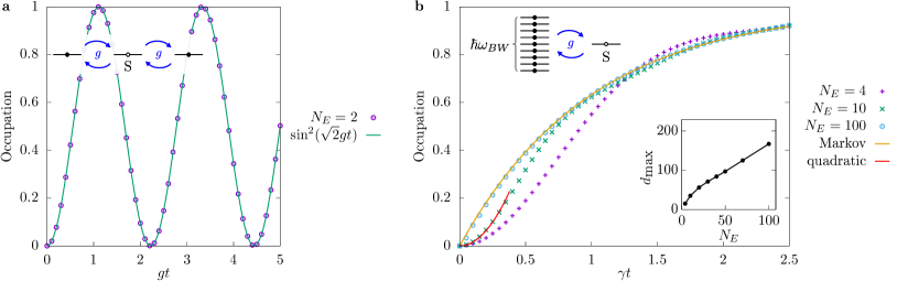
Figure 2: Resonant-level model application of ACE, spanning small to infinite bath memory time. a, Dynamics of the occupations of a single localised quantum state (S) coupled to two resonant environment modes. b, Dynamics of a quantum state coupled to a quasi-continuum of modes. ACE simulations (points) are shown together with analytic solutions (lines). In b, the analytic result in the Markov limit corresponds to an exponential transfer with the rate obtained from Fermi’s golden rule. The result of a quadratic Taylor expansion around $t=0$ is depicted for the case $N_{E}=10$. The top left insets depict the respective physical situations. The bottom right inset in b shows the maximal inner dimension $d_{\textrm{max}}$ of the PT MPO as a function of the number of environment states $N_{E}$ for constant density of states.

The key challenge is thus to find an efficient way to calculate the compressed form of the PT MPO, without first constructing the uncompressed PT. This can be achieved through the ACE approach, for any problem with an environment that can be decomposed into $N_{E}$ different noninteracting degrees of freedom:

$$H=H_{S}+\sum_{k=1}^{N_{E}}H_{E}^{k}.$$ (3)

The label $k$ can describe both the different degrees of freedom within a bath (e.g. different spins, or photon modes defined by their wave vector $\mathbf{q}$), but can also enumerate multiple environments coupled to the same system. In all of these cases, the PT can be constructed iteratively, by adding successively the contribution of each bath degree of freedom. The process of combining the influence of the $K$-th degree of freedom, $\mathcal{B}[K]$, with an existing PT MPO $Q[K-1]$ is shown in Fig. 1e. If the resulting MPOs are compressed after each step (red semicircles), the inner dimension remains manageable and exact diagonalisation can be used for the singular value decomposition. This is described in more detail in the Methods section.

Once one has the compressed PT in MPO representation, this can be substituted into Eq. (1). The calculation of the reduced system density matrix then amounts to the contraction of a network of the form shown in Fig. 1d. If the PT MPO has a sufficiently small inner dimension, this contraction is straightforward. Because this algorithm can be applied in principle to arbitrary environments simply by specifying the respective environment Hamiltonians $H_{E}^{k}$, ACE allows investigations of a huge variety of different open quantum systems. We next show how this method works in practice for a few paradigmatic example problems.

.2 Resonant-level model

As a first test of ACE, we consider the archetypal problem of electron transport between a single localised electron state and other nearby environment states, described by the resonant-level model. The $k$-th environment state is described by

$$H_{E}^{k}= \hbar\omega_{k}c^{\dagger}_{k}c_{k}+\hbar g_{k}(c^{\dagger}_{k}c_{S}+c^{\dagger}_{S}c_{k}),$$ (4)

where $c^{\dagger}_{S}(c_{S})$ and $c_{k}^{\dagger}(c_{k})$ create (destroy) a fermion in the localised system state and the $k$-th environment state, respectively, $\hbar\omega_{k}$ is the energy of the $k$-th environment state with respect to the system state, and $g_{k}$ is the coupling constant, which we assume to be independent of $k$, $g_{k}=g$. The free system Hamiltonian is $H_{S}=0$. The Hamiltonian in Eq. (4) shows distinct behaviour depending on the number of environment modes: coherent oscillations for few modes, and irreversible decay for a broad continuum of modes. In the following we show that ACE can automatically capture both these limits, and interpolate between them.

For a few environment modes, the dynamics is described by coherent oscillations at the eigenfrequencies of the coupled system and environment. Here, we consider the situation depicted in the inset of Fig. 2a where a single initially empty site is connected to two sites at the same energy $\omega_{k}=0$, which are initially occupied. In this scenario the time-dependent many-body state of the total system is

$$|\Psi(t)\rangle= \bigg{[}\cos(\sqrt{2}gt)\frac{c^{\dagger}_{1}+c^{\dagger}_{2}}{\sqrt{2}}-i\sin(\sqrt{2}gt)c^{\dagger}_{S}\bigg{]}\frac{c^{\dagger}_{1}-c^{\dagger}_{2}}{\sqrt{2}}|0\rangle.$$ (5)

In Figure 2a, we compare the occupation $n_{S}=\sin^{2}(\sqrt{2}gt)$ to the results of ACE simulations for convergence parameters $\Delta t=0.01g$ and $\epsilon=10^{-7}$ (see Methods). We see the results match perfectly. Since the oscillations are undamped, the memory time of the environment is infinite. Furthermore, whenever $n_{S}=\frac{1}{2}$, Eq. (5) describes a state with maximal entanglement between system and environment. This demonstrates that ACE can account for infinite memory times as well as strong system-environment correlations.

Different behaviour occurs for a quasi-continuum of environment states, e.g., metallic leads coupled to a quantum dot [39], as depicted in the top left inset of Fig. 2b. The oscillatory contributions of the different modes interfere destructively, suppressing oscillations. When the continuum is broad enough, there is a short memory time and weak system-bath correlations, so the situation is well described by Markovian master equations. These predict charge transfer to the localised state at a rate $\gamma=2\pi\hbar g^{2}D$, where $D=(N_{E}-1)/(\hbar\omega_{BW})$ is the density of states and $\hbar\omega_{BW}$ is the bandwidth. Figure 2b shows the corresponding dynamics for different numbers of environment modes $N_{E}$ with a fixed density of states $D=1/(\hbar\gamma)$. As the number of environment modes (and therefore the bandwidth) increases, the simulations approach the Markovian analytic result $1-\exp(-\gamma t)$. For intermediate $N_{E}=10$, the finite bandwidth introduces a finite memory time $\sim 1/\omega_{BW}$. To check the validity of the ACE results in this more complicated crossover regime, we also plot the analytic short-time Taylor expansion, $n_{S}\approx\gamma\omega_{BW}t^{2}/(2\pi)$ for the case $N_{E}=10$.

The inset in Fig. 2b shows the maximal inner dimension $d_{\textrm{max}}$ of the PT MPO as a function of the number of modes $N_{E}$. We see this scales linearly with the number of modes, indicating a very efficient reduction, compared to the exponential scaling of the dimension of the full environment Liouville space of up to $4^{100}\approx 1.6\times 10^{60}$ for $N_{E}=100$. A more detailed analysis of numerical convergence is given in the Supplemental Material S.2. This simple example demonstrates that ACE is able to reproduce analytic results in all regimes from infinite memories to Markovian environments and from strong to weak system-environment correlations.

.3 Simultaneous coupling of quantum dots to phonons and electromagnetic field modes

Our second example involves a system coupled simultaneously to two structured baths, as exemplified by a semiconductor quantum dot, coupled both to acoustic phonons and an electromagnetic environment. The acoustic phonon modes couple via a pure-dephasing interaction:

$$H_{\textrm{ph}}^{\mathbf{q}}= \hbar\omega_{\mathbf{q}}b^{\dagger}_{\mathbf{q}}b_{\mathbf{q}}+\hbar\gamma_{\mathbf{q}}\big{(}b^{\dagger}_{\mathbf{q}}+b_{\mathbf{q}}\big{)}|X\rangle\langle X|,$$ (6)

where $b^{\dagger}_{\mathbf{q}}$ ($b_{\mathbf{q}}$) creates (annihilates) a phonon with wave vector $\mathbf{q}$ and $|X\rangle$ denotes the exciton state of the quantum dot. If this were the only interaction, its linear and diagonal structure would mean it could be treated within the iterative quasi-adiabatic path integral (iQUAPI) method [19, 21, 23]. We will use this below to compare the results of ACE to that of iQUAPI.

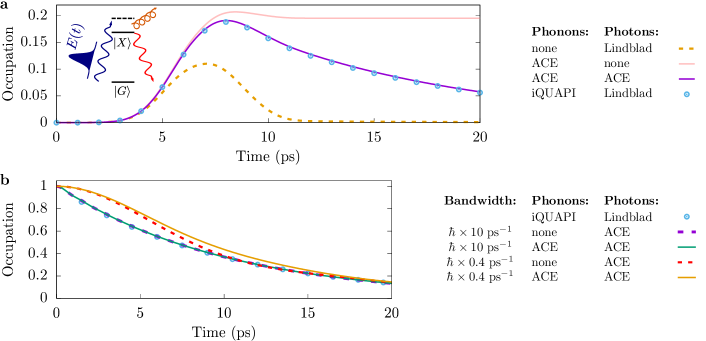
Figure 3: Dynamics of quantum dots embedded in (non-additive) photon and phonon environments. a, Dynamics of the exciton occupation for phonon-assisted off-resonant excitation of a QD driven by a Gaussian laser pulse and subject to radiative decay according to different theoretical approaches: The QD-phonon interaction may be disregarded (none) or treated within ACE or iQUAPI. The coupling between the QD and the photonic modes may be disregarded (none), included explicitly in ACE via its Hamiltonian, or replaced by a Lindblad term for radiative decay. b, Radiative decay of an initially occupied exciton state with and without interactions with phonons for model photon densities of states with different bandwidths $\hbar\omega_{BZ}$.

In addition to the bath of phonons, QDs also couple to the continuum of electromagnetic modes, which are responsible for radiative decay. Here the interaction with photon mode $k$ takes the Jaynes-Cummings form:

$$H_{JC}^{k}= \hbar\omega_{k}a^{\dagger}_{k}a_{k}+\hbar g_{k}\big{(}a^{\dagger}_{k}|G\rangle\langle X|+a_{k}|X\rangle\langle G|\big{)},$$ (7)

where $a^{\dagger}_{k}$ ($a_{k}$) is the bosonic creation (annihilation) operator for a photon in mode $k$.

There are several ways of including both baths in simulations: First, for unstructured (i.e. Markovian) photon environments, the Born–Markov approximation holds, so we can account for the radiative decay as a Lindblad term, $\kappa\mathcal{L}\big{[}|G\rangle\langle X|,\rho\big{]}$ where

$$\mathcal{L}\big{[}|G\rangle\langle X|,\rho\big{]}\\ \equiv|G\rangle\langle X|\rho|X\rangle\langle G|-\tfrac{1}{2}\big{(}|X\rangle\langle X|\rho+\rho|X\rangle\langle X|\big{)}.$$ (8)

In both ACE and iQUAPI [40], such Markovian dissipation can be included into the free system Liouville propagator $\mathcal{M}$. Due to the flexibility of ACE, we can also describe the radiative decay microscopically by including both the phonon and electromagnetic environments in the PT. This has the advantage that it automatically captures possible non-additive effects of the simultaneous coupling to multiple baths [41, 42, 43], and also allows one to extend to structured electromagnetic environments.

In Fig. 3a, we show how the occupation of a QD responds to off-resonant excitation by a Gaussian laser pulse. This drive corresponds to the following time-dependent Hamiltonian in the rotating frame of the laser:

$$H_{S}=-\hbar\delta|X\rangle\langle X|+\tfrac{\hbar}{2}\Omega(t)\big{(}|X\rangle\langle G|+|G\rangle\langle X|\big{)},$$ (9)

where $\delta$ is the laser detuning and $\Omega(t)$ is a Gaussian envelope centred at $t_{0}=7$ ps with pulse duration $\tau_{\textrm{FWHM}}=5$ ps. The QD simultaneously interacts with the phonon and photon baths, which are treated within different theoretical approaches. In this figure we assume a flat electromagnetic environment, so all approaches should work equally well. The simulation parameters are summarised in the Methods section.

In the absence of QD-phonon interactions, the exciton is only occupied transiently during the pulse, as absorption is suppressed by the detuning of the laser from the exciton energy. Including phonons within ACE but disregarding radiative decay entirely results in a nonzero stationary exciton occupation, as the detuning may be bridged by phonon emission. Including both phonons and photons, one sees absorption followed by radiative decay. Identical results are found for this case for both ACE—treating the electromagnetic environment microscopically—and for iQUAPI with photon decay $\kappa\mathcal{L}\big{[}|G\rangle\langle X|,\rho\big{]}$. As such, we both further confirm the capabilities of ACE, and see that—as may be anticipated—for an unstructured photon environment, no cross-action between the coupling to photon and phonon baths can be identified.

As already noted, ACE is also able to treat situations with non-additive environments, as is relevant for structured photonic environments like waveguides or microcavities [44, 45]. Figure 3b shows the decay of an initially occupied exciton state (with $H_{S}=0)$ where, in addition to the non-Markovian phonon bath, we use a photon bath with a finite bandwidth $\hbar\omega_{BW}$. For large bandwidths, no cross-interaction between the couplings to the two baths is found (and so the results again match iQUAPI with Lindbladian photon loss). For small bandwidths $\omega_{BW}=0.4$ ps^-1, the photon environment obtains a memory time $\tau\sim 1/\omega_{BW}$ of the same order of magnitude as the phonon environment. As a result the two baths couple non-additively, as can be seen by the fact that the coupling to phonons significantly influences the decay of excitations into the electromagnetic modes.

.4 Spin dynamics

Our third example concerns the spin dynamics in the presence of a spin environment [46, 47]. Besides demonstrating the applicability of ACE to non-Gaussian spin environments, this example also identifies the limits on efficient environment compression. We consider a central spin coupled to a bath of environment spins by a Heisenberg interaction

$$H_{E}^{k}= \frac{J_{k}}{\hbar^{2}}\,\hat{\mathbf{S}}\cdot\hat{\mathbf{s}}_{k},$$ (10)

where $\hat{\mathbf{S}}$ and $\hat{\mathbf{s}}_{k}$ are the spin-$\frac{1}{2}$ operators of the central spin and the $k$-th environment spin, respectively—see inset of Fig. 4. In the following we choose the coupling constants $J_{k}=J/N$, where $N$ is the number of environment spins and $J$ defines the energy scale of the coupling. We set $H_{S}=0$ and initially prepare the system spin in the state with maximal $\langle S_{x}\rangle$. We then explore how the initial degree of polarisation of the environment affects the system dynamics, and the ability to efficiently compress the environment.

Figure 4: Central spin model for different degrees of spin bath polarisation. Dynamics of a central spin (red) initially prepared along the $x$-axis in a bath of $N$ spins (blue) as depicted in the insets. The $x$-component of a central spin is shown for situations where the bath spins are fully polarised a, partially polarised b, or unpolarised c. The number of environment spins $N$ is varied keeping the sum of the couplings $\sum_{k}J_{k}=J$ constant. Colours correspond to different numbers of environment spins $N$ while point types correspond to different values of the MPO compression threshold $\epsilon$.

First, we focus on the situation where the environment spins are completely polarised along the $z$-axis. The respective dynamics of $\langle S_{x}\rangle$ is depicted in Fig. 4a for different numbers of environment spins $N=10$, $N=100$, and $N=1000$ and for convergence parameters $\Delta t=0.01\hbar/J$ and $\epsilon=10^{-10}$. The Heisenberg coupling leads to a coherent precession of the system and environment spins about each other. In the limit $N\to\infty$, there is no back-action on the environment so the environment remains in its initial state. The dynamics is then equivalent to a precession about a constant effective magnetic field, for which $\langle S_{x}\rangle=(\hbar/2)\cos\big{[}(tJ)/(2\hbar)\big{]}$. We see the ACE simulations for $N=1000$ approach this limit. It is noteworthy that for all $N$ the inner dimension of the PT MPO remains 4, corresponding to the Liouville space dimension of a single spin $\frac{1}{2}$. This is because all environment spins behave identically, so the environment can be replaced by a single effective spin.

We next explore the limitations of compression of the environment, by considering randomised initial conditions for the environment spins. In Fig. 4b and c we present ACE simulations with $N=10$ and $N=100$ environment spins for different values of the MPO truncation threshold $\epsilon$. In Fig. 4b the bath is partially polarised: we randomly select pure spin states from an isotropic distribution and filter these with a rejection probability $1-\exp\big{[}b\big{(}s^{z}_{k}/\hbar-\tfrac{1}{2}\big{)}\big{]}$. Here, $b=(g\mu_{B}B)/(k_{B}T)$ is a Boltzmann factor, taken as $b=20$ for Fig. 4b. In Fig. 4c we instead use a uniform distribution (i.e. $b=0$). In both cases a dephasing of the central spin is visible. However, for the unpolarised case, the spin dynamics for different $\epsilon$ start to diverge at long times. The slow convergence with $\epsilon$ in this situation is a consequence of the intrinsic incompressibility of the environment degrees of freedom. That is, because each environment spin reacts differently to the system spin, the joint PT cannot be compressed efficiently. Furthermore, environment spins can become correlated via an effective interaction mediated by the system, and without an external magnetic field the environment states are highly degenerate. Consequently, there is no clear physical constraint on the accessible environment Hilbert space. In the partially polarised case, the environment can be compressed more efficiently, so that the ACE simulations show a better convergence.

.5 Anharmonic environments

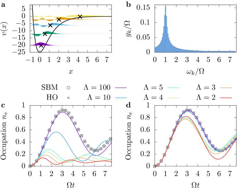
Figure 5: Two-level system coupled to a bath of anharmonic modes. a: Morse potential, Eq. (11), with parameter $\Lambda=5$ and its bound eigenstates obtained numerically. Crosses mark the average position $\langle i|\hat{x}|i\rangle$ for each eigenstate. b: Coupling coefficients $g_{k}$ corresponding to a Lorentzian spectral density of environment modes. c: ACE simulations with $M=\min\{5,\Lambda\}$ environment levels for: the spin-boson model (SBM), harmonic oscillator (HO) modes obtained by the finite differences method, and finite differences solutions of the Morse potential for different $\Lambda$. d: Analogous calculations to c but where energy shifts due to non-zero $\langle i|\hat{x}|i\rangle$ have been subtracted.

While a bath of harmonic oscillators forms a Gaussian environment, which can be addressed by a multitude of existing numerically exact methods, anharmonic environment modes have so far been out of reach. Anharmonicities are found in practice, e.g., in vibrational modes of molecules with a finite number of bound vibrational states, commonly modelled by a Morse potential [48]

$$v(x)= \Lambda^{2}\Big{(}e^{-2x}-2e^{-x}\Big{)},$$ (11)

where $\Lambda$ controls the depth of the potential and number of bound states. Here, we use the Morse potential as a demonstration of simulating environment modes with arbitrary potentials $v(x)$.

As described in more detail in the Supplementary Material S.4, we first use a finite differences method to numerically find the eigenstates of a single uncoupled environment mode, before introducing coupling to the system. For example, the bound eigenstates of the Morse potential for $\Lambda=5$ are depicted in Fig. 5a. Keeping only the $M$ lowest energy eigenstates and choosing a system-environment coupling proportional to the environment position operator, we find that for environment mode $k$

$$H_{E}^{k}= \sum_{j=0}^{M-1}\hbar\omega_{k}\tilde{E}_{j}\sigma^{k}_{jj}+\hbar g_{k}\sum_{i,j=0}^{M-1}\!\sqrt{2}\langle i|\tilde{x}|j\rangle\sigma^{k}_{ij}\,|e\rangle\langle e|,$$ (12)

where $\tilde{E}_{j}$ and $\langle i|\tilde{x}|j\rangle$ are scaled so that the spin-boson model Hamiltonian is recovered when $v(x)$ is the harmonic oscillator potential.

ACE simulations are performed for $H_{S}=\tfrac{\hbar}{2}\Omega\big{(}|e\rangle\langle g|+|g\rangle\langle e|\big{)}$, describing a continuously driven system performing Rabi oscillations damped by the anharmonic environment. We choose a set of $\omega_{k}$ and $g_{k}$ that correspond to a Lorentzian spectral density as shown in Fig. 5b; for other parameters see Supplementary Material S.4. The resulting excited state occupations $n_{e}$ are shown in Fig. 5c.

As a validity check, we first apply the above method to a harmonic potential, and recover exactly the dynamics of the spin-boson model. On moving to Morse potential environments, we find significant differences, especially for small $\Lambda$. Much of the difference is due to the asymmetry of the Morse potential, leading to an average position $\langle i|\tilde{x}|i\rangle$ that increases for higher excited states, indicated as crosses in Fig. 5a. This enters in $H_{E}$ via the system-environment coupling and results in an energy shift of the $|e\rangle$ system state. To better identify intrinsic effects of anharmonicity, Fig. 5d shows ACE results where this shift has been subtracted. For small $\Lambda$, one sees effects of the anharmonicity of the Morse potential, while for large $\Lambda$ the anharmonicity becomes negligible and the result of the Gaussian simulations is recovered.

Discussion
We have presented a novel, numerically exact, efficient, and versatile method: automated compression of environments (ACE), which makes it possible to simulate the dynamics of $N$-level quantum systems coupled to arbitrary environments directly from the microscopic system-environment coupling Hamiltonian. We have illustrated the power of this method with examples of electron transport, the simultaneous interaction of a QD with phonon and photon modes, spin dynamics, and anharmonic environments. In the Supplementary Material S.5, we provide an example exploring superradiant decay, illustrating that ACE can handle higher-dimensional system Hilbert spaces. Supplementary Material S.6 further contains an example of simulations of dispersive system-environment couplings as well as time-dependent driving and non-Hamiltonian loss terms acting directly on the environment. We have shown that ACE reproduces exact results in limiting cases, and can interpolate between infinite and short memory scenarios within the same algorithm. In particular, non-Markovian effects, system-environment correlations, and non-Gaussian baths are fully accounted for.

A fundamental restriction of ACE is that the environment must decompose into a set of separate modes without interactions between these modes. However, most typical models of open system environments satisfy this requirement. Moreover, recent work by [49] shows that, adapting a method of [50], one can extend tensor network methods to models where bath modes have nearest-neighbour interactions. Some environments have particular features that enable more specialised methods to be used, and these can be more efficient than the general method ACE. For example, Gaussian baths with a broad continuum of modes have short memory times at high temperature, and then iQUAPI [19] extremely efficient. In contrast, for environments consisting of only a few discrete modes, ACE outperforms methods based on Gaussian path integrals (see Supplementary Material S.3). For spectral densities with several peaks on top of a broad background, the construction of a PT for Gaussian environments in Ref. 34 can be readily combined with ACE to enable a hybrid approach within the common process tensor framework.

However, the unique feature of ACE is its generality. It can be used in situations where no specialised methods are available, and no new derivations or modifications of the algorithm are required when a new system or environment are considered. Due to its numerical exactness, ACE can serve as a benchmark for approximate methods which may provide a more tangible interpretation of physical processes, or serve a “turnkey solution” to simulate concrete experiments. These features make ACE a valuable general-purpose tool for open quantum systems.

Methods

.6 Derivation of the process tensor

We consider an arbitrary open quantum system specified by the Hamiltonian $H=H_{S}+H_{E}$, where $H_{S}$ is the free system Hamiltonian without coupling to the environment. For simplicity of notation we assume a time-independent Hamiltonian in the following, but generalisation to the time-dependent case is straightforward. The time evolution of the system density operator $\hat{\rho}_{S}$ can be obtained from the time evolution operator $U(t)$ of the total system, including the environment, by tracing out the environment to give:

$$\hat{\rho}_{S}(t)= \textrm{Tr}_{E}\Big{[}U(t)\big{(}\hat{\rho}_{S}(0)\otimes\hat{\rho}_{E}(0)\big{)}U^{\dagger}(t)\Big{]}.$$ (13)

We discretise the time evolution operator $U(t)=\prod_{l=1}^{n}U(\Delta t)$ on a time grid $t_{l}=l\Delta t$, $l=1\ldots n$ and apply a Trotter decomposition $U(\Delta t)=e^{-\frac{i}{\hbar}H_{E}\Delta t}\;e^{-\frac{i}{\hbar}H_{S}\Delta t}+\mathcal{O}(\Delta t^{2}).$ Next, we introduce a complete basis for the system ($\nu$ or $\mu$) as well as for the full environment ($\xi$ or $\eta$). We then introduce the matrix elements

$$A^{\nu_{l}\tilde{\nu}_{l}}_{\xi_{l}\xi_{l-1}}= \langle\nu_{l},\xi_{l}|e^{-\frac{i}{\hbar}H_{E}\Delta t}|\tilde{\nu}_{l},\xi_{l-1}\rangle,$$ (14)

$$M^{\tilde{\nu}_{l}\nu_{l-1}}= \langle\tilde{\nu}_{l}|e^{-\frac{i}{\hbar}H_{S}\Delta t}|\nu_{l-1}\rangle,$$ (15)

and, using calligraphic symbols, their counterparts in Liouville space:

$$\mathcal{A}^{(\nu_{l},\mu_{l}),(\tilde{\nu}_{l},\tilde{\mu}_{l})}_{(\xi_{l},\eta_{l}),(\xi_{l-1},\eta_{l-1})}:= A^{\nu_{l}\tilde{\nu}_{l}}_{\xi_{l}\xi_{l-1}}A^{\mu_{l}\tilde{\mu}_{l}*}_{\eta_{l}\eta_{l-1}}$$ (16)

$$\mathcal{M}^{\tilde{\nu}_{l}\nu_{l-1}}_{\tilde{\mu}_{l}\mu_{l-1}}:= M^{\tilde{\nu}_{l}\nu_{l-1}}M^{\tilde{\mu}_{l}\mu_{l-1}*}.$$ (17)

The reduced system density matrix at time step $t_{n}=n\Delta t$ can then be expressed as

$$\rho_{\nu_{n}\mu_{n}}=\sum_{\begin{subarray}{c}\nu_{n-1}\dots\nu_{0}\\ \tilde{\nu}_{n}\dots\tilde{\nu}_{1}\\ \mu_{n-1}\dots\mu_{0}\\ \tilde{\mu}_{n}\dots\tilde{\mu}_{1}\end{subarray}}I^{(\nu_{n}\tilde{\nu}_{n})\dots(\nu_{1}\tilde{\nu}_{1})}_{(\mu_{n}\tilde{\mu}_{n})\dots(\mu_{1}\tilde{\mu}_{1})}\bigg{(}\prod_{l=1}^{n}\mathcal{M}^{\tilde{\nu}_{l}\nu_{l-1}}_{\tilde{\mu}_{l}\mu_{l-1}}\bigg{)}\rho_{\nu_{0}\mu_{0}},$$ (18)

where

$$I^{(\nu_{n}\tilde{\nu}_{n})\dots(\nu_{1}\tilde{\nu}_{1})}_{(\mu_{n}\tilde{\mu}_{n})\dots(\mu_{1}\tilde{\mu}_{1})}=\!\!\sum_{\begin{subarray}{c}\xi_{n}\dots\xi_{0}\\ \eta_{n}\dots\eta_{0}\end{subarray}}\!\!\!\delta_{\xi_{n}\eta_{n}}\bigg{(}\prod_{l=1}^{n}\mathcal{A}^{(\nu_{l},\mu_{l}),(\tilde{\nu}_{l},\tilde{\mu}_{l})}_{(\xi_{l},\eta_{l}),(\xi_{l-1},\eta_{l-1})}\bigg{)}\rho^{E}_{\xi_{0}\eta_{0}}.$$ (19)

Here, $\rho_{\nu_{0}\mu_{0}}$ and $\rho^{E}_{\xi_{0}\eta_{0}}$ are the initial system and environment states, respectively. The implicit assumption of a factorisation of the initial state into system and environment parts, i.e., uncorrelated initial states, does not restrict the generality, because initial states with finite system-environment correlations can always be rewritten as sums of product states using Schmidt decomposition.

By combining pairs of Hilbert space indices into Liouville space indices $\alpha_{l}=(\nu_{l},\mu_{l})$, $\tilde{\alpha}_{l}=(\tilde{\nu}_{l},\tilde{\mu}_{l})$ and $d_{l}=(\xi_{l},\eta_{l})$, Eq. (18) becomes Eq. (1) and Eq. (19) takes the form of Eq. (2). The matrices $\mathcal{Q}$ can be obtained by comparison with Eq. (19) as

$$\mathcal{Q}^{(\alpha_{l},\tilde{\alpha}_{l})}_{d_{l}d_{l-1}}=\begin{cases}\delta_{d_{0},1}\sum\limits_{d^{\prime}_{0}}\mathcal{A}^{\alpha_{1},\tilde{\alpha}_{l}}_{d_{1},d^{\prime}_{0}}\rho^{E}_{d^{\prime}_{0}}&l=1,\\ \mathcal{A}^{\alpha_{l},\tilde{\alpha}_{l}}_{d_{l},d_{l-1}}&1<l<n,\\ \delta_{d_{n},1}\sum\limits_{d^{\prime}_{n}}\mathfrak{I}_{d^{\prime}_{n}}\mathcal{A}^{\alpha_{n},\tilde{\alpha}_{n}}_{d^{\prime}_{n},d_{n-1}}&l=n.\end{cases}$$ (20)

where $\mathfrak{I}_{d^{\prime}_{n}=(\xi,\eta)}=\delta_{\xi,\eta}$.

.7 Network summation

The network structure determining the reduced system density matrix, visualised in Fig. 1d, can be most easily evaluated by propagating the quantity $\mathcal{R}_{\alpha_{l}d_{l}}$ defined recursively via

$$\mathcal{R}_{\alpha_{0}1}= \rho_{\alpha_{0}}=\rho_{\nu_{0}\mu_{0}},$$ (21a)

$$\mathcal{R}_{\alpha_{l}d_{l}}= \sum_{\tilde{\alpha}_{l}\alpha_{l-1}}\sum_{d_{l-1}}\mathcal{Q}^{(\alpha_{l},\tilde{\alpha}_{l})}_{d_{l}d_{l-1}}\mathcal{M}^{\tilde{\alpha}_{l}\alpha_{l-1}}\mathcal{R}_{\alpha_{l-1}d_{l-1}}.$$ (21b)

Comparing with Eqs. (1) and (2), it can be seen that the density matrix at the last time step is given by $\rho_{\alpha_{n}}=\mathcal{R}_{\alpha_{n}1}$.

When the environment time evolution operator is unitary, the reduced density matrix $\rho_{\alpha_{l}}$ at intermediate time steps $t_{l}$ can be easily obtained from $\mathcal{R}_{\alpha_{l}d_{l}}$ as

$$\rho_{\alpha_{l}}=\sum_{d_{l}}q_{d_{l}}\mathcal{R}_{\alpha_{l}d_{l}}$$ (22)

using the closures $q_{d_{l}}$ defined by the recursion (cf. Supplementary Material S.1 for a detailed derivation)

$$q_{d_{n}=1}= 1$$ (23)

$$q_{d_{l-1}}= \sum_{d_{l}}q_{d_{l}}\sum_{\alpha_{l}}\mathfrak{I}_{\alpha_{l}}\mathcal{Q}^{(\alpha_{l}0)}_{d_{l}d_{l-1}}.$$ (24)

Thus, in practice one needs to calculate only a single PT MPO with $n$ time steps, where $n\Delta t=t_{\textrm{final}}$ is the final time one is interested in, and obtains the density matrix at all intermediate time steps $l\Delta t$ at marginal numerical extra cost.

.8 PT combination rule

In order to combine the influences of multiple environments or of independent environments into a single PT, consider a system coupled to multiple environmental degrees of freedom (which we henceforth call modes) via

$$H_{E}=\sum_{k=1}^{N_{E}}H_{E}^{k}.$$ (25)

We define the partial sum of the Hamiltonians from modes $1,2,\dots K$ as

$$H_{E}[K]=\sum_{k=1}^{K}H_{E}^{k}$$ (26)

and denote by $\mathcal{Q}^{(\alpha_{l},\tilde{\alpha}_{l})}_{d_{l}d_{l-1}}[K]$ the $l$-th MPO matrix of the PT including the influences of the modes $1,2,\dots K$. Then, by means of the symmetric Trotter decomposition

$$e^{-\frac{i}{\hbar}H_{E}[K]\Delta t}=e^{-\frac{i}{\hbar}\big{(}H_{E}[K-1]+H_{E}^{K}\big{)}\Delta t}$$

$$=e^{-\frac{i}{\hbar}H_{E}^{K}\frac{\Delta t}{2}}e^{-\frac{i}{\hbar}H_{E}[K-1]\Delta t}e^{-\frac{i}{\hbar}H_{E}^{K}\frac{\Delta t}{2}}+\mathcal{O}(\Delta t^{3})$$ (27)

the influence of mode $K$ can be combined with the PT containing already the influences of the first $K-1$ modes by

$$\mathcal{Q}^{(\alpha_{l},\tilde{\alpha}_{l})}_{(d^{\prime}_{l},d_{l})(d^{\prime}_{l-1},d_{l-1})}\big{[}K\big{]}$$

$$\approx\sum_{\gamma_{l},\tilde{\gamma}_{l},\tilde{d}_{l}}\mathcal{B}^{(\alpha_{l},\gamma_{l})}_{d_{l}\tilde{d}_{l}}(K)\;\,\mathcal{Q}^{(\gamma_{l},\tilde{\gamma}_{l})}_{d^{\prime}_{l}d^{\prime}_{l-1}}\big{[}K-1]\;\,\mathcal{B}^{(\tilde{\gamma}_{l},\tilde{\alpha}_{l})}_{\tilde{d}_{l}d_{l-1}}(K),$$ (28)

where

$$\mathcal{B}^{((\nu_{l},\mu_{l}),(\tilde{\nu}_{l},\tilde{\mu}_{l}))}_{(\xi_{l},\eta_{l}),(\xi_{l-1},\eta_{l-1})}(K)$$

$$=\langle\nu_{l},\xi_{l}|e^{-\frac{i}{\hbar}H_{E}^{K}\frac{\Delta t}{2}}|\tilde{\nu}_{l},\xi_{l-1}\rangle\langle\tilde{\mu}_{l},\eta_{l-1}|e^{\frac{i}{\hbar}H_{E}^{K}\frac{\Delta t}{2}}|{\mu}_{l},\eta_{l}\rangle.$$ (29)

This step is visualised in Fig. 1e.

In practice, we start with the trivial PT MPO with matrices $\mathcal{Q}^{(\alpha_{l},\tilde{\alpha}_{l})}_{d_{l}d_{l-1}}[0]=\delta_{d_{l},1}\delta_{d_{l-1},1}\delta_{\alpha_{l},\tilde{\alpha}_{l}}$ and add the influence of all environment modes by recursively applying Eq. (28) until $K=N_{E}$. After each combination step, the PT MPO is compressed using the SVD-based compression as described in the next section.

.9 MPO Compression

In order to reduce the inner dimension of the MPO representing the PT, we perform sweeps of singular value decompositions (SVDs) across the MPO chain. Any matrix $A\in\mathbb{C}^{n\times m}$ can be factorised into a product

$$A= U\Sigma V^{\dagger},$$ (30)

where $U\in\mathbb{C}^{n\times k}$ and $V\in\mathbb{C}^{m\times k}$ are matrices with orthogonal column vectors and $\Sigma$ is a diagonal matrix containing the $k=\textrm{min}(n,m)$ real and non-negative singular values $\sigma_{i}$ in descending order. Here, we start with the first MPO matrix, we define

$$A_{d_{1},(\alpha_{1},\tilde{\alpha}_{1})}=\mathcal{Q}^{(\alpha_{1},\tilde{\alpha}_{1})}_{d_{1}1},$$ (31)

and we calculate a SVD of the matrix $A$. In order to reduce the inner dimension, we truncate the matrices $U,\Sigma$, and $V$, keeping only the $k_{\textrm{eff}}\leq k$ singular values with $\sigma_{i}>\epsilon\sigma_{1}$, where $\sigma_{1}$ is the largest singular value of $A$ and $\epsilon$ is a predefined threshold. Then, we replace $\mathcal{Q}^{(\alpha_{1},\tilde{\alpha}_{1})}_{d_{1}1}$ by $\big{(}V^{\dagger}\big{)}_{k_{\textrm{eff}}(\alpha_{1},\tilde{\alpha}_{1})}$ and multiply the next matrix $\mathcal{Q}^{(\alpha_{2},\tilde{\alpha}_{2})}_{d_{2}d_{1}}$ from the right by $U_{d_{1}k_{\textrm{eff}}}\sigma_{k_{\textrm{eff}}}$ and perform a SVD of

$$A_{d_{2},(\alpha_{2},\tilde{\alpha}_{2},k_{\textrm{eff}})}=\sum_{d_{1}}\mathcal{Q}^{(\alpha_{2},\tilde{\alpha}_{2})}_{d_{2}d_{1}}U_{d_{1}k_{\textrm{eff}}}\sigma_{k_{\textrm{eff}}}.$$ (32)

The reduction is continued until the end of the MPO is reached. Then, another line sweep is performed in the opposite direction. Note that sweeps along the whole chain are required between each PT combination step, because information necessary to effectively compress the MPO, such as the initial environment state, needs to be propagated from the ends throughout the whole MPO.

In the overall process, the inner dimensions $d_{i}$ are reduced to the respective effective ranks $k_{\textrm{eff}}$, where the latter are controlled by the threshold $\epsilon$.

.10 Parameters for QD, QD-phonon, and QD-photon Hamiltonians

The effects of the dot-phonon coupling are completely defined by the phonon spectral density

$$J(\omega)=\sum_{\mathbf{q}}\gamma^{2}_{\mathbf{q}}\delta(\omega-\omega_{\mathbf{q}}).$$ (33)

Using established parameters [51] for a GaAs quantum dot with electron radius $a_{e}=3.0$ nm and hole radius $a_{h}=a_{e}/1.15$

$$J(\omega)=\frac{\omega^{3}}{4\pi^{2}\rho\hbar c_{s}^{5}}\bigg{(}D_{e}e^{-\omega^{2}a_{e}^{2}/(4c_{s}^{2})}-D_{h}e^{-\omega^{2}a_{h}^{2}/(4c_{s}^{2})}\bigg{)}^{2}$$ (34)

with mass density $\rho=5370$ kg/m³, speed of sound $c_{s}=5110$ m/s and electron and hole deformation potential constants $D_{e}=7.0$ eV and $D_{h}=-3.5$ eV. We discretise the phonon continuum using steps of equal width, so that $\omega_{q}=qd\omega$ with $d\omega=\omega_{\textrm{max}}/N_{E}$, $N_{E}=100$ and $\omega_{\textrm{max}}=5~{}\textrm{meV}/\hbar$ and we obtain the coupings $\gamma_{q}$ from the phonon density of states using $\gamma_{q}=\sqrt{J(\omega_{q})d\omega}$. The phonon modes are initially assumed to be in thermal equilibrium with temperature $T=4$ K. We have checked that for these parameters it is enough to consider up to two excitations per mode.

We use a radiative decay rate of $\kappa=0.1$ ps^-1. When the electromagnetic environment is treated microscopically we assume a constant density of states with bandwidth $\omega_{BW}=10$ ps^-1, discretised using $N_{E}=100$ equally spaced modes. The coupling constants $g_{k}$ are taken to be constant and the value is chosen such that Fermi’s golden rule reproduces the radiative decay rate $\kappa$. The PTs for the phonon and photon environments are calculated separately and combined using Eq. (28) without performing a final SVD sweep. For both baths, we use time steps $\Delta t=0.1$ ps and an MPO compression threshold $\epsilon=5\times 10^{-8}$.

The Gaussian excitation pulse is detuned $\hbar\delta=1.5$ meV above the quantum dot resonance and the envelope is described by

$$\Omega(t)= \frac{A}{\sqrt{2\pi}\sigma}\exp\bigg{(}-\frac{(t-t_{0})^{2}}{2\sigma^{2}}\bigg{)},$$ (35)

where we use the pulse area $A=3\pi$, pulse centre $t_{0}=7$ ps, and $\sigma=\tau_{\textrm{FWHM}}/\big{(}2\sqrt{2\ln 2}\big{)}$ with $\tau_{\textrm{FWHM}}=5$ ps.

.11 Numerical implementation

We have implemented ACE in a C++ code using the Eigen library to calculate matrix exponentials and singular value decompositions. All calculations have been performed on a conventional laptop computer with Intel Core i5-8265U processor and 16 GB of RAM. The computation times for the presented examples are listed in the Supplementary Material S.3.

Data availability
The data presented in the figures as well as the computer code including documentation is available online at https://doi.org/10.5281/zenodo.5214128

Acknowledgement
M. Co. and V. M. A. are grateful for funding by the Deutsche Forschungsgemeinschaft (DFG, German Research Foundation) under project No. 419036043. A. V. acknowledges the support from the Russian Science Foundation under the Project 18-12-00429. M. Cy. and E. M. G. acknowledge funding from EPSRC grant no. EP/T01377X/1. B. W. L. and J. K. were supported by EPSRC grant no. EP/T014032/1.

Author contributions
M. Cy., M. Co., A. V., and V. M. A. developed the concept of explicitly constructing the PT to simulate open quantum systems with arbitrary system-environment couplings. M. Cy., B. W. L., J. K. and E. M. G. contributed the idea of using MPO representations for efficient storage and evaluation of the PT. M. Cy. is responsible for the details of the algorithm, the implementation in the form of the C++-code, and the generation of data. All authors analysed and discussed the results and contributed to writing the article.

Competing interests
The authors declare no competing interests.

Additional information

.12 Supplementary information

is available for this article at $\dots$

References

- Breuer and Petruccione [2002] H.-P. Breuer and F. Petruccione, The Theory of Open Quantum Systems (Oxford University Press, Oxford, 2002).
- Plenio and Huelga [2008] M. B. Plenio and S. F. Huelga, Dephasing-assisted transport: quantum networks and biomolecules, New J. Phys. 10, 113019 (2008).
- Rebentrost et al. [2009] P. Rebentrost, M. Mohseni, I. Kassal, S. Lloyd, and A. Aspuru-Guzik, Environment-assisted quantum transport, New J. Phys. 11, 033003 (2009).
- Chin et al. [2010] A. W. Chin, A. Datta, F. Caruso, S. F. Huelga, and M. B. Plenio, Noise-assisted energy transfer in quantum networks and light-harvesting complexes, New J. Phys. 12, 065002 (2010).
- Beige et al. [2000] A. Beige, D. Braun, B. Tregenna, and P. L. Knight, Quantum computing using dissipation to remain in a decoherence-free subspace, Phys. Rev. Lett. 85, 1762 (2000).
- Verstraete et al. [2009] F. Verstraete, M. M. Wolf, and J. I. Cirac, Quantum computation and quantum-state engineering driven by dissipation, Nat. Phys. 5, 633 (2009).
- de Vega and Alonso [2017] I. de Vega and D. Alonso, Dynamics of non-markovian open quantum systems, Rev. Mod. Phys. 89, 015001 (2017).
- Tanimura [2006] Y. Tanimura, Stochastic Liouville, Langevin, Fokker–Planck, and Master Equation Approaches to Quantum Dissipative Systems, J. Phys. Soc. Jpn. 75, 082001 (2006).
- Plenio and Knight [1998] M. B. Plenio and P. L. Knight, The quantum-jump approach to dissipative dynamics in quantum optics, Rev. Mod. Phys. 70, 101 (1998).
- Redfield [1965] A. G. Redfield, The theory of relaxation processes, in Advances in Magnetic Resonance, Advances in Magnetic and Optical Resonance, Vol. 1, edited by J. S. Waugh (Academic Press, 1965) pp. 1 – 32.
- Nazir and McCutcheon [2016] A. Nazir and D. P. S. McCutcheon, Modelling exciton–phonon interactions in optically driven quantum dots, J. Phys.: Condens. Matter 28, 103002 (2016).
- Breuer et al. [2016] H.-P. Breuer, E.-M. Laine, J. Piilo, and B. Vacchini, Colloquium: Non-markovian dynamics in open quantum systems, Rev. Mod. Phys. 88, 021002 (2016).
- Tanimura and Kubo [1989] Y. Tanimura and R. Kubo, Time evolution of a quantum system in contact with a nearly Gaussian-Markoffian noise bath, J. Phys. Soc. Jpn. 58, 101 (1989).
- Tanimura [2020] Y. Tanimura, Numerically “exact” approach to open quantum dynamics: The hierarchical equations of motion (HEOM), J. Chem. Phys. 153, 020901 (2020).
- Prior et al. [2010] J. Prior, A. W. Chin, S. F. Huelga, and M. B. Plenio, Efficient simulation of strong system-environment interactions, Phys. Rev. Lett. 105, 050404 (2010).
- Somoza et al. [2019] A. D. Somoza, O. Marty, J. Lim, S. F. Huelga, and M. B. Plenio, Dissipation-assisted matrix product factorization, Phys. Rev. Lett. 123, 100502 (2019).
- Nüßeler et al. [2020] A. Nüßeler, I. Dhand, S. F. Huelga, and M. B. Plenio, Efficient simulation of open quantum systems coupled to a fermionic bath, Phys. Rev. B 101, 155134 (2020).
- Feynman and Vernon [1963] R. Feynman and F. Vernon, The theory of a general quantum system interacting with a linear dissipative system, Ann. Phys. (N.Y.) 24, 118 (1963).
- Makri and Makarov [1995a] N. Makri and D. E. Makarov, Tensor propagator for iterative quantum time evolution of reduced density matrices. I. Theory, J. Chem. Phys. 102, 4600 (1995a).
- Makri and Makarov [1995b] N. Makri and D. E. Makarov, Tensor propagator for iterative quantum time evolution of reduced density matrices. II. Numerical methodology, J. Chem. Phys. 102, 4611 (1995b).
- Cygorek et al. [2017] M. Cygorek, A. M. Barth, F. Ungar, A. Vagov, and V. M. Axt, Nonlinear cavity feeding and unconventional photon statistics in solid-state cavity qed revealed by many-level real-time path-integral calculations, Phys. Rev. B 96, 201201 (2017).
- Strathearn et al. [2018] A. Strathearn, P. Kirton, D. Kilda, J. Keeling, and B. W. Lovett, Efficient non-markovian quantum dynamics using time-evolving matrix product operators, Nat. Commun. 9, 3322 (2018).
- Cosacchi et al. [2018] M. Cosacchi, M. Cygorek, F. Ungar, A. M. Barth, A. Vagov, and V. M. Axt, Path-integral approach for nonequilibrium multitime correlation functions of open quantum systems coupled to markovian and non-markovian environments, Phys. Rev. B 98, 125302 (2018).
- Denning et al. [2020] E. V. Denning, M. Bundgaard-Nielsen, and J. Mørk, Electron-phonon decoupling due to strong light-matter interactions, 2007.14719 (2020), preprint.
- Cosacchi et al. [2019] M. Cosacchi, F. Ungar, M. Cygorek, A. Vagov, and V. M. Axt, Emission-frequency separated high quality single-photon sources enabled by phonons, Phys. Rev. Lett. 123, 017403 (2019).
- Seidelmann et al. [2019] T. Seidelmann, F. Ungar, A. M. Barth, A. Vagov, V. M. Axt, M. Cygorek, and T. Kuhn, Phonon-induced enhancement of photon entanglement in quantum dot-cavity systems, Phys. Rev. Lett. 123, 137401 (2019).
- Kaestle et al. [2020] O. Kaestle, R. Finsterhoelzl, A. Knorr, and A. Carmele, Protected quantum correlations in multiple non-Markovian system-reservoir dynamics (2020), preprint, 2011.05071 .
- Vagov et al. [2011] A. Vagov, M. D. Croitoru, M. Glässl, V. M. Axt, and T. Kuhn, Real-time path integrals for quantum dots: Quantum dissipative dynamics with superohmic environment coupling, Phys. Rev. B 83, 094303 (2011).
- Quilter et al. [2015] J. H. Quilter, A. J. Brash, F. Liu, M. Glässl, A. M. Barth, V. M. Axt, A. J. Ramsay, M. S. Skolnick, and A. M. Fox, Phonon-assisted population inversion of a single quantum dot by pulsed laser excitation, Phys. Rev. Lett. 114, 137401 (2015).
- Koong et al. [2020] Z. X. Koong, E. Scerri, M. Rambach, M. Cygorek, M. Brotons-Gisbert, R. Picard, Y. Ma, S. I. Park, J. D. Song, E. M. Gauger, and B. D. Gerardot, Coherent dynamics in quantum emitters under dichromatic excitation, 2009.02121 (2020), preprint.
- Palm and Nalbach [2018] T. Palm and P. Nalbach, Quasi-adiabatic path integral approach for quantum systems under the influence of multiple non-commuting fluctuations, The Journal of Chemical Physics 149, 214103 (2018).
- Simine and Segal [2013] L. Simine and D. Segal, Path-integral simulations with fermionic and bosonic reservoirs: Transport and dissipation in molecular electronic junctions, The Journal of Chemical Physics 138, 214111 (2013).
- Rossi and Kuhn [2002] F. Rossi and T. Kuhn, Theory of ultrafast phenomena in photoexcited semiconductors, Rev. Mod. Phys. 74, 895 (2002).
- Jørgensen and Pollock [2019] M. R. Jørgensen and F. A. Pollock, Exploiting the causal tensor network structure of quantum processes to efficiently simulate non-markovian path integrals, Phys. Rev. Lett. 123, 240602 (2019).
- Pollock et al. [2018] F. A. Pollock, C. Rodríguez-Rosario, T. Frauenheim, M. Paternostro, and K. Modi, Non-markovian quantum processes: Complete framework and efficient characterization, Phys. Rev. A 97, 012127 (2018).
- Schollwöck [2011] U. Schollwöck, The density-matrix renormalization group in the age of matrix product states, Ann. Phys. (N.Y.) 326, 96 (2011).
- Orús [2014] R. Orús, A practical introduction to tensor networks: Matrix product states and projected entangled pair states, Ann. Phys. (N.Y.) 349, 117 (2014).
- Luchnikov et al. [2019] I. A. Luchnikov, S. V. Vintskevich, H. Ouerdane, and S. N. Filippov, Simulation complexity of open quantum dynamics: Connection with tensor networks, Phys. Rev. Lett. 122, 160401 (2019).
- Brandes and Kramer [1999] T. Brandes and B. Kramer, Spontaneous emission of phonons by coupled quantum dots, Phys. Rev. Lett. 83, 3021 (1999).
- Barth et al. [2016] A. M. Barth, A. Vagov, and V. M. Axt, Path-integral description of combined Hamiltonian and non-Hamiltonian dynamics in quantum dissipative systems, Phys. Rev. B 94, 125439 (2016).
- Nagy et al. [2011] D. Nagy, G. Szirmai, and P. Domokos, Critical exponent of a quantum-noise-driven phase transition: The open-system dicke model, Phys. Rev. A 84, 043637 (2011).
- Mitchison and Plenio [2018] M. T. Mitchison and M. B. Plenio, Non-additive dissipation in open quantum networks out of equilibrium, New J. Phys. 20, 033005 (2018).
- Maguire et al. [2019] H. Maguire, J. Iles-Smith, and A. Nazir, Environmental nonadditivity and Franck–Condon physics in nonequilibrium quantum systems, Phys. Rev. Lett. 123, 093601 (2019).
- Roy-Choudhury and Hughes [2015] K. Roy-Choudhury and S. Hughes, Spontaneous emission from a quantum dot in a structured photonic reservoir: phonon-mediated breakdown of Fermi’s golden rule, Optica 2, 434 (2015).
- Hoeppe et al. [2012] U. Hoeppe, C. Wolff, J. Küchenmeister, J. Niegemann, M. Drescher, H. Benner, and K. Busch, Direct observation of non-markovian radiation dynamics in 3d bulk photonic crystals, Phys. Rev. Lett. 108, 043603 (2012).
- Gangloff et al. [2019] D. A. Gangloff, G. Éthier-Majcher, C. Lang, E. V. Denning, J. H. Bodey, D. M. Jackson, E. Clarke, M. Hugues, C. Le Gall, and M. Atatüre, Quantum interface of an electron and a nuclear ensemble, Science 364, 62 (2019).
- Scheuer et al. [2017] J. Scheuer, I. Schwartz, S. Müller, Q. Chen, I. Dhand, M. B. Plenio, B. Naydenov, and F. Jelezko, Robust techniques for polarization and detection of nuclear spin ensembles, Phys. Rev. B 96, 174436 (2017).
- Bramberger and De Vega [2020] M. Bramberger and I. De Vega, Dephasing dynamics of an impurity coupled to an anharmonic environment, Phys. Rev. A 101, 012101 (2020).
- Ye and Chan [2021] E. Ye and G. K.-L. Chan, Constructing tensor network influence functionals for general quantum dynamics, The Journal of Chemical Physics 155, 044104 (2021).
- Bañuls et al. [2009] M. C. Bañuls, M. B. Hastings, F. Verstraete, and J. I. Cirac, Matrix product states for dynamical simulation of infinite chains, Phys. Rev. Lett. 102, 240603 (2009).
- Krummheuer et al. [2005] B. Krummheuer, V. M. Axt, T. Kuhn, I. D’Amico, and F. Rossi, Pure dephasing and phonon dynamics in gaas- and gan-based quantum dot structures: Interplay between material parameters and geometry, Phys. Rev. B 71, 235329 (2005).