Thermal decay rates of an activated complex in a driven model chemical reaction

Abstract

Recent work has shown that in a non-thermal, multidimensional system, the trajectories in the activated complex possess different instantaneous and time-averaged reactant decay rates. Under dissipative dynamics, it is known that these trajectories, which are bound on the normally hyperbolic invariant manifold (NHIM), converge to a single trajectory over time. By subjecting these dissipative systems to thermal noise, we find fluctuations in the saddle-bound trajectories and their instantaneous decay rates. Averaging over these instantaneous rates results in the decay rate of the activated complex in a thermal system. We find, that the temperature dependence of the activated complex decay in a thermal system can be linked to the distribution of the phase space resolved decay rates on the NHIM in the non-dissipative case. By adjusting the external driving of the reaction, we show that it is possible to influence how the decay rate of the activated complex changes with rising temperature.

I Introduction

In order to predict the rate of chemical reactions, transition state theory (TST) Eyring (1935); Wigner (1937); Pitzer et al. (1962); Pechukas (1981); Garrett and Truhlar (1979); Truhlar et al. (1985); Natanson et al. (1991); Truhlar et al. (1996); Truhlar and Garrett (2000); Komatsuzaki and Berry (2001); Waalkens et al. (2008); Bartsch et al. (2008); Kawai and Komatsuzaki (2010); Hernandez et al. (2010); Sharia and Henkelman (2016) utilizes a dividing surface (DS) in phase space Keck (1967); Mullen et al. (2014) to determine when reactants decay into products under quasi-equilibrium conditions Miller (1998). We and others Bartsch et al. (2008); Feldmaier et al. (2017, 2019a); Waalkens et al. (2008); Hernandez et al. (2010); Kawai and Komatsuzaki (2010); Sharia and Henkelman (2016); Pollak (1990); Uzer et al. (2002); Komatsuzaki and Berry (2001); Bartsch et al. (2005a); Wiggins (2016) have extended the use of TST to address reactions far out of equilibrium leading to rates, resolution of the reactive geometry, or the reaction paths. Such conditions can arise when the reactants respond to external stimuli—e. g. under driven conditions or collective effects of the reacting environment.

The accuracy of the TST rate depends on the accuracy of the DS to truly divide the space between reactants and products. That is, it must satisfy the condition that no reacting particle crosses it more than once. Unfortunately, in a driven system, it is often not enough to classify molecules based only by their spatial configuration in large part because the structure of the reaction geometry is itself time-dependent. The DS must then be extended to the full phase space of the system in a time-dependent frame to ensure that it is free of recrossings Junginger et al. (2016a); Craven et al. (2017); Feldmaier et al. (2017, 2019a).

An additional complexity arises in activated processes which must either explicitly address a solvent by extending the number of degrees to a macroscopic degree—e. g. moles—or implicitly by including them through a formalism such as that of Brownian motion Brown (1828); Kramers (1940); Hänggi et al. (1990). In either case, the coupling between the reactants and the solvent can be surmised through an effective friction. Activated processes have been seen to undergo a Kramers turnover Kramers (1940); Hänggi et al. (1990) in the rate as they are solvated from low to high friction Mel’nikov and Meshkov (1986); Pollak et al. (1989); García-Müller et al. (2008, 2012); Junginger et al. (2016b), and hence the exact value of the friction is important in determining the rate. In general, the activated complex is a collection of unstable configurations located near the energy barrier between the reactants and products. In the modern language of differential geometry, this has become associated with the so-called normally hyperbolic invariant manifold (NHIM) Lichtenberg and Liebermann (1982); Hernandez and Miller (1993); Hernandez (1993); Ott (2002); Wiggins (2013); Feldmaier et al. (2019b). It is a co-dimension 2 manifold in the phase space of the system, which is characterized by the condition that trajectories started on that manifold stay there when propagated forward or backward in time.

The DS (or NHIM) is complementary to the brute force calculation of reaction rates using trajectories that start from the reactant region. Such trajectories only count if they cross to products and are rare in activated processes. Nevertheless, the few that are reactive, cross an exact DS once and only once. Avoiding the work of determining the nonreactive trajectories from the reactant region, one thus typically focuses on the rate of trajectories leaving from the DS which when exact—because of the non-recrossing condition—gives the flux-over-population rate Langer (1969); Eli Pollak (1995); Farkas (1927); Pollak and Talkner (2005). Either because of time dependence or dimensionality, the NHIM itself can generally accommodate a set of trajectories that neither enter nor leave it. In recent work, we have explored the stability of this class of trajectories as we have conjectured that their decay is connected to the decay of the reactive trajectories Feldmaier et al. (2019a, b); Tschöpe et al. (2020). In dissipative driven systems, due to the properties of the NHIM, trajectories within it converge towards a single transition state (TS) trajectory after a sufficiently long time in the saddle region. Those trajectories near it, will also be trapped towards a single trajectory of the NHIM Bartsch et al. (2005a, b, 2008). Obtaining the decay rate of the trajectories within the NHIM, and a determination of how the thermal environment affects them is the primary contribution of this work.

Using the system and methods described in Sec. II, we can use geometric structure obtained directly to determine rates in driven chemical reactions that are not isolated, but rather coupled to a dissipative environment. This is a necessary advance for the use of the nonrecrossing dividing surfaces—viz. the time-dependent DS attached to the NHIM—that we and others Bartsch et al. (2005a, b, 2008, 2012); Feldmaier et al. (2019a, b); Tschöpe et al. (2020) have been developing because many chemical reactions of interest occur in a solvent. The results presented in Sec. III provide a demonstration of the stochastic time-dependent motion of the NHIM at fixed orthogonal modes (Sec. III.1) and the collapse of the transition states under dissipation towards a single trajectory on the NHIM (Sec. III.2). The time dependence of the instantaneous reactant decay rate and the temperature dependence of the average decay rate of the activated complex over long times are shown in Sec. III.3. The temperature-dependent behavior of the average decay rate is linked to the phase space resolved average decay rate of the non-thermal system. We also find that the temperature dependence of the decay rate can be influenced by changing the oscillation of the periodic driving.

II System and methods

In this section, we first recapitulate the representation of a chemical reaction Reiff et al. ; Feldmaier et al. (2019b, a). As in earlier work, we impose Langevin dynamics to represent the influence of the bath, and use a driven saddle potential to reveal the decay rates of trajectories within the NHIM. The specifics of the system and the associated equation of motion (EOM) are summarized in Sec. II.1. The unstable transition states, i. e., the trajectories on the NHIM, can then be constructed using the approach described in Sec. II.3 Bardakcioglu et al. (2018); Tschöpe et al. (2020). The instantaneous decay rates at coordinates of the NHIM and the average decay rates along a transition state can then be constructed as summarized in Sec. II.4.

II.1 Model chemical reaction

The dynamics of the system under investigation is given by the Langevin equation,

$$\dot{\boldsymbol{v}} =-\gamma\boldsymbol{v}+\boldsymbol{\xi}(t)-\boldsymbol{\nabla}V(\boldsymbol{x},t)\,,$$ (1a)

$$\dot{\boldsymbol{x}} =\boldsymbol{v}\,,$$ (1b)

where $\boldsymbol{x}$ is the coordinate vector of the system, $\boldsymbol{v}$ the corresponding velocities, $t$ the time, and $\gamma$ the friction coefficient. The vector $\boldsymbol{\xi}(t)$ represents the fluctuations around the time-dependent mean-force potential $V(\boldsymbol{x},t)$. Here, we represent each component as white noise which satisfies the fluctuation-dissipation theorem Kubo (1966); Keizer (1976); Hernandez and Somer (1999) with respect to the specified friction,

$$\left<\xi_{i}(t)\right> =0\,,$$ (2)

$$\left<\xi_{i}(t)\xi_{j}(t^{\prime})\right> =2\gamma T\delta_{ij}\delta(t-t^{\prime})\,,$$ (3)

where $\delta_{ij}$ and $\delta(t-t^{\prime})$ represent the Kronecker delta and Dirac delta distribution, respectively. The temperature $T$ is given in units where the Boltzmann constant $k_{B}$ is $1$ so as to give it the same units as energy. Note that the same noise sequence is used for all trajectories.

The specific potential investigated here has been used many times before in previous work Feldmaier et al. (2017); Schraft et al. (2018); Bardakcioglu et al. (2018); Feldmaier et al. (2019a, b); Tschöpe et al. (2020); Reiff et al. ; Kuchelmeister et al. (2020). It is a two-dimensional rank-1 saddle potential of the form

$$V(x,y,t) =2\exp{\left(-{\left[x-0.4\sin{(\omega t)}\right]}^{2}\right)}$$

$$+2{\left(y-\frac{2}{\pi}\arctan{(2x)}\right)}^{2}\,.$$ (4)

This potential models a reaction over an energy barrier oscillating with frequency $\omega$ and provides a nonlinear coupling between reaction coordinate and orthogonal mode along the reaction path. The coordinate component $x$ approximates the reaction coordinate, i. e., the unstable direction of the saddle potential, by construction. Likewise, the $y$ component approximates the orthogonal modes. These coordinates $\boldsymbol{x}=(x,y)$, together with their velocities $\dot{x}=v_{x},\ \dot{y}=v_{y}$ form the phase space of the system.

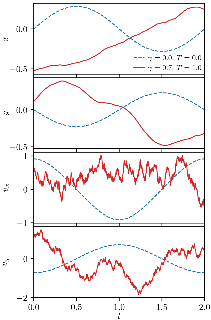
Figure 1: Phase space coordinates $(x,y,v_{x},v_{y})$ of two trajectories arbitrarily selected from the ensemble of TS trajectories on the NHIM at $T=0$ and $T=1.0$, respectively. The non-thermal trajectory ($T=0$, $\gamma=0$) is periodic with the driving frequency $\omega=\pi$ of the potential, as can be readily seen. The thermal trajectory ($T=1.0$, $\gamma=0.7$), in contrast, exhibits fluctuations characteristic of the stochastic driving, and it spreads out of sync with the periodic driving.

The effect of the Langevin dynamics on the trajectories of the system is illustrated in Fig. 1. The phase space coordinates of two arbitrary TS trajectories on the NHIM are shown. In the non-thermal case we can see that the trajectory follows a smooth path in phase space and it is periodic in sync with the deterministic driving. In contrast, the trajectory of the thermal system fluctuates significantly, especially in the velocities. The stochastic and aperiodic motion of the thermal trajectories presents a new challenge for our earlier methods on non-thermal systems Bardakcioglu et al. (2018); Feldmaier et al. (2019a, b); Tschöpe et al. (2020) addressed here.

II.2 Identification of the NHIM

The NHIM, barring any general definition and here only limited to a rank-1 saddle potential, is the set of all trajectories in phase space bound forever to the saddle region in both forward and backward in time directions. It is a manifold of co-dimension two in phase space. It is also associated with a pair of stable and unstable manifolds of co-dimension one, whose closures intersect at the NHIM. For our model chemical reaction [Eq. (4)], the position $(x,v_{x})^{\mathrm{NHIM}}(y,v_{y})$ of the NHIM can be parameterized as a function of the stable orthogonal modes $y$ and $v_{y}$ at a specific time $t$.

The motion of individual trajectories in a close neighborhood of the NHIM is stochastic for a thermal system as illustrated in Fig. 1. Nevertheless, the corresponding stable and unstable manifolds in Fig. 2(a) remain smooth, and generally so. Thus, even for a thermal system, the phase space in a local neighborhood looks similar to a non-thermal system, as also observed in Refs. Bardakcioglu et al. (2018); Feldmaier et al. (2019a, b); Tschöpe et al. (2020). Hence, the typical cross-like intersection of the stable and unstable manifolds is preserved and the position of the NHIM can be directly obtained from the intersection of the stable and the unstable manifolds. In a thermal system, however, the intersection $(x,v_{x})^{\mathrm{NHIM}}(y,v_{y})$ will not only depend on the specific choice of the orthogonal modes $(y,v_{y})$, but also on the parameters $\gamma$ and $T$. This finding is illustrated in Fig. 2(a) for the paradigmatic system used throughout this work.

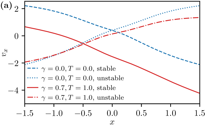
Figure 2: (a) Stable and unstable manifold at orthogonal modes $y=v_{y}=0$ for a non-thermal and thermal system with driving frequency $\omega=\pi$. The intersection of these manifolds mark the $x$ and $v_{x}$ coordinate of the NHIM for these orthogonal modes. Crosses such as these can be obtained for any orthogonal modes $(y,v_{y})$ and time $t$. Thus, one can express the reaction coordinates $(x,v_{x})^{\mathrm{NHIM}}(y,v_{y},t)$ of the NHIM as functions of initial time and orthogonal modes. (b) Sketch of the stable and unstable manifold. The arrowheads indicate the projected path trajectories take within the four separated regions. A quadrangle with a vertex in each of the four regions illustrates the binary contraction method, an iterative routine to find the NHIM at the intersection of the manifolds, see Sec. II.2.

The stable and unstable manifolds have the characteristic property that any trajectory near them is propagated towards or away from the NHIM, respectively. Only at the intersection of their closures—viz. the NHIM— trajectories are unstably bound to the saddle region. As the stable and unstable manifold are themselves invariant manifolds, they cannot be crossed by any trajectory of the system. This effectively separates the phase space in the close neighborhood of the NHIM into four distinct regions demarcated by these manifolds, see Fig. 2(b). For a chosen saddle region $x\in[x_{\mathrm{min}},x_{\mathrm{max}}]$ with appropriately chosen boundaries $x_{\mathrm{min}}$ and $x_{\mathrm{max}}$, the dynamics of trajectories is characteristic for any of these regions, as indicated with the black arrows in Fig. 2(b). In region (I), non-reactive trajectories originate from the reactant side $x<x_{\mathrm{min}}$ in the past and fall back to the reactant side in the future. The same is true for region (III) which contains all trajectories that originate from the product side $x>x_{\mathrm{max}}$ and also fall back to the product side. Regions (II) and (IV) hold the reactive trajectories from the reactant to the product side or, respectively, vice versa.

We use the binary contraction method (BCM) Bardakcioglu et al. (2018) to numerically find the NHIM at a given time $t$ for a given set $(y,v_{y})$ of orthogonal modes. The procedure of the BCM is initiated with a quadrangle having its four vertices (blue dots in Fig. 2(b)) in each of the four reactive and non-reactive regions in a close neighborhood of the NHIM. In successive steps, the midpoint between pairs of nearby points of the quadrangle is propagated to determine which region it belongs to and then replaces the corresponding point. The area of the quadrangle thus shrinks and its center converges to the intersection $(x,v_{x})^{\mathrm{NHIM}}(y,v_{y})$ of the manifold. The resulting $(y,v_{y})$ corresponds to the position $(x,v_{x})$ of the NHIM. This convergence is exponentially fast and, therefore, the BCM is very efficient in finding the NHIM for a given set of orthogonal modes. For the technical details of the BCM, we refer the reader to Ref. Bardakcioglu et al. (2018).

II.3 Trajectories on the NHIM

Due to the hyperbolic nature of the NHIM, trajectories on the NHIM are unstable. Small deviations from the NHIM will grow exponentially in time until the trajectory leaves its immediate vicinity. Thus any deviation in a point relative to the NHIM, no matter how small, will lead its subsequent propagation to fall off of it eventually. This presents a challenge to the propagation of trajectories on the NHIM using numerical simulations.

These numerical deviations can be suppressed through a machine-learning representation of the NHIM projecting them back onto the NHIM as has been done in Ref. Tschöpe et al. (2020). Here, we employ this approach leveraging the numerically accurate BCM presented in Ref. Bardakcioglu et al. (2018). Given the system and bath parameters, the reaction coordinate and corresponding velocity of the NHIM can be integrated in time as a function of the remaining orthogonal modes in the usual way. By subsequently projecting the trajectory back onto the NHIM it is effectively propagated in a system with reduced dimensions which is spanned by the orthogonal modes. The result is a trajectory that remains on the NHIM.

II.4 Decay rates of reactant population

The relative stability of the NHIM can be characterized through the instantaneous decay rates $k(y,v_{y},t)$ of the reactant population for the specific orthogonal modes $(y,v_{y})$ in its close neighborhood at each time $t$. These decay rates can be obtained directly by propagating ensembles of reactive trajectories but this can become cumbersome and numerically expensive. The local manifold analysis (LMA) was introduced in Ref. Feldmaier et al. (2019b) to overcome this problem by leveraging the linear dynamics near the NHIM.

Since the dynamics relative to the transition state is linear, it is possible to propagate trajectories using a linear map, the fundamental matrix $\boldsymbol{M}$, obtained via

$$\dot{\boldsymbol{M}}=\boldsymbol{J}(t)\boldsymbol{M}\,,$$ (5)

with the initial condition of $\boldsymbol{M}(t_{0})=\mathbf{1}$, and a Jacobian

$$\boldsymbol{J}(t)=\frac{\partial(\dot{\boldsymbol{x}},\dot{\boldsymbol{v}})}{\partial(\boldsymbol{x},\boldsymbol{v})}=\begin{pmatrix}0&0&1&0\\ 0&0&0&1\\ -\frac{\partial^{2}V}{\partial x^{2}}&-\frac{\partial^{2}V}{\partial x\partial y}&-\gamma&0\\ -\frac{\partial^{2}V}{\partial x\partial y}&-\frac{\partial^{2}V}{\partial y^{2}}&0&-\gamma\\ \end{pmatrix}\,$$ (6)

parameterized in time along a specific trajectory of the transition state. The stochastic force $\boldsymbol{\xi}(t)$ does not contribute to any component of the Jacobian in Eq. (6) as it is purely time-dependent. However, this does not mean that it is neglected in the Langevin dynamics. The Jacobian (6) describes the motion relative to a transition state whose trajectory is fluctuating under the influence of the stochastic force. That means that although the dynamics relative to the close vicinity of the transition state might not be fluctuating, the total dynamics still does. Using the linear dynamics near the transition state according to Eq. (5), we can extract the instantaneous motion of a particle ensemble near that state from the Jacobian.

The LMA models the presence of such a uniform particle ensemble in the close neighborhood of the NHIM. For the system of Eqs. (1) and (4) at specific orthogonal modes $(y,v_{y})$ and time $t$, we can obtain a local instantaneous decay rate

$$k(y,v_{y},t)=\frac{\Delta v^{\mathrm{u}}_{x}}{\Delta x^{\mathrm{u}}}(y,v_{y},t)-\frac{\Delta v^{\mathrm{s}}_{x}}{\Delta x^{\mathrm{s}}}(y,v_{y},t)\,,$$ (7)

where $\Delta v^{\mathrm{s,u}}_{x}/\Delta x^{\mathrm{s,u}}$ represents the slopes of the stable and unstable manifolds in the corresponding $(x,v_{x})$ cross section of the full phase space near the transition state. Determining these slopes, or rather the instantaneous decay rate as the difference of these slopes, is the main objective of the numerical implementation of the LMA. A derivation of the LMA can be found in Ref. Feldmaier et al. (2019b), and the additional corrections that would be necessary for more general cases can be found in the Supplementary Material of Ref. Feldmaier et al. (2020).

An average rate for the decay relative to trajectories on the NHIM is obtained by computing the time average of the instantaneous decay rates for a sufficiently long time to obtain convergence. For a trajectory that is initialized at time $t_{0}$ and position $(y_{0},{v_{y}}_{0})$ on the NHIM, and parameterized by the orthogonal modes $y(t)$ and $v_{y}(t)$, this average yields

$$\bar{k}(y_{0},{v_{y}}_{0},t_{0})=\lim_{\tau\rightarrow\infty}\frac{1}{\tau}\int_{t_{0}}^{t_{0}+\tau}k(y(t^{\prime}),v_{y}(t^{\prime}),t^{\prime})\,\mathrm{d}t^{\prime}\,.$$ (8)

In the special case of $T=0$, we find that the trajectories are periodic or quasi-periodic, and it suffices to integrate for the period or quasi-period. An alternative approach to obtain mean decay rates is provided by a Floquet analysis of said trajectory Feldmaier et al. (2019b); Craven et al. (2014)

$$\bar{k}(y_{0},{v_{y}}_{0},t_{0})=\lim_{\tau\rightarrow\infty}\frac{1}{\tau}\left(\ln{|m_{\mathrm{l}}(\tau)|}-\ln{|m_{\mathrm{s}}(\tau)|}\right)\,,$$ (9)

where $m_{\mathrm{l,s}}(t)$ are the eigenvalues of the fundamental matrix $\boldsymbol{M}$. It reduces to the monodromy matrix when the trajectory is periodic. Here, the subscripts l and s denote the eigenvalues with the largest and smallest absolute values, respectively Craven et al. (2014); Feldmaier et al. (2019b).

III Results and discussion

III.1 Stochastic motion of the NHIM under noise

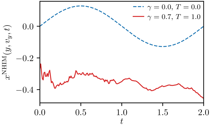
Figure 3: Position $x^{\mathrm{NHIM}}$ of the NHIM for fixed $y=v_{y}=0$ and $\omega=\pi$ as a function of time. Without the Langevin terms, the NHIM (dashed curve) oscillates periodically, as one would expect from the periodically driven saddle potential. With the Langevin terms, however, the NHIM (solid curve) moves stochastically. Compared to a trajectory on the NHIM for the same parameters, the reaction coordinates $x$ does not fluctuate as much as the NHIM in phase space, see Fig. 1.

The time-dependent NHIM and the associated decay rates in a driven chemical reaction are resolved here for the model system of Eq. (1). If the dissipative and stochastic terms are excluded, the result is a smooth oscillating motion with the same period as that of the oscillating potential Feldmaier et al. (2020). However, when the system is subject to the Langevin terms—viz. friction and thermal noise—the motion of the NHIM becomes stochastic as illustrated in Fig. 3. Here, the expected behavior in the time-dependence of $x^{\mathrm{NHIM}}$ for a specific set of coordinates $(y,v_{y})$ in the dynamics without and with the Langevin terms is apparent. The latter case now exhibits stochastic fluctuations in both position (as shown) and momentum (as not shown) space. They are in response to the combination of the collective stochastic thermal driving and the periodic driving terms. Such fluctuations were not seen in the position space of the TS trajectories shown in Fig. 1 because in this relatively weak friction regime, the high-frequency fluctuations are very small. However, in Fig. 3, the NHIM does exhibit short-time fluctuations in the position space as a manifestation of the overall phase space motion. Nevertheless, the DS is recrossing-free as it incorporates the noise.

III.2 Dissipative dynamics on the NHIM

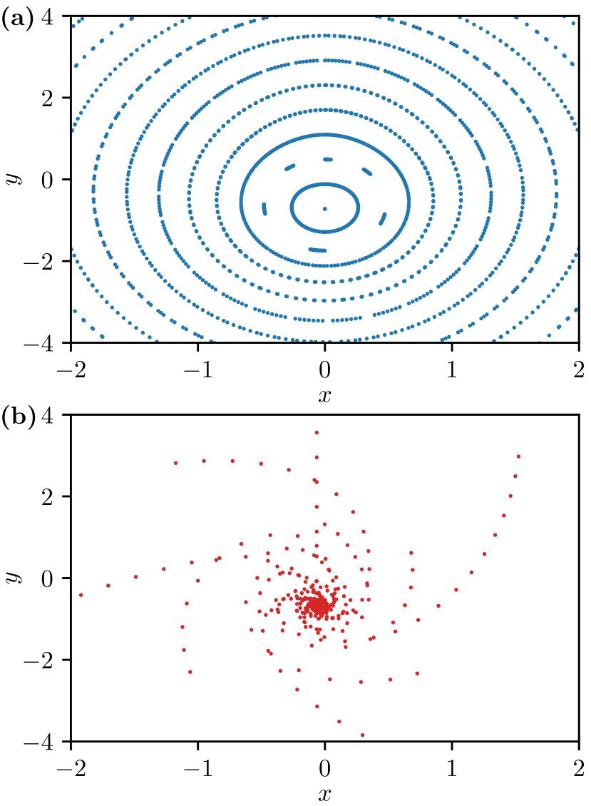
Figure 4: The PSOSs of the system defined by Eqs. (1) and (4) for varying friction at temperature $T=0$ and saddle frequency $\omega=\pi$. The non-thermal system with friction $\gamma=0$ and the thermal system with $\gamma=0.2$ are shown in panels (a) and (b), respectively. In panel (a), the regularity of the system is demonstrated by the elliptic fixed point at the center and the surrounding tori. In panel (b), for trajectories with similar initial conditions as in (a), the stroboscopic dynamics on the NHIM collapses to a fixed point in the dissipative case.

Although we have seen that the dynamics of the system in the general case of Eq. (1) for the potential in (4) is not periodic, it is nevertheless instructive to examine the stroboscopic Poincaré surface of section (PSOS) of its trajectories. Similar to the approach used in Refs. Feldmaier et al. (2019b); Reiff et al. , we record the position of trajectories in the $(y,v_{y})$ section in phase space at time steps equal to the period of the driving. As we start with a point on the NHIM, it necessarily must stay on the NHIM. Thus, the coordinates in the PSOS, as seen e. g. in Fig. 4, remain projected onto the NHIM.

The PSOSs of Fig. 4 show the contrast in the dynamics upon the introduction of friction. In the upper panel, the dynamics on the NHIM is regular. It gives rise to the expected stable concentric tori and an elliptic fixed point. In the bottom panel, as a result of the friction, the would-be tori now spiral towards a fixed point in the stroboscopic projection. This fixed point refers to a time-periodic trajectory in phase space, which acts as an attractor for particles on the NHIM.

III.3 Thermal decay rates

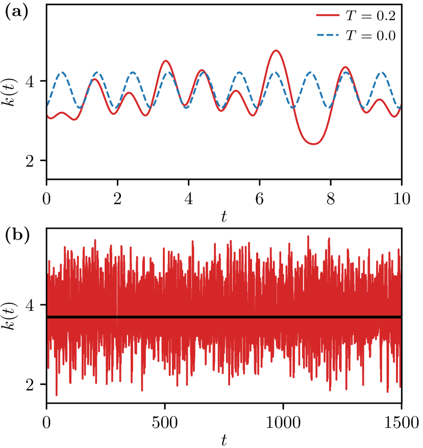
Figure 5: (a) Comparison of instantaneous decay rates of the equilibrium trajectory on the NHIM as defined in Sec. III.3 for friction $\gamma=0.2$ and temperatures $T=0.2$ and $0$, respectively. The driving frequency in both cases is $\omega=\pi$. The instantaneous rate of the thermal complex roughly follows the oscillations of the non-thermal trajectory but exhibits fluctuations to a certain degree. (b) Instantaneous rate of the thermal activated complex in over a longer time interval. Stochastic fluctuations of the rate become more evident over hundreds of saddle oscillation periods. The dashed line highlights the time-average of the rate.

The collapse of the NHIM to a single periodic trajectory in dissipative regimes with temperature $T=0$ observed in Sec. III.2 can be used to our advantage for temperatures above zero. Even when noise is in play, the fluctuating trajectories on the NHIM will approach a single fluctuating trajectory over long times, which we will refer to as the equilibrium trajectory on the NHIM. It can be determined numerically by propagating an arbitrary point on the NHIM for a sufficiently long time until the equilibrium is reached. The initial build-up is discarded when calculating rates. In the infinite time limit, use of the equilibrium trajectory to obtain the average decay rate $\bar{k}$ eliminates its dependence on the initial conditions $(y_{0},{v_{y}}_{0},t_{0})$ in Eqs. (8) and (9). That is, all contributions to the average decay rate that would depend on the initial conditions are dwarfed by the contributions of the equilibrium trajectory.

Assuming that the long-term behavior is independent of the initial time $t_{0}$, the equilibrium trajectory can be used to construct the expected value $\left<k\right>(T,\gamma)$ of the reactant decay rate as a function of the temperature $T$ and friction $\gamma$

$$\left<k\right>(T,\gamma)=\bar{k}(y_{0},{v_{y}}_{0},t_{0};T,\gamma)\,,$$ (10)

which, due to the fact that the initial conditions will be forgotten by the dynamics over time, is the same for any set of initial conditions $(y_{0},{v_{y}}_{0},t_{0})$.

III.3.1 Instantaneous decay rates

The influence of the noise on the average decay rate is revealed by the time evolution of the instantaneous decay rate. The rates shown in Fig. 5(a) are plotted over five saddle oscillations. Despite the stochastic nature of the NHIM at fixed orthogonal modes $(y,v_{y})$, we find that the instantaneous rate of the thermal trajectory on the NHIM is smooth and still roughly follows the regular oscillation we find for zero temperature. This can be attributed to the fact that the trajectories, as integrated values over a noisy acceleration, have a smooth time evolution. Despite the instant decay in the time correlation of the stochastic force in the fluctuation-dissipation relation [Eq. (3)], these trajectories have a finite memory of their previous positions Zwanzig (1961). However, over sufficiently long time scales, it is possible to obtain a time evolution of the instantaneous reactant decay rate that resembles an uncorrelated fluctuation, as can be seen in Fig. 5(b).

III.3.2 Temperature dependence of average decay rates

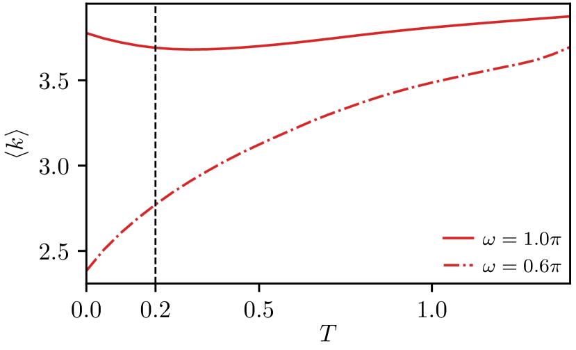
Figure 6: Temperature dependent time-average of the instantaneous decay rate for the activated complex of the model system at two different driving frequencies, $\omega=0.6\pi$ and $1.0\pi$. The dotted vertical line highlights the average rates at $T=0.2$ corresponding to the data in Figs. 5 and 7.

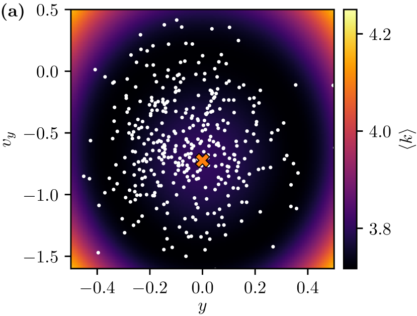
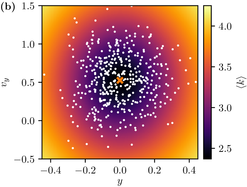
Figure 7: Stroboscopic projections of a typical trajectory on the NHIM for each of the saddle driving frequencies, (a) $\omega=\pi$ and (b) $\omega=0.6\pi$, in the dissipated thermal case, $\gamma=0.2$ and $T=0.2$, are shown as white filled circles. Refer to Fig. 6 for the corresponding average rates where the vertical dashed line crosses the curves. The color maps show the time-averaged decay rates $\left<k\right>$ of a non-thermal activated complex on the NHIM for the initial conditions $(y,v_{y})$ at time $t_{0}=0$. For reference, the fixed points of the stroboscopic maps in the non-thermal case are indicated by a cross.

The averaged rate has to be determined over several hundreds—sometimes even a few thousand—saddle oscillations to obtain a statistically-sound converged average. This is as a consequence of the need to achieve the limiting equilibrium trajectory as observed in Sec. III.3.1. The resulting temperature dependence of the averaged decay rate for two sets of parameters is shown in Fig. 6. These parameters were chosen, as they give rise to two very different regimes in the shape of the rate from concave to convex. With a driving frequency of $\omega=0.6\pi$, we obtain a rate that is monotonically rising, as temperature rises. However, at a driving frequency of $\omega=\pi$, we obtain a rate that at first decreases, before it increases with rising temperature.

The change in behavior of the rate curves may seem counter-intuitive at first. One might expect that a higher temperature—i. e., a higher average energy—would cause the reaction to surmount an energy barrier at a higher rate. This expectation is not contradicted by the present results. The decay rate computed here is the decay rate of the reactant population close to the transition state, i. e., the rate of reaction after the reactant has already surmounted the energy barrier. Such a rate does not include the increased population of activated reactants that would arise from a higher temperature and consequently does not have to increase accordingly.

We find that strong noise causes the activated complex to fluctuate strongly near the NHIM as seen in Fig. 7. When comparing these coordinate fluctuations with the phase space resolved decay rates of the non-thermal system according to Fig. 7 or additional examples in the Supplemental Material p (22), we can also see how a thermal activated complex explores several transition states of the non-thermal system. This further suggests that the decay of the thermal activated complex into reactants or products is related to the distribution of the explored, non-thermal transition states. This interpretation is consistent with the observation made in Sec. II.4 that noise only affects the average decay rate by the trajectory that is used to obtain it. Even though this analogy is not formally exact since the Jacobian $\boldsymbol{J}$ according to Eq. (6) contains the friction coefficient $\gamma$—which is not zero in the thermal case—the conjectured interpretation appears to hold for the low-temperature thermal case discussed in Figs. 6 and 7.

A heuristic argument in support of the conjecture is as follows. As temperature rises, the activated complex deviates further from the corresponding periodic trajectory at $T=0$. This in turn causes the activated complex to explore transition states that are further from said trajectory. Moreover, the distribution of explored transition states expands into a region with shrinking decay rates as temperature rises. The equilibrium trajectory now resides in a local maximum of decay rates, as is the case for $\omega=0.6\pi$, and hence the decay of the activated complex decreases with rising temperature.

IV Summary and conclusion

We have characterized the geometric structure of a model chemical reaction, thereby taking into account both external driving and noise and friction described by the Langevin terms. We have shown that the temperature dependence of the activated complex decay in this thermal system is linked to the distribution of the phase space resolved decay rates on the NHIM in the non-dissipative case. The decay rate of the activated complex depends on the external driving and the temperature, and these dependencies can be used to control the reaction.

In this paper we have investigated the thermal decay rates of trajectories very close to the NHIM based on equilibrium trajectories located exactly on the NHIM. In future work it will be necessary to also study trajectories out of the NHIM. An important question is whether one can define a thermal equilibrium or at least a stationary distribution on the DS in these nonequilibrium systems with which one can obtain the reaction rate.

Recently, we have investigated the influence of external driving on decays in the geometry of the LiCN isomerization without considering noise and friction Feldmaier et al. (2020). Meanwhile, the dissipation arising from an argon bath on that reaction was seen to be representable by the Langevin terms Junginger et al. (2016b). Thus, the methods presented here open up the possibility of considering the thermal effects in a driven LiCN isomerization reaction and other chemical reactions of interest.

V Acknowledgments

The German portion of this collaborative work was supported by Deutsche Forschungsgemeinschaft (DFG) through Grant No. MA1639/14-1. RH’s contribution to this work was supported by the National Science Foundation (NSF) through Grant No. CHE-1700749. M.F. is grateful for support from the Landesgraduiertenförderung of the Land Baden-Württemberg. This collaboration has also benefited from support by the European Union’s Horizon 2020 Research and Innovation Program under the Marie Skłodowska-Curie Grant Agreement No. 734557.

References

- Eyring (1935) H. Eyring, J. Chem. Phys. 3, 107 (1935).
- Wigner (1937) E. P. Wigner, J. Chem. Phys. 5, 720 (1937).
- Pitzer et al. (1962) K. S. Pitzer, F. T. Smith, and H. Eyring, The Transition State, Special Publ. (Chemical Society, London, 1962) p. 53.
- Pechukas (1981) P. Pechukas, Annu. Rev. Phys. Chem. 32, 159 (1981).
- Garrett and Truhlar (1979) B. C. Garrett and D. G. Truhlar, J. Phys. Chem. 83, 1052 (1979).
- Truhlar et al. (1985) D. G. Truhlar, A. D. Issacson, and B. C. Garrett, “Theory of chemical reaction dynamics,” (CRC Press, Boca Raton, FL, 1985) pp. 65–137.
- Natanson et al. (1991) G. A. Natanson, B. C. Garrett, T. N. Truong, T. Joseph, and D. G. Truhlar, J. Chem. Phys. 94, 7875 (1991).
- Truhlar et al. (1996) D. G. Truhlar, B. C. Garrett, and S. J. Klippenstein, J. Phys. Chem. 100, 12771 (1996).
- Truhlar and Garrett (2000) D. G. Truhlar and B. C. Garrett, J. Phys. Chem. B 104, 1069 (2000).
- Komatsuzaki and Berry (2001) T. Komatsuzaki and R. S. Berry, Proc. Natl. Acad. Sci. U.S.A. 98, 7666 (2001).
- Waalkens et al. (2008) H. Waalkens, R. Schubert, and S. Wiggins, Nonlinearity 21, R1 (2008).
- Bartsch et al. (2008) T. Bartsch, J. M. Moix, R. Hernandez, S. Kawai, and T. Uzer, Adv. Chem. Phys. 140, 191 (2008).
- Kawai and Komatsuzaki (2010) S. Kawai and T. Komatsuzaki, Phys. Rev. Lett. 105, 048304 (2010).
- Hernandez et al. (2010) R. Hernandez, T. Bartsch, and T. Uzer, Chem. Phys. 370, 270 (2010).
- Sharia and Henkelman (2016) O. Sharia and G. Henkelman, New J. Phys. 18, 013023 (2016).
- Keck (1967) J. C. Keck, Adv. Chem. Phys. 13, 85 (1967).
- Mullen et al. (2014) R. G. Mullen, J.-E. Shea, and B. Peters, J. Chem. Phys. 140, 041104 (2014).
- Miller (1998) W. H. Miller, J. Phys. Chem. A 102, 793 (1998).
- Feldmaier et al. (2017) M. Feldmaier, A. Junginger, J. Main, G. Wunner, and R. Hernandez, Chem. Phys. Lett. 687, 194 (2017).
- Feldmaier et al. (2019a) M. Feldmaier, P. Schraft, R. Bardakcioglu, J. Reiff, M. Lober, M. Tschöpe, A. Junginger, J. Main, T. Bartsch, and R. Hernandez, J. Phys. Chem. B 123, 2070 (2019a).
- Pollak (1990) E. Pollak, J. Chem. Phys. 93, 1116 (1990).
- Uzer et al. (2002) T. Uzer, C. Jaffé, J. Palacián, P. Yanguas, and S. Wiggins, Nonlinearity 15, 957 (2002).
- Bartsch et al. (2005a) T. Bartsch, R. Hernandez, and T. Uzer, Phys. Rev. Lett. 95, 058301 (2005a).
- Wiggins (2016) S. Wiggins, Regul. Chaotic Dyn. 21, 621 (2016).
- Junginger et al. (2016a) A. Junginger, G. T. Craven, T. Bartsch, F. Revuelta, F. Borondo, R. M. Benito, and R. Hernandez, Phys. Chem. Chem. Phys. 18, 30270 (2016a).
- Craven et al. (2017) G. T. Craven, A. Junginger, and R. Hernandez, Phys. Rev. E 96, 022222 (2017).
- Brown (1828) R. Brown, Philos. Mag. 4, 161 (1828), ibid. 6, 161 (1829).
- Kramers (1940) H. A. Kramers, Physica (Utrecht) 7, 284 (1940).
- Hänggi et al. (1990) P. Hänggi, P. Talkner, and M. Borkovec, Rev. Mod. Phys. 62, 251 (1990), and references therein.
- Mel’nikov and Meshkov (1986) V. I. Mel’nikov and S. V. Meshkov, J. Chem. Phys. 85, 1018 (1986).
- Pollak et al. (1989) E. Pollak, H. Grabert, and P. Hänggi, J. Chem. Phys. 91, 4073 (1989).
- García-Müller et al. (2008) P. L. García-Müller, F. Borondo, R. Hernandez, and R. M. Benito, Phys. Rev. Lett. 101, 178302 (2008).
- García-Müller et al. (2012) P. L. García-Müller, R. Hernandez, R. M. Benito, and F. Borondo, J. Chem. Phys. 137, 204301 (2012).
- Junginger et al. (2016b) A. Junginger, P. L. García-Müller, F. Borondo, R. M. Benito, and R. Hernandez, J. Chem. Phys. 144, 024104 (2016b).
- Lichtenberg and Liebermann (1982) A. J. Lichtenberg and M. A. Liebermann, Regular and Stochastic Motion (Springer, New York, 1982).
- Hernandez and Miller (1993) R. Hernandez and W. H. Miller, Chem. Phys. Lett. 214, 129 (1993).
- Hernandez (1993) R. Hernandez, Ph.D. thesis, University of California, Berkeley, CA (1993).
- Ott (2002) E. Ott, Chaos in dynamical systems, second edition ed. (Cambridge University Press, Cambridge, 2002).
- Wiggins (2013) S. Wiggins, Normally hyperbolic invariant manifolds in dynamical systems, Vol. 105 (Springer Science & Business Media, 2013).
- Feldmaier et al. (2019b) M. Feldmaier, R. Bardakcioglu, J. Reiff, J. Main, and R. Hernandez, J. Chem. Phys. 151, 244108 (2019b).
- Langer (1969) J. S. Langer, Ann. Phys. (N.Y., NY, U.S.) 54, 258 (1969).
- Eli Pollak (1995) E. Eli Pollak, J. Chem. Phys. 103, 973 (1995).
- Farkas (1927) L. Farkas, Z. Phys. Chem. (Leipzig) 125, 226 (1927).
- Pollak and Talkner (2005) E. Pollak and P. Talkner, Chaos 15, 026116 (2005).
- Tschöpe et al. (2020) M. Tschöpe, M. Feldmaier, J. Main, and R. Hernandez, Phys. Rev. E 101, 022219 (2020).
- Bartsch et al. (2005b) T. Bartsch, T. Uzer, and R. Hernandez, J. Chem. Phys. 123, 204102 (2005b).
- Bartsch et al. (2012) T. Bartsch, F. Revuelta, R. M. Benito, and F. Borondo, J. Chem. Phys. 136, 224510 (2012).
- (48) J. Reiff, R. Bardakcioglu, M. Feldmaier, J. Main, and R. Hernandez, “Enhancing and controlling rates in model chemical reactions through external driving,” in preparation.
- Bardakcioglu et al. (2018) R. Bardakcioglu, A. Junginger, M. Feldmaier, J. Main, and R. Hernandez, Phys. Rev. E 98, 032204 (2018).
- Kubo (1966) R. Kubo, Rep. Prog. Phys. 29, 255 (1966).
- Keizer (1976) J. Keizer, J. Chem. Phys. 64, 1679 (1976).
- Hernandez and Somer (1999) R. Hernandez and F. L. Somer, J. Phys. Chem. B 103, 1064 (1999).
- Schraft et al. (2018) P. Schraft, A. Junginger, M. Feldmaier, R. Bardakcioglu, J. Main, G. Wunner, and R. Hernandez, Phys. Rev. E 97, 042309 (2018).
- Kuchelmeister et al. (2020) M. Kuchelmeister, J. Reiff, J. Main, and R. Hernandez, Regul. Chaotic Dyn. 25, 496–507 (2020).
- Feldmaier et al. (2020) M. Feldmaier, J. Reiff, R. M. Benito, F. Borondo, J. Main, and R. Hernandez, J. Chem. Phys. 153, 084115 (2020).
- Craven et al. (2014) G. T. Craven, T. Bartsch, and R. Hernandez, J. Chem. Phys. 141, 041106 (2014).
- Zwanzig (1961) R. Zwanzig, Phys. Rev. 124, 983 (1961).
- p (22) See Supplemental Material at https://link.aps.org/supplemental/10.1103/PhysRevE.102.062204 for average decay rates at various temperatures.