A Survey on Advancing the DBMS Query Optimizer: Cardinality Estimation, Cost Model, and Plan Enumeration

Abstract.

Query optimizer is at the heart of the database systems. Cost-based optimizer studied in this paper is adopted in almost all current database systems. A cost-based optimizer introduces a plan enumeration algorithm to find a (sub)plan, and then uses a cost model to obtain the cost of that plan, and selects the plan with the lowest cost. In the cost model, cardinality, the number of tuples through an operator, plays a crucial role. Due to the inaccuracy in cardinality estimation, errors in cost model, and the huge plan space, the optimizer cannot find the optimal execution plan for a complex query in a reasonable time. In this paper, we first deeply study the causes behind the limitations above. Next, we review the techniques used to improve the quality of the three key components in the cost-based optimizer, cardinality estimation, cost model, and plan enumeration. We also provide our insights on the future directions for each of the above aspects.

1. Introduction

Query optimizer is at the heart of relational database management systems (RDBMSes) and some big data process engines, e.g. SCOPE (Chaiken et al., 2008). Given a query written in a declarative language (e.g., SQL), the optimizer finds the most efficient execution plan (also called physical plan) and feeds it to the executor. Thus, most of the time, the users only think over how to transform their requirements to a valid query without the need to analyze how to run the query efficiently. Almost all systems adopt a cost-based optimizer based on the architecture of System R (Selinger et al., 1979) or Volcano/Cascades (Graefe and McKenna, 1993; Graefe, 1995).

Figure 1 illustrates the three most important components in a cost-based optimizer: cardinality estimation (CE), cost model (CM), and plan enumeration (PE). CE uses statistics of data and some assumptions about data distribution, column correlation, and join relationship to get the number of tuples generated by an intermediate operator, which is also crucial for other search problems, e.g., (Yang et al., 2019b, c). CM can be regarded as a complex function that maps the current state of database and estimated cardinalities to the cost of executing a (sub)plan. PE is an algorithm to explore the space of semantically equivalent join orders and find the optimal orders with minimal cost. There are two principal approaches to find an optimal join order: bottom-up join enumeration via dynamic programming and top-down join enumeration through memorization.

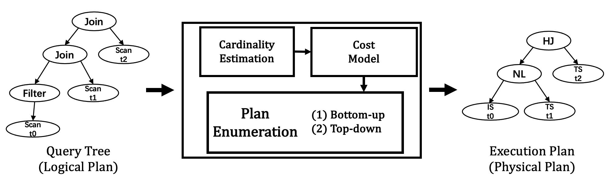
Figure 1. Query optimizer architecture. IS, HJ, NL, and TS refer to index scan, hash join, nestloop join, and table scan.

Cost-based optimizer.

Theoretically, provided that the estimated cardinality and cost are accurate, and plan enumeration component can efficiently walk through the huge search space, this architecture can obtain the optimal execution plan in a reasonable time. However, it fails in reality. Despite decades of work, cost-based query optimizers still make mistakes on “difficult” queries due to the error in CE, the difficulty in building an accurate CM, and the pain in finding the optimal join orders (PE) for complex queries. The details are presented in Section 2, i.e., why the existing optimizer is still far from satisfaction.

There are lots of research studies proposed to improve the capability of the optimizer. In this paper, we present a survey on them. Specifically, we review the publications which are proposed to improve the capabilities of the three key components in the optimizer, i.e., CE, CM, PE.

This paper makes the following contributions:

1. We summarize the reasons why the CE, CM, and PE do not perform well (Section 2).

2. We review the studies proposed to estimate cardinality more accurately. According to the techniques used, we categorize them into synopsis-based methods, sampling-based methods, and learning-based methods (Section 3).

3. We review the work on improving the cost model. We classify them into three groups: improvement of the existing cost model, cost model alternatives, and performance prediction for a single query (Section 4).

4. We review the techniques used in plan enumeration and study the non-learning methods used to handle large queries. Besides, we review recent proposed methods, which adopt reinforcement learning to select the join order (Section 5).

5. In Sections 3-5, we present our insights on the future directions respectively.

There are two related surveys. In 1998, Chaudhuri (1998) reviews the work with non-learning methods on query optimizer. In the last two decades, many methods are proposed to improve the capability of the optimizer. It is necessary to review the new work. Recently, Zhou et al. (2020) investigate how AI is introduced in the different parts of DBMS, such as monitoring, tuning, optimizer. In this paper, we focus on the query optimizer and give a comprehensive survey on the three key components of the optimizer. We summarize the learning-based and non-learning methods at the same time, review these work in details, and present possible future directions for each of them.

2. Why Key Components In Optimizer Are Still Not Accurate?

In this section, we summarize the reasons why the cardinality estimation, cost model, and plan enumeration do not perform well respectively. The studies reviewed in this paper try to improve the quality of the optimizer by handling these shortages.

2.1. Cardinality Estimation

Cardinality estimation is the ability to estimate the tuples generated by an operator and is used in the cost model to calculate the cost of that operator. Lohman (2014) points out that the cost model can introduce errors of at most 30%, while the cardinality estimation can easily introduce errors of many orders of magnitude. Leis et al. (2015) experimentally revisit the components, CE, CM, and PE in the classical optimizers with complex workloads. They focus on the quality of the physical plan on multi-join queries and get the same conclusion with Lohman.

The errors in cardinality estimation are mainly introduced in three cases:

1. Error in single table with predications. Database systems usually take histograms as the approximate distribution of data. Histograms are smaller than the original data. Thus, it cannot represent the true distribution entirely and some assumptions (e.g. uniformity on a single attribute, independence assumption among different attributes) are proposed. When those assumptions are not hold, estimation errors occur, leading to sub-optimal plans. The correlation among attributes in a table is not unusual. Multi-histograms have been proposed. However, it suffers from a large storage size.

2. Error in multi-join queries. Correlations possibly exist in columns from different tables. However, there is no efficient way to get synopses between two or more tables. Inclusion principle has been introduced for this case. The cardinality of a join operator is calculated using the inclusion principle with cardinalities of its children. It has large errors when the assumption is not held. Besides, for a complex query with multiple tables, the estimation errors can propagate and amplify from the leaves to root of the plan. The optimizers of commercial and open-source database systems still struggle in cardinality estimation for mult-join queries (Leis et al., 2015).

3. Error in user defined function. Most of database systems support the user-defined function (UDF). When a UDF exists in the condition, there is no general method to estimate how many tuples satisfying it (Chaudhuri, 1998).

2.2. Cost Model

Cost-based optimizers use a cost model to generate the estimate of cost for a (sub)query. The cost of (sub)plan is the sum of costs of all operators in it.

The cost of an operator depends on the hardware where the database is deployed, the operator’s implementation, the number of tuples processed by the operator, and the current database state (e.g., data in the buffer, concurrent queries) (Manegold et al., 2002). Thus, a large number of magic numbers should be determined when combining all factors, and errors in cardinality estimation also affect the quality of the cost model. Furthermore, when the cost-based optimizer is deployed in a distributed or parallel database, the cloud environment, or the cross-platform query engines, the complexity of cost model is increasing dramatically. Moreover, even with the true cardinality, the cost estimation of a query is not linear to the running time, which may lead to a suboptimal execution plan (Kaoudi et al., 2020; Siddiqui et al., 2020).

2.3. Plan Enumeration

Plan enumeration algorithm is used to find the optimal join order from the space of semantically equivalent join orders such that the query cost is minimized. It has been proven to be an NP-hard problem (Ibaraki and Kameda, 1984). Exhaustive query plan enumeration is a prohibitive task for large databases with multi-join queries. Thus, it is crucial to explore the right search space which should consist of the optimal join orders or approximately optimal join orders and design an efficient enumeration algorithm. The join trees in the search space could be zig-zag trees, left-deep trees, right-deep trees, and bushy trees or the subset of them. Different systems consider different forms of join tree. There are three enumeration algorithms in traditional database systems: (1) bottom up join enumeration via dynamic programming (DP) (e.g., System R (Selinger et al., 1979)), (2) top-down join enumeration through memorization (e.g., Volcano/Cascades (Graefe and McKenna, 1993; Graefe, 1995)), and (3) randomized algorithms (e.g., genetic algorithm in PostgreSQL (Database, 2020) with numerous tables joining).

Plan enumeration suffers from three limitations: (1) the errors in cardinality estimation and cost model, (2) the rules used to prune the search space, and (3) dealing with the queries with large number of tables. When a query touches a large number of tables, optimizers have to sacrifice optimality and employ heuristics to keep optimization time reasonable, like genetic algorithm in PostgreSQL, greedy method in DB2, which usually generates poor plans.

We should notice the errors in cardinality will propagate to the cost model and lead to suboptimal join order. Eliminating or reducing the errors in cardinality is the first step to build a capable optimizer as Lohman (Lohman, 2014) says “The root of all evil, the Achilles Heel of query optimization, is the estimation of the size of intermediate results, known as cardinalities”.

In the following three sections, we summarize the research efforts made to handle limitations in CE, CM, and PE, i.e, how to make the query optimizer good.

3. Cardinality Estimation

At present, there are three major strategies for cardinality estimation as shown in Figure 2. We only list some representative work for each category. Every method tries to approximate the distribution of data well with less storage. Some proposed methods combine different techniques, e.g., (Tzoumas et al., 2011, 2013).

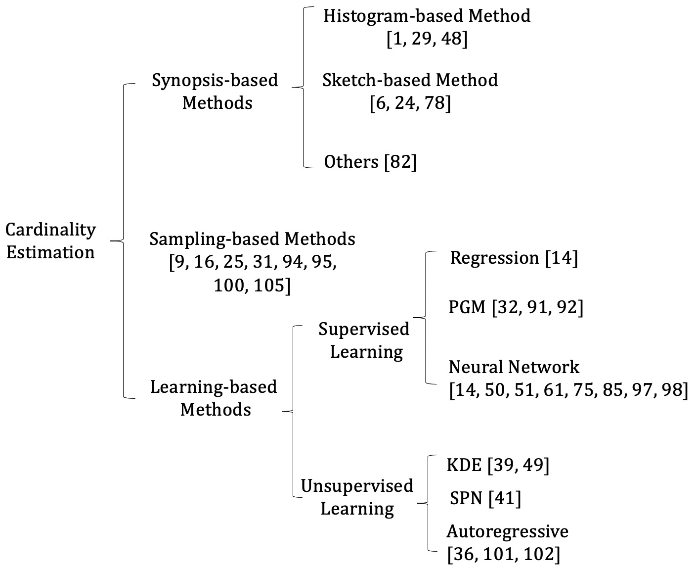
Figure 2. A classification of cardinality estimation methods

Cardinality estimation methods

3.1. Synopsis-based methods

Synopsis-based methods introduce new data structures to record the statistics information. Histogram and sketch are the widely adopted forms. A survey on synopses has been proposed in 2012 (Cormode et al., 2012), which focuses on distinguishing aspects of synopses that are pertinent to Approximate Query Processing (AQP).

3.1.1. Histogram

There are two histogram types: 1-dimensional and d-dimensional histograms, where $d\geq 2$. d-dimensional histograms can capture the correlation between different attributes.

A 1-dimensional histogram on attribute a is constructed by partitioning the sorted tuples into $B$ ($\geq 1$) mutually disjoint subsets, called buckets and approximates the frequencies and values in each bucket in some common fashion, e.g., uniform distribution and continuous values. A d-dimensional histogram on an attribute group A is constructed by partitioning the joint data distribution of A. Because there is no order between different attributes, the partition rule needs to be more intricate. In 2003, Ioannidis (2003) present a comprehensive survey on histograms following the classification method in (Poosala et al., 1996). Gunopulos et al. (2005) also propose a survey in 2003, which focuses on the work used to estimate the selectivity over multiple attributes. They summarize the multi-dimensional histograms and kernel density estimators. After 2003, the work in histograms can be divided into three categories: (1) fast algorithm for histogram construction (Guha et al., 2006; Halim et al., 2009, 2010; Indyk et al., 2012; Acharya et al., 2015); (2) new partition methods to divide the data into different buckets to achieve better accuracy (Eavis and Lopez, 2007; To et al., 2013; Lin et al., 2015); (3) histogram construction based on query feedback (Lim et al., 2003; Srivastava et al., 2006; Kaushik and Suciu, 2009). Query feedback methods are also summarized in (Cormode et al., 2012) (Section 3.5.1.2) and readers can refer to it for details.

Guha et al. (2006) analyze the previous algorithm, VODP (Jagadish et al., 1998) and, find some calculations on the minimal sum-of-squared-errors (SSE) can be reduced. They design an efficient algorithm AHistL-$\Delta$ with time complexity $O(n+B^{3}(\lg n+\epsilon^{-2}))$ while VODP takes $O(n^{2}B)$, where $n$ is the domain size, $B$ is the number of buckets, and $\epsilon$ is a precision parameter. Halim et al. (2009, 2010) propose GDY, a fast histogram construction algorithm based on greedy local search. GDY generates good sample boundaries, which then are used to construct $B$ final partitions optimally using VODP. This study compares GDY variants with AHistL-$\Delta$ (Guha et al., 2006) in minimizing the total errors of all the buckets and shows its superiority in resolving the efficiency-quality trade-off. Instead of scanning the whole dataset (Guha et al., 2006), Indyk et al. (2012) design a greedy algorithm to construct the histogram on the random samples from dataset with time complexity $O((B^{5}/\epsilon^{8})\log^{2}n)$ and sample complexity $O((B/\epsilon)^{2}\log n)$. Acharya et al. (2015) study the same problem with (Indyk et al., 2012) and propose a merging algorithm with time complexity $O(1/\epsilon^{2})$. Methods in (Guha et al., 2006; Indyk et al., 2012; Acharya et al., 2015) can be extended to approximate distributions by piecewise polynomials.

Considering the tree-based indexes divide the data into different segments (nodes), which is quite similar with buckets in the histogram, Eavis and Lopez (2007) build the multi-dimensional histogram based on R-tree. They first build a native R-tree histogram on the Hilbert sort of data, and then, propose a sliding window algorithm to enhance the naive histogram under a new proposed metric, which seeks to minimize the dead space between bucket points. Lin et al. (2015) design a two-level histogram for one attribute, which is quite similar to the idea of the B-tree index. The first level is used to locate which leaf histograms to be used, and the leaf histograms store the statistics information. To et al. (2013) construct a histogram based on the principle of minimizing the entropy reduction of the histogram. They design two different histograms for the equality queries and an incremental algorithm to construct the histogram. However, it only considers the one-dimensional histogram and does not handle range queries well.

3.1.2. Sketch

Sketch models a column as a vector or matrix to calculate the distinct count (e.g., HyperLogLog (Flajolet et al., 2007)) or frequency of tuples (e.g., Count Min (Cormode and Muthukrishnan, 2004)) on a value. Rusu and Dobra (2008) summarize how to use different sketches to estimate the join size. This work considers the case of two tables (or data streams) without filters. The basic idea of them is: (1) building the sketch (a vector or matrix) on the join attribute, while ignoring all the other attributes, (2) estimating the join size based on the multiplication of the vectors or matrices. These methods only support the equi-join and join on single column. As shown in (Vengerov et al., 2015), a possible method introducing one filter in sketch is to build an imaginary table which only consists of the join value of tuples which satisfy the filter. However, this makes the estimation drastically worse. Skimmed sketch (Ganguly et al., 2004) is based on the idea of bifocal sampling (Ganguly et al., 1996) to estimate the join size. However, it requires knowing frequencies of the most frequent join attribute values. Recent work (Cai et al., 2019) on join size estimation introduces the sketch to record the degree of a value.

3.1.3. Other Techniques

TuG (Spiegel and Polyzotis, 2006) is a graph-based synopsis. The node of TuG represents a set of tuples from the same table or a set of values for the same attribute. The edge represents the join relationship between different tables or between attributes and values. The authors adopt a three-step algorithm to construct TuG and introduce the histogram to summarize the value distribution in a node. When a new query comes, the selectivity is estimated by traversing TuG. The construction process is quite time-consuming and cannot be used in a large dataset. Without the relationship between different tables, TuG cannot be built.

3.2. Sampling-based Methods

Synopsis-based methods are quite difficult to capture the correlation between different tables. Some researchers try to use a specific sampling strategy to collect a set of samples (tuples) from tables, and then run the (sub)query over samples to estimate the cardinality. As long as the distribution of the obtained samples is close to the original data, the cardinality estimation is believable. Thus, lots of work have been proposed to design a good sampling approach, from independent sampling to correlated sampling technique. Sampling-based methods also are summarized in (Cormode et al., 2012). After 2011, there are numerous studies that utilize the sampling techniques. Different with (Cormode et al., 2012), we mainly summarize the new work. Moreover, we review the work according to their publishing time and present the relationship between them, i.e., which shortages of the previous work the later work tries to overcome.

In 1993, Haas et al. (1993) analyze the six different fixed-step (a pre-defined sample size) sampling methods for the equi-join queries. They conclude that if there are some indexes built on join keys, page-level sampling combining the index is the best way. Otherwise, the page-level cross-product sampling is the most efficient way. Then, the authors extend the fixed-step methods to fixed-precision procedures.

Ganguly et al. (1996) introduce bifocal sampling to estimate the size of an equi-join. They classify values of the join attribute in each relation into two groups, sparse (s) and dense (d) based on their frequencies. Thus, the join type between tuples can be s-s, s-d, d-s, and d-d. The authors first adopt t_cross sampling (Haas et al., 1993) to estimate the join size of d-d , then adopt t_index to estimate the join size of the remaining cases, and finally add all the estimation as the join size estimation. However, it needs an extra pass to determine the frequencies of different values and needs indexes to estimate the join size for s-s, s-d, and d-s. Without indexes, the process is time-consuming.

End-biased sampling (Estan and Naughton, 2006) stores the $(v,f_{v})$ if $f_{v}\geq T$, where $v$ is a value in the join attribute domain, $f_{v}$ is the number of tuples with value $v$, and $T$ is a defined threshold. It applies a hash function $h(v):v\mapsto[0,1]$. If $h(v)\leq\frac{f_{v}}{T}$, it stores $(v,f_{v})$ or not. Different tables adopt the same hash function to correlate their sampling decisions for tuples with low frequencies. Then the join size can be estimated using stored $(v,f_{v})$ pairs. However, it only supports equi-join on two tables and cannot handle other filter conditions. Notice, end-bias sampling is quite similar to bifocal sampling. The difference is: the former uses a hash function to sample correlated tuples and the latter uses the indexes. Both of them require an extra pass through the data to compute the frequencies of the join attribute values.

Yu et al. (2013) introduce correlated sampling as a part of CS2 algorithm. They (1) choose one of the tables in a join graph as the source table $R_{1}$, (2) use a random sampling method to obtain sample set $S_{1}$ for $R_{1}$ (mark $R_{1}$ as visited), (3) follow an unvisited edge $<R_{i},R_{j}>$ ($R_{i}$ is visited) in the join graph and collect the tuples from $R_{j}$ which are joinable with tuples in $S_{i}$ as $S_{j}$, and (4) estimate the join size over the samples. To support the query without source tables, they propose a reverse estimator, which tracks to the source tables to estimate the join size. However, due to the walking through the join graph many times, it is time-consuming without indexes. Furthermore, it requires an unpredictable large space to store the samples.

Vengerov et al. (2015) propose a correlated sampling method without the prior knowledge of frequencies of join attributes, like in (Ganguly et al., 1996; Estan and Naughton, 2006). A tuple with join value $v$ is included in the sample set if $h(v)<p$, where $p=\frac{n}{T}$, $h(v)$ is a hash function similar in (Estan and Naughton, 2006), $n$ is the sample size, and $T$ is the table size. Then, we can use obtained samples to estimate the join size and handle specified filter conditions. Furthermore, the authors extend the method into more tables join and complex join conditions. In most cases, the correlated sampling has lower variance than independent Bernouli sampling (t_cross), but when the values of many join attributes occur with large frequencies, the Bernouli sampling is better. One possible solution the authors propose is to adopt a one-pass algorithm to detect the values with high frequencies,which is back to the method in (Estan and Naughton, 2006).

Through experiments, Chen and Yi (2017) conclude that there does not exist one sampling method suitable for all cases. They propose a two-level sampling method, which is based on the independent Bernouli sampling, end-bias sampling (Estan and Naughton, 2006), and correlated sampling (Vengerov et al., 2015). Level-one sampling samples a value $v$ from join attribute domain into value set ($V$), if $h(v)<p_{v}$. $h$ is a hash function similar to (Estan and Naughton, 2006), $p_{v}$ is a defined probability for value $v$. Before level-two sampling, they sample a random tuple, called the sentry, for every $v$ in $V$ into tuple set. Level-two sampling samples tuples with value $v$ ($v\in V$) with probability $q$. Then, we can estimate the join size by using the tuple samples. Obviously, the first level is a correlated sampling and the second level is independent Bernouli sampling. The authors analyze how to set the $p_{v}$ and $q$ according to different join types and the frequencies of values in join attributes.

Wang and Chan (2020) extend (Chen and Yi, 2017) to a more general framework in terms of five parameters. Based on the new framework, they propose a new class of correlated sampling methods, called CSDL, which is based on the discrete learning algorithm. A variant of CSDL, CSDL-Opt has outperformed (Chen and Yi, 2017) when the samples are small or join value density is small.

Wu et al. (2016) adopt the online sampling to correct the possible errors in the plan generated by the optimizers.

3.3. Learning-based Methods

Due to the capability of the learning-based methods, many researchers have introduced a learning-based model to capture the distribution and correlations of data. We classify them into: (1) supervised methods, (2) unsupervised methods.

Table 1. Learning-based methods for cardinality estimation.

Refs	Model	Model Count	Encoding	Multi-columns	Multi-tables	UDF	Workload Shift
(Malik et al., 2007)	LR	1 Model/1 Template	predicates, arguments	✓	✓	✓	$\times$
(Park et al., 2020)	MixModel	1 Model	predicates	✓	$\times$	$\times$	✓
(Tzoumas et al., 2011, 2013)	BN	1 Model	predicates	✓	✓	$\times$	$\times$
(Halford et al., 2019)	BN	1 Model/1 Table	predicates	✓	$\times$	$\times$	$\times$
(Lakshmi and Zhou, 1998)	NN	1 Model/1 UDF	arguments	$\times$	$\times$	✓	$\times$
(Liu et al., 2015)	NN	1 Model	predicates	✓	$\times$	$\times$	$\times$
(Wu et al., 2018)	NN/PR/MLR	1 Model/1 Subquery	predicates, input cardinalities	✓	✓	✓	$\times$
(Kipf et al., 2019a)	MSCN	1 Model	predicates, tables, joins	✓	✓	$\times$	$\times$
(Dutt et al., 2019)	Tree-Ensemble/NN	1 Model	predicates	✓	$\times$	$\times$	$\times$
(Woltmann et al., 2020, 2019)	NN	1 Model/1 Template	predicates	✓	✓	$\times$	$\times$
(Ortiz et al., 2019)	DNN/RNN/Tree	1 Model	predicates, tables, joins	✓	✓	$\times$	$\times$
(Sun and Li, 2020)	tree-LSTM	1 Model	predicate, operator, metadata	✓	✓	$\times$	$\times$
(Heimel et al., 2015)	KDE	1 Model	samples	✓	$\times$	$\times$	✓
(Kiefer et al., 2017)	KDE	1 Model 1 Model / 1 Table	samples	✓	✓	$\times$	✓
(Hilprecht et al., 2020)	SPN	1 Model	tuples; predicates	✓	✓	$\times$	✓
(Yang et al., 2019a; Hasan et al., 2020)	Autoregression	1 Model	tuples; predicates	✓	$\times$	$\times$	✓
(Yang et al., 2020)	Autoregression	1 Model	tuples; predicates	✓	✓	$\times$	✓

3.3.1. Supervised Methods

Table 2. A preliminary comparison in different methods for cardinality estimation.

Methods	Workload Shift	Data Change	Update Time	Storage Usage	Multi-Columns	Multi-Tables
1-histogram(Ioannidis, 2003)	$\times$	$\times$	Short	Small	$\times$	$\times$
d-histogram (Gunopulos et al., 2005)	$\times$	$\times$	Short	Large	✓	$\times$
Sampling (Wu et al., 2016; Chen and Yi, 2017; Wang and Chan, 2020)	✓	$\times$	Medium	Large	✓	✓
Supervised Learning (Kipf et al., 2019a; Sun and Li, 2020)	$\times$	$\times$	Long	Small	✓	✓
Unsupervised Learning (Yang et al., 2020; Hilprecht et al., 2020)	✓	$\times$	Long	Small	✓	✓

Malik et al. (2007) group queries into templates, and adopt machine learning techniques (e.g., linear regression model, tree models) to learn the distribution of query result sizes for each family. The features used in it include query attributes, constants, operators, aggregates, and arguments to UDFs.

Park et al. (2020) propose a model, QuickSel, in query-driven paradigm, which is similar to (Lim et al., 2003; Srivastava et al., 2006; Kaushik and Suciu, 2009), to estimate the selectivity of one query. Instead of adopting the histograms, QuickSel introduces the uniform mixture models to represent the distribution of the data. They train the model by minimizing the mean squared error between the mixture model and a uniform distribution.

Tzoumas et al. (2011, 2013) build a Bayesian network and decompose the complex statistics over multiple attributes into small one-/two-dimensional statistics, which means the model captures dependencies between two relations at most. They build the histograms for these small dimensional statistics and adopt a dynamic programming to calculate the selectivity for the new queries. Different with previous method (Getoor et al., 2001), it can handle more general joins and has a more efficient construction algorithm because of capturing smaller dependencies. However, the authors do not verify their method with multiple tables join and in large dataset. Moreover, constructing the two-dimensional statistics with attributes from different tables needs the join operation. Halford et al. (2019) also introduce a method based on Bayesian network. To construct the model quickly, they only factorize the distribution of attributes inside each relation and use the previous assumptions for joins. However, they do not present how well their method compared with (Tzoumas et al., 2011, 2013).

In 1998, Lakshmi and Zhou (1998) first introduce the NN into the cardinality estimation of user defined function (UDF), which the histograms and other statistics cannot support. They design a two-layer neural network (NN) and employ the back propagation to update the model.

Liu et al. (2015) formalize a selectivity function, $Sel:R^{2N}\mapsto R,(l_{1},u_{1},...,l_{n},u_{n})\mapsto c$, where $N$ is the number of attributes, $l_{i}$ and $u_{i}$ is the lower and upper bound on $i^{th}$ attribute for a query. They employ a 3-layer NN to learn the selectivity function. To support $>$ and $<$, they add $2N$ small NNs to produce $l_{i}$ and $u_{i}$.

Wu et al. (2018) use a learning-based method for workload in shared clouds, where the queries are often recurring and overlapping in nature. They first extract overlapping sub-graph templates in multiple query graphs. Then, they learn the cardinality models for those sub-graph templates.

Kipf et al. (2019a) introduce the multi-set convolutional network (MSCN) model to estimate the cardinality of correlated joins. They represent a query as a collection of a set of tables $T$, joins $J$, and predicts $P$ and build the separate 2-layer NN for each of them. Then, the outputs of three NNs are concatenated after the averaging operation and fed into the final output network. Deep sketch (Kipf et al., 2019b) is built on (Kipf et al., 2019a) and is a wrapper of it.

Dutt et al. (2019) formalize the estimation as a function similar to (Liu et al., 2015), and they consider it as a regression problem. They adopt two different approaches for the regression problem, NN-based methods and tree-based ensembles. Different with (Liu et al., 2015), the authors also use histograms and domain knowledge (e.g., AVI, EBO, and MinSel) as the extra features in the models, which improve the estimation accuracy. Due to the domain knowledge quickly updated when the data distribution changes, the model is robust to the updates on the datasets.

Woltmann et al. (2019) think building a single NN, called global model, over the entire database schema has the sparse encoding and needs numerous samples to train the model. Thus, they build different models, called local models, for different query templates. Every local model adopts multi-layer perceptrons (MLP) to produce the cardinality estimation. To collect the true cardinality, many sample queries are issued during the training process, which is time-consuming. Furthermore, Woltmann et al. (2020) introduce the method of pre-aggregating the base data using the data cube concept and execute the example queries over this pre-aggregated data.

Ortiz et al. (2019) empirically analyze various of deep learning approaches used in cardinality estimation, including deep neural network (DNN) and recurrent neural network (RNN). The DNN model is similar with (Woltmann et al., 2019). To adopt RNN model, the authors focus on left-deep plans and model a query as a series of actions. Every action represents an operation (i.e., selection or join). In each timestamp $t$, the model receives two inputs: $x_{t}$, the encoding of $t^{th}$ of operation, and $h_{t-1}$, the generated hidden state from timestamp $t-1$, which can be regarded as the encoding of a subquery and captures the important details about the intermediate results.

Sun and Li (2020) introduce a tree-LSTM model to learn a representation of an operator and add an estimation layer upon the tree-LSTM model to estimate the cardinality and cost simultaneously.

3.3.2. Unsupervised Methods

Heimel et al. (2015) introduce the Kernel Density Estimator (KDE) into estimating the selectivity on single table with multiple predicates. They first adopt the Gaussian Kernel and the bandwidth obtained by a certain rule to construct the initial KDE, and then they use the history queries to choose the optimal bandwidth by minimize the estimation error using initial KDE. To support the shifts in workload and dataset, they update the bandwidth after each incoming query and design the new sample maintenance method for insert-only workload and updates/deletions workload. Furthermore, in 2017, Kiefer et al. (2017) extend the method into estimating the selectivity of join. They design two different models: single model over the join samples and the models over the base tables, which does not need the join operation and estimates the selectivity of join with the independent assumption.

Yang et al. (2019a) propose a model called Naru, which adopts the deep autoregressive model to produce $n$ conditional densities $\hat{P}(x_{i}|x_{<i})$ on a set of $n$-dimensional tuples. Then they estimate the selectivity using the product rule:

(1) $$\hat{P}(\textbf{x})= \hat{P}(x_{1},x_{2},...,x_{n})$$

$$= \hat{P}(x_{n}|x_{1},...,x_{n-1})\hat{P}(x_{n-1}|x_{1},...,x_{n-2})...\hat{P}(x_{2}|x_{1})\hat{P}(x_{1})$$

To support range conditions, they introduce a progressive sampling method by sampling points from more meaningful region according to the trained autoregressive model, which is robust to the skewed data. Furthermore, they adopt the wildcard-skipping to handle wildcard condition.

Hasan et al. (2020) also adopt the deep autoregressive models and introduce an adaptive sampling method to support range queries. Compared with the Naru, the authors adopt the binary encoding method and the sampling process runs parallelly, which leads the model is smaller than Naru and makes the inference faster. Besides, it can incorporate with the workload by assigning the tuples with weights according to the workload when defining the cross-entropy loss function.

Hilprecht et al. (2020) introduce the Relational Sum Product Network (RSPN) to capture the distribution of single attributes and the joint probability distribution. They focus on Tree-SPNs, where one leaf is the approximation of a single attribute, the internal node is Sum node (splitting the rows into clusters) or Product node (splitting the columns of one cluster). To support cardinality estimation of join, they build the RSPN over the join results.

Yang et al. (2020) extend their previous work, Naru, to support joins. They build an autoregressive model over the full outer join of all tables. They introduce the lossless column factorization for large-cardinality columns and employ the join count table to support any queries on the subset of tables.

3.4. Our Insights

3.4.1. Summaries

The basic histogram types (e.g., equi-width, equi-depth, d-dimensional) have been introduced before 2000. Recent studies mainly focus on how to quickly construct the histograms and to improve the accuracy of them. Updating the histograms by query feedback is a good approach to improve the quality of histograms. However, there are still two limitations in the histograms: (1) the storage size increases dramatically when building a d-dimensional histograms; (2) histograms cannot capture the correlation between attributes from different tables. If building a histogram for the attributes from different tables, the join operation is required, like in (Tzoumas et al., 2011, 2013) and it is difficult to update this histogram. Sketch can be used to estimate the distinct count of an attribute or the cardinality of equi-join results. However, it cannot support more general cases well, e.g., join with filters. Synopsis-based methods cannot estimate the size of final or intermediate relations when one or both of the child relations is an intermediate relation.

Sampling is a good approach to capture the correlations between different tables. However, when the tuples in tables have been updated, the samples may become out-of-date. Sampling-based methods also suffer from the storage used to store the samples and the time used to retrieve the samples, especially when the original data is numerous. Furthermore, current sampling methods only support the equi-join.

The supervised learning methods are mostly query-driven, which means the model is trained for a specific workload. If the workload shifts, the model needs to be retrained. Thus, the data-driven (unsupervised learning) approaches come out, which still can estimate the cardinality even if the workload shifts. As shown in (Yang et al., 2019a) (Section 6.3), Naru is robust to workload shift while MSCN and KDE are sensitive to the training queries. Moreover, both of the supervised and unsupervised learning methods suffer from the data change. As presented in (Yang et al., 2020) (Section 7.6) and  (Sun and Li, 2020) (Section 7.5), both of them are sensitive to data change and the models will be updated in an incremental mode or retrained from scratch. However, they only consider that new tuples are appended into one table and there does not exist delete or update operation.

Due to the difference in the experiment settings, we only present a preliminary comparison between the methods for cardinality estimation as shown in Table 2. Sometimes, the size of learning-based methods is still not small as presented in (Yang et al., 2020). The state-of-the-art method is (Yang et al., 2020), which shows superiority compared with other methods in their experiments.

3.4.2. Possible Future Directions

There are several possible directions as follows:

1. Learning-based methods. Many studies on cardinality estimation are learning-based methods in last two years. The learning-based models currently integrated a real system are the light model or one model for one (sub-)query graph (Wu et al., 2018; Dutt et al., 2019), which can be trained and updated quickly. However, the accuracy and generality of these models are limited. More complex models (achieve a better accuracy) still suffer from the long training time and update time. Training time is influenced by the hardware. For example, it only takes several minutes in (Yang et al., 2020), while it is 13 hours in (Sun and Li, 2020) using a GPU with relatively poor performance. A database instance, especially in the cloud environment, is in a resource-constrained environment. How to train the model efficiently should be considered. The interaction between the models and the optimizer also needs to be considered, which should not be with too much overhead on the database systems (Dutt et al., 2019). As presented above, current proposed methods for data change cannot handle delete or update operation. A possible method is to adopt the idea of active learning to update the model (Ma et al., 2020).

2. Hybrid methods. Query-driven methods are sensitive to workload. Although data-driven methods can support more queries, it may not achieve the best accuracy for all queries. How to combine two methods in these two different catalogs is a possible direction. Actually, the previous query-feedback histograms is an instance of this case. Another interesting thing is that utilizing the query feedback information will help the model be aware of the data change.

3. Experimental Study. Although many methods have been proposed, it lacks of experimental studies to verify these methods. Different methods have different characteristics as shown in Table 2. It is crucial to conduct a comprehensive experimental study for proposed methods. We think the following aspects should be included: (1) is it easy to integrate the method into a real database system; (2) what is the performance of the method under different workload patterns (e.g., static or dynamic workload, OLTP or OLAP) and different data scales and distributions; (3) researchers should pay attention to the trade-off between storage usage and accuracy of candidate estimation and the trade-off between efficiency of model update and the accuracy.

4. Cost Model

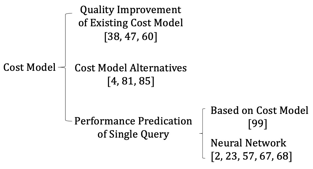
Figure 3. A classification of cost estimation methods

cost estimation methods

In this section, we present the researches proposed to solve the limitations in the cost model. We classify the methods into three groups: (1) improving the capability of the existed cost model, (2) building a new cost model, and (3) predicting the query performance. We include the work on the single query performance prediction. Because the cost used in the optimizer is the metric for performance. These methods are possibly integrated into the cost-based optimizer and replace the cost model to estimation the cost of a (sub)plan, like in (Marcus et al., 2019). However, we do not consider the query performance prediction under concurrent context (e.g.,  (Zhou et al., 2020)). On the one hand, the concurrent queries existing during the optimization may be quite different with queries during the execution process. On the other hand, it also needs to collect more information than the model predicting the performance of a single query. We list the representative work of in the cost model in Figure 3.

4.1. Quality Improvement of Existing Cost Model

Several studies try to estimate the cost of UDF (Boulos and Ono, 1999; He et al., 2004, 2005). Boulos and Ono (1999) execute the UDF several times with different input values, collect the different costs, and then use these costs to build a multi-dimensional histogram. The histogram is stored in a tree structure. When estimating the UDF with specific parameters, traverse the tree top-down to get the estimated cost to locate the leaf with similar parameters with inputs. However, this method needs to know the upper and lower bounds of every parameter and it cannot solve the complex relation between input parameters and the costs. Unlike the static histogram used in (Boulos and Ono, 1999), He et al. (2004) introduce a dynamic quadtree-based approach to store the UDF execution information. When a query is executed, the actual cost of executing the UDF is used to update the cost model. He et al. (2005) introduce a memory-limited K-nearest neighbors (MLKNN) method. They design a data structure, called PData, to store the execution cost and a multidimensional index used for fast retrieval k nearest PData for a given query point (parameter in UDF) and fast insertion of new PData.

Liu and Blanas (2015) introduce a cost model for hash-based join for main-memory database. They model the response time of a query as being proportional to the number of operations weighted by the costs of four basic access patterns. They first adopt the microbenchmarks to get the cost of each access pattern and then model the cost of sequential scan, hash join, hash join with different orders by the basic access patterns.

Most of the previous cost models only consider the execution cost, which may be not reasonable in the cloud environments. The users of the cloud database systems care about the economic cost. Karampaglis et al. (2014) first propose a bi-objective query cost model, which is used to derive running time and monetary cost together in the multi-cloud environment. They model the execution time based on the method in (Wu et al., 2013). For economic cost estimation, they first model the charging policies and estimate the monetary cost by combining the policy and time estimation.

4.2. Cost Model Alternatives

The cost model is a function mapping the (sub)plan with annotated information to a scalar (cost). Because a neural network on data primarily approximates the unknown underlying mapping function from inputs to outputs, most of the methods used to replace the origin cost model are learning-based, especially NN-based.

Boulos et al. (1997) firstly introduce the neural network for cost evaluation. They design two different models: a single large neural network for every query type and a single small neural network for every operator. In the first model, they also train another model to classify a query in a certain type. The output of the first model is the cost of a (sub)plan, while the second model needs to add up the outputs from small models to get the cost.

Sun and Li (2020) adopt a tree-LSTM model to learn the presentation of an operator and add an estimation layer upon the tree-LSTM model to estimate the cost of the query plan.

Due to the difficulty in collecting statistics and the needs of picking the resources in big data systems, particularly in modern cloud data services, Siddiqui et al. (2020) propose a learning-based cost model and integrate it into the optimizer of SCOPE (Chaiken et al., 2008). They build large number of small models to predict the costs of common (sub)queries, which are extracted from the workload history. The features encoded into the models are quite similar with (Wu et al., 2018). Moreover, to support resource-aware query planning, they add number of partitions allocated to the operator into the features. In order to improve the coverage of the models, they introduce operator-input models and operator-subgraphApprox models and employ a meta-ensemble model to combine the models above as the final model.

4.3. Query Performance Prediction

The performance of the one query mainly refers to the latency. Wu et al. (2013) adopt an offline profiling to calibrate the coefficients in the cost model under a specific hardware and software conditions. Then, they adopt the sampling method to obtain the true cardinalities of the physical operators to predict the execution times.

Ganapathi et al. (2009) adopt the Kernel Canonical Correlation Analysis (KCCA) into the resource estimation, e.g. CPU time. They only model the plan level information, e.g. the number of each physical operator type and their cardinality, which is too vulnerable.

To estimate the resources (CPU time and logical I/O times), Li et al. (2012) train a boosted regression tree for every operator in the database and the consumption of the plan is the sum of the operators’. To make the model more robust, they train a separate scaling function for every operator and combine scaling functions with the regression models to handle the cases when the data distribution, size or queries’ parameters are quite different with the training data. Different with (Ganapathi et al., 2009), this is an operator-level model.

Akdere et al. (2012) propose the learning-based models to predict the query performance. They first design a plan-level model if the workload is known in advance and an operator-level model. Considering the plan-level model makes highly accurate prediction and the operator-level generalizes well, for queries with low operator-level prediction accuracy, they train models for specific query subplans using plan-level modeling and compose both types of models to predict the performance of the entire plan. However, the models adopted are linear.

Marcus and Papaemmanouil (2019) introduce a plan-structure neural network to predict the query’s latency. They design a small neural network, called neural unit, for every logic operator and any instance of the same logic operator shares the same network. Then, these neural units are combined into a tree shape according to the plan tree. The output of one neural unit consists of two parts, the latency of current operator and the information sent to its parent node. The latency of the root neural unit of a plan is the plan’s latency.

Neo (Marcus et al., 2019) is a learning-based query optimizer, which introduces a neural network, called value network, to estimate the latency of (sub)plan. The query-level encoding (join graph and columns with predicts) is fed through several full-connected layers and then concatenated with the plan level encoding, which is a tree vector to represent the physical plan. Next, the concatenated vector is fed into a Tree Convolution and another several full-connected layers to predict the latency of the input physical plan.

4.4. Our Insights

4.4.1. Summaries

The methods trying to improve the existing cost model focus on different aspects, e.g., UDFs, hash join in main memory. These studies leave us an important lesson: when introducing a new logical or physical operator, or re-implementing the existing physical operators, we should consider how to add them into the optimization process and design the corresponding cost estimation formulas for them (e.g., (Leeka and Rajan, 2019; Nam et al., 2020)).

Leaning-based methods adopt the model to capture the complex relationship between cost and the factors while the traditional cost model is defined as a certain formula by the database experts. The NN-based methods used to predict the performance, estimate cost, and estimate cardinality in Section 3.3.1 are quite similar in the features and models selection. For example, Sun and Li (2020) use the same model to estimate the cost and cardinality and Neo (Marcus et al., 2019) uses the latency (performance) of (sub)plan as the cost. A model, which is able to capture the data itself, operator level information, and subplan information, can predict the cost accurately. For example, the work (Sun and Li, 2020), one of the state-of-the-art methods, adopts the tree-LSTM model to capture the information mentioned above. However, all of them are supervised methods. If the workload shifts or the data is updated the models need to be retrained from the scratch.

4.4.2. Possible Future Directions

There are two possible directions as follows:

1. Cloud database systems. The users of the cloud database systems need to meet their latency or throughput at the lowest price. Integrating the economic cost of running queries into the cost model is a possible direction. It is interesting to consider these related information into the cost model. For example, Siddiqui et al. (2020) consider the number of container into their cost model.

2. Learning-based methods. Learning-based methods to estimate the cost also suffer from the same problems with methods in cardinality estimation (Section 3.4.2). The model that has been adopted in a real system is a light model (Siddiqui et al., 2020). The trade-off between accuracy and training time is still a problem. The possible solutions adopted in cardinality estimation also can be used in the cost model.

5. Plan Enumeration

In this section, we present the researches published to handle the problems in plan enumeration. We classify the work on plan enumeration into two groups, non-learning methods and learning-based methods.

5.1. Non-learning Methods

In 1997, Steinbrunn et al. (1997) proposed a representative survey for selecting an optimal join orders. Thus, we mainly focus on the researches after 1997.

5.1.1. Dynamic Programming

Selinger et al. (1979) propose a dynamic programming algorithm to select the optimal join order for a given conjunctive query. They generate the plan in the order of increasing size and restrict the search space to left-deep trees, which significantly speeds up the optimization. Vance and Maier (1996) propose a dynamic programming algorithm to find the optimal join order by considering different partial table sets. They use it to generate the optimal bushy tree join trees containing cross products.  (Selinger et al., 1979; Vance and Maier, 1996) are generate-and-test paradigm and most of the operations are used to check whether the subgraphs are connected and two subgraphs are combinative. Thus, none of them meet the lower bound in (Ono and Lohman, 1990). Moerkotte and Neumann (2006) propose a graph-based Dynamic programming algorithm. They first introduce a graph-based method to generate the connected subgraph. Thus, it does not need to check out the connection and combinations and perform more efficiently. Then, they adopt DP over them for the generation of optimal bushy tree without cross products. Moerkotte and Neumann (2008) extend the method in (Moerkotte and Neumann, 2006) to deal with non-inner joins and a more generalized graph, hyper graph, where join predicates can involve more than two relations.

5.1.2. Top-down Strategies

TDMinCutLazy is the first efficient top-down join enumeration algorithm proposed by DeHaan and Tompa (2007). They utilize the idea of minimal cuts to partition a join graph and introduce two different pruning strategies, predicted cost bounding and accumulated cost bounding into top-down partitioning search, which can avoid exhaustive enumeration. Top-down method is almost as efficient as dynamic programming and has other tempting properties, e.g., pruning, interesting order. Fender and Moerkotte (2011) propose an alternative top-down join enumeration strategy (TDMinCutBranch). TDMinCutBranch introduces a graph-based enumeration strategy which only generates the valid join, i.e. cross-product free partitions, unlike TDMinCutLazy which adopts a generate-and-test approach. In the following year, Fender et al. (2012) propose another top-down enumeration strategy TDMinCutConservative which is easier to implement and gives better runtime performance in comparison to TDMinCutBranch. Furthermore, Fender and Moerkotte (2013a, b) present a general framework to handle non-inner joins and a more generalized graph, hyper graph for top-down join enumeration. RS-Graph, a new join transformation rules based on top-down join enumeration, is presented in (Shanbhag and Sudarshan, 2014) to efficiently generate the space of cross-product free join trees.

5.1.3. Large Queries

For large queries, Greedy Operator Ordering (Fegaras, 1998) builds the bushy join trees bottom-up by adding the most profitable (with the smallest intermediate join size) joins first. To support large queries, Kossmann and Stocker (2000) propose two different incremental dynamic programming methods, IDP-1 and IDP-2. With a given size k, IDP-1 runs the algorithm in (Selinger et al., 1979) to construct the cheapest plan with that size and then regards it as a base relation, and repeats the process. With a given size k, in every iteration, IDP-2 first performs a greedy algorithm to construct the join tree with k tables and then runs DP on the generated join tree to produce the optimal plan, regards the plan as a base relation, and then repeats the process. Neumann (2009) proposes a two-stage algorithm: First, it performs the query simplification to restrict the query graph by the greedy heuristic until the graph becomes tractable for DP, and then it runs a DP algorithm to find the optimal join orders for the simplified the join graph. Bruno et al. (2010) introduce enumerate-rank-merge framework which generalizes and extends the previous heuristics (Fegaras, 1998; Swami, 1989). The enumeration step considers the bushy trees. The ranking step is used to evaluate the best join pair each step, which adopts the min-size metric. The merging step constructs the selected join pair. Neumann and Radke (2018) divide the queries into three types: small queries, medium, and large queries according to their query graph type and the number of tables. Then, they adopt DP to solve small queries, restrict the DP by linearizing the search space for medium queries, and use the idea in (Kossmann and Stocker, 2000) for large queries.

5.1.4. Others

Trummer and Koch (2017) transform the join ordering problem into a mixed integer linear program to minimize the cost of the plan and adopt the existing the MILP solvers to obtain a linear join tree (left-deep tree). To satisfy the linear properties in MILP, they approximate the cost of scan and join operations via linear functions.

Most of existed OLAP systems mainly focus on start/snowfake join queries (PK-FK join relation) and generate the left-deep binary join tree. When handling FK-FK join, like in TPC-DS (snowstorm schema), they inccur a large number of intermediate results. Nam et al. (2020) introduce a new n-ary join operator, which extends the plan space. They define the core graph to represent the FK-FK joins in the join graph and adopt the n-ary join operator to process it. They design a new cost model for this operator and integrate it into an existed OLAP systems.

5.2. Learning-based Methods

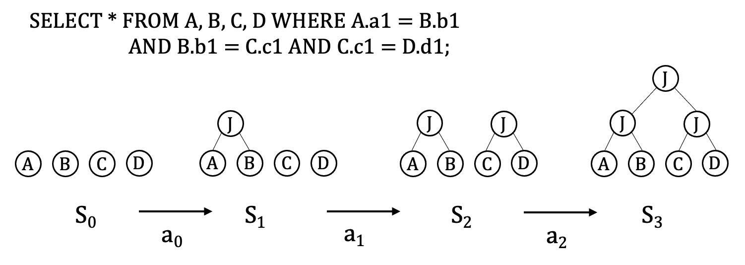
Figure 4. One possible join order episode

RL methods

All learning-based methods adopt the reinforcement learning (DL). In RL, an agent interacts with environment by actions and rewards. At each step $t$, the agent uses a policy $\pi$ to choose an action $a_{t}$ according to the current state $s_{t}$ and transitions to a new state $s_{t+1}$. Then the environment applies the action $a_{t}$ and returns a reward $r_{t}$ to the agent. The goal of RL is to learn a policy $\pi$, a function that automatically takes an action based on the current state, with the maximum long-term reward. In join order selection, state is the current sub-trees, and action is to combine two sub-trees, like in Figure 4. The reward of intermediate action is 0 and the reward of the last action is the cost or latency of the query.

ReJoin (Marcus and Papaemmanouil, 2018) adopts the deep reinforcement learning (DRL), which has widely been adopted in other areas, e.g., influence maximization (Tian et al., 2020), to identify the optimal join orders. State in DRL represent the current subtrees. Each action will combine two subtrees together into a single tree. It uses cost obtained from the cost model in optimizer as the reward. ReJoin encodes the tree structure of (sub)plan, join predicates, and selection predicates in state. Different with (Marcus and Papaemmanouil, 2018), Heitz and Stockinger (2019) create a matrix to represent a table or a subquery in each row and adopt the cost model in (Leis et al., 2015) to quickly obtain the cost of one query. DQ (Krishnan et al., 2018) is also a DRL-based method. It uses one-hot vectors to encode the visible attributes in the (sub)query. DQ also encodes the choice of physical operator by adding another one-hot vector. When training the model, DQ first uses the cost observed from the cost model of the optimizer and then fine-tunes the model with true running time. Yu et al. (2020) adopt DRL and tree-LSTM together for join order selection. Different with the previous methods (Marcus and Papaemmanouil, 2018; Heitz and Stockinger, 2019; Krishnan et al., 2018), tree-LSTM can capture more the structure information of the query tree. Similar with (Krishnan et al., 2018), they also use cost to train the model and then switch to running time as feedback for fine-tuning. Notice, they also discuss how to handle the changes in the database schema, e.g. adding/deleting the tables/columns. SkinnerDB (Trummer et al., 2019) adopts the UCT, a reinforcement learning algorithm, and learns from the current query, while the previous learning-based join order methods are learning from previous queries. It divides the execution of one query into many small slices where different small slices may choose the different join order and learn from the previous execution slices.

5.3. Our Insights

5.3.1. Summaries

The non-learning based studies focus on improving the efficiency and the ability (to handle the more general join cases) of the existing approaches. Compared with dynamic programming approach, the top-down strategy is tempting due to the better extensibility, e.g., adding new transformation rules, branch-and-bound pruning. Both of them have been implemented in many database systems.

Compared with the non-leaning methods, learning-based approaches have a fast planning time. All learning-based methods employ reinforcement learning. The main differences between them are:(1) choosing which information as the state and how to encode them, (2) adopting which models. A more complicated model with more related information can achieve better performance. The state-of-the-art method (Yu et al., 2020) adopts a tree-LSTM model similar with (Sun and Li, 2020) to generate the representation of a subplan. Due to the inaccuracy in the cost model, it can improve the quality of model by using the latency to fine-tune the model. Although current state-of-the-art method (Yu et al., 2020) outperforms the non-learning based methods as shown in their experiments, how to integrate the learning-based method into the real system must be solved.

5.3.2. Possible Future Directions

There are two possible directions as follows:

1. Handle large queries. All methods proposed to handle large queries are DP-based methods in the bottom-up manner. A question is remaining: how to make the top-down search strategy support the large queries. Besides, the state-of-art method for large queries (Neumann and Radke, 2018) cannot support the general join cases.

2. Learning-based methods. Current leaned methods only focus on the PK-FK join and the join type is inner join. How to handle the other join cases is a possible direction. None of the proposed methods have discussed how to integrate them into a real system. In their experiments, they implement the method as a separate component to get the right join order, and then send to the database. The database still need to optimize it to get the final physical plan. If a query has subquery, they may interact multiple times. The reinforcement learning methods are trained in a certain environment, which refers to a certain database in the join order selection problem. How to handle the changes in the table schemas and data is also a possible direction.

6. Conclusion

Cardinality estimation, cost model, and plan enumeration play critical roles to generate an optimal execution plan in a cost-based optimizer. In this paper, we review the work proposed to improve their qualities, including the traditional and learning-based methods. Besides, we provide possible future directions respectively.

We observe that more and more learning-based methods are introduced and outperform traditional methods. However, they suffer from long training and updating time. How to make the models robust to workload shifts and data changes or to update models quickly is still an open question. Traditional methods with theoretical guarantees are widely adopted in real systems. There is a great possibility of improving traditional methods with new algorithms and data structures. Moreover, We believe the ideas behind the traditional methods can be used to enhance the learning-based methods.

- (1)
- Acharya et al. (2015) Jayadev Acharya, Ilias Diakonikolas, Chinmay Hegde, Jerry Zheng Li, and Ludwig Schmidt. 2015. Fast and Near-Optimal Algorithms for Approximating Distributions by Histograms. In PODS. 249–263.
- Akdere et al. (2012) Mert Akdere, Ugur Çetintemel, Matteo Riondato, Eli Upfal, and Stanley B. Zdonik. 2012. Learning-based Query Performance Modeling and Prediction. In ICDE. 390–401.
- Boulos and Ono (1999) Jihad Boulos and Kinji Ono. 1999. Cost Estimation of User-Defined Methods in Object-Relational Database Systems. SIGMOD Rec. 28, 3 (1999), 22–28.
- Boulos et al. (1997) Jihad Boulos, Yann Viemont, and Kinji Ono. 1997. A neural networks approach for query cost evaluation. Transaction of Information Processing Society of Japan 38, 12 (1997), 2566–2575.
- Bruno et al. (2010) Nicolas Bruno, César A. Galindo-Legaria, and Milind Joshi. 2010. Polynomial heuristics for query optimization. In ICDE. 589–600.
- Cai et al. (2019) Walter Cai, Magdalena Balazinska, and Dan Suciu. 2019. Pessimistic Cardinality Estimation: Tighter Upper Bounds for Intermediate Join Cardinalities. In SIGMOD. 18–35.
- Chaiken et al. (2008) Ronnie Chaiken, Bob Jenkins, Per-Åke Larson, Bill Ramsey, Darren Shakib, Simon Weaver, and Jingren Zhou. 2008. SCOPE: easy and efficient parallel processing of massive data sets. VLDB 1, 2 (2008), 1265–1276.
- Chaudhuri (1998) Surajit Chaudhuri. 1998. An Overview of Query Optimization in Relational Systems. In SIGMOD. ACM Press, 34–43.
- Chen and Yi (2017) Yu Chen and Ke Yi. 2017. Two-Level Sampling for Join Size Estimation. In SIGMOD. 759–774.
- Cormode et al. (2012) Graham Cormode, Minos N. Garofalakis, Peter J. Haas, and Chris Jermaine. 2012. Synopses for Massive Data: Samples, Histograms, Wavelets, Sketches. Found. Trends Databases 4, 1-3 (2012), 1–294.
- Cormode and Muthukrishnan (2004) Graham Cormode and S. Muthukrishnan. 2004. An Improved Data Stream Summary: The Count-Min Sketch and Its Applications. In LATIN 2004: Theoretical Informatics, 6th Latin American Symposium, Buenos Aires, Argentina, April 5-8, 2004, Proceedings. 29–38.
- Database (2020) PostgreSQL Database. 2020. http://www.postgresql.org/. Accessed June 10, 2020.
- DeHaan and Tompa (2007) David DeHaan and Frank Wm. Tompa. 2007. Optimal top-down join enumeration. In SIGMOD. 785–796.
- Dutt et al. (2019) Anshuman Dutt, Chi Wang, Azade Nazi, Srikanth Kandula, Vivek R. Narasayya, and Surajit Chaudhuri. 2019. Selectivity Estimation for Range Predicates using Lightweight Models. VLDB 12, 9 (2019), 1044–1057.
- Eavis and Lopez (2007) Todd Eavis and Alex Lopez. 2007. Rk-hist: an r-tree based histogram for multi-dimensional selectivity estimation. In CIKM. 475–484.
- Estan and Naughton (2006) Cristian Estan and Jeffrey F. Naughton. 2006. End-biased Samples for Join Cardinality Estimation. In ICDE. 20.
- Fegaras (1998) Leonidas Fegaras. 1998. A New Heuristic for Optimizing Large Queries. In DEXA. 726–735.
- Fender and Moerkotte (2011) Pit Fender and Guido Moerkotte. 2011. A new, highly efficient, and easy to implement top-down join enumeration algorithm. In ICDE. 864–875.
- Fender and Moerkotte (2013a) Pit Fender and Guido Moerkotte. 2013a. Counter Strike: Generic Top-Down Join Enumeration for Hypergraphs. VLDB 6, 14 (2013), 1822–1833.
- Fender and Moerkotte (2013b) Pit Fender and Guido Moerkotte. 2013b. Top down plan generation: From theory to practice. In ICDE. 1105–1116.
- Fender et al. (2012) Pit Fender, Guido Moerkotte, Thomas Neumann, and Viktor Leis. 2012. Effective and Robust Pruning for Top-Down Join Enumeration Algorithms. In ICDE. 414–425.
- Flajolet et al. (2007) Philippe Flajolet, Eric Fusy, Olivier Gandouet, and Frederic Meunier. 2007. HyperLogLog: the analysis of a near-optimal cardinality estimation algorithm. Discrete Mathematics and Theoretical Computer Science (2007), 137–156.
- Ganapathi et al. (2009) Archana Ganapathi, Harumi A. Kuno, Umeshwar Dayal, Janet L. Wiener, Armando Fox, Michael I. Jordan, and David A. Patterson. 2009. Predicting Multiple Metrics for Queries: Better Decisions Enabled by Machine Learning. In ICDE. 592–603.
- Ganguly et al. (2004) Sumit Ganguly, Minos N. Garofalakis, and Rajeev Rastogi. 2004. Processing Data-Stream Join Aggregates Using Skimmed Sketches. In EDBT. 569–586.
- Ganguly et al. (1996) Sumit Ganguly, Phillip B. Gibbons, Yossi Matias, and Abraham Silberschatz. 1996. Bifocal Sampling for Skew-Resistant Join Size Estimation. In SIGMOD. 271–281.
- Getoor et al. (2001) Lise Getoor, Benjamin Taskar, and Daphne Koller. 2001. Selectivity Estimation using Probabilistic Models. In SIGMOD. 461–472.
- Graefe (1995) Goetz Graefe. 1995. The Cascades Framework for Query Optimization. IEEE Data Eng. Bull. 18, 3 (1995), 19–29.
- Graefe and McKenna (1993) Goetz Graefe and William J. McKenna. 1993. The Volcano Optimizer Generator: Extensibility and Efficient Search. In Proceedings of the Ninth International Conference on Data Engineering, April 19-23, 1993, Vienna, Austria. IEEE Computer Society, 209–218.
- Guha et al. (2006) Sudipto Guha, Nick Koudas, and Kyuseok Shim. 2006. Approximation and streaming algorithms for histogram construction problems. ACM Trans. Database Syst. 31, 1 (2006), 396–438.
- Gunopulos et al. (2005) Dimitrios Gunopulos, George Kollios, Vassilis J. Tsotras, and Carlotta Domeniconi. 2005. Selectivity estimators for multidimensional range queries over real attributes. VLDB J. 14, 2 (2005), 137–154.
- Haas et al. (1993) Peter J. Haas, Jeffrey F. Naughton, S. Seshadri, and Arun N. Swami. 1993. Fixed-Precision Estimation of Join Selectivity. In PODS. 190–201.
- Halford et al. (2019) Max Halford, Philippe Saint-Pierre, and Franck Morvan. 2019. An Approach Based on Bayesian Networks for Query Selectivity Estimation. In DASFAA. 3–19.
- Halim et al. (2009) Felix Halim, Panagiotis Karras, and Roland H. C. Yap. 2009. Fast and effective histogram construction. In CIKM. 1167–1176.
- Halim et al. (2010) Felix Halim, Panagiotis Karras, and Roland H. C. Yap. 2010. Local Search in Histogram Construction. In AAAI.
- Harmouch and Naumann (2017) Hazar Harmouch and Felix Naumann. 2017. Cardinality Estimation: An Experimental Survey. Proc. VLDB Endow. 11, 4 (2017), 499–512.
- Hasan et al. (2020) Shohedul Hasan, Saravanan Thirumuruganathan, Jees Augustine, Nick Koudas, and Gautam Das. 2020. Deep Learning Models for Selectivity Estimation of Multi-Attribute Queries. In SIGMOD. 1035–1050.
- He et al. (2004) Zhen He, Byung Suk Lee, and Robert R. Snapp. 2004. Self-tuning UDF Cost Modeling Using the Memory-Limited Quadtree. In EDBT, Vol. 2992. 513–531.
- He et al. (2005) Zhen He, Byung Suk Lee, and Robert R. Snapp. 2005. Self-tuning cost modeling of user-defined functions in an object-relational DBMS. TODS 30, 3 (2005), 812–853.
- Heimel et al. (2015) Max Heimel, Martin Kiefer, and Volker Markl. 2015. Self-Tuning, GPU-Accelerated Kernel Density Models for Multidimensional Selectivity Estimation. In SIGMOD. 1477–1492.
- Heitz and Stockinger (2019) Jonas Heitz and Kurt Stockinger. 2019. Join Query Optimization with Deep Reinforcement Learning Algorithms. CoRR abs/1911.11689 (2019).
- Hilprecht et al. (2020) Benjamin Hilprecht, Andreas Schmidt, Moritz Kulessa, Alejandro Molina, Kristian Kersting, and Carsten Binnig. 2020. DeepDB: Learn from Data, not from Queries! VLDB 13, 7 (2020), 992–1005.
- Ibaraki and Kameda (1984) Toshihide Ibaraki and Tiko Kameda. 1984. On the Optimal Nesting Order for Computing N-Relational Joins. ACM Trans. Database Syst. 9, 3 (1984), 482–502.
- Indyk et al. (2012) Piotr Indyk, Reut Levi, and Ronitt Rubinfeld. 2012. Approximating and testing k-histogram distributions in sub-linear time. In PODS. 15–22.
- Ioannidis (2003) Yannis E. Ioannidis. 2003. The History of Histograms (abridged). In VLDB. Morgan Kaufmann, 19–30.
- Jagadish et al. (1998) H. V. Jagadish, Nick Koudas, S. Muthukrishnan, Viswanath Poosala, Kenneth C. Sevcik, and Torsten Suel. 1998. Optimal Histograms with Quality Guarantees. In VLDB. 275–286.
- Kaoudi et al. (2020) Zoi Kaoudi, Jorge-Arnulfo Quiané-Ruiz, Bertty Contreras-Rojas, Rodrigo Pardo-Meza, Anis Troudi, and Sanjay Chawla. 2020. ML-based Cross-Platform Query Optimization. In ICDE. 1489–1500.
- Karampaglis et al. (2014) Zisis Karampaglis, Anastasios Gounaris, and Yannis Manolopoulos. 2014. A Bi-objective Cost Model for Database Queries in a Multi-cloud Environment. In MEDES. 109–116.
- Kaushik and Suciu (2009) Raghav Kaushik and Dan Suciu. 2009. Consistent Histograms In The Presence of Distinct Value Counts. VLDB 2, 1 (2009), 850–861.
- Kiefer et al. (2017) Martin Kiefer, Max Heimel, Sebastian Breß, and Volker Markl. 2017. Estimating Join Selectivities using Bandwidth-Optimized Kernel Density Models. VLDB 10, 13 (2017), 2085–2096.
- Kipf et al. (2019a) Andreas Kipf, Thomas Kipf, Bernhard Radke, Viktor Leis, Peter A. Boncz, and Alfons Kemper. 2019a. Learned Cardinalities: Estimating Correlated Joins with Deep Learning. In CIDR.
- Kipf et al. (2019b) Andreas Kipf, Dimitri Vorona, Jonas Müller, Thomas Kipf, Bernhard Radke, Viktor Leis, Peter A. Boncz, Thomas Neumann, and Alfons Kemper. 2019b. Estimating Cardinalities with Deep Sketches. CoRR abs/1904.08223 (2019).
- Kossmann and Stocker (2000) Donald Kossmann and Konrad Stocker. 2000. Iterative dynamic programming: a new class of query optimization algorithms. TODS 25, 1 (2000), 43–82.
- Krishnan et al. (2018) Sanjay Krishnan, Zongheng Yang, Ken Goldberg, Joseph M. Hellerstein, and Ion Stoica. 2018. Learning to Optimize Join Queries With Deep Reinforcement Learning. CoRR abs/1808.03196 (2018).
- Lakshmi and Zhou (1998) M. Seetha Lakshmi and Shaoyu Zhou. 1998. Selectivity Estimation in Extensible Databases - A Neural Network Approach. In VLDB. 623–627.
- Leeka and Rajan (2019) Jyoti Leeka and Kaushik Rajan. 2019. Incorporating Super-Operators in Big-Data Query Optimizers. VLDB 13, 3 (2019), 348–361.
- Leis et al. (2015) Viktor Leis, Andrey Gubichev, Atanas Mirchev, Peter A. Boncz, Alfons Kemper, and Thomas Neumann. 2015. How Good Are Query Optimizers, Really? VLDB 9, 3 (2015), 204–215.
- Li et al. (2012) Jiexing Li, Arnd Christian König, Vivek R. Narasayya, and Surajit Chaudhuri. 2012. Robust Estimation of Resource Consumption for SQL Queries using Statistical Techniques. VLDB 5, 11 (2012), 1555–1566.
- Lim et al. (2003) Lipyeow Lim, Min Wang, and Jeffrey Scott Vitter. 2003. SASH: A Self-Adaptive Histogram Set for Dynamically Changing Workloads. In VLDB. 369–380.
- Lin et al. (2015) Xudong Lin, Xiaoning Zeng, Xiaowei Pu, and Yanyan Sun. 2015. A Cardinality Estimation Approach Based on Two Level Histograms. J. Inf. Sci. Eng. 31, 5 (2015), 1733–1756.
- Liu and Blanas (2015) Feilong Liu and Spyros Blanas. 2015. Forecasting the cost of processing multi-join queries via hashing for main-memory databases. In Socc. 153–166.
- Liu et al. (2015) Henry Liu, Mingbin Xu, Ziting Yu, Vincent Corvinelli, and Calisto Zuzarte. 2015. Cardinality estimation using neural networks. In CASCON. 53–59.
- Lohman (2014) Guy Lohman. 2014. IS QUERY OPTIMIZATION A “SOLVED” PROBLEM? http://wp.sigmod.org/?p=1075. Accessed June 10, 2020.
- Ma et al. (2020) Lin Ma, Bailu Ding, Sudipto Das, and Adith Swaminathan. 2020. Active Learning for ML Enhanced Database Systems. In SIGMOD. 175–191.
- Malik et al. (2007) Tanu Malik, Randal C. Burns, and Nitesh V. Chawla. 2007. A Black-Box Approach to Query Cardinality Estimation. In CIDR. 56–67.
- Manegold et al. (2002) Stefan Manegold, Peter A. Boncz, and Martin L. Kersten. 2002. Generic Database Cost Models for Hierarchical Memory Systems. In VLDB. 191–202.
- Marcus and Papaemmanouil (2018) Ryan Marcus and Olga Papaemmanouil. 2018. Deep Reinforcement Learning for Join Order Enumeration. In aiDM@SIGMOD. 3:1–3:4.
- Marcus et al. (2019) Ryan C. Marcus, Parimarjan Negi, Hongzi Mao, Chi Zhang, Mohammad Alizadeh, Tim Kraska, Olga Papaemmanouil, and Nesime Tatbul. 2019. Neo: A Learned Query Optimizer. VLDB 12, 11 (2019), 1705–1718.
- Marcus and Papaemmanouil (2019) Ryan C. Marcus and Olga Papaemmanouil. 2019. Plan-Structured Deep Neural Network Models for Query Performance Prediction. VLDB 12, 11 (2019), 1733–1746.
- Moerkotte and Neumann (2006) Guido Moerkotte and Thomas Neumann. 2006. Analysis of Two Existing and One New Dynamic Programming Algorithm for the Generation of Optimal Bushy Join Trees without Cross Products. In VLDB. 930–941.
- Moerkotte and Neumann (2008) Guido Moerkotte and Thomas Neumann. 2008. Dynamic programming strikes back. In SIGMOD. 539–552.
- Nam et al. (2020) Yoon-Min Nam, Donghyoung Han, and Min-Soo Kim. 2020. SPRINTER: A Fast n-ary Join Query Processing Method for Complex OLAP Queries. In SIGMOD. 2055–2070.
- Neumann (2009) Thomas Neumann. 2009. Query simplification: graceful degradation for join-order optimization. In SIGMOD. 403–414.
- Neumann and Radke (2018) Thomas Neumann and Bernhard Radke. 2018. Adaptive Optimization of Very Large Join Queries. In SIGMOD. 677–692.
- Ono and Lohman (1990) Kiyoshi Ono and Guy M. Lohman. 1990. Measuring the Complexity of Join Enumeration in Query Optimization. In VLDB. 314–325.
- Ortiz et al. (2019) Jennifer Ortiz, Magdalena Balazinska, Johannes Gehrke, and S. Sathiya Keerthi. 2019. An Empirical Analysis of Deep Learning for Cardinality Estimation. CoRR abs/1905.06425 (2019).
- Park et al. (2020) Yongjoo Park, Shucheng Zhong, and Barzan Mozafari. 2020. QuickSel: Quick Selectivity Learning with Mixture Models. In SIGMOD. 1017–1033.
- Poosala et al. (1996) Viswanath Poosala, Yannis E. Ioannidis, Peter J. Haas, and Eugene J. Shekita. 1996. Improved Histograms for Selectivity Estimation of Range Predicates. In SIGMOD. 294–305.
- Rusu and Dobra (2008) Florin Rusu and Alin Dobra. 2008. Sketches for size of join estimation. ACM Trans. Database Syst. 33, 3 (2008), 15:1–15:46.
- Selinger et al. (1979) Patricia G. Selinger, Morton M. Astrahan, Donald D. Chamberlin, Raymond A. Lorie, and Thomas G. Price. 1979. Access Path Selection in a Relational Database Management System. In SIGMOD. 23–34.
- Shanbhag and Sudarshan (2014) Anil Shanbhag and S. Sudarshan. 2014. Optimizing Join Enumeration in Transformation-based Query Optimizers. VLDB 7, 12 (2014), 1243–1254.
- Siddiqui et al. (2020) Tarique Siddiqui, Alekh Jindal, Shi Qiao, Hiren Patel, and Wangchao Le. 2020. Cost Models for Big Data Query Processing: Learning, Retrofitting, and Our Findings. In SIGMOD. 99–113.
- Spiegel and Polyzotis (2006) Joshua Spiegel and Neoklis Polyzotis. 2006. Graph-based synopses for relational selectivity estimation. In SIGMOD. 205–216.
- Srivastava et al. (2006) Utkarsh Srivastava, Peter J. Haas, Volker Markl, Marcel Kutsch, and Tam Minh Tran. 2006. ISOMER: Consistent Histogram Construction Using Query Feedback. In ICDE. 39.
- Steinbrunn et al. (1997) Michael Steinbrunn, Guido Moerkotte, and Alfons Kemper. 1997. Heuristic and Randomized Optimization for the Join Ordering Problem. VLDB J. 6, 3 (1997), 191–208.
- Sun and Li (2020) Ji Sun and Guoliang Li. 2020. An End-to-End Learning-based Cost Estimator. VLDB 13, 3 (2020), 307–319.
- Swami (1989) Arun N. Swami. 1989. Optimization of Large Join Queries: Combining Heuristic and Combinatorial Techniques. In SIGMOD. 367–376.
- Tian et al. (2020) Shan Tian, Songsong Mo, Liwei Wang, and Zhiyong Peng. 2020. Deep Reinforcement Learning-Based Approach to Tackle Topic-Aware Influence Maximization. Data Sci. Eng. 5, 1 (2020), 1–11.
- To et al. (2013) Hien To, Kuorong Chiang, and Cyrus Shahabi. 2013. Entropy-based histograms for selectivity estimation. In CIKM. 1939–1948.
- Trummer and Koch (2017) Immanuel Trummer and Christoph Koch. 2017. Solving the Join Ordering Problem via Mixed Integer Linear Programming. In SIGMOD. 1025–1040.
- Trummer et al. (2019) Immanuel Trummer, Junxiong Wang, Deepak Maram, Samuel Moseley, Saehan Jo, and Joseph Antonakakis. 2019. SkinnerDB: Regret-Bounded Query Evaluation via Reinforcement Learning. In SIGMOD. 1153–1170.
- Tzoumas et al. (2011) Kostas Tzoumas, Amol Deshpande, and Christian S. Jensen. 2011. Lightweight Graphical Models for Selectivity Estimation Without Independence Assumptions. VLDB 4, 11 (2011), 852–863.
- Tzoumas et al. (2013) Kostas Tzoumas, Amol Deshpande, and Christian S. Jensen. 2013. Efficiently adapting graphical models for selectivity estimation. VLDB J. 22, 1 (2013), 3–27.
- Vance and Maier (1996) Bennet Vance and David Maier. 1996. Rapid Bushy Join-order Optimization with Cartesian Products. In SIGMOD. 35–46.
- Vengerov et al. (2015) David Vengerov, Andre Cavalheiro Menck, Mohamed Zaït, and Sunil Chakkappen. 2015. Join Size Estimation Subject to Filter Conditions. VLDB 8, 12 (2015), 1530–1541.
- Wang and Chan (2020) TaiNing Wang and Chee-Yong Chan. 2020. Improved Correlated Sampling for Join Size Estimation. In ICDE. 325–336.
- Woltmann et al. (2020) Lucas Woltmann, Claudio Hartmann, Dirk Habich, and Wolfgang Lehner. 2020. Machine Learning-based Cardinality Estimation in DBMS on Pre-Aggregated Data. CoRR abs/2005.09367 (2020).
- Woltmann et al. (2019) Lucas Woltmann, Claudio Hartmann, Maik Thiele, Dirk Habich, and Wolfgang Lehner. 2019. Cardinality estimation with local deep learning models. In aiDM@SIGMOD. 5:1–5:8.
- Wu et al. (2018) Chenggang Wu, Alekh Jindal, Saeed Amizadeh, Hiren Patel, Wangchao Le, Shi Qiao, and Sriram Rao. 2018. Towards a Learning Optimizer for Shared Clouds. VLDB 12, 3 (2018), 210–222.
- Wu et al. (2013) Wentao Wu, Yun Chi, Shenghuo Zhu, Jun’ichi Tatemura, Hakan Hacigümüs, and Jeffrey F. Naughton. 2013. Predicting query execution time: Are optimizer cost models really unusable?. In ICDE. 1081–1092.
- Wu et al. (2016) Wentao Wu, Jeffrey F. Naughton, and Harneet Singh. 2016. Sampling-Based Query Re-Optimization. In SGMOD. 1721–1736.
- Yang et al. (2019b) Yang Yang, Wenjie Zhang, Ying Zhang, Xuemin Lin, and Liping Wang. 2019b. Selectivity Estimation on Set Containment Search. Data Sci. Eng. 4, 3 (2019), 254–268.
- Yang et al. (2019c) Yang Yang, Wenjie Zhang, Ying Zhang, Xuemin Lin, and Liping Wang. 2019c. Selectivity Estimation on Set Containment Search. In DASFAA, Part I. 330–349.
- Yang et al. (2020) Zongheng Yang, Amog Kamsetty, Sifei Luan, Eric Liang, Yan Duan, Xi Chen, and Ion Stoica. 2020. NeuroCard: One Cardinality Estimator for All Tables. CoRR abs/2006.08109 (2020). arXiv:2006.08109
- Yang et al. (2019a) Zongheng Yang, Eric Liang, Amog Kamsetty, Chenggang Wu, Yan Duan, Peter Chen, Pieter Abbeel, Joseph M. Hellerstein, Sanjay Krishnan, and Ion Stoica. 2019a. Deep Unsupervised Cardinality Estimation. VLDB 13, 3 (2019), 279–292.
- Yu et al. (2013) Feng Yu, Wen-Chi Hou, Cheng Luo, Dunren Che, and Mengxia Zhu. 2013. CS2: a new database synopsis for query estimation. In SIGMOD. 469–480.
- Yu et al. (2020) Xiang Yu, Guoliang Li, Chengliang Chai, and Nan Tang. 2020. Reinforcement Learning with Tree-LSTM for Join Order Selection. In ICDE. 1297–1308.
- Zhou et al. (2020) X. Zhou, C. Chai, G. Li, and J. SUN. 2020. Database Meets Artificial Intelligence: A Survey. TKDE (2020), 1–1.
- Zhou et al. (2020) Xuanhe Zhou, Ji Sun, Guoliang Li, and Jianhua Feng. 2020. Query Performance Prediction for Concurrent Queries using Graph Embedding. VLDB 13, 9 (2020), 1416–1428.