Dynamic sensitivity of quantum Rabi model with quantum criticality

Abstract

We study the dynamic sensitivity of the quantum Rabi model, which exhibits quantum criticality in the finite-component-system case. This dynamic sensitivity can be detected by introducing an auxiliary two-level atom far-off-resonantly coupled to the cavity field of the quantum Rabi model. We find that when the quantum Rabi model goes through the critical point, the auxiliary atom experiences a sudden decoherence, which can be characterised by a sharp decay of the Loschmidt echo. Our scheme will provide a reliable way to observe quantum phase transition in ultrastrongly coupled quantum systems.

I INTRODUCTION

Quantum phase transition (QPT) [1], as a fundamental phenomenon in quantum physics, is characterized by the sudden change of the ground states of quantum systems, induced by the change of system parameters. In general, a quantum system occurred phase transition needs to reach a thermodynamic limit, i.e., the components of the system should attain infinity [2, 3, 4, 5, 6]. Since the infinite-component systems are composed of numerous degrees of freedom, it will take a long time to prepare the initial state of the systems, and the systems are easily affected by their environments. Consequently, an interesting question is whether quantum phase transition can take place in a finite-component system. It has recently been shown that quantum phase transition can take place in simple systems [7, 8, 9, 10, 11, 12, 13, 6, 14, 15, 16, 17, 18, 19, 20, 21]. An advantage of this kind of systems is that the systems have less degrees of freedom, and hence those previous mentioned difficulties in infinite-component systems can be improved [22].

Quantum Rabi model (QRM), as a typical finite-component quantum system, describes the interaction between a single two-level atom (qubit) and a single bosonic mode. As one of the most fundamental models in quantum optics, the QRM has attracted much attention from the communities of quantum physics, quantum information, and especially ultrastrong couplings [23, 24, 25]. In QRM, it has been shown that the quantum criticality exists in a limit case, in which the ratio $\eta=\omega_{0}/\omega_{c}$ of the qubit frequency $\omega_{0}$ to the bosonic-mode frequency $\omega_{c}$ tends to infinity. It has also been recognized that the quantum critical position of the QRM depends on the frequency of the bosonic mode, and that the coupling strength needs to enter the ultrastrong-coupling regime [23, 24, 25]. Currently, with the improvement of the experimental conditions, the ultrastrong couplings even deep-strong couplings have been realized in various physical systems, such as superconducting quantum circuits [25, 26, 27, 28, 29] and semiconductor quantum wells [30, 31, 32]. In the ultrastrong-coupling regime, the coupling strength is comparable to the frequencies of the bosonic mode and the two-level atom. Furthermore, the quantum criticality in finite-component quantum systems has been expected and experimentally demonstrated in trapped-ion systems [33, 34, 35, 36, 37]. All these advances motivate the experimental studies of quantum criticality in various finite-component quantum systems, and hence how to observe quantum criticality in realistic finite-component quantum systems becomes an interesting task.

In this paper, we propose to show the dynamic sensitivity caused by quantum criticality in the QRM by introducing an auxiliary atom coupled to the cavity field of the QRM. Here, the auxiliary atom plays two important roles in this system. The first role is a trigger, which is used to stir up the quantum criticality in this system. The second role is a sensor to detect the quantum critical behavior in the QRM. Here, the decoherence of the auxiliary atom can reflect the dynamic sensitivity of the QRM, and we use the Loschmidt echo (LE) to measure the decoherence of the auxiliary atom [38, 39]. In the short-time limit, the LE can be simplified to an exponential function of the photon number variance in the ground state of the QRM. As a result, we calculate the ground state of QRM in both the normal and superradiance phases, and compare the analytical ground state in the infinite $\eta$ case with the numerical ground state in the finite $\eta$ case [15]. We also analyze the LE of the auxiliary atom and find a dynamic sensitivity around the critical point of the QRM. This feature provides a signature to characterize the quantum criticality in this system.

The rest of this paper is organized as follows. In Sec. II, we introduce the QRM and construct conditional Rabi interactions by introducing an auxiliary two-level atom far-off-resonantly coupled to the cavity field in the QRM. In Sec. III, we present the analytical result for the LE of the auxiliary atom. We also calculate the ground state of the critical QRM when it works in both the normal and the superradiance phases at both finite and infinite $\eta$. In Sec. IV, we exhibit the dependence of the LE on the system parameters and analyze the dynamic sensitivity of the QRM. Finally, a brief summary of this paper is presented in Sec. V.

II MODEL AND HAMILTONIAN

We consider the quantum Rabi model, which is composed of a single-mode cavity field coupled to a two-level atom. The Hamiltonian of the QRM reads ($\hbar=1$) [23, 24]

$$\hat{H}_{\mathrm{Rabi}}=\omega_{c}\hat{a}^{\dagger}\hat{a}+\dfrac{\omega_{0}}{2}\hat{\sigma}_{z}-g\hat{\sigma}_{x}(\hat{a}+\hat{a}^{\dagger}),$$ (1)

where $\hat{a}\ (\hat{a}^{\dagger})$ is the annihilation (creation) operator of the cavity field with resonance frequency $\omega_{c}$. The two-level atom has the ground state $|g\rangle$ and excited state $|e\rangle$ with transition frequency $\omega_{0}$, and it is described by the Pauli operators $\hat{\sigma}_{x}\equiv|e\rangle\langle g|+|g\rangle\langle e|$, $\hat{\sigma}_{y}\equiv i(|g\rangle\langle e|-|e\rangle\langle g|)$, and $\hat{\sigma}_{z}\equiv|e\rangle\langle e|-|g\rangle\langle g|$. The parameter $g$ denotes the coupling strength between the cavity field and the atom. In QRM, the parity operator $\hat{\Pi}=\exp\{i\pi[\hat{a}^{\dagger}\hat{a}+(1+\hat{\sigma}_{z})/2]\}$ is a conserved quantity based on the commutative relation $[\hat{\Pi},\hat{H}_{\mathrm{Rabi}}]=0$, then the Hilbert space of the QRM can be divided into two subspaces with odd and even parities. It is known that the QRM has a $Z_{2}$ parity symmetry and it is integrable [40, 41, 42]. The analytic eigensystem is determined by a transcendental equation given in Refs. [41, 43, 44, 45]. Due to the lack of closed-form solution, several methods for approximatively solving the QRM have also been proposed [46, 47, 48, 49, 50, 16, 51, 52, 53].

It has been found that a QPT takes place in the QRM at the critical point $g=\sqrt{\omega_{c}\omega_{0}}/2$ [15]. This feature motivates us to detect the dynamic sensitivity of quantum criticality in the QRM by introducing an auxiliary atom $S$ coupled to the cavity field of the QRM. The auxiliary atom and its interaction with the cavity field are described by the Hamiltonian

$$\hat{H}_{I}=\dfrac{\omega_{s}}{2}\hat{\sigma}_{z}^{(s)}-g_{s}(\hat{a}^{\dagger}\hat{\sigma}_{-}^{(s)}+\hat{\sigma}_{+}^{(s)}\hat{a}),$$ (2)

where $\hat{\sigma}_{z}^{(s)}=|e\rangle_{\!s\,s\!}\langle e|-|g\rangle_{\!s\,s\!}\langle g|$ is the $z$-direction Pauli operator, $\hat{\sigma}_{+}^{(s)}=|e\rangle_{\!s\,s\!}\langle g|$ and $\hat{\sigma}_{-}^{(s)}=|g\rangle_{\!s\,s\!}\langle e|$ are the raising and lowing operators of the auxiliary atom, respectively. $\omega_{s}$ is the transition frequency between the ground state $|g\rangle_{\!s}$ and excited states $|e\rangle_{\!s}$ of the auxiliary atom. $g_{s}$ is the coupling strength between the cavity field and the auxiliary atom. Note that here we consider the case where the interaction between the auxiliary atom and the cavity field works in the Jaynes-Cummings (JC) coupling regime [54] and then the rotating-wave approximation has been made in Hamiltonian (2).

We assume that the auxiliary two-level atom $S$ is far-off-resonantly coupled with the single-mode cavity field, namely the detuning $\Delta_{s}\equiv\omega_{s}-\omega_{c}$ is much larger than the coupling strength $g_{s}\sqrt{n}$ with $n$ being the involved photon number. In the large-detuning regime, the interaction between the auxiliary atom $S$ and the cavity field is described by the dispersive JC model [55]. Therefore, the Hamiltonian of the whole system including the QRM and the auxiliary atom reads

$$\hat{H}_{\mathrm{eff}}= \ \omega_{c}\hat{a}^{\dagger}\hat{a}+\frac{\omega_{0}}{2}\hat{\sigma}_{z}-g\hat{\sigma}_{x}(\hat{a}+\hat{a}^{\dagger})$$

$$+\frac{1}{2}\omega_{s}\hat{\sigma}_{z}^{(s)}+\chi\hat{\sigma}_{z}^{(s)}\hat{a}^{\dagger}\hat{a}+\chi\hat{\sigma}_{+}^{(s)}\hat{\sigma}_{-}^{(s)},$$ (3)

where $\chi\equiv g_{s}^{2}/\Delta_{s}$ is the dispersive JC coupling strength between the auxiliary atom and the cavity field. The dispersive JC coupling describes a conditional frequency shift for the cavity field. To clearly see the dynamic sensitivity of the finite-component system response to the auxiliary atom, we rewrite Hamiltonian (3) as the following form

$$\hat{H}_{\mathrm{eff}}=\hat{H}_{e}\otimes|e\rangle_{\!s\,s\!}\langle e|+\hat{H}_{g}\otimes|g\rangle_{\!s\,s\!}\langle g|,$$ (4)

where

$$\hat{H}_{e} =\omega_{e}\hat{a}^{\dagger}\hat{a}+\frac{\omega_{0}}{2}\hat{\sigma}_{z}-g\hat{\sigma}_{x}(\hat{a}+\hat{a}^{\dagger})+\frac{\omega_{s}}{2}+\chi,$$ (5)

$$\hat{H}_{g} =\omega_{g}\hat{a}^{\dagger}\hat{a}+\frac{\omega_{0}}{2}\hat{\sigma}_{z}-g\hat{\sigma}_{x}(\hat{a}+\hat{a}^{\dagger})-\frac{\omega_{s}}{2},$$ (6)

with the state-dependent cavity frequencies $\omega_{e}=\omega_{c}+\chi$ and $\omega_{g}=\omega_{c}-\chi$. Note that up to the constant terms, both the two Hamiltonians in Eqs. (5) and (6) describe the QRM with different cavity-field frequencies.

III QUANTUM CRITICAL EFFECT

In this section, we derive the relation between the LE and the photon number variance of the cavity field. We also calculate the expression of the photon number varianance in the finite and infinite $\eta$ cases when the QRM works in both the normal and superradiance phases.

III.1 Expression of the LE

To study quantum critical effect in this system, we investigate the dynamic evolution of the system, which is governed by Hamiltonian (4). To this end, we assume that the QRM is initially in its ground state $|G\rangle$ and the auxiliary atom is in a superposed state $\alpha|g\rangle_{\!s}+\beta|e\rangle_{\!s}$, where $\alpha$ and $\beta$ are the superposition coefficients, satisfying the normalization condition $|\alpha|^{2}+|\beta|^{2}=1$. Corresponding to the auxiliary atom in states $|g\rangle_{\!s}$ and $|e\rangle_{\!s}$, the evolution of the QRM is governed by the Hamiltonians $\hat{H}_{g}$ and $\hat{H}_{e}$, respectively. Then, the state of the total system at time $t$ becomes

$$\left|\Psi(t)\right\rangle=\alpha|g\rangle_{\!s}\otimes|\Phi_{g}(t)\rangle+\beta|e\rangle_{\!s}\otimes|\Phi_{e}(t)\rangle,$$ (7)

where $|\Phi_{g}(t)\rangle\equiv\mathrm{e}^{-i\hat{H}_{g}t}|G\rangle$ and $|\Phi_{e}(t)\rangle\equiv\mathrm{e}^{-i\hat{H}_{e}t}|G\rangle$. The central task of this paper is to study the dynamic sensitivity of the QRM with respect to the state of the auxiliary atom, which could play the role of a sensor to detect the criticality of QRM. To show this physical mechanism, we trace over the degrees of freedom of the QRM, and obtain the reduced density matrix of the auxiliary atom as

$$\hat{\rho}_{s}(t)=|\alpha|^{2}|g\rangle_{\!s\,s\!}\langle g|+|\beta|^{2}|e\rangle_{\!s\,s\!}\langle e|+[D(t)\alpha^{\ast}\beta|e\rangle_{\!s\,s\!}\langle g|+\mathrm{H.c.}],$$ (8)

where the decoherence factor $D(t)$ is defined by

$$D(t)=\langle\Phi_{g}(t)|\Phi_{e}(t)\rangle=\langle G|\mathrm{e}^{i\hat{H}_{g}t}\mathrm{e}^{-i\hat{H}_{e}t}|G\rangle.$$ (9)

To understand the dynamic sensitivity in this finite-component system, we calculate the LE of the auxiliary atom by

$$L(t)=|D(t)|^{2}=|\langle G|\mathrm{e}^{i\hat{H}_{g}t}\mathrm{e}^{-i\hat{H}_{e}t}|G\rangle|^{2}.$$ (10)

In the short-time limit, the LE can be approximated as

$$L(t)\approx\exp(-4\gamma\chi^{2}t^{2}),$$ (11)

where $\gamma=\langle G|(\hat{a}^{\dagger}\hat{a})^{2}|G\rangle-\langle G|\hat{a}^{\dagger}\hat{a}|G\rangle^{2}$ is the photon number variance. Note that the operator average here is taken over the ground state of the QRM. Equation (11) shows that the decay rate of the LE depends on $t^{2}$ and the photon number variance $\gamma$. To obtain the LE, we need to know the ground states of the QRM working in both the normal and the superradiance phases.

The QRM undergoes a quantum phase transition from the normal phase to the superradiance phase by increasing the coupling strength crossing the critical point $g_{c}=\sqrt{\omega_{c}\omega_{0}}/2$. When the QRM goes through the critical point, the ground state of the QRM experience a huge change. In this paper, we will exhibit some special features around the critical point by calculating the photon number variance $\gamma$ in these two phases. When $L(t)$ approaches zero, the QRM will evolve into two orthogonal states $|\Phi_{g}(t)\rangle$ and $|\Phi_{e}(t)\rangle$. This feature could be used as a measurement tool for detecting the state of the auxiliary atom.

III.2 Photon number variance in the normal phase

In this subsection, we calculate the photon number variance $\gamma$ in the ground state of the QRM working in the normal phase. Note that the ground state of the QRM in the infinite and finite $\eta$ cases have been calculated in Ref. [15]. Here, we present the calculation of the ground state for keeping the completeness of this paper.

III.2.1 The infinite $\eta$ case

We first consider the infinite-frequency limit, i.e., the ratio $\eta=\omega_{0}/\omega_{c}$ of the atomic transition frequency $\omega_{0}$ over the cavity-field frequency $\omega_{c}$ approaches infinity. In this case, the quantum criticality has been analytically found in QRM [15]. By introducing the unitary transformation operator $\hat{U}_{\mathrm{np}}=\exp[i(g/\omega_{0})(\hat{a}+\hat{a}^{\dagger})\hat{\sigma}_{y}]$, the Hamiltonian (1) can be transformed to a decoupling form corresponding to the spin subspaces $\mathcal{H}_{e}$ and $\mathcal{H}_{g}$. Keeping the terms up to the second order of $g/\omega_{0}$, the transformed Hamiltonian becomes [15]

$$\hat{H}_{\mathrm{np}} =\hat{U}_{\mathrm{np}}^{\dagger}\hat{H}_{\mathrm{Rabi}}\hat{U}_{\mathrm{np}}$$

$$\approx\omega_{c}\hat{a}^{\dagger}\hat{a}+\frac{\omega_{c}\lambda^{2}}{4}(\hat{a}+\hat{a}^{\dagger})^{2}\hat{\sigma}_{z}+\frac{\omega_{0}}{2}\hat{\sigma}_{z}+\hat{\mathcal{O}}[(g/\omega_{0})^{2}],$$ (12)

where we introduce the dimensionless coupling strength $\lambda=2g/\sqrt{\omega_{0}\omega_{c}}$. Hamiltonian (12) can be diagonalized in terms of the squeezing operator $\hat{S}(r_{\mathrm{np}})=\exp[r_{\mathrm{np}}(\hat{a}^{\dagger 2}-\hat{a}^{2})/2]$ with $r_{\mathrm{np}}(\lambda)=-\frac{1}{4}\ln(1+\lambda^{2}\hat{\sigma}_{z})$. The diagonalized Hamiltonian reads [15]

$$\hat{H}_{\mathrm{np}}^{\mathrm{d}}=\hat{S}^{\dagger}(r_{\mathrm{np}})\hat{H}_{\mathrm{np}}\hat{S}(r_{\mathrm{np}})=\hat{\epsilon}_{\mathrm{np}}\hat{a}^{\dagger}\hat{a}+\hat{E}_{\mathrm{np}},$$ (13)

where we introduce the conditional frequency $\hat{\epsilon}_{\mathrm{np}}=\omega_{c}\sqrt{1+\lambda^{2}\hat{\sigma}_{z}}$ and the spin-state dependent energy $\hat{E}_{\mathrm{np}}=(\hat{\epsilon}_{\mathrm{np}}-\omega_{c}+\omega_{0}\hat{\sigma}_{z})/2$. By finding the minimum energy, the ground state of the diagonalized Hamiltonian (13) in the normal phase is $\text{$|$}0\rangle|g\rangle$. To keep the Hamiltonian $\hat{H}_{\mathrm{np}}^{\mathrm{d}}$ in the low spin subspace to be Hermitian, the coupling strength $g$ should be smaller than $\sqrt{\omega_{0}\omega_{c}}/2$ such that $\lambda<\lambda_{c}=1$, which defines the parameter space of the normal phase. In our model, the cavity frequency $\omega_{c}$ conditionally depends on the states of the auxiliary atom, and hence the atom $S$ can be used as a trigger to induce the criticality in the QRM.

Based on the above analyses, we know that the ground state of the QRM is approximately expressed as [15]

$$|\psi_{\mathrm{np}}^{G}(r_{\mathrm{np}})\rangle=\hat{U}_{\mathrm{np}}\hat{S}(r_{\mathrm{np}})|0\rangle|g\rangle,$$ (14)

where the operators $\hat{U}_{\mathrm{np}}$ and $\hat{S}(r_{\mathrm{np}})$ have been defined before. In the ground state $|\psi_{\mathrm{np}}^{G}\rangle$, the photon number variance in normal phase can be obtained as

$$\gamma_{\mathrm{np}}=\frac{1}{2}\sinh^{2}(2r_{\mathrm{np}})+\frac{g^{2}}{\omega_{0}^{2}}\mathrm{e}^{-2r_{\mathrm{np}}}.$$ (15)

In terms of Eqs. (11) and (15), the analytical result of the LE in the normal phase can be obtained.

III.2.2 The finite $\eta$ case

The above discussions are valid in the infinite $\eta$ case. To beyond this limit case, below we calculate the ground state of the QRM in a large finite $\eta$ case. To this end, we perform a unitary transfomation with the transformation operator

$$\hat{U}_{\mathrm{np}}^{\sigma}=\exp\left\{i\left[\frac{g}{\omega_{0}}(\hat{a}+\hat{a}^{\dagger})-\frac{4g^{3}}{3\omega_{0}^{3}}(\hat{a}+\hat{a}^{\dagger})^{3}\right]\hat{\sigma}_{y}\right\}$$ (16)

to the Hamiltonian $\hat{H}_{\mathrm{Rabi}}$ [15]. Up to the fourth order of $g/\omega_{0}$, the transformed Hamiltonian becomes [15]

$$\hat{\tilde{H}}_{\mathrm{np}}^{\sigma}= \ (\hat{U}_{\mathrm{np}}^{\sigma})^{\dagger}\hat{H}_{\mathrm{Rabi}}\hat{U}_{\mathrm{np}}^{\sigma}$$

$$= \ \omega_{c}\hat{a}^{\dagger}\hat{a}+\frac{g^{2}}{\omega_{0}}(\hat{a}+\hat{a}^{\dagger})^{2}\hat{\sigma}_{z}-\frac{g^{4}}{\omega_{0}^{3}}(\hat{a}+\hat{a}^{\dagger})^{4}\hat{\sigma}_{z}$$

$$+\frac{\omega_{0}}{2}\hat{\sigma}_{z}+\frac{g^{2}\omega_{c}}{\omega_{0}^{3}}+\hat{\mathcal{O}}[(g/\omega_{0})^{4}].$$ (17)

By projecting the effective Hamiltonian (17) into the low spin subspace $\mathcal{H}_{g}$, we obtain

$$\hat{H}_{\mathrm{np}}^{\sigma}= \ \langle g|\hat{\tilde{H}}_{\mathrm{np}}^{\sigma}|g\rangle$$

$$= \ \omega_{c}\hat{a}^{\dagger}\hat{a}-\frac{\omega_{c}\lambda^{2}}{4}(\hat{a}+\hat{a}^{\dagger})^{2}+\frac{\lambda^{4}\omega_{c}^{2}}{16\omega_{0}}(\hat{a}+\hat{a}^{\dagger})^{4}$$

$$-\frac{\omega_{0}}{2}+\frac{\lambda^{2}\omega_{c}^{2}}{4\omega_{0}}.$$ (18)

To know the ground state of the Hamiltonian $\hat{H}_{\mathrm{np}}^{\sigma}$, we adopt the variational method and assume a trial wave function $|\Psi_{\mathrm{np}}^{G}(s_{\mathrm{np}})\rangle=\hat{S}(s_{\mathrm{np}})|0\rangle|g\rangle$, where $\hat{S}$ is a squeezing operator, and $s_{\mathrm{np}}$ is the undetermined variational squeezing parameter [15, 53]. The ground-state energy can be calculated as

$$E_{\mathrm{np}}^{G}(s_{\mathrm{np}})= \ \omega_{c}\sinh^{2}s_{\mathrm{np}}-\frac{\omega_{c}\lambda^{2}}{4}\mathrm{e}^{2s_{\mathrm{np}}}+\frac{3\lambda^{4}\omega_{c}^{2}}{16\omega_{0}}\mathrm{e}^{4s_{\mathrm{np}}}$$

$$-\frac{\omega_{0}}{2}+\frac{\lambda^{2}\omega_{c}^{2}}{4\omega_{0}}.$$ (19)

Here, the second-order derivative of $E_{\mathrm{np}}^{G}(s_{\mathrm{np}})$ with respect to $s_{\mathrm{np}}$ is positive, and then the minimum energy can be obtained by the zero point of the first-order derivative [15], namely

$$\frac{\mathrm{d}E_{\mathrm{np}}^{G}(s_{\mathrm{np}})}{\mathrm{d}s_{\mathrm{np}}}=\ \frac{\omega_{c}}{2\mathrm{e}^{2s_{\mathrm{np}}}}\left[\frac{3\lambda^{4}\mathrm{e}^{6s_{\mathrm{np}}}}{2\eta}+(1-\lambda^{2})\mathrm{e}^{4s_{\mathrm{np}}}-1\right]=0.$$ (20)

By solving Eq. (20), we obtain the only physical solution as

$$s_{\mathrm{np}}=\frac{1}{2}\ln\left\{\mathrm{Re}\left[\frac{\sqrt[3]{A}}{9\lambda^{4}}+\frac{2(\lambda^{2}-1)\eta}{9\lambda^{4}}+\frac{4(\lambda^{2}-1)^{2}\eta^{2}}{9\lambda^{4}\sqrt[3]{A}}\right]\right\},$$ (21)

where we introduce

$$A= \ 9\sqrt{3}\sqrt{243\lambda^{16}\eta^{2}+(\lambda^{6}-3\lambda^{4}+3\lambda^{2}-1)16\lambda^{8}\eta^{4}}$$

$$+243\lambda^{8}\eta+(\lambda^{6}-3\lambda^{4}+3\lambda^{2}-1)8\eta^{3}.$$ (22)

The ground state of QRM in the finite $\eta$ case can be expressed as

$$|\varphi_{\mathrm{np}}^{G}\rangle=\hat{U}_{\mathrm{np}}^{\sigma}\hat{S}(s_{\mathrm{np}})|0\rangle|g\rangle.$$ (23)

Further, the average photon number in the ground state $|\varphi_{\mathrm{np}}^{G}\rangle$ can be calculated as

$$\langle\hat{a}^{\dagger}\hat{a}\rangle_{\mathrm{np}}=\sinh^{2}s_{\mathrm{np}}+\frac{g^{2}}{\omega_{0}^{2}}-\frac{8g^{4}}{\omega_{0}^{4}}\mathrm{e}^{2s_{\mathrm{np}}},$$ (24)

and the photon number variance can be obtained as

$$\gamma^{\prime}_{\mathrm{np}}\approx\frac{1}{2}\sinh^{2}(2s_{\mathrm{np}})+\frac{g^{2}}{\omega_{0}^{2}}\mathrm{e}^{-2s_{\mathrm{np}}}-\frac{8g^{4}\mathrm{e}^{4s_{\mathrm{np}}}}{\omega_{0}^{4}}.$$ (25)

Then the LE can be calculated based on Eqs. (11) and (25).

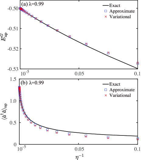
Figure 1: (Color online) (a) and (b) The ground-state energy and the average photon number as functions of the frequency ratio $\eta$ in the normal phase $(\lambda=0.99)$. Here, the exact and approximate results are obtained based on the origin Hamiltonian (1) (black solid line) and the approximate Hamiltonian (18) (squares). The variational results are obtained based on Eqs. (19), (21), and (24) (crosses).

We have used the variational method to solve the effective Hamiltonian and obtained the photon number variance of the ground state in the normal phase at a finite $\eta$. To check the validity of the effective Hamiltonian and the approximate method, in Figs. 1(a) and 1(b) we plot the ground-state energy and the average photon number obtained by the variational and numerical methods, when the QRM works in the normal phase $(\lambda=0.99)$. Meanwhile, we present the exact result based on the origin Hamiltonian (1) for reference. In Fig. 1(a), the ground-state energy obtained by these three methods in the normal phase are consistent with each other in the large $\eta$ case. As the ratio $\eta$ decreases, the deviation between the approximate result and the exact result in the finite $\eta$ case becomes large. However, the variational result agrees well with the numerical result of the effective Hamiltonian. The average photon numbers obtained with these three methods match well in the large $\eta$ case as shown in Fig. 1(b). In contrast, the difference between the variational result and the numerical results increases with the decrease of $\eta$. The reason for this difference is that the trial wave function only preserves the low spin state, and the excite spin state is also important in the finite $\eta$ case. Nevertheless, the variational method can still catch the main physics.

III.3 Photon number variance in the superradiance phase

In this subsection, we calculate the photon number variance $\gamma$ in the ground state of the QRM working in the superradiance phase. Here, we follow some derivations of the ground state of the QRM in the superradiance phase given in Ref. [15] for keeping the completeness of this paper.

III.3.1 The infinite $\eta$ case

Physically, when the light-matter coupling strength increases to be larger than the critical coupling strength, the coupled system will acquire macroscopic excitations. Then the high-order terms which contain the average photon number cannot be ignored. In this case, the approximate Hamiltonian (13) will not be valid as $\lambda>\lambda_{c}$. To achieve the effective Hamiltonian in this case, we introduce a displacement operator $\hat{D}(\alpha)=\exp[\alpha(a^{\dagger}-a)]$ to make a transformation upon Hamiltonian (1) [15]

$$\hat{\tilde{H}}_{\mathrm{Rabi}}(\alpha)= \ \hat{D}^{\dagger}(\alpha)\hat{H}_{\mathrm{Rabi}}\hat{D}(\alpha)$$

$$= \ \omega_{c}(\hat{a}^{\dagger}+\alpha)(\hat{a}+\alpha)-g(\hat{a}+\hat{a}^{\dagger})\hat{\sigma}_{x}$$

$$+\dfrac{\omega_{c}}{2}\hat{\sigma}_{z}-2g\alpha\hat{\sigma}_{x}.$$ (26)

Further, we introduce new spin eigenstates $|\tilde{e}\rangle$ and $|\tilde{g}\rangle$ of the atomic Hamiltonian $\omega_{c}\hat{\sigma}_{z}/2-2g\alpha\hat{\sigma}_{x}$. In terms of the new spin states $|\tilde{e}\rangle=\cos\theta|e\rangle+\sin\theta|g\rangle$ and $|\tilde{g}\rangle=-\sin\theta|e\rangle+\cos\theta|g\rangle$ with $\tan(2\theta)=-4g\alpha/\omega_{0}$, the Pauli operators in the new spin space can be defined by $\hat{\tau}_{0}=|\tilde{e}\rangle\langle\tilde{e}|+|\tilde{g}\rangle\langle\tilde{g}|$, $\hat{\tau}_{x}=|\tilde{e}\rangle\langle\tilde{g}|+|\tilde{g}\rangle\langle\tilde{e}|$, and $\hat{\tau}_{z}=|\tilde{e}\rangle\langle\tilde{e}|-|\tilde{g}\rangle\langle\tilde{g}|$. Then Hamiltonian (26) can be expressed as [15]

$$\hat{\tilde{H}}_{\mathrm{Rabi}}(\alpha)= \ \omega_{c}\hat{a}^{\dagger}\hat{a}-g(\hat{a}+\hat{a}^{\dagger})\cos(2\theta)\hat{\tau}_{x}+\frac{\tilde{\omega}_{0}}{2}\hat{\tau}_{z}+\omega_{c}\alpha^{2}$$

$$+[\omega_{c}\alpha\hat{\tau}_{0}-g\sin(2\theta)\hat{\tau}_{z}](\hat{a}+\hat{a}^{\dagger}).$$ (27)

To eliminate the block-diagonal perturbation term in the subspace $\mathcal{H}_{\tilde{g}}$, we obtain, $\omega_{0}\alpha+g\sin(2\theta)=0$, which leads to the displacement parameters [15]

$$\alpha=\pm\alpha_{\lambda}=\pm\sqrt{\omega_{0}(\lambda^{4}-1)/(4\lambda^{2}\omega_{c})}.$$ (28)

In the infinite-frequency limit, the term $2\omega_{c}\alpha(\hat{a}+\hat{a}^{\dagger})|\tilde{e}\rangle\langle\tilde{e}|$ can be ignored in the new low spin subspace, then the reformulated Hamiltonian becomes [15]

$$\hat{\tilde{H}}_{\mathrm{Rabi}}(\pm\alpha_{\lambda})\approx\omega_{c}\hat{a}^{\dagger}\hat{a}+\frac{\tilde{\omega}_{0}}{2}\hat{\tau}_{z}^{\pm}-\tilde{g}(\hat{a}+\hat{a}^{\dagger})\hat{\tau}_{x}^{\pm}+\omega_{c}\alpha_{\lambda}^{2},$$ (29)

where we introduce the parameters $\tilde{\omega}_{0}=\lambda^{2}\omega_{0}$ and $\tilde{g}=\sqrt{\omega_{c}\omega_{0}}/2\lambda$. The signs “$\pm$” in $\hat{\tau}_{x,z}^{\pm}$ denote the direction of the displacement. Note that the two different signs of the displacement parameter $\alpha$ indicate that the ground state exists twofold degeneracy in QRM [56]. Hamiltonian (29) has a similar structure as that of the QRM, we could use a similar method to obtain the diagonalized Hamiltonian by two unitary transformations as [15]

$$\hat{H}_{\mathrm{sp}}^{\mathrm{d}} =\hat{S}^{\dagger}(r_{\mathrm{sp}})\hat{U}_{\mathrm{sp}}^{\dagger}\hat{\tilde{H}}_{\mathrm{Rabi}}\hat{U}_{\mathrm{sp}}\hat{S}(r_{\mathrm{sp}})$$

$$=\hat{\epsilon}_{\mathrm{sp}}\hat{a}^{\dagger}\hat{a}+\hat{E}_{\mathrm{sp}}$$ (30)

where we introduce the conditional frequency $\hat{\epsilon}_{\mathrm{sp}}=\omega_{c}\sqrt{1+\lambda^{-4}\hat{\tau}_{z}^{\pm}}$ and the new spin-state dependent energy $\hat{E}_{\mathrm{sp}}=(\hat{\epsilon}_{\mathrm{sp}}-\omega_{c}+\omega_{0}\hat{\tau}_{z}^{\pm})/2+\omega_{c}\alpha_{\lambda}^{2}$. The unitary transformation is defined as $\hat{U}_{\mathrm{sp}}=\exp[i(\tilde{g}/\tilde{\omega}_{0})(\hat{a}+\hat{a}^{\dagger})\hat{\tau}_{y}^{\pm}]$, and the squeezing parameter here is $r_{\mathrm{sp}}=-\frac{1}{4}\ln(1+\lambda^{-4}\hat{\tau}_{z}^{\pm})$. The ground state of the diagonalized Hamiltonian (30) in the superradiance phase is $\left|0\right\rangle\left|\tilde{g}^{\pm}\right\rangle$. Similarly, to keep the Hamiltonian $\hat{H}_{\mathrm{sp}}^{\mathrm{d}}$ in the low spin subspace to be Hermitian, the coupling strength $g$ should be larger than $\sqrt{\omega_{0}\omega_{c}}/2$ such that $\lambda>\lambda_{c}=1$, which defines the parameter space of the superradiance phase. The ground state of the QRM in the superradiance phase can be expressed as [15]

$$|\psi_{\mathrm{sp}}^{G}(r_{\mathrm{sp}})\rangle_{\pm}=\hat{D}(\pm\alpha_{\lambda})\hat{U}_{\mathrm{sp}}\hat{S}(r_{\mathrm{sp}})|0\rangle|\tilde{g}^{\pm}\rangle,$$ (31)

where the transformation operators have defined before. In the ground state $|\psi_{\mathrm{sp}}^{G}\rangle_{\pm}$, the photon number variance in the superradiance phase can be obtained as

$$\gamma_{\mathrm{sp}}=\frac{1}{2}\sinh^{2}(2r_{\mathrm{sp}})+\alpha_{\lambda}^{2}\mathrm{e}^{2r_{\mathrm{sp}}}+\frac{\tilde{g}^{2}}{\tilde{\omega}_{0}^{2}}\mathrm{e}^{-2r_{\mathrm{sp}}}.$$ (32)

In terms of Eqs. (11) and (32), the analytical result of the LE in the superradiance phase can be obtained.

III.3.2 The finite $\eta$ case

To beyond the infinite-frequency case, below we calculate the photon number $\gamma_{\mathrm{sp}}^{\prime}$ by the variational method. To this end, we perform a unitary transfomation with the transformation operator

$$\hat{U}_{\mathrm{sp}}^{\sigma}=\exp\left\{i\left[\frac{\tilde{g}}{\tilde{\omega}_{0}}(\hat{a}+\hat{a}^{\dagger})-\frac{4\tilde{g}^{3}}{3\tilde{\omega}_{0}^{3}}(\hat{a}+\hat{a}^{\dagger})^{3}\right]\hat{\tau}_{y}^{\pm}\right\}$$ (33)

to Hamiltonian (29) and projecting the transformed Hamiltonian into the low spin subspace, then the effective Hamiltonian becomes [15]

$$\hat{H}_{\mathrm{sp}}^{\sigma}=\omega_{c}\hat{a}^{\dagger}\hat{a}-\frac{\tilde{g}^{2}}{\tilde{\omega}_{0}}(\hat{a}+\hat{a}^{\dagger})^{2}+\frac{\tilde{g}^{4}}{\tilde{\omega}_{0}^{3}}(\hat{a}+\hat{a}^{\dagger})^{4}-\frac{\tilde{\omega}_{0}}{2}+\frac{\tilde{g}^{2}\omega_{c}}{\tilde{\omega}_{0}^{3}}+\omega_{c}\alpha_{\lambda}^{2}.$$ (34)

Similar to the treatment in the normal-phase case, the trial wave function in the superradiance phase is assumed as $|\Psi_{\mathrm{sp}}^{G}(s_{\mathrm{sp}})\rangle=\hat{S}(s_{\mathrm{sp}})|0\rangle|\tilde{g}^{\pm}\rangle$. The corresponding ground state energy can be obtained as

$$E_{\mathrm{sp}}^{G}(s_{\mathrm{sp}})= \ \omega_{c}\sinh^{2}s_{\mathrm{sp}}-\frac{\omega_{c}}{4\lambda^{4}}\mathrm{e}^{2s_{\mathrm{sp}}}+\frac{3\omega_{c}^{2}}{16\tilde{\omega}_{0}\lambda^{8}}\mathrm{e}^{4s_{\mathrm{sp}}}$$

$$-\frac{\tilde{\omega}_{0}}{2}+\frac{\omega_{c}^{2}}{4\tilde{\omega}_{0}\lambda^{4}}+\omega_{c}\alpha_{g}^{2},$$ (35)

where the parameter $s_{\mathrm{sp}}$ is determined by the zero point of the first-order derivative,

$$\frac{\mathrm{d}E_{\mathrm{sp}}^{G}(s_{\mathrm{sp}})}{\mathrm{d}s_{\mathrm{sp}}}=\ \frac{\omega_{c}}{2\mathrm{e}^{2s_{\mathrm{np}}}}\left[\frac{3\mathrm{e}^{6s_{\mathrm{sp}}}}{2\eta\lambda^{10}}+(1-\lambda^{-4})\mathrm{e}^{4s_{\mathrm{sp}}}-1\right]=0.$$ (36)

The only physical solution of Eq. (36) is given by

$$s_{\mathrm{sp}}=\frac{1}{2}\ln\left\{\mathrm{Re}\left[\frac{\sqrt[3]{B}}{9}-\frac{2(\lambda^{4}-1)}{9\lambda^{-6}\eta^{-1}}+\frac{4(\lambda^{4}-1)^{2}}{9\sqrt[3]{B}\lambda^{-12}\eta^{-2}}\right]\right\},$$ (37)

where we introduce

$$B= \ 9\sqrt{3}\sqrt{243\lambda^{20}\eta^{2}+(1-\lambda^{12}+3\lambda^{8}-3\lambda^{4})16\lambda^{28}\eta^{4}}$$

$$+243\lambda^{10}\eta+(-\lambda^{12}+3\lambda^{8}-3\lambda^{4}+1)8\lambda^{18}\eta^{3}.$$ (38)

The ground state of QRM in this case can be expressed as

$$|\varphi_{\mathrm{sp}}^{G}(s_{\mathrm{sp}})\rangle=\hat{D}(\pm\alpha_{\lambda})\hat{U}_{\mathrm{sp}}^{\sigma}\hat{S}(s_{\mathrm{sp}})|0\rangle|\tilde{g}^{\pm}\rangle.$$ (39)

Based on the ground state (39), the average photon number in the superradiance phase can be calculated as

$$\langle\hat{a}^{\dagger}\hat{a}\rangle_{\mathrm{sp}}=\sinh^{2}s_{\mathrm{sp}}+\frac{\tilde{g}^{2}}{\tilde{\omega}_{0}^{2}}-\frac{8\tilde{g}^{4}}{3\tilde{\omega}_{0}^{4}}\mathrm{e}^{2s_{\mathrm{sp}}}+\alpha_{g}^{2},$$ (40)

and the photon number variance can be obtained

$$\gamma^{\prime}_{\mathrm{sp}}\approx\frac{1}{2}\sinh^{2}(2s_{\mathrm{sp}})+\frac{\tilde{g}^{2}}{\tilde{\omega}_{0}^{2}}\mathrm{e}^{-2s_{\mathrm{sp}}}+\left(\alpha_{g}^{2}-\frac{8\tilde{g}^{4}\mathrm{e}^{2s_{\mathrm{sp}}}}{3\tilde{\omega}_{0}^{4}}\right)\mathrm{e}^{2s_{\mathrm{sp}}}.$$ (41)

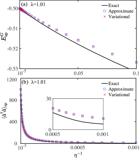
Figure 2: (Color online) (a) and (b) The ground-state energy and the average photon number as functions of the frequency ratio $\eta$ in the superradiance phase $(\lambda=1.01)$. Here, the exact and approximate results are obtained based on the displaced Hamiltonian (26) (black solid line) and the approximate Hamiltonian (34) (squares), respectively. The variational results are obtained based on Eqs. (35), (37), and (40) (crosses).

In order to examine the validity of the effective Hamiltonian (34) and the variational method in the superradiance phase, in Figs. 2(a) and 2(b) we compare the variational result with the numerical result through solving the effective Hamiltonian (34) and the displaced Hamiltonian (26), respectively. In Fig. 2(a), we plot the ground-state energy of the QRM solved based on the exact displaced Hamiltonian, the approximate Hamiltonian, and the variational method. Here, we find that the results based on these three methods match better as the frequency ratio $\eta$ increases. For the average photon number as plotted in Fig. 2(b), we observe that its average value is very large, which corresponds to the characteristics of the system in the superradiance phase. We also see that the variational results match the numerical results well in the superradiance phase (inset), which indicates the validity of the variational method.

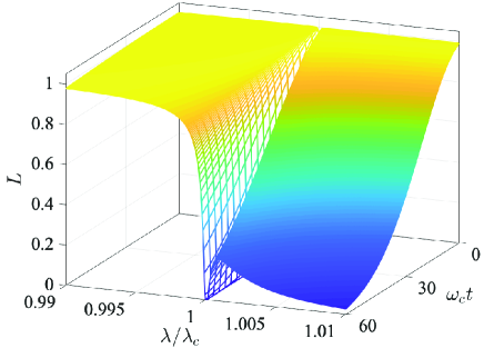
Figure 3: (Color online) The LE of the auxiliary atom as a function of the scaled coupling strength $\lambda/\lambda_{c}$ and the scaled evolution time $\omega_{c}t$ in both the normal phase ($\lambda<\lambda_{c}$) and the superradiance phase ($\lambda>\lambda_{c}$). Here, we take $\eta=5000$ and $\chi=g_{s}^{2}/\Delta_{s}=0.001\omega_{c}$.

By far, we have already calculated the photon number variance of the QRM in both the normal phase and the superradiance phase. In the next section, we will study the LE of the auxiliary atom corresponding to the QRM in the normal and superradiance phases.

IV The LOSCHMIDT ECHO

In this section, we study how to exhibit the critical dynamics of the QRM by checking the LE of the auxiliary atom when the system goes across the critical point from the normal phase to the superradiance phase. In the short-time limit, the LE has been simplified to Eq. (11). Here, the LE can reflect the main character of the QPT by the quantum decoherence of the auxiliary atom. To show the dependence of the LE on the criticality, in Fig. 3 we plot the LE versus the dimensionless coupling strength $\lambda$ and the evolution time $t$ based on Eqs. (11), (15), and (32) in the normal and superradiance phases. Figure 3 shows that, in the vicinity of the critical point, the LE experiences a sharp change within a small range of $\lambda/\lambda_{c}$. In the normal phase, the LE decays sharply to zero as the dimensionless coupling strength $\lambda$ approaches the critical point $\lambda_{c}$. In the superradiance phase, the LE decays faster as the parameter $\lambda$ increases far away from the critical point $\lambda_{c}$, and reaches the minimal value at a large coupling strength. The rapid change indicates that the coherence of the auxiliary atom is supersensitive to a perturbation inflicted on the QRM near the critical point. We can measure the QPT of QRM based on the supersensitive coherence of the auxiliary atom in QRM. In addition, the coherence of the auxiliary atom near the critical point decreases to zero sharply with time at the critical point $\lambda_{c}$. During this process, the detected atom evolves from a pure state to a mixed one.

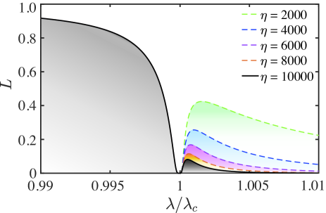
Figure 4: (Color online) The LE of the auxiliary atom versus the scaled coupling strength $\lambda/\lambda_{c}$ at $\omega_{c}t=60$ when $\eta$ takes different values: $\eta=2000$ (green dashed line), $\eta=4000$ (blue dashed line), $\eta=6000$ (purple dashed line), $\eta=8000$ (orange dashed line), and $\eta=10000$ (black solid line). Other parameters used are the same as those given in Fig. 3.

In our previous discussions, we have discussed the ground states of the QRM in both infinite and finite $\eta$ cases. To know the influence of the ratio $\eta$ on the LE, below we study the dependence of the LE on the parameter $\lambda$ at different values of $\eta$. In Fig. 4, the LE is plotted as a function of $\lambda$ at a fixed time when the ratio $\eta$ takes different values: $\eta=2000,4000,6000,8000,$ and $10000$. Here, we can see that, in the normal phase, the LE decays from a finite value to zero when the scaled coupling strength $\lambda/\lambda_{c}$ increases approach to one. In particular, the LE is independent of the ratio $\eta$ in the normal phase. In the superradiance phase, with the increase of the ratio $\lambda/\lambda_{c}$, the LE experiences an increase from zero to peak values and then decays to zero. Different from the normal phase, the revival peak value of the LE is smaller for a larger value of $\eta$.

It should be pointed out that, though our analytical discussions are valid for the infinite $\eta$ case, the dynamic sensitivity of the quantum criticality also exists in the large finite $\eta$ case. To show this point, in Fig. 5 we plot the LE of the auxiliary atom as a function of $\lambda/\lambda_{c}$ at a large finite $\eta=10^{5}$. For comparison, here we plot the LE using three different methods. We numerically solve the dynamics governed by the effective Hamiltonians given in Eqs. (18) and (34). The exact numerical results are based on the original Rabi Hamiltonian (1) in the normal phase and the displaced Hamiltonian (26) in the superradiance phase. We also plot the LE based on the variational method. In addition, we present the analytical result in the infinite $\eta$ case for reference [15]. Here, we can see that, the quantum criticality exists in the large finite $\eta$ case, and that the results obtained with three methods are in consistent with each other. In the normal phase, the LE decays from a finite value to zero, and there is no obvious revival in the superradiance phase.

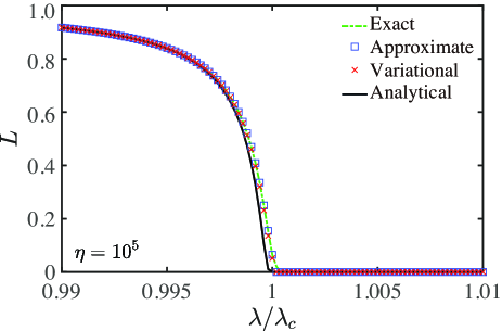
Figure 5: (Color online) The LE of the auxiliary atom versus the scaled coupling strength $\lambda/\lambda_{c}$ at $\omega_{c}t=60$. These curves are plotted with different methods: the numerical result based on the effective Hamiltonians given by Eqs. (18) and (34) (squares), the numerical result based on the original Rabi Hamiltonian given by Eq. (1) in the normal phase and Eq. (26) in the superradiance phase (green dashed line), and the variational method (crosses) for $\eta=10^{5}$. We also present the analytical result in the infinite $\eta$ case for reference (black solid line). Other parameters used are the same as those given in Fig. 3.

V SUMMARY

In summary, we have studied the dynamic sensitivity of quantum phase transition in the QRM by checking the LE of an auxiliary atom, which is far-off-resonantly coupled to the cavity field of the QRM. In the vicinity of the critical point, the LE displays a sudden decay, which is associated with the quantum decoherence of the auxiliary atom. We have checked quantum criticality of the QRM in both the infinite and finite $\eta$ cases. The analytical results in the infinite $\eta$ case clearly indicate the dynamic sensitivity in this model. Moreover, when the ratio $\eta$ between the frequency of the two-level atom and frequency of the cavity field is finite but large, i.e., in the finite $\eta$ case, the effective Hamiltonian can also reflect the quantum criticality in the QRM. Our proposal provides a simple scheme for observation of quantum criticality in the QRM by checking the quantum coherence of an atomic sensor.