Control-Data Separation and Logical Condition Propagation for Efficient Inference on Probabilistic Programs

Abstract

We present a novel sampling framework for probabilistic programs. The framework combines two recent ideas—control-data separation and logical condition propagation—in a nontrivial manner so that the two ideas boost the benefits of each other. We implemented our algorithm on top of Anglican. The experimental results demonstrate our algorithm’s efficiency, especially for programs with while loops and rare observations.

numbersnone#1none:
left:
right:

[nii]organization=National Institute of Informatics,addressline=Hitotsubashi 2-1-2, city=Chiyoda, postcode=101-8430, state=Tokyo, country=Japan

[sokendai]organization=Department of Informatics, SOKENDAI (The Graduate University for Advanced Studies),addressline=Shonan Village, city=Hayama, postcode=240-0193, state=Kanagawa, country=Japan

[ey]organization=Ernst & Young ShinNihon LLC,addressline=Yurakucho 1-1-2, city=Chiyoda, postcode=100-0006, state=Tokyo, country=Japan

[kyoto]organization=Graduate School of Informatics, Kyoto University,addressline=Yoshida-Honmachi 36-1, city=Kyoto, postcode=606-8501, state=Kyoto, country=Japan

To Luis Barbosa on the occasion of his sixtieth birthday. Luis’s works have always been inspirations and encouragements for us, showing the remarkable power of logic in various applications, such as reactive systems, cyber-physical systems, quantum systems, and data governance. The current work follows this spirit, demonstrating the power of (program) logic in statistics.

1 Introduction

Probabilistic Programs

In the recent rise of statistical machine learning, probabilistic programming languages are attracting a lot attention as a programming infrastructure for data processing tasks. Probabilistic programming frameworks allow users to express statistical models as programs, and offer a variety of methods for analyzing the models.

Probabilistic programs feature randomization and conditioning. Randomization can take different forms, such as probabilistic branching ($\mathtt{ifp}$ in Program 1) and random assignment from a probability distribution (denoted by $\sim$, see Program 2).

Conditioning—also called observation and evidence—makes the operational meaning of probabilistic programs unique and distinct from usual programs. Here, the meaning of “execution” is blurry since some execution traces get discarded due to observation violation. For example, in Line 8 of Program 1, we have $(c1,c2)=(\mathtt{true},\mathtt{true})$ with probability $0.36^{2}$; such an execution violates the observation !(c1 = c2) in Line 8 and is thus discarded.

It is suitable to think of a probabilistic programming language as a modeling language: a probabilistic program is not executed but is inferred on. Specifically, the randomization constructs in a program define the prior distribution; it is transformed by other commands such as deterministic assignment; and the semantics of the program is the posterior distribution, conditioned by the observation commands therein. This Bayesian view makes probabilistic programming a useful infrastructure for various statistical inference tasks. It poses a challenge to the programming language community, too, namely to come up with statistical inference techniques that are efficient, generic, and language-based.

Prog.  1: coin

⬇

bool c1, c2 := true;

ifp (0.36)

then c1 := true;

else c1 := false;

ifp (0.36)

then c2 := true;

else c2 := false;

observe(!(c1 = c2));

return(c1);

Prog.  2: obsLoop

⬇

1 double x := 0;

2 double y := 0;

3 int n := 0;

4 while (x < 3) {

5 n := n + 1;

6 y $\sim$ normal(1,1);

7 observe(0 <= y <= 2);

8 x := x + y;}

9 observe(n >= 5);

10 return(n);

The community’s efforts have produced a number of languages and inference frameworks. Many of them are sampling-based (as opposed to symbolic and exact): Anglican [1], Venture [2], Stan [3], and Pyro [4]. Recent topics include easing description of inference algorithms [5], assistance by DNNs [6], and proximity to general-purpose languages [7].

Challenges in Inference on Probabilistic Programs

In this paper, we pursue sampling-based approximate inference of probabilistic programs. In doing so, we encounter the following two major challenges.

The first is weight collapse, a challenge widely known in the community (see e.g. [Tsay18]). In sampling a statistical model, one typically sweeps it with a number of particles (i.e. potential samples). However, in case the model imposes rare observations, the particles’ weights quickly decay to zero, making the effective sample number tiny. Study of weight collapse has resulted in a number of advanced sampling methods. They include sequential Monte Carlo (SMC) featuring resampling, and Markov chain Monte Carlo (MCMC).

The second challenge, specific to probabilistic programs, is the compatibility between advanced sampling methods (such as SMC and MCMC) and control structures of probabilistic programs. There are a number of sampling anomalies resulting from control structures (see e.g. [HurNRS15]): MCMC walks often find difficulties in traversing different control flows; for gradient-based sampling methods (such as Hamiltonian MC and variational inference), discontinuities due to different control flows emerge as a major burden. See [Kiselyov16, ZhouYTR20] and [DBLP:journals/corr/abs-1809-10756, Section 3.4.2] for further discussions.

Figure 1: our hierarchical sampling architecture. It features control-data separation and logical condition propagation

Proposed Sampling Framework: Combining Two Ideas

In order to alleviate the above two challenges (weight collapse and compatibility between sampling and control), this paper proposes a hierarchical sampling framework shown in Figure 1. It combines two recent ideas for efficient inference on probabilistic programs, namely control-data separation [ZhouYTR20] and logical condition propagation [NoriHRS14]. We combine the two ideas in a nontrivial manner so that they boost each other’s benefits.

Idea 1: Hierarchical Sampler via Control-Data Separation

One feature of the proposed framework is the separation of control flow sampling and data sampling. In Figure 1, the top level sampler chooses a specific control flow $\vec{l}$, which is passed to the bottom level data sampler. The data sampler then focuses on the straight-line program that arises from the control flow $\vec{l}$; it is thus freed from the duty of dealing with control flows such as if branches and while loops.

In our framework, the top-level sampling is identified as what we call the infinite-armed sampling problem: from a (potentially infinite) set of control flows, we aim to draw samples according to their likelihoods, but the likelihoods are unknown and we learn them as the sampling goes on. This problem is a variation of the classic problem of multi-armed bandit (MAB), with the differences that 1) we sample rather than optimize, and 2) we have potentially infinitely many arms. We show how the well-known $\varepsilon$-greedy algorithm for MAB can be adapted for our purpose.

The bottom-level data sampling can be by various algorithms. We use SMC in this paper. This is because SMC—much like other importance sampling and particle filter methods, but unlike MCMC—can estimate the likelihood of a control flow $\vec{l}$ via the average weight of particles. This estimated likelihood is used in the top-level flow sampling (Figure 1). See Section 3.2.1 for discussion. Use of other algorithms for the bottom-level data sampling is future work. We expect that the control-data separation will ease the use of gradient-based algorithms (such as Hamiltonian MC and variational inference), since often each control flow denotes a differentiable function.

The idea of control-data separation appears in the recent work [ZhouYTR20], where it is pursued under the slogan “divide, conquer, and combine.” Our hierarchical framework (Figure 1) has a lot in common with the one in the work. At the same time, our framework—we started its development before the publication of [ZhouYTR20]—is designed as a language-based and static analysis-oriented realization of the idea of control-data separation. This is in contrast with [ZhouYTR20] that takes an alternative, more statistics-oriented approach (see [ZhouYTR20, Section 6.2]).

As shown in Figure 1, the two levels of sampling are interleaved in our framework, accumulating data samples in each iteration of the bottom-level sampling. Those data samples are suitably weighted so that the resulting data samples are unbiased. We note that our hierarchical framework does not aim to make the sampled distribution smooth—usually a probabilistic program does denote a distribution that is not smooth. Instead, it tries to make the most of partial smoothness that is inherent in the target probabilistic program, by letting a data sampling algorithm focus on a single control flow which is more likely to be smooth within.

Specifically, major differences between [ZhouYTR20] and ours are in 1) how we find new control flows (Remark 11); 2) how control flows are sampled (Remark 19); and, most notably, 3) the use of logical condition propagation (below).

Idea 2: Logical Condition Propagation, Domain Restriction, and Blacklisting

In this paper, we find an advantage of control-data separation in easing the application of logical reasoning for sampling efficiency. Specifically, we combine condition propagation—an idea originally introduced in R2 [NoriHRS14]—in the hierarchical framework in Figure 1. It logically propagates observations upwards in a program, so that sample rejection happens earlier and unnecessary samples are spared.

Condition propagation is much like a weakest precondition calculus, a well-known technique in program verification (see e.g. [Winskel93]). The original condition propagation in R2 is targeted at arbitrary programs, and this resulted in limited applicability. For example, it requires explicit loop invariants for condition propagation over while loops, but loop invariants are hard to find. In contrast, in our framework (Figure 1), condition propagation is only applied to straight-line programs (without if branchings or while loops), making the application of condition propagation easier and more robust.

We also introduce two important derivatives of condition propagation. One is domain restriction (Section 2.5): we restrict the domain of distributions to sample from, using the conditions obtained by condition propagation. The resulting distribution prohibits samples that will anyway be rejected.

The other is logical blacklisting of control flows (Section 3.2). Condition propagation often reveals that a control flow $\vec{l}$ is logically infeasible and thus has zero likelihood. This information is passed upwards in Figure 1, and we blacklist the flow $\vec{l}$ in the henceforth sampling. This use of condition propagation is unique to its combination with control-data separation (Figure 1); its effect is experimentally verified in Section 4.

There are other probabilistic programming frameworks that use static analysis. For example, Gen [DBLP:conf/pldi/Cusumano-Towner19] applies static analysis to its fragment called the static modeling language; Birch [MURRAY201829] uses static reasoning to delay sampling and enable analytical optimizations. The difference is that their use of static analysis is essentially limited to straight-line programs, which is in contrast with the current work where condition propagation applies to every program via control-data separation.

In [OlmedoGJKKM18] a program transformation called hoisting is introduced. Inspired by R2 [NoriHRS14], the transformation eliminates all observation commands in a program by propagating them backwards. Such elimination of observations is possible in [OlmedoGJKKM18] since their target language has randomization only in the form of probabilistic branching (such as $\{x\coloneqq 0\}[1/2]\{x\coloneqq 1\}$ for a fair coin). While probabilistic assignments from discrete distributions may be emulated by probabilistic branching, the language in [OlmedoGJKKM18] does not allow probabilistic assignments from continuous distributions, such as y $\sim$ normal(1,1) in Program 2. Due to the presence of the latter, our condition propagation does not totally eliminate observations in general.

Contributions and Organization

Our main contribution is a hierarchical sampling algorithm (Figure 1) that combines the ideas of control-data separation (one used in [ZhouYTR20]) and condition propagation [NoriHRS14]. It is mathematically derived in Section 3. This is preceded by Section 2, where we introduce the syntax and the semantics of our target language pIMP, as well as condition propagation.

Our other theoretical contributions include the formulation of the infinite-armed sampling (IAS) problem, its $\varepsilon$-greedy algorithm, and a convergence proof for the algorithm (restricting to finite arms, Section 3.1). Our hierarchical sampler is introduced as a refinement of this IAS algorithm (Section 3.2).

Our implementation is built on top of Anglican [TolpinMYW16] and is called Schism. In our experimental comparison with Anglican in Section 4, we witness Schism’s performance advantages, especially with programs with while loops and rare observations. We discuss potential application in the domain of testing automotive systems.

Many details are deferred to the appendix.

Notations

The sets of real numbers and nonnegative reals are ${\mathbb{R}}$ and ${\mathbb{R}_{\geq 0}}$, respectively. We write $x_{1:N}$ for a sequence $x_{1},x_{2},\dotsc,x_{N}$.

We use the following notation for Lebesgue integrals. Let $(X,\mu)$ be a measure space, and $f\colon X\to{\mathbb{R}}$ be a measurable function. We write

$$\textstyle\int_{x\in X}f(x)\,\mu(\mathrm{d}x)$$ (1)

for the integration of $f$ over $(X,\mu)$. This is almost the standard notation $\int_{X}f(x)\,\mu(\mathrm{d}x)$, where $\mathrm{d}x$ is understood as a measurable subset around $x$ (thus $x$ and $\mathrm{d}x$ are tied with each other). In our notation (1), we write $x\in X$ to make it explicit that $x$ is a bound variable that ranges over $X$.

This notation is extended as follows, which might be found a bit more unconventional. When the measure space in question is of the form $(Y\times Z,\mu)$, we write

$$\textstyle\int_{y\in Y,z\in Z}f(y,z)\,\mu(\mathrm{d}y\times\mathrm{d}z)$$

for the integration. Note here that the rectangles $\mathrm{d}y\times\mathrm{d}z$ generate the $\sigma$-algebra of the product measurable space $Y\times Z$.

2 The Language pIMP and pCFGs

2.1 Probabilistic Programming Language pIMP

We use an imperative probabilistic programming language whose syntax (Figure 2) closely follows [GordonHNR14]. The language is called pIMP; Program 1 & 2 are examples. pIMP features the following probabilistic constructs.

The probabilistic assignment command $x\sim\mathbf{Dist}(\vec{e})$ samples a value from the designated distribution and assigns it to the variable $x$. Here $\mathbf{Dist}$ specifies a family of probability distributions (such as normal, Bernoulli, etc.; they can be discrete or continuous), and $\vec{e}$ is a vector of parameters for the family $\mathbf{Dist}$, given by expressions for real numbers. An example is $x\sim\mathtt{normal}(0,1)$.

The probabilistic branching $\mathtt{ifp}\;p\;\mathtt{then}\;c_{1}\;\mathtt{else}\;c_{2}$ chooses one from $c_{1}$ and $c_{2}$ with the probabilities $p\in[0,1]$ and $1-p$, respectively. We introduce this as a shorthand for $b\sim\mathtt{Bernoulli}(p);\mathtt{if}\;b\;\mathtt{then}\;c_{1}\;\mathtt{else}\;c_{2}$, where $b$ is a fresh Boolean variable.

The soft conditioning command $\mathtt{weight}\;f$ is a primitive in pIMP, as is common in probabilistic programming languages. Here, $f$ is a fuzzy predicate—a function that returns a nonnegative real number—that tells how much weight the current execution should acquire.

We also use sharp conditioning $\mathtt{observe}\;\varphi$—where $\varphi$ is a Boolean formula rather than a fuzzy predicate—in our examples (see e.g. Program 1 & 2). This is a shorthand for $\mathtt{weight}\;\mathbf{1}_{\varphi}$, where $\mathbf{1}_{\varphi}$ is the characteristic function of the formula $\varphi$ ($\mathbf{1}_{\varphi}$ returns $1$ if $\varphi$ is true, and $0$ if $\varphi$ is false).

As usual, in Figure 2, only (sharp) Boolean formulas $\varphi$ are allowed as guards of if branchings and while loops.

$\begin{array}[]{lcllll}&x&\in&\mathbf{Var}\\ &\mathbf{c}&::=&\lx@intercol\text{constants, e.g.\ $0$, $-1.2$ and $\mathtt{true}$}\hfil\lx@intercol\\ &\mathop{\mathbf{uop}}&::=&\lx@intercol\parbox[t]{173.44534pt}{ unary operators, e.g.\ ``$-$'' in $-3$ }\hfil\lx@intercol\\ &\mathbin{\mathbf{bop}}&::=&\lx@intercol\parbox[t]{173.44534pt}{binary operations, e.g.\ $+$, $\&\&$}\hfil\lx@intercol\\ &\varphi&::=&\lx@intercol\text{Boolean formulas}\hfil\lx@intercol\\ &f&::=&\lx@intercol\parbox[t]{173.44534pt}{ fuzzy predicates, i.e.\\ \ expressions that return nonnegative real values }\hfil\lx@intercol\\[5.0pt] &e&::=&x\mid\mathbf{c}\mid e_{1}\mathbin{\mathbin{\mathbf{bop}}}e_{2}\mid\mathop{\mathbf{uop}}e&\\ &&&\lx@intercol\parbox[t]{130.08731pt}{value expressions\\ ($\mathtt{int}$, $\mathtt{bool}$, $\mathtt{double}$, etc.)}\hfil\lx@intercol\end{array}\begin{array}[]{lcllll}&c&::=&&\text{commands}\\ &&&\mathtt{skip}&\text{skip}\\ &&&\mid x:=e&\text{deterministic assignment}\\ &&&\mid x\sim\mathbf{Dist}(\vec{e})&\text{probabilistic assignment}\\ &&&\mid\mathtt{weight}\;f&\parbox[t]{130.08731pt}{soft conditioning by a fuzzy predicate}\\ &&&\mid c_{1};\,c_{2}&\text{sequential composition}\\ &&&\mid\mathtt{if}\;\varphi\;\mathtt{then}\;c_{1}\;\mathtt{else}\;c_{2}&\text{conditional branching}\\ &&&\mid\mathtt{while}(\varphi)\{c\}&\text{while loop}\\[6.99997pt] &\pi&::=&c\,;\;\mathtt{return}\;e&\text{program}\end{array}$

Figure 2: the probabilistic programming language pIMP, syntax. The set $\mathbf{Var}$ of variables is fixed. The $\mathtt{ifp}$ construct in Program 1 is a shorthand; see Section 2.1.

2.2 Probabilistic Control Flow Graphs (pCFGs)

We use the notion of probabilistic control flow graph (pCFG), adapted from [AgrawalCN18], for presenting pIMP programs as graphs. It is a natural probabilistic variation of control flow graphs for imperative programs.

Figure 3: pCFG for obsLoop (Program 2).

A pCFG is a finite graph, its nodes roughly correspond to lines of a pIMP program, and its edges have transition labels that correspond to atomic commands of pIMP. An example is in Figure 3: $l_{\mathrm{init}}$ is the initial location; the label into $l_{\mathrm{init}}$ specifies the initial memory state $\sigma_{\mathrm{init}}$; $l_{\mathrm{final}}$ is the final location; and the label out of $l_{\mathrm{final}}$ ($n$ here) specifies the return expression $e_{\mathrm{final}}$.

Our formal definition (Definition 1) differs from [AgrawalCN18] mainly in the following: 1) presence of weight commands; and 2) absence of nondeterminism.

Definition 1 (pCFG, adapted from [AgrawalCN18]).

A probabilistic control flow graph (pCFG) is a tuple $\Gamma=(L,V,l_{\mathrm{init}},\sigma_{\mathrm{init}},l_{\mathrm{final}},e_{\mathrm{final}},\rightarrow,\lambda)$ that consists of the following components.

• A finite set $L$ of locations, equipped with a partition $L=L_{\mathsf{D}}+L_{\mathsf{PA}}+L_{\mathsf{DA}}+L_{\mathsf{W}}+\{l_{\mathrm{final}}\}$ into deterministic, probabilistic assignment, deterministic assignment, weight and final locations.

• A finite set $V=\{x_{1},\ldots,x_{|V|}\}$ of program variables. It is a subset of the set $\mathbf{Var}$ of variables.

• An initial location $l_{\mathrm{init}}\in L$, and an initial memory state $\sigma_{\mathrm{init}}\colon V\to{\mathbb{R}}$.

• A final location $l_{\mathrm{final}}\in L$, and a return expression $e_{\mathrm{final}}$.

• A transition relation ${\rightarrow}\subseteq L\times L$.

• A labeling function $\lambda$.

A labeling function $\lambda$ assigns to each transition $l\to l^{\prime}$ a command, a formula or a real number. It is subject to the following conditions.

• Each deterministic location $l\in L_{\mathsf{D}}$ has two outgoing transitions. One is labeled with a (sharp) Boolean formula $\varphi$; the other is labeled with its negation $\mathop{!}\varphi$.

• Each probabilistic assignment location $l\in L_{\mathsf{PA}}$ has one outgoing transition. It is labeled with a probabilistic assignment command $x\sim\mathbf{Dist}(\vec{e})$.

• Each deterministic assignment location $l\in L_{\mathsf{DA}}$ has one outgoing transition. It is labeled with a deterministic assignment command $x\coloneqq e$.

• Each weight location $l\in L_{\mathsf{W}}$ has one outgoing transition, labeled with a command $\mathtt{weight}\;f$. We also use $\mathtt{observe}\;\varphi$ as a label from time to time. Recall that $\mathtt{observe}\;\varphi$ is a shorthand for $\mathtt{weight}\;\mathbf{1}_{\varphi}$, where $\mathbf{1}_{\varphi}$ is the characteristic function for the Boolean formula $\varphi$.

• The final location $l_{\mathrm{final}}$ has no successor with respect to $\to$.

In the last definition, we assume that the values of all the basic types ($\mathtt{int}$, $\mathtt{bool}$, $\mathtt{double}$, etc.) are embedded in ${\mathbb{R}}$. Using different value domains is straightforward but cumbersome.

(a) A deterministic location $l\in L_{\mathsf{D}}$.

(b) A probabilistic assignment location $l\in L_{\mathsf{PA}}$.

(c) A deterministic assignment location $l\in L_{\mathsf{DA}}$.

(d) A weight location $l\in L_{\mathsf{W}}$.

Figure 4: pCFG locations

Figure 4 illustrates the five types of pCFG locations.

The translation from pIMP programs to pCFGs is straightforward, following [AgrawalCN18]; its details are thus omitted.

2.3 Semantics of pCFGs

We introduce formal semantics of pCFGs in a denotational style; see [Winskel93] for basics. We need semantics to formulate soundness of condition propagation (Section 2.5); we also use the semantics in the description of our sampling algorithm. We follow [StatonYWHK16]—which is inspired ultimately by [Kozen81]—and introduce the following two semantics:

• The weighted state transformer semantics $\llbracket\underline{\phantom{n}}\,\rrbracket^{\mathsf{w\text{-}st}}$ (Definition 4), where weights from soft conditioning are recorded by the weights of samples.

• The (unweighted, normalized) state transformer semantics $\llbracket\underline{\phantom{n}}\,\rrbracket^{\mathsf{st}}$ (Definition 5), obtained by normalizing the weighted semantics $\llbracket\underline{\phantom{n}}\,\rrbracket^{\mathsf{w\text{-}st}}$. In particular, the normalization process removes samples of weight $0$, i.e. those which violate observations. This is the semantics we wish to sample from.

These semantics are defined in terms of memory states (assignments of values to variables). The actual definition is by induction on the construction of programs, exploiting the $\omega$-cpo structure of $\mathcal{D}_{\leq 1}X$, the set of subprobability distributions. An example is given later (Example 6).

Definition 2.

Let $X$ be a measurable space. The set of probability distributions over $X$ is denoted by $\mathcal{D}(X)$. The set of subprobability distributions $\mu$ over $X$—for which $\mu(X)$ is required to be $\leq 1$ rather than $=1$—is denoted by $\mathcal{D}_{\leq 1}(X)$. We equip both $\mathcal{D}(X)$ and $\mathcal{D}_{\leq 1}(X)$ with suitable $\sigma$-algebras given by [Giry82].

The set $\mathcal{D}_{\leq 1}(X)$ comes with a natural order $\leq$ defined as follows: $\mu\leq\nu$ if $\mu(U)\leq\nu(U)$ (in ${\mathbb{R}}$) for each measurable subset $U$. The set $\mathcal{D}_{\leq 1}(X)$ is an $\omega$-cpo with respect to $\leq$; its bottom element is given by the zero distribution (assigning $0$ to every measurable subset). The $\omega$-cpo structure is inherited by function spaces of the form $(\mathcal{D}_{\leq 1}(X))^{A}$, where $A$ is an arbitrary set, where the order is defined pointwise. Note that this order becomes trivial in $\mathcal{D}(X)$ due to the normalization condition.

For a distribution $\mu$, its support is denoted by $\mathsf{supp}(\mu)$. The Dirac distribution at $x\in X$ is denoted by $\delta_{x}$.

Definition 3 (memory state, interpretation of expressions).

Let $\Gamma=(L,V,\dotsc)$ be a pCFG. A memory state $\sigma$ for $\Gamma$ is a function $\sigma\colon V\to{\mathbb{R}}$ that maps each variable $x\in V$ to its value $\sigma(x)$. (Recall from Section 2 that, for simplicity, we embed the values of all basic types in ${\mathbb{R}}$.) The interpretation $\llbracket e\rrbracket_{\sigma}$ of an expression $e$ under $\sigma$ is defined inductively; so is the interpretation $\llbracket\varphi\rrbracket_{\sigma}$ of a Boolean formula.

We define $\mathbf{St}$ to be the measurable space over the set of functions of type $V\to{\mathbb{R}}$, equipped with the coarsest $\sigma$-algebra making the evaluation function $(\underline{\phantom{n}}\,)(x):(V\to{\mathbb{R}})\to{\mathbb{R}}$ measurable for each $x\in V$. This makes $\mathbf{St}$ isomorphic to the product of $|V|$-many copies of ${\mathbb{R}}$.

Definition 4 (weighted state transformer semantics $\llbracket\underline{\phantom{n}}\,\rrbracket^{\mathsf{w\text{-}st}}$).

Let $\Gamma=(L,V,l_{\mathrm{init}},\sigma_{\mathrm{init}},l_{\mathrm{final}},e_{\mathrm{final}},\rightarrow,\lambda)$ be a pCFG. For each location $l\in L$ of the pCFG $\Gamma$, we define its interpretation

$$\llbracket\Gamma,l\rrbracket^{\mathsf{w\text{-}st}}\colon\mathbf{St}\longrightarrow\mathcal{D}_{\leq 1}\bigl{(}{\mathbb{R}_{\geq 0}}\times\mathbf{St}\bigr{)},$$

which is a measurable function, by the least solution of the system of recursive equations shown in Figure 5. Intuitively, $\llbracket\Gamma,l\rrbracket^{\mathsf{w\text{-}st}}(\sigma)$ is the subprobability distribution of weighted samples of memory states, obtained at the final state $l_{\mathrm{final}}$ after an execution of $\Gamma$ that starts at the location $l$ with a memory state $\sigma$. It is a sub-probability distribution since an execution might be nonterminating.

For the whole pCFG $\Gamma$, its weighted state transformer semantics

$$\llbracket\Gamma\rrbracket^{\mathsf{w\text{-}st}}\in\mathcal{D}_{\leq 1}\bigl{(}{\mathbb{R}_{\geq 0}}\times{\mathbb{R}}\bigr{)}$$ (2)

is defined as follows, using an intermediate construct $\llbracket\Gamma\rrbracket^{\overline{\mathsf{w\text{-}st}}}\in\mathcal{D}_{\leq 1}\bigl{(}{\mathbb{R}_{\geq 0}}\times\mathbf{St}\bigr{)}$.

$$\llbracket\Gamma\rrbracket^{\overline{\mathsf{w\text{-}st}}}\;\coloneqq\;\llbracket\Gamma,l_{\mathrm{init}}\rrbracket^{\mathsf{w\text{-}st}}(\sigma_{\mathrm{init}}),$$

$$\llbracket\Gamma\rrbracket^{\mathsf{w\text{-}st}}(\mathrm{d}w\times\mathrm{d}v)\;\coloneqq\;\int_{\sigma\in\mathbf{St}}\delta_{\llbracket e_{\mathrm{final}}\rrbracket_{\sigma}}(\mathrm{d}v)\,\cdot\,\llbracket\Gamma\rrbracket^{\overline{\mathsf{w\text{-}st}}}(\mathrm{d}w\times\mathrm{d}\sigma)\enspace.$$ (3)

Recall that $\delta_{\llbracket e_{\mathrm{final}}\rrbracket_{\sigma}}$ is a Dirac distribution: $\delta_{\llbracket e_{\mathrm{final}}\rrbracket_{\sigma}}(\mathrm{d}v)=1$ if and only if $\llbracket e_{\mathrm{final}}\rrbracket_{\sigma}\in\mathrm{d}v$; its value is $0$ otherwise.

$$\llbracket\Gamma,l\rrbracket^{\mathsf{w\text{-}st}}(\sigma) =\begin{cases}\llbracket\Gamma,l^{\prime}\rrbracket^{\mathsf{w\text{-}st}}(\sigma)&\text{if $\llbracket\varphi\rrbracket_{\sigma}=\mathtt{true}$}\\ \llbracket\Gamma,l^{\prime\prime}\rrbracket^{\mathsf{w\text{-}st}}(\sigma)&\text{if $\llbracket\varphi\rrbracket_{\sigma}=\mathtt{false}$}\end{cases}$$

$$\llbracket\Gamma,l\rrbracket^{\mathsf{w\text{-}st}}(\sigma) =\int_{v\in{\mathbb{R}}}\llbracket\Gamma,l^{\prime}\rrbracket^{\mathsf{w\text{-}st}}\bigl{(}\sigma[x\mapsto v]\bigr{)}\cdot\mathbf{Dist}\bigl{(}\llbracket\vec{e}\rrbracket_{\sigma}\bigr{)}(v)\;\mathrm{d}v$$

$$\llbracket\Gamma,l\rrbracket^{\mathsf{w\text{-}st}}(\sigma) =\llbracket\Gamma,l^{\prime}\rrbracket^{\mathsf{w\text{-}st}}\bigl{(}\,\sigma\bigl{[}x\mapsto\llbracket e\rrbracket_{\sigma}\bigr{]}\,\bigr{)}$$

$$\llbracket\Gamma,l\rrbracket^{\mathsf{w\text{-}st}}(\sigma) =\begin{cases}\boldsymbol{\lambda}(\mathrm{d}r\times\mathrm{d}\sigma^{\prime}).\;\llbracket f\rrbracket_{\sigma}\cdot\llbracket\Gamma,l^{\prime}\rrbracket^{\mathsf{w\text{-}st}}(\sigma)\bigl{(}(\mathrm{d}r/\llbracket f\rrbracket_{\sigma})\times\mathrm{d}\sigma^{\prime}\bigr{)}\\ \qquad\qquad\qquad\qquad\text{if $\llbracket f\rrbracket_{\sigma}\neq 0$;}\\ \boldsymbol{\lambda}(\mathrm{d}r\times\mathrm{d}\sigma^{\prime}).\;\\ \qquad\begin{cases}\int_{r^{\prime}\in{\mathbb{R}_{\geq 0}}}\llbracket\Gamma,l^{\prime}\rrbracket^{\mathsf{w\text{-}st}}(\sigma)(\mathrm{d}r^{\prime}\times\mathrm{d}\sigma^{\prime})\\ \phantom{0}\qquad\text{if $0\in\mathrm{d}r$;}\\ 0\qquad\text{otherwise;}\end{cases}\\ \qquad\qquad\qquad\qquad\text{if $\llbracket f\rrbracket_{\sigma}=0$}\end{cases}$$ (4)

$$\llbracket\Gamma,l_{\mathrm{final}}\rrbracket^{\mathsf{w\text{-}st}}(\sigma) =\delta_{(1,\sigma)}$$

Figure 5: Recursive definition of $\llbracket\Gamma,l\rrbracket^{\mathsf{w\text{-}st}}$ used in the weighted state transformer semantics of pCFGs

Intuitively, the definition (3) is the continuous variation of the following one (that only makes sense if all the value domains are discrete).

$$\llbracket\Gamma\rrbracket^{\mathsf{w\text{-}st}}(w,v)\;\coloneqq\;\sum_{\sigma\text{ s.t.\ }\llbracket e_{\mathrm{final}}\rrbracket_{\sigma}=v}\llbracket\Gamma,l_{\mathrm{init}}\rrbracket^{\mathsf{w\text{-}st}}(\sigma_{\mathrm{init}})(w,\sigma)\enspace.$$

Similarly, the case (4) for $\mathtt{weight}$ locations in Figure 5 can be described more simply if the distributions involved are discrete. Let the distribution $\llbracket\Gamma,l^{\prime}\rrbracket^{\mathsf{w\text{-}st}}(\sigma)$ be $\bigl{[}\,(r_{i},\sigma^{\prime}_{i})\mapsto p_{i}\,\bigr{]}_{i}$, where each pair $(r_{i},\sigma^{\prime}_{i})$ of a weight and a state gets a probability $p_{i}$ assigned. Then the distribution $\llbracket\Gamma,l\rrbracket^{\mathsf{w\text{-}st}}(\sigma)$ should be given by $\bigl{[}\,\bigl{(}\,\llbracket f\rrbracket_{\sigma}\cdot r_{i},\,\sigma^{\prime}_{i}\,\bigr{)}\mapsto p_{i}\,\bigr{]}_{i}$, where we multiply all the weights $r_{i}$ by the nonnegative real number $\llbracket f\rrbracket_{\sigma}$. In particular, if $\llbracket f\rrbracket_{\sigma}=0$, then we should have

$$\bigl{(}\,\llbracket\Gamma,l\rrbracket^{\mathsf{w\text{-}st}}(\sigma)\,\bigr{)}(0,\sigma^{\prime}) =\textstyle\sum_{r^{\prime}\in{\mathbb{R}_{\geq 0}}}\bigl{(}\,\llbracket\Gamma,l^{\prime}\rrbracket^{\mathsf{w\text{-}st}}(\sigma)\,\bigr{)}(r^{\prime},\sigma^{\prime})\enspace,$$ (5)

$$\bigl{(}\,\llbracket\Gamma,l\rrbracket^{\mathsf{w\text{-}st}}(\sigma)\,\bigr{)}(r,\sigma^{\prime}) =0\qquad\text{if $r>0$.}$$

Based on the last intuition, the full definition (4) in Figure 5 is explained as follows. In the first line, $\mathrm{d}r/\llbracket f\rrbracket_{\sigma}$ denotes the measurable set $\mathrm{d}r$ scaled by $1/\llbracket f\rrbracket_{\sigma}$; for example, if $\mathrm{d}r=[s,t]$, then $\mathrm{d}r/\llbracket f\rrbracket_{\sigma}=\bigl{[}s/\llbracket f\rrbracket_{\sigma},t/\llbracket f\rrbracket_{\sigma}\bigr{]}$. This achieves the effect of “multiplying weights $r_{i}$ by $\llbracket f\rrbracket_{\sigma}$,” with the side-effect, however, of changing the measure of the set $\mathrm{d}r$. The first occurrence of $\llbracket f\rrbracket_{\sigma}$ in the first line of (4) cancels this side-effect. The second case of (4) in Figure 5 (Lines 3–7) is a continuous adaptation of (5).

The least solution of the recursive equation for $\bigl{(}\llbracket\Gamma,l\rrbracket^{\mathsf{w\text{-}st}}\bigr{)}_{l\in L}$ in Figure 5 exists. It can be constructed as the supremum of a suitable increasing $\omega$-chain, exploiting the $\omega$-cpo structure of the set of measurable functions of type $\mathbf{St}\times L\to\mathcal{D}_{\leq 1}\bigl{(}{\mathbb{R}_{\geq 0}}\times\mathbf{St}\bigr{)}$. See e.g. [GordonHNR14].

This construction via a supremum also matches the operational intuition of collecting the return values of all the execution paths of length $0,1,2,\dotsc$.

The weighted semantics $\llbracket\Gamma\rrbracket^{\mathsf{w\text{-}st}}\in\mathcal{D}_{\leq 1}\bigl{(}{\mathbb{R}_{\geq 0}}\times{\mathbb{R}}\bigr{)}$ in (2) is randomized, since an execution of $\Gamma$ has uncertainties that come from the randomizing construct $x\sim\mathbf{Dist}(\vec{e})$. It is a subprobability distribution—meaning that the probabilities need not sum up to $1$, see Definition 2—since an execution of $\Gamma$ may not terminate. See e.g. [MorganMS96]. Note that violation of observations $\mathtt{observe}\;\varphi$ is recorded as the zero weight (in the ${\mathbb{R}_{\geq 0}}$ part in (2)), rather than making the sample disappear.

By applying normalization to the weighted semantics in Definition 4, we obtain the following (unweighted) state transformer semantics. This semantics is the posterior distribution in the sense of Bayesian inference. It is therefore the distribution that we would like to sample from.

Definition 5 ((unweighted) state transformer semantics $\llbracket\underline{\phantom{n}}\,\rrbracket^{\mathsf{st}}$).

Let $\Gamma$ be a pCFG. Its state transformer semantics is the probability distribution

$$\llbracket\Gamma\rrbracket^{\mathsf{st}}\in\mathcal{D}({\mathbb{R}})$$ (6)

defined as follows, using an intermediate construct $\llbracket\Gamma\rrbracket^{\overline{\mathsf{st}}}\in\mathcal{D}(\mathbf{St})$.

$$\llbracket\Gamma\rrbracket^{\overline{\mathsf{st}}}(\mathrm{d}\sigma)\coloneqq\frac{\int_{r\in{\mathbb{R}}}\,r\cdot\llbracket\Gamma\rrbracket^{\overline{\mathsf{w\text{-}st}}}(\mathrm{d}r\times\mathrm{d}\sigma)\,}{\int_{r\in{\mathbb{R}},\sigma^{\prime}\in\mathbf{St}}\,r\cdot\llbracket\Gamma\rrbracket^{\overline{\mathsf{w\text{-}st}}}(\mathrm{d}r\times\mathrm{d}\sigma^{\prime})}\enspace;$$ (7)

$$\llbracket\Gamma\rrbracket^{\mathsf{st}}(\mathrm{d}v)\coloneqq\textstyle\int_{\sigma\in\mathbf{St}}\,\delta_{\llbracket e_{\mathrm{final}}\rrbracket_{\sigma}}(\mathrm{d}v)\cdot\llbracket\Gamma\rrbracket^{\overline{\mathsf{st}}}(\mathrm{d}\sigma)\enspace.$$

Here $\delta_{\llbracket e_{\mathrm{final}}\rrbracket_{\sigma}}$ is the Dirac distribution at $\llbracket e_{\mathrm{final}}\rrbracket_{\sigma}$. The semantics is undefined in case the denominator $\int_{r\in{\mathbb{R}},\sigma^{\prime}\in\mathbf{St}}\,r\cdot\llbracket\Gamma\rrbracket^{\overline{\mathsf{w\text{-}st}}}(\mathrm{d}r\times\mathrm{d}\sigma^{\prime})$ is $0$.

Example 6.

The program coin in Program 1 emulates a fair coin using a biased one, crucially relying on the $\mathtt{observe}$ command (Line 1). Let $\Gamma$ be the pCFG induced by it. The return value domain is ${\mathbb{D}}=\mathbf{Bool}$.

The weighted semantics is $\llbracket\Gamma\rrbracket^{\mathsf{w\text{-}st}}=\bigl{[}(0,\mathtt{true})\mapsto 0.36^{2},(1,\mathtt{true})\mapsto 0.36\times 0.64,(1,\mathtt{false})\mapsto 0.64\times 0.36,(0,\mathtt{false})\mapsto 0.64^{2}\bigr{]}\in\mathcal{D}_{\leq 1}\bigl{(}{\mathbb{R}_{\geq 0}}\times\mathbf{Bool}\bigr{)}$. Here the first sample $(0,\mathtt{true})$—it comes from the memory state $[c1\mapsto\mathtt{true},c2\mapsto\mathtt{true}]$—has a weight $0$ due to its violation of the observation $\mathtt{!(c1=c2)}$. After normalization (which wipes out the contribution of the weighted sample $(0,\mathtt{true})$), we obtain the unweighted semantics $\llbracket\Gamma\rrbracket^{\mathsf{st}}=[\mathtt{true}\mapsto 1/2,\mathtt{false}\mapsto 1/2]$, as expected.

2.4 Control Flows and Straight-Line Programs

In our hierarchical architecture (Figure 1), the top-level chooses a complete control flow $\vec{l}$ of a pCFG; $\vec{l}$ induces a straight-line program $\mathrm{SLP}(\raisebox{0.0pt}[0.0pt][0.0pt]{$\vec{l}$})$; and the bottom-level data sampler works on $\mathrm{SLP}(\raisebox{0.0pt}[0.0pt][0.0pt]{$\vec{l}$})$. These notions are formally defined below; roughly, a control flow is a path in a pCFG that starts at the initial state $l_{\mathrm{init}}$; and a complete control flow is one that ends at the final location $l_{\mathrm{final}}$. In the definition of the straight-line program $\mathrm{SLP}(\raisebox{0.0pt}[0.0pt][0.0pt]{$\vec{l}$})$, the main point is to turn guards (for if branchings and while loops) into suitable observations.

Definition 7 (control flow).

Let $\Gamma=(L,V,l_{\mathrm{init}},\sigma_{\mathrm{init}},l_{\mathrm{final}},e_{\mathrm{final}},\rightarrow,\lambda)$ be a pCFG. A control flow of $\Gamma$ is a finite sequence $\raisebox{0.0pt}[0.0pt][0.0pt]{$\vec{l}$}=l_{1}l_{2}\dotsc l_{n}$ of locations, where we require $l_{1}=l_{\mathrm{init}}$ and $(l_{i},l_{i+1})\in{\to}$ for each $i\in[1,n-1]$. A control flow is often denoted together with transition labels, that is,

$$l_{\mathrm{init}}\;=\;l_{1}\xrightarrow{\lambda(l_{1},l_{2})}l_{2}\xrightarrow{\lambda(l_{2},l_{3})}\cdots\xrightarrow{\lambda(l_{n-1},l_{n})}l_{n}\enspace.$$

A control flow $\raisebox{0.0pt}[0.0pt][0.0pt]{$\vec{l}$}=l_{1}l_{2}\dotsc l_{n}$ is said to be complete if $l_{n}=l_{\mathrm{final}}$.

The set of control flows of a pCFG $\Gamma$ is denoted by $\mathbf{CF}(\Gamma)$; the set of complete ones is denoted by $\mathbf{CCF}(\Gamma)$.

Definition 8 (straight-line program).

A straight-line program is a pCFG that has no deterministic locations.

Therefore, a straight-line program is identified with a triple

$$\bigl{(}\,l_{\mathrm{init}}\xrightarrow{\lambda_{1}}l_{2}\xrightarrow{\lambda_{2}}\cdots\xrightarrow{\lambda_{n-1}}l_{\mathrm{final}},\;\,\sigma_{\mathrm{init}},\;\,e_{\mathrm{final}}\,\bigr{)}\enspace,$$

that shall be also denoted by

$$\xrightarrow{\sigma_{\mathrm{init}}}l_{\mathrm{init}}\xrightarrow{\lambda_{1}}l_{2}\xrightarrow{\lambda_{2}}\cdots\xrightarrow{\lambda_{n-1}}l_{\mathrm{final}}\xrightarrow{e_{\mathrm{final}}}\enspace.$$

The first component of the above triple is a chain that consists of the following types of locations: 1) assignment locations $l\xrightarrow{x\sim\mathbf{Dist}(\vec{e})}\cdot\,$ and $l\xrightarrow{x\coloneqq e}\cdot\,$; 2) weight locations $l\xrightarrow{\mathtt{weight}\;f}\cdot$ (where we might use $l\xrightarrow{\mathtt{observe}\;\varphi}\cdot$ as a shorthand); and 3) a final location. The remaining components are an initial memory state $\sigma_{\mathrm{init}}$ and a return expression $e_{\mathrm{final}}$.

Definition 9 (the straight-line program $\mathrm{SLP}(\raisebox{0.0pt}[0.0pt][0.0pt]{$\vec{l}$})$).

Let $\Gamma$ be a pCFG, and $\raisebox{0.0pt}[0.0pt][0.0pt]{$\vec{l}$}=l_{1}\dotsc l_{n}$ be a complete control flow of $\Gamma$. The straight-line program $\mathrm{SLP}(\raisebox{0.0pt}[0.0pt][0.0pt]{$\vec{l}$})$ is obtained by applying the following operation to $\raisebox{0.0pt}[0.0pt][0.0pt]{$\vec{l}$}=l_{1}\dotsc l_{n}$.

Each deterministic location $l_{i}\in L_{\mathsf{D}}$ occurring in $\vec{l}$ is changed into an observation location. Accordingly, the label of the transition $l_{i}\xrightarrow{\varphi}l_{i+1}$ is made into an observation command, resulting in $l_{i}\xrightarrow{\mathtt{observe}\;\varphi}l_{i+1}$.

Example 10 ($\mathrm{SLP}(\raisebox{0.0pt}[0.0pt][0.0pt]{$\vec{l}$})$).

For the pCFG in Figure 3, the set of complete control flows is $\{\raisebox{0.0pt}[0.0pt][0.0pt]{$\vec{l}$}_{n}\mid n\geq 0\}$ where $\raisebox{0.0pt}[0.0pt][0.0pt]{$\vec{l}$}_{n}\,:=\,l_{\mathrm{init}}\,\bigl{(}l^{(2)}l^{(3)}l^{(4)}l^{(5)}l_{\mathrm{init}}\bigr{)}^{n}\,l^{(6)}\,l_{\mathrm{final}}$. The flow $\raisebox{0.0pt}[0.0pt][0.0pt]{$\vec{l}$}_{1}$ induces the following straight-line program.

$$\small\begin{array}[]{l}\mathrm{SLP}(\raisebox{0.0pt}[0.0pt][0.0pt]{$\vec{l}$}_{1})=\left(\,\begin{array}[]{l}\xrightarrow{\sigma_{\mathrm{init}}}l_{\mathrm{init}}\xrightarrow{\mathtt{observe}\;x<3}l^{(2)}\xrightarrow{n:=n+1}l^{(3)}\\ \xrightarrow{y\sim\mathtt{normal}(1,1)}l^{(4)}\xrightarrow{\mathtt{observe}\;0\leq y\leq 2}l^{(5)}\xrightarrow{{\color[rgb]{0,0,0}x:=x+y}}l_{\mathrm{init}}\\ \xrightarrow{\mathtt{observe}\;\mathop{!}(x<3)}l^{(6)}\xrightarrow{{\color[rgb]{0,0,0}\mathtt{observe}\;n\geq 5}}\,l_{\mathrm{final}}\xrightarrow{n}\end{array}\,\right)\end{array}$$

Here $\sigma_{\mathrm{init}}=[\,x\mapsto 0,\,y\mapsto 0,\,n\mapsto 0]$. Note that the label $x<3$ going out of $l_{\mathrm{init}}$ in Figure 3 has been turned into the observation command $\mathtt{observe}\;x<3$ in $\mathrm{SLP}(\raisebox{0.0pt}[0.0pt][0.0pt]{$\vec{l}$}_{1})$.

We use a breadth-first search algorithm for the static discovery of control flows. A high-level description of the algorithm is as follows. A search tree $\mathcal{T}$ is obtained by (partially) unrolling the pCFG $\Gamma$. Additionally, each node $n$ of $\mathcal{T}$ records its distance from its shallowest descendant that is an open leaf (called the height of $n$). The search for a new control flow goes down from the root, choosing a child with the smallest height. When there are multiple such children, we pick one of them randomly.

While the algorithm is quite straightforward, we formally describe it in Algorithm 1 for the record. The algorithm uses the following notions. A search tree $\mathcal{T}$ for a pCFG $\Gamma=(L,V,l_{\mathrm{init}},\sigma_{\mathrm{init}},l_{\mathrm{final}},e_{\mathrm{final}},\rightarrow,\lambda)$ (as in Definition 1) is a finite tree with a branching degree $\leq 2$, identified as a subset $\mathcal{T}\subseteq\{0,1\}^{*}$ as usual. Each node $n$ of a search tree $\mathcal{T}$ is labeled with a location $\mathop{\mathrm{loc}}(n)\in L$ of $\Gamma$, and each edge of $\mathcal{T}$ is labeled in the same manner as with the labeling function $\lambda$ of $\Gamma$ (precisely, the edges from a node $n$ have the same labels as the edges from $\mathop{\mathrm{loc}}(n)$ in $\Gamma$). A node $n^{\prime}$ of $\mathcal{T}$ is an open leaf if it is a leaf in $\mathcal{T}$ and $\mathop{\mathrm{loc}}(n^{\prime})$ is not final ($\mathop{\mathrm{loc}}(n^{\prime})\neq l_{\mathrm{final}}$), in which case the control flow represented by $n^{\prime}$ is still incomplete. The height $0pt(n)$ of a node $n$ is the distance from its shallowest open leaf. Initially, a search tree $\mathcal{T}$ is set to be the one-node tree $\{\varepsilon\}$—where $\varepsilon$ represents the empty sequence, identified as the root—with $\mathop{\mathrm{loc}}(\varepsilon)=l_{\mathrm{init}}$ and $0pt(\varepsilon)=0$.

We do not use the usual queue-based implementation of breadth-first search. The reason is that the search tree $\mathcal{T}$ we explicitly construct in Algorithm 1 is a convenient data structure for sampling control flows (Algorithms 2 & 3).

Algorithm 1 Our static algorithm for control flow discovery by breadth-first search. It grows a search tree $\mathcal{T}$, potentially yielding a control flow 1:pCFG $\Gamma=(L,V,l_{\mathrm{init}},\sigma_{\mathrm{init}},l_{\mathrm{final}},e_{\mathrm{final}},\rightarrow,\lambda)$, search tree $\mathcal{T}$ with at least one open leaf (i.e. $0pt(\varepsilon)<\infty$) 2:search tree, control flow of $\Gamma$ 3:$\mathsf{cnode}\leftarrow\epsilon$ $\triangleright$ set the current node to the root 4:while $\mathsf{newCtrlFlow}$ is not defined do 5:    while $\mathsf{cnode}$ is not a leaf of $\mathcal{T}$ do $\triangleright$ search for a shallowest open leaf 6:        if $\mathop{\mathrm{loc}}(\mathsf{cnode})\in L_{\mathsf{PA}}\cup L_{\mathsf{DA}}\cup L_{\mathsf{W}}$ then $\triangleright$ $\mathsf{cnode}$ has only one child 7:           $\mathsf{cnode}\leftarrow\mathsf{cnode}\cdot 0$ 8:        else$\triangleright$ $\mathop{\mathrm{loc}}(\mathsf{cnode})\in L_{\mathsf{D}}$ and thus $\mathsf{cnode}$ has two children 9:           $\mathsf{cnode}\leftarrow\mathsf{cnode}\cdot\bigl{(}\,\operatorname*{arg\,min}_{i\in\{0,1\}}0pt(\mathsf{cnode}\cdot i)\,\bigr{)}$              10: 11:     add the children of $\mathsf{cnode}$ ($\mathsf{cnode}\cdot 0$ and $\mathsf{cnode}\cdot 1$ if $\mathop{\mathrm{loc}}(\mathsf{cnode})\in L_{\mathsf{D}}$, or only $\mathsf{cnode}\cdot 0$ otherwise) to $\mathcal{T}$ 12:$\triangleright$ now $\mathsf{cnode}$ is an open leaf by construction 13:     label the new children to define $\mathop{\mathrm{loc}}(\mathsf{cnode}\cdot 0)$ and $\mathop{\mathrm{loc}}(\mathsf{cnode}\cdot 1)$, using the successors of $\mathop{\mathrm{loc}}(\mathsf{cnode})$ in $\Gamma$ 14:    label the edges from $\mathsf{cnode}$ to its children accordingly 15:    for each child $\mathsf{cnode}\cdot i$ of $\mathsf{cnode}$ do 16:        if $\mathop{\mathrm{loc}}(\mathsf{cnode}\cdot i)=l_{\mathrm{final}}$ then 17:           $0pt(\mathsf{cnode}\cdot i)\leftarrow\infty$ 18:           $\mathsf{newCtrlFlow}\leftarrow\mathop{\mathrm{loc}}(\mathsf{cnode}_{\leq 0})\mathop{\mathrm{loc}}(\mathsf{cnode}_{\leq 1})\dotsc\mathop{\mathrm{loc}}(\mathsf{cnode})$ 19:      where $\mathsf{cnode}_{\leq i}=m_{1}m_{2}\dotsc m_{i}$ for $\mathsf{cnode}=m_{1}m_{2}\dotsc m_{|\mathsf{cnode}|}$ 20:        else 21:           $0pt(\mathsf{cnode}\cdot i)\leftarrow 0$ $\triangleright$ open leaf              22:    while $\mathsf{cnode}\neq\varepsilon$ do $\triangleright$ we backpropagate and update $0pt$ 23:        $0pt(\mathsf{cnode})\leftarrow 1+(\text{min height of $\mathsf{cnode}$'s children})$ 24:        $\mathsf{cnode}\leftarrow\mathop{\text{dropLast}}(\mathsf{cnode})$ $\triangleright$ go to the parent      25:return $\mathcal{T},\mathsf{newCtrlFlow}$

Remark 11.

Here we discuss comparison with [ZhouYTR20] in terms of flow discovery strategies. In our framework (Figure 1), we discover new control flows statically by breadth-first search in a pCFG, also using condition propagation (Section 2.5) and blacklisting (Section 3.2) as assistance. In contrast, the work [ZhouYTR20] identifies sub-programs (that correspond to flows) in a dynamic manner [ZhouYTR20, Section 6.2]. They also use a top-level MCMC sampling for quickly moving from low-likelihood sub-programs to ones with dominant likelihoods.

The last feature of [ZhouYTR20] is suited to programs where many sub-programs have non-zero likelihoods. In contrast, our static control flow discovery—combined with condition propagation—is advantageous when many flows have zero likelihoods. It can exhaustively explore the space of (mostly likelihood-zero) control flows, blacklisting those which are found logically infeasible. See Section 3.2 later.

2.5 Condition Propagation and Domain Restriction

Condition propagation pushes observations upwards in a program, so that those samples which eventually violate observations get filtered away earlier. Its contribution to sampling efficiency is demonstrated in R2 [NoriHRS14]; it is also used to completely eliminate observations in programs without probabilistic assignments, in the so-called hoisting transformation in [OlmedoGJKKM18]. Following R2, our propagation rules are essentially the weakest precondition calculus (see [Winskel93]). Condition propagation is more universally applicable here than in R2, since in our framework (Figure 1), condition propagation is applied only to straight-line programs. Manual loop invariant annotations are not needed, for example, unlike in R2.

In this paper, we also introduce a technique called domain restriction. It restricts distributions to certain domains, so that we do not generate samples that are logically deemed unnecessary. Sampling from domain-restricted distributions is easy to implement, via the inverse transform sampling.

The operation that combines the above two is denoted by $\mathrm{CP}^{\mathrm{DR}}$: it transforms a straight-line program into another semantically equivalent straight-line program, applying domain restriction if possible.

Condition Propagation

For pedagogical reasons, we first introduce the operation $\mathrm{CP}$ that conducts condition propagation (but not domain restriction).

The following definition closely follows the one in [NoriHRS14]. It is much simpler though, since we deal only with straight-line programs.

Definition 12 (condition propagation $\mathrm{CP}$).

We define the condition propagation operation on straight-line programs, denoted by $\mathrm{CP}$, as follows.

The definition is via an extended operation $\overline{\mathrm{CP}}$ that takes a straight-line program $\vec{l}$ and returns a pair $(\vec{l^{\prime}},f)$ of a straight-line program $\vec{l^{\prime}}$ and a “continuation” fuzzy predicate $f$. The operation $\overline{\mathrm{CP}}$ is defined in the following backward inductive manner.

For the base case, we define $\overline{\mathrm{CP}}(l_{\mathrm{final}})\coloneqq(l_{\mathrm{final}},1)$, where $1$ is the constant fuzzy predicate that returns the real number $1$.

For the step cases, we shall define $\overline{\mathrm{CP}}(l\xrightarrow{\lambda_{1}}\vec{l^{\prime}})$—where $\lambda_{1}$ is the label for the first transition in the straight-line program (it goes out of $l$)—assuming that $\overline{\mathrm{CP}}(\vec{l^{\prime}})$ is already defined by induction.

• Let $l$ be a probabilistic assignment location, and let $(\vec{l^{\bullet}},f^{\bullet})=\overline{\mathrm{CP}}(\vec{l^{\prime}})$. We define

  $$\overline{\mathrm{CP}}\bigl{(}\,l\xrightarrow{x\sim\mathbf{Dist}(\vec{e})}\vec{l^{\prime}}\,\bigr{)}\;\coloneqq$$ (8)

  $$\quad\begin{cases}\bigl{(}\,l\xrightarrow{x\sim\mathbf{Dist}(\vec{e})}l^{*}\xrightarrow{\mathtt{weight}\;f^{\bullet}}\vec{l^{\bullet}}\,,\;\mathbf{1}_{\psi}\,\bigr{)}\quad\text{if $x$ occurs in the fuzzy predicate $f^{\bullet}$,}\\ \bigl{(}\,l\xrightarrow{x\sim\mathbf{Dist}(\vec{e})}\vec{l^{\bullet}}\,,\;f^{\bullet}\,\bigr{)}\quad\text{otherwise.}\end{cases}$$

  In the first case of the above, $l^{*}$ is a fresh location, and $\psi$ is a choice of a (sharp) Boolean formula that makes the following valid.

  $$\bigl{(}\,\exists x\in\mathsf{supp}\bigl{(}\mathbf{Dist}(\vec{e})\bigr{)}.\;f^{\bullet}>0\,\bigr{)}\;\Longrightarrow\;\psi$$ (9)

  The intuition behind the above definition—it follows [NoriHRS14]—is described later in Remark 13. The choice of $\psi$ in (9) will be discussed in Remark 14.

  Later in this section, we introduce the domain restriction technique that can be used in (8). The technique utilizes (part of) $f^{\bullet}$ to restrict the distribution $\mathbf{Dist}(\vec{e})$, preventing unnecessary samples from being generated at all.

• Let $l$ be a deterministic assignment location, and let $(\vec{l^{\bullet}},f^{\bullet})=\overline{\mathrm{CP}}(\vec{l^{\prime}})$. We define

  $$\overline{\mathrm{CP}}\bigl{(}\,l\xrightarrow{x\coloneqq e}\vec{l^{\prime}}\,\bigr{)}\;\coloneqq\;\bigl{(}\,l\xrightarrow{x\coloneqq e}\vec{l^{\bullet}}\,,\;f^{\bullet}[e/x]\,\bigr{)},$$

  where the predicate $f^{\bullet}[e/x]$ is obtained by replacing every free occurrences of $x$ with the expression $e$.

• Let $l$ be a weight location, and let $(\vec{l^{\bullet}},f^{\bullet})=\overline{\mathrm{CP}}(\vec{l^{\prime}})$. We define

  $$\overline{\mathrm{CP}}\bigl{(}\,l\xrightarrow{\mathtt{weight}\;f}\vec{l^{\prime}}\,\bigr{)}\;\coloneqq\;\bigl{(}\,\vec{l^{\bullet}}\,,\;f\times f^{\bullet}\,\bigr{)}\enspace,$$

  where the “conjunction” fuzzy predicate $f\times f^{\bullet}$ is defined by $\llbracket f\times f^{\bullet}\rrbracket_{\sigma}\coloneqq\llbracket f\rrbracket_{\sigma}\times\llbracket f^{\bullet}\rrbracket_{\sigma}$, where $\times$ on the right-hand side is the usual multiplication of reals, for each memory state $\sigma$.

Finally, the condition propagation operation $\mathrm{CP}$ on a straight-line program   $\xrightarrow{\sigma_{\mathrm{init}}}l_{\mathrm{init}}\xrightarrow{\lambda_{1}}\cdots\xrightarrow{\lambda_{n-1}}l_{\mathrm{final}}\xrightarrow{e_{\mathrm{final}}}$   is defined as follows. Let

$$\bigl{(}\,l_{1}^{\bullet}\xrightarrow{\lambda_{1}^{\bullet}}\cdots\xrightarrow{\lambda_{n^{\bullet}-1}^{\bullet}}l_{\mathrm{final}}^{\bullet}\,,\;f^{\bullet}\,\bigr{)}=\overline{\mathrm{CP}}\bigl{(}\,l_{\mathrm{init}}\xrightarrow{\lambda_{1}}\cdots\xrightarrow{\lambda_{n-1}}l_{\mathrm{final}}\,\bigr{)}\enspace.$$

Then we define, using a fresh initial location $l_{\mathrm{init}}^{\bullet}$,

$$\mathrm{CP}\bigl{(}\,\xrightarrow{\sigma_{\mathrm{init}}}l_{\mathrm{init}}\xrightarrow{\lambda_{1}}\cdots\xrightarrow{\lambda_{n-1}}l_{\mathrm{final}}\xrightarrow{e_{\mathrm{final}}}\,\bigr{)}$$

$$\qquad\qquad\coloneqq\;\bigl{(}\;\xrightarrow{\sigma_{\mathrm{init}}}l_{\mathrm{init}}^{\bullet}\xrightarrow{\mathtt{weight}\;f^{\bullet}}l_{1}^{\bullet}\xrightarrow{\lambda_{1}^{\bullet}}\cdots\xrightarrow{\lambda_{n^{\bullet}-1}^{\bullet}}l_{\mathrm{final}}^{\bullet}\xrightarrow{e_{\mathrm{final}}}\;\bigr{)}\enspace.$$

Remark 13.

The definition (8) follows [NoriHRS14]; its intuition is as follows. The continuation predicate $f^{\bullet}$ is the observation that is passed over from the remaining part $\vec{l^{\prime}}$ of the program. We would like to pass as much of the content of $f^{\bullet}$ as possible to the further left (i.e. as the continuation predicate of $\overline{\mathrm{CP}}(l\xrightarrow{x\sim\mathbf{Dist}(\vec{e})}\vec{l^{\prime}})$), since early conditioning should aid efficient sampling.

In case $x$ does not occur in $f^{\bullet}$, the probabilistic assignment $x\sim\mathbf{Dist}(\vec{e})$ does not affect the value of $f^{\bullet}$, hence we can pass the predicate $f^{\bullet}$ itself to the left. This is the second case of (8).

If $x$ does occur in $f^{\bullet}$, the conditioning is blocked by the probabilistic assignment $x\sim\mathbf{Dist}(\vec{e})$, and the conditioning by $f^{\bullet}$ at this stage is mandated. This results in the straight-line program in the first case of (8).

However, it still makes sense to try to reject those earlier samples which would eventually “violate” $f^{\bullet}$ (i.e. yield $0$ as the value of $f^{\bullet}$, to be precise, since $f^{\bullet}$ is fuzzy). The Boolean formula $\psi$ in (8) serves this purpose.

The strongest choice for $\psi$ is the Boolean formula $\exists x\in\mathsf{supp}\bigl{(}\mathbf{Dist}(\vec{e})\bigr{)}.\;f^{\bullet}>0$ itself. However, the quantifier therein makes it hard to deal with in implementation. The weakest choice of $\psi$ is $\mathtt{true}$, which means we do not pass any content of $f^{\bullet}$ further to the left.

Remark 14.

On the choice of a predicate $\psi$ in (9), besides the two extremes discussed in Remark 13 ($\mathtt{true}$ and $\exists x\in\mathsf{supp}\bigl{(}\mathbf{Dist}(\vec{e})\bigr{)}.\;f^{\bullet}>0$), we find the following choice useful.

Assume that the truth of $f^{\bullet}>0$ is monotone in $x$, that is, $f^{\bullet}(x_{1})>0$ and $x_{1}\leq x_{2}$ imply $f^{\bullet}(x_{2})>0$. Assume further that the support $\mathsf{supp}\bigl{(}\mathbf{Dist}(\vec{e})\bigr{)}$ has a supremum $x_{\mathrm{sup}}$. Then the implication

$$\bigl{(}\,\exists x\in\mathsf{supp}\bigl{(}\mathbf{Dist}(\vec{e})\bigr{)}.\;f^{\bullet}>0\,\bigr{)}\;\Longrightarrow\;f^{\bullet}(x_{\mathrm{sup}})>0$$ (10)

is obviously valid, making $f^{\bullet}(x_{\mathrm{sup}})>0$ a viable candidate of $\psi$.

Here is an example. Assume $\mathbf{Dist}(\vec{e})=\mathtt{Beta}(1,1)$, for which we have $\mathsf{supp}(\mathtt{Beta}(1,1))=[0,1)$. Let $f^{\bullet}=\mathbf{1}_{x+z\geq 0}$, the characteristic function for the formula $x+z\geq 0$, where $z$ is another variable. Then we can take $\psi=(1+z\geq 0)$, that is, $\psi=(z\geq-1)$.

Domain Restriction

The following is an improvement of $\mathrm{CP}$ (Definition 12).

Definition 15 ($\mathrm{CP}^{\mathrm{DR}}$).

The operation $\mathrm{CP}^{\mathrm{DR}}$ is defined similarly to $\mathrm{CP}$ (Definition 12)—using an extended inductively-defined operation denoted by $\overline{\mathrm{CP}^{\mathrm{DR}}}$—except for the following difference.

The first case in (8) is now given by

$$\overline{\mathrm{CP}^{\mathrm{DR}}}(l\xrightarrow{x\sim\mathbf{Dist}(\vec{e})}\vec{l^{\prime}})\;\coloneqq\;$$ (11)

$$\qquad\bigl{(}\,l\xrightarrow{x\sim\bigl{(}\mathbf{Dist}(\vec{e})\,\big{|}\,\xi\bigr{)}}l^{\sharp}\xrightarrow{\mathtt{weight}\;{p(\xi\mid x\sim\mathbf{Dist}(\vec{e}))}}l^{*}\xrightarrow{\mathtt{weight}\;f^{\bullet}}\vec{l^{\bullet}}\,,\,\mathbf{1}_{\psi}\,\bigr{)}\enspace,$$

where

• $\vec{l^{\bullet}}$ and $f^{\bullet}$ are such that $(\vec{l^{\bullet}},f^{\bullet})=\overline{\mathrm{CP}^{\mathrm{DR}}}(\vec{l^{\prime}})$,

• $l^{\sharp}$ and $l^{*}$ are fresh locations,

• $\xi$ is a choice of a (sharp) Boolean formula such that the following is valid:

  $$\forall x\in\mathsf{supp}\bigl{(}\mathbf{Dist}(\vec{e})\bigr{)}.\;\bigl{(}\,f^{\bullet}>0\,\Longrightarrow\,\xi\,\bigr{)},$$ (12)

• ${p(\xi\mid x\sim\mathbf{Dist}(\vec{e}))}$ is the fuzzy predicate that returns the probability of a sample $x$ drawn from $\mathbf{Dist}(\vec{e})$ satisfying $\xi$, and

• $\mathbf{Dist}(\vec{e})\mid\xi$ denotes the distribution $\mathbf{Dist}(\vec{e})$ conditioned by $\xi$. Precisely, we obtain $\mathbf{Dist}(\vec{e})\mid\xi$ by 1) first multiplying the density function $\mathbf{1}_{\xi(x)}$ and 2) normalizing it to a (proper, not sub-) distribution. See an example below.

• and $\psi$ is, much like in (9), a (sharp) Boolean predicate such that the following is valid.

  $$\bigl{(}\,\exists x\in\mathsf{supp}\bigl{(}\mathbf{Dist}(\vec{e})\bigr{)}.\;f^{\bullet}>0\,\bigr{)}\;\Longrightarrow\;\psi$$

The transformation (11) restricts the domain of distribution $\mathbf{Dist}(\vec{e})$ by $\xi$; therefore we call this transformation domain restriction. Its essence is really that of importance sampling: in (11), the restriction to $\mathbf{Dist}(\vec{e})\mid\xi$ must be compensated by discounting the weights of the obtained samples, which is done by $\mathtt{weight}\;{p(\xi\mid x\sim\mathbf{Dist}(\vec{e}))}$.

An example is as follows. If $\mathbf{Dist}(\vec{e})=\mathtt{unif}(1,5)$ and $f^{\bullet}=\mathbf{1}_{2\leq x\leq 4}(x)$, then we can choose $\xi$ to be $\xi=(2\leq x\leq 4)$, in which case the conditioned distribution $\mathbf{Dist}(\vec{e})\mid\xi$ is $\mathtt{unif}(2,4)$. In this way, the transformation (11) allows direct sampling without conditioning. The subsequent “discounting” conditioning $\mathtt{weight}\;{p(\xi\mid x\sim\mathbf{Dist}(\vec{e}))}$ (in the middle of the second line of (11)) uses the discounting factor $p(\xi\mid x\sim\mathbf{Dist}(\vec{e}))=p(2\leq x\leq 4\mid x\sim\mathtt{unif}(1,5))=1/2$.

We note that sampling from a restricted distribution $\mathbf{Dist}(\vec{e})\mid\xi$ is often not hard. For example, assume that $\xi$ is given in the form of excluded intervals, that is,

$$\xi=\bigl{\{}\,x\;\big{|}\;x\not\in(a_{1},b_{1}]\cup(a_{2},b_{2}]\cup\cdots\cup(a_{m},b_{m}]\,\bigr{\}},$$ (13)

where $b_{1}\leq a_{2},\dotsc,b_{m-1}\leq a_{m}$. Assuming that we know the inverse $F$ of the cumulative density function of $\mathbf{Dist}(\vec{e})$ (which is the case with most common distributions), we can

• transform $F$ into the inverse $F_{\xi}$ of the CDF of the restricted distribution $\mathbf{Dist}(\vec{e})\mid\xi$, via case distinction and rescaling,

• and use this $F_{\xi}$ in the inverse transform sampling for the distribution $\mathbf{Dist}(\vec{e})\mid\xi$.

This method of inverse transform sampling from $\mathbf{Dist}(\vec{e})\mid\xi$, when $\xi$ is given in the form of (13), is implemented in our prototype Schism.

Prog.  3: cond-prop-demo

⬇

x $\sim$ unif(0,20) ;

while (x < 10) {

y $\sim$ Beta(1,1);

x := x + y;

}

⬇

1 x $\sim$ unif(0,20);

2

3 obs(x < 10);

4 y $\sim$ Beta(1,1);

5

6 x := x + y;

7 obs(x < 10);

8 y $\sim$ Beta(1,1);

9

10 x := x + y;

11 obs(x < 10);

12 y $\sim$ Beta(1,1);

13

14 x := x + y;

15 obs(10 $\leq$ x);

⬇

$7<x<10$

$7<x<10,0\leq x\leq 20$

$7<x<10$

$7<x<10$

$8<x+y<10,0\leq y<1$

$8<x+y<10$

$8<x<10$

$8<x<10$

$9<x+y<10,0\leq y<1$

$9<x+y<10$

$9<x<10$

$9<x$

$10\leq x+y,0\leq y<1$

$10\leq x+y$

$10\leq x$

⬇

x $\sim$ unif(7,10);

weight(3/20)

// no observation

y $\sim$ Beta(1,1);

obs(8 < x+y < 10);

x := x + y;

// no observation

y $\sim$ Beta(1,1);

obs(9 < x+y < 10);

x := x + y;

// no observation

y $\sim$ Beta(1,1);

obs(10 $\leq$ x+y);

x := x + y;

// no observation

Figure 6: condition propagation. In Program 3, let $\vec{l}$ be the control flow that runs the loop exactly three times. The corresponding straight-line program $\mathrm{SLP}(\raisebox{0.0pt}[0.0pt][0.0pt]{$\vec{l}$})$ is the second column. The third column illustrates condition propagation, which should be read from bottom to top. The last column is the resulting program $\mathrm{CP}^{\mathrm{DR}}(\mathrm{SLP}(\raisebox{0.0pt}[0.0pt][0.0pt]{$\vec{l}$}))$, where changes are highlighted.

Example 16 (application of $\mathrm{CP}^{\mathrm{DR}}$).

See Figure 6, where a straight-line program (Column 2) gets optimized into the one in Column 4 by the operation $\mathrm{CP}^{\mathrm{DR}}$. Column 3 illustrates condition propagation: logical conditions get propagated upwards, collecting observations.

Many propagation steps follow the weakest precondition calculus [Winskel93]. The deterministic assignment commands (Lines 6, 10, 14) cause the occurrences of $x$ in the conditions (Column 3) replaced by $x+y$. Observation commands add conditions to the propagated one; see Line 11.

When we encounter a probabilistic assignment (say Line 12), we do the following: 1) we make an observation of the propagated condition ($10\leq x+y$ in Line 13); 2) we collect the support of the distribution as a new condition ($0\leq y<1$ in Line 13); and 3) we compute a logical consequence $\psi$ of the last two conditions ($\psi=(9<x)$ in Line 12).

For the probabilistic assignment in Line 1, we can moreover apply the domain restriction operation. The propagated condition $7<x<10$ allows us to restrict the original distribution unif(0,20) to unif(7,10), as is done in Column 4. This way we spare generation of samples of $x$ that are eventually conditioned out. The idea is much like that of importance sampling; similarly, we need to discount the weights of the obtained samples. This is done by the new $\mathtt{weight}$ command weight(3/20) in Line 2, Column 4, where 3/20 is the constant fuzzy predicate that returns the weight $3/20$.

Proposition 17 (soundness of $\mathrm{CP}^{\mathrm{DR}}$).

The operation $\mathrm{CP}^{\mathrm{DR}}$ preserves the semantics of straight-line programs. That is, referring to $\llbracket\underline{\phantom{n}}\,\rrbracket^{\mathsf{w\text{-}st}},\llbracket\underline{\phantom{n}}\,\rrbracket^{\mathsf{st}}$ from Section 2.3,

$$\bigl{\llbracket}\,(\raisebox{0.0pt}[0.0pt][0.0pt]{$\vec{l}$},\sigma_{\mathrm{init}},e_{\mathrm{final}})\,\bigr{\rrbracket}^{\mathsf{w\text{-}st}}\;=\;\bigl{\llbracket}\,\mathrm{CP}^{\mathrm{DR}}(\raisebox{0.0pt}[0.0pt][0.0pt]{$\vec{l}$},\sigma_{\mathrm{init}},e_{\mathrm{final}})\,\bigr{\rrbracket}^{\mathsf{w\text{-}st}},\quad\text{and}$$

$$\bigl{\llbracket}\,(\raisebox{0.0pt}[0.0pt][0.0pt]{$\vec{l}$},\sigma_{\mathrm{init}},e_{\mathrm{final}})\,\bigr{\rrbracket}^{\mathsf{st}}\;=\;\bigl{\llbracket}\,\mathrm{CP}^{\mathrm{DR}}(\raisebox{0.0pt}[0.0pt][0.0pt]{$\vec{l}$},\sigma_{\mathrm{init}},e_{\mathrm{final}})\,\bigr{\rrbracket}^{\mathsf{st}}\enspace.$$

Proof.

The first statement (coincidence of the weighted semantics, Definition 4) is shown easily by induction on the definition of $\overline{\mathrm{CP}^{\mathrm{DR}}}$. Restriction of $\psi$ (in (9)) to a sharp (i.e. $\{0,1\}$-valued) predicate is crucial here: we rely on the nilpotency and idempotency of $0$ and $1$, respectively. The second statement (on $\llbracket\underline{\phantom{n}}\,\rrbracket^{\mathsf{st}}$) follows from the first. ∎

3 A Hierarchical Sampling Algorithm

The architecture in Figure 1 arises from the following equality.

$$\begin{array}[t]{l}p(\llbracket e_{\mathrm{final}}\rrbracket_{\sigma_{N}}\in\mathrm{d}v\mid\Gamma)\\ =\int_{l_{1:N}}\Bigl{(}\textstyle\int_{\sigma_{1:N}}p\bigl{(}\llbracket e_{\mathrm{final}}\rrbracket_{\sigma_{N}}\in\mathrm{d}v\mid\sigma_{N}\bigr{)}\cdot p(\mathrm{d}\sigma_{1:N}\mid l_{1:N},\Gamma)\,\Bigr{)}\,p(\mathrm{d}l_{1:N}\mid\Gamma)\end{array}$$ (14)

The left-hand side is the probability we want—the probability of the return expression $e_{\mathrm{final}}$ belonging to a certain measurable set $\mathrm{d}v$, under the final memory state $\sigma_{N}$ that is sampled from the execution of the pCFG $\Gamma$. It is expressed using two nested integrals: the inner integral is over data samples $\sigma_{1:N}$ under a fixed control flow $l_{1:N}$; and the outer integral is over control flows $l_{1:N}$ of $\Gamma$. The proof of (14) is by marginalization and conditional probabilities; see A.1. Note also that the set of complete control flows $l_{1:N}$ is countable; therefore the outer integral can also be expressed simply as an infinite sum.

We estimate the two integrals in (14) by sampling. We use SMC for the bottom-level data sampling, i.e. for the inner integral in (14). See Section 3.2. In Section 3.1, we discuss the top level.

3.1 The Infinite-Armed Sampling Problem

The top-level control flow sampling (Figure 1) is formulated as infinite-armed sampling (IAS), a problem we shall now describe. Formal definitions and proofs are in A.2. The problem is a variation of the classic problem of multi-armed bandit (MAB) (see e.g. [Slivkins19] for an introduction). In the instance of the problem that we use, an arm will be a complete control flow. See Section 3.2 for details.

In the infinite-armed sampling problem, infinite arms $\{1,2,\dotsc\}$ are given, and each arm $k$ is given a real number $p_{k}$ called its likelihood. Our goal is to sample arms, pulling one arm each time, so that the resulting histograms converge to (the normalization of) the distribution $(p_{1},p_{2},\dotsc)$. The challenge, however, is that the likelihoods $p_{1},p_{2},\dotsc$ are not know a priori. We assume that, when we pull an arm $k$ at time $t$, we sample a random variable $X_{k,t}$ whose mean is the (unknown) true likelihood $p_{k}$. The random variables $X_{k,1},X_{k,2},\dotsc$ are i.i.d.

The IAS problem is an infinite and sampling variant of multi-armed bandit (MAB). The goal in MAB is to optimize, while our goal is to sample. The IAS problem indeed describes the top-level sampling in Figure 1: a control flow is an arm; there are countably many of them in general; and the likelihood of each control flow is only estimated by sampling the corresponding straight-line program and measuring the weights of the samples. Further discussions are found in Section 3.2.

Algorithm 2 is our algorithm for the IAS problem. It is an adaptation of the well-known $\varepsilon$-greedy algorithm for MAB. In each iteration, it conducts one of the following: (proportional sampling, Line 11) sampling a known arm according to the empirical likelihoods; (random sampling, Line 9) sampling a known arm uniformly randomly; and (expansion, Line 7) sampling an unknown arm and making it known. In Line 13, the empirical likelihood $\hat{p}_{k}$ is updated using the newly observed likelihood $p$, so that the result is the mean of all the likelihoods of $k$ observed so far.

Comparing to the original $\varepsilon$-greedy algorithm for MAB, proportional sampling corresponds to the exploitation action, while random sampling corresponds to the exploration action. The exploration rate $\varepsilon_{t}=(\frac{K\log t}{t})^{\frac{1}{3}}$ in Algorithm 2 is the one commonly used for MAB. See e.g. [Slivkins19].

We give a theoretical guarantee, restricting to the finite-armed setting. Its proof is in A.2.

Theorem 18 (convergence, finite-armed).

In Algorithm 2, assume that $\mathcal{K}=\{1,\dotsc,K\}$, $\mathcal{K}_{\text{known}}$ is initialized to $\mathcal{K}$, and no expansion is conducted. Then Algorithm 2 satisfies, for each arm $k\in\mathcal{K}$, $\textstyle\bigl{|}\,\frac{\mathbb{E}(T_{k}(T))}{T}-\frac{p_{k}}{\sum_{k}p_{k}}\,\bigr{|}=O\bigl{(}K^{\frac{7}{3}}\bigl{(}\frac{\log T}{T}\bigr{)}^{\frac{1}{4}}\bigr{)}$, where $T_{k}(T)=|\{t\mid k^{(t)}=k\}|$ is how often the arm $k$ is pulled in time $T$. ∎

We note that the above convergence is slower than in the MAB case (optimization, see [Slivkins19]).

Extension of the above convergence theorem to infinite arms is future work. Infinite-arm variations of multi-armed bandit have been studied in many works, see e.g. [WangAM08, CarpentierV15, KimVY22]. We believe that their proof techniques can be ported to our sampling (as opposed to optimization) problem. Bandits with a continuum of arms have been studied, too [Agrawal95].

Algorithm 2 Our $\varepsilon$-greedy algorithm for infinite-armed sampling. Here $\varepsilon_{t}=(\frac{|\mathcal{K}_{\text{known}}|\log t}{t})^{\frac{1}{3}}$

1:arms $\mathcal{K}=\{1,2,\dotsc\}$, budget $T$

2:sequence $k^{(1)},k^{(2)},\dotsc,k^{(T)}$ of arms

3:$t\leftarrow 1$; $\mathcal{K}_{\text{known}}\leftarrow\emptyset$;

4:$\hat{p}_{k}\leftarrow 0$ for $\forall k\in\mathcal{K}$ $\triangleright$ empirical likelihood

5:while $t\leq T$ do

6:    if $|\mathcal{K}_{\text{known}}|<t^{2/3}$ then $\triangleright$ expand

7:        pick $k\not\in\mathcal{K}_{\text{known}}$, add $k$ to $\mathcal{K}_{\text{known}}$

8:    else if (with prob. $\varepsilon_{t}$) then $\triangleright$ random

9:         pick $k\in\mathcal{K}_{\text{known}}$ unif. randomly

10:    else$\triangleright$ proportional

11:         pick $k\in\mathcal{K}_{\text{known}}$ proportionally to $(\hat{p}_{k})_{k}$     

12:    pull arm $k$ and observe a likelihood $p$

13:    $\hat{p}_{k}\leftarrow\displaystyle\frac{p+\hat{p}_{k}\cdot T_{k}(t-1)}{1+T_{k}(t-1)}$

14:$\triangleright$ update the empirical likelihood $\hat{p}_{k}$ using $p$, where $T_{k}(t-1)=|\{t^{\prime}\in[1,t-1]\mid k^{(t^{\prime})}=k\}|$ is how often the arm $k$ is pulled so far

15:    $k^{(t)}\leftarrow k$;   $t\leftarrow t+1$

Algorithm 3 Our hierarchical sampler

1:a pCFG $\Gamma$, constant $J$

2:a sequence $\overrightarrow{(w^{\prime},v)}$ of weighted samples

3:Take Algorithm 2, and apply the following adaptation: 1) $\mathcal{K}$ is the set of complete control flows of $\Gamma$; 2) we maintain a pool of weighted samples $\overrightarrow{(k,w,v)}$, initialized to empty; 3) we refine Line 12 of Algorithm 2 into Lines 10–12 shown below; and 4) we add Line 15, shown below, for adjusting weights  

10:draw $J$ weighted samples $(w_{t,1:J},v_{t,1:J})$ from the weighted semantics $\llbracket\mathrm{SLP}(k)\rrbracket^{\mathsf{w\text{-}st}}$ $\in\mathcal{D}_{\leq 1}({\mathbb{R}_{\geq 0}}\times{\mathbb{D}})$ (cf. (2)). Concretely, this is by running SMC for the program $\mathrm{CP}^{\mathrm{DR}}(\mathrm{SLP}(k))$

11:$p\leftarrow\sum w_{t,1:J}/J$; $\triangleright$ used in Line 13

12:append $(k,w_{t,1:J},v_{t,1:J})$ to the pool $\overrightarrow{(k,w,v)}$ (we also record the flow $k$)  

15:let each $(k,w,v)$ in $\overrightarrow{(k,w,v)}$ induce $(\frac{w}{\hat{p}_{k}},v)$ in the output samples $\overrightarrow{(w^{\prime},v)}$

Remark 19.

In [ZhouYTR20], sampling “sub-programs” (they correspond to our control flows) is thought of as a problem of resource allocation. Their solution is a UCB-based algorithm that prioritizes those sub-programs whose likelihood samples have a larger variance. While detailed comparison is future work, one can conceptually argue that our IAS flow sampling is a viable alternative. See A.3.

3.2 Our Hierarchical Sampling Algorithm

Our hierarchical sampling algorithm is Algorithm 3. It refines Algorithm 2. Here are some highlights.

3.2.1 Use of SMC for Data Sampling

We use sequential Monte Carlo (SMC) for the purpose of data sampling (the bottom level of Figure 1). In particular, we do not use Markov chain Monte Carlo (MCMC), another class of well-accepted sampling algorithms.

The reason is that, for our current purpose, we have to estimate the normalizing constant (also called the Bayesian marginal likelihood) of the distribution we are sampling from. This is trivial with SMC, as described below. In contrast, MCMC per se does not provide means to estimate normalizing constants; one has to rely on an external method, such as Chib’s method.

A detailed introduction of SMC is out of the scope of the paper and is deferred e.g. to [DoucetJ11tutorial]. A property of SMC that is important for us is that each sample in SMC carries not only its value $v$ but its weight $w$, that is, that each sample is of the form $(w,v)$. This is very much like in the weighted semantics of pCFGs in Section 2.3. See Example 6; by SMC sampling, we can obtain a sample $(0,\mathtt{false})$ whose weight is $0$ and thus does not contribute to the estimation of the posterior.

3.2.2 Estimating Control Flow Likelihoods by SMC

In Algorithm 3, an arm $k=\raisebox{0.0pt}[0.0pt][0.0pt]{$\vec{l}$}$ is a complete control flow. The algorithm is designed so that different flows $\vec{l}$ are pulled in proportion to the their likelihood $p_{\vec{l}}=p(\raisebox{0.0pt}[0.0pt][0.0pt]{$\vec{l}$})$ in $\Gamma$’s execution. This $p(\raisebox{0.0pt}[0.0pt][0.0pt]{$\vec{l}$})$ is expressed as follows; a proof is in A.4.

$$p(l_{1:N}\mid\Gamma)= \textstyle\int_{\sigma_{1:N}}\,p(\mathrm{d}\sigma_{1},l_{1}\mid\Gamma)\,\bigl{(}\,\prod_{k=2}^{N}p(l_{k}\mid\sigma_{k-1},l_{k-1},\Gamma)\,\bigr{)}$$ (15)

$$\quad\bigl{(}\,\textstyle\prod_{k=2}^{N}p(\mathrm{d}\sigma_{k}\mid\sigma_{k-1},l_{k-1:k},\Gamma)\,\bigr{)}$$

It can be shown by induction on $N$ that the right-hand side is $\int_{w,v}\,w\cdot\bigl{(}\llbracket\mathrm{SLP}(l_{1:N})\rrbracket^{\mathsf{w\text{-}st}}(\mathrm{d}w\times\mathrm{d}v)\bigr{)}$. This value is estimated in Algorithm 3 by sampling $(w_{t,1:J},v_{t,1:J})$ from the weighted semantics $\llbracket\mathrm{SLP}(l_{1:N})\rrbracket^{\mathsf{w\text{-}st}}$ (from (2)) and taking the average of $w_{t,1:J}$. Formally,

$$p(l_{1:N}\mid\Gamma) =\textstyle\int_{w,v}\,w\cdot\bigl{(}\llbracket\mathrm{SLP}(l_{1:N})\rrbracket^{\mathsf{w\text{-}st}}(\mathrm{d}w\times\mathrm{d}v)\bigr{)}\qquad\text{by def.\ of $\llbracket\mathrm{SLP}(l_{1:N})\rrbracket^{\mathsf{w\text{-}st}}$}$$

$$\sim\frac{1}{J}\sum_{j=1}^{J}w_{j}\quad\text{where $J$ samples $(w_{1:J},v_{1:J})$ are sampled from $\llbracket\mathrm{SLP}(l_{1:N})\rrbracket^{\mathsf{w\text{-}st}}$.}$$

Note that SMC (unlike MCMC) allows direct sampling of weighted values, and is thus suited for sampling from the weighted semantics $\llbracket\mathrm{SLP}(l_{1:N})\rrbracket^{\mathsf{w\text{-}st}}$, as we discussed in Section 3.2.1. This is what we do in Lines 10–11, using SMC.

3.2.3 Data Sampling

After estimating the flow likelihood $p(l_{1:N}\mid\Gamma)$, we sample values of $\llbracket e_{\mathrm{final}}\rrbracket_{\sigma_{N}}$ from the inner integral in (14). The inner integral is proportional to $\int\,w\cdot\bigl{(}\llbracket\mathrm{SLP}(l_{1:N})\rrbracket^{\mathsf{w\text{-}st}}(\mathrm{d}w\times\mathrm{d}v)\bigr{)}$, where $\mathrm{d}v$ is a choice of a measurable subset in (14) that we expect the value $\llbracket e_{\mathrm{final}}\rrbracket_{\sigma_{N}}$ to belong to. Therefore, samples of $\llbracket e_{\mathrm{final}}\rrbracket_{\sigma_{N}}$ can be given by sampling $(w_{t,1:J},v_{t,1:J})$ from $\llbracket\mathrm{SLP}(l_{1:N})\rrbracket^{\mathsf{w\text{-}st}}$—which we already did in Line 10—and weighting the sample values $v_{t,1:J}$ by $w_{t,1:J}$. This justifies Line 12.

3.2.4 Weight Adjustment

In Line 15, from the weight $w$ of each $(k,w,v)$, we discount the empirical likelihood $\hat{p}_{k}$ of $k$, since it is already accounted for by the frequency of $k$ in $\overrightarrow{(k,w,v)}$.

3.2.5 Logical Blacklisting of Control Flows

In Algorithm 3, running Line 10 for a flow $k$ with zero likelihood is useless. We adopt logical blacklisting to soundly remove some of such flows: if condition propagation of a flow $k$’s straight-line program $\mathrm{SLP}(k)$ exposes obs(false), the flow $k$ is deemed logically infeasible and never picked henceforth. In our implementation, we apply logical blacklisting also to incomplete control flows—see Section 4 later, especially Table 2.

4 Implementation and Experiments

Our implementation in Clojure is called Schism (for SCalable HIerarchical SaMpling). It builds on top of Anglican 1.0.0 [TolpinMYW16]. It receives a pIMP program, translates it to a pCFG, and runs Algorithm 3. Its parameters concern the SMC sampling in Line 10, Algorithm 3, namely 1) number of particles in SMC (we set it to 100); 2) timeout for each SMC run (set to 2 seconds).

We conducted experiments to assess the performance of Schism. We compare with Anglican [TolpinMYW16], a state-of-the-art probabilistic programming system. In Anglican experiments, we used RMH, SMC and IPMCMC as sampling algorithms (with 100 particles for the latter two); the choice follows the developers’ recommendation. We also implemented a translator from pIMP programs to Anglican queries. The experiments were on m4.xlarge instances of Amazon Web Service (4 vCPUs, 16 GB RAM), Ubuntu 18.04. The target programs are in Program 4–12. The results are summarized in Table 2; more results, including some convergence plots, are in B.

Prog.  4: unifCd(t0)

⬇

p $\sim$ unif(0,1);

q = 1; t = 0;

while (p <= q) {

q = q / 2;

t = t + 1; }

observe(t >= t0);

return p;

Prog.  5: unifCd2(t0)

⬇

p $\sim$ unif(0,1);

q = 1; x = 0;

while (p <= q) {

q = q / 2;

y $\sim$ normal(1,1);

x = x+y; t = t+1;}

observe(t >= t0);

return x;

Prog.  6: poisCd(p,x0)

⬇

m $\sim$ poisson(p);

x = 0; n = m;

while (0 < n) {

x = x+1; n = n-1; }

observe(x >= x0);

return m;

Prog.  7: poisCdS(p)

⬇

$\vec{\mathtt{o}}$ = [13.676, 14.015, 12.292, 13.970, 12.755];

m $\sim$ poisson(p); $\vec{\mathtt{x}}$ = $\vec{\mathtt{0}}$; n = m;

while (1 < n) {

$\vec{\mathtt{y}}$ $\sim$ unif(1,1.25); $\vec{\mathtt{x}}$ = $\vec{\mathtt{x}}$+$\vec{\mathtt{y}}$; n = n-1; }

observe($\vec{\mathtt{x}}$-3 $\leq$ $\vec{\mathtt{o}}$ $\leq$ $\vec{\mathtt{x}}$+3); observe(normal($\vec{\mathtt{x}}$,1)($\vec{\mathtt{o}}$));

return m;

Prog.  8: geomIt(r,x0)

⬇

n = 0; c $\sim$ unif(0,1);

while (c <= r) {

n = n+1; x = x+1;

c $\sim$ unif(0,1); }

observe(x >= x0);

return n;

Prog.  9: geomIt2(r,x0)

⬇

n = 0; c $\sim$ unif(0,1);

while (c <= r) {

y $\sim$ beta(n,1);

n = n+1; x = x+y;

c $\sim$ unif(0,1); }

observe(x >= x0);

return n;

Prog.  10: mixed(p)

⬇

x $\sim$ normal(0,1);

if x > p {

y $\sim$ normal(10,2);

} else {

y $\sim$ gamma(3,3); }

return y;

Prog.  11: nestLp(p)

⬇

o = 167.54; m $\sim$ exponential(p); l = 0; n = 0;

while (l < m) {

k = 0;

while (k < n) {

y $\sim$ unif(0.9, 1.1); x = x+y; k = k+1; }

l = l+1; n = n+l; }

observe(x-3 <= o <= x+3); observe(normal(x,1)(o));

return m;

Prog.  12: ADS(dt)

⬇

a $\sim$ exponential(1/0.3); x1 = -200; y2 $\sim$ normal(-250,125^2);

v1 = 16.7; v2init $\sim$ unif(0,22.2); v2 = v2init;

while (x1 <= 0 && a > 0) { // car2 is yet to notice

x1 = x1+dt*v1; y2 = y2+dt*v2; a = a-dt; }

while (x1 <= 0 && v2 >= 0) { // car2 noticed and brakes

x1 = x1+dt*v1; v2 = v2-4*dt; y2 = y2+dt*v2; }

observe(x1 > 0 && -v2*dt <= y2 <= v2*dt && 8.3 < v2);

return v2init;

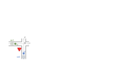
Figure 7: The program ADS (automated driving system, Program 12). car2 should yield and it notices car1 at time a. We sample settings (the initial position and velocity of car2) under which a near miss happens with car2 travelling with $\geq$ 30 km/h.

Table 1: experimental results. Experiments ran for designated timeout seconds, or until 500K samples were obtained (“$\geq$500K”). For some programs, the ground truth is known, and the KL-divergence from it is shown. When the ground truth is unknown, the mean and standard deviation is shown. The numbers are the average of ten runs. Anglican-IPMCMC is not shown since for many programs it returned obviously wrong samples. See B for more details.

method (timeout) Schism (10 sec.) Schism (60 sec.) Schism (600 sec.) Anglican-RMH (60 sec.) Anglican-SMC (60 sec.) $\downarrow$ target program samples KL-div. samples KL-div. samples KL-div. samples KL-div. samples KL-div. unifCd(10) 3.07K 0.281 9.37K 0.0793 37.6K 0.0174 $\geq$500K 0.869 492K 0.0938 unifCd(20) 1.99K 0.416 6.82K 0.103 34.5K 0.02 376K 6.44 550 5.21 poisCd(6,20) 2.11K 0.0618 7.43K 0.00764 72.6K 0.000879 323K 0.000141 1.25K 0.108 poisCd(6,30) 1.14K 0.0726 8.84K 0.00577 98.4K 0.000294 0 — 0 — geomIt(0.5,20) 1.42K 0.261 4.97K 0.0425 20K 0.0114 139K 0.00119 0 — geomIt(0.1,5) 3.05K 2.08 8.54K 2.0 27.6K 1.98 411K 1.95 2.66K 1.95 geomIt(0.1,20) 1.31K 2.14 4.73K 2.04 20.1K 1.98 0 — 0 — mixed(0) 35.5K 0.0813 198K 0.0734 $\geq$500K 0.0724 457K 0.0738 $\geq$500K 0.0724 coin(0.1) 55.5K 1.67e-06 270K 6.82e-08 $\geq$500K 2.03e-08 $\geq$500K 4.65e-05 $\geq$500K 7.66e-06 coin(0.001) 55.4K 1.66e-06 270K 6.86e-08 $\geq$500K 2.05e-08 $\geq$500K 0.00204 280K 0.000143 samples mean $\pm$ std samples mean $\pm$ std samples mean $\pm$ std samples mean $\pm$ std samples mean $\pm$ std unifCd2(10) 2.34K 10.6 $\pm$ 3.35 7.07K 10.8 $\pm$ 3.45 26.8K 10.9 $\pm$ 3.51 214K 11.2 $\pm$ 3.67 266K 11.0 $\pm$ 3.59 unifCd2(20) 1.29K 20.3 $\pm$ 4.56 4.92K 20.7 $\pm$ 4.65 23.1K 20.9 $\pm$ 4.71 83K 21.6 $\pm$ 4.69 300 21.8 $\pm$ 2.26 geomIt2(0.5,20) 830 22.5 $\pm$ 0.258 3.32K 23.5 $\pm$ 1.02 14.7K 23.9 $\pm$ 1.33 38.8K 24.0 $\pm$ 1.44 0 — geomIt2(0.1,5) 2.24K 6.4 $\pm$ 0.535 6.27K 6.44 $\pm$ 0.575 21.3K 6.46 $\pm$ 0.594 134K 6.53 $\pm$ 0.636 0 — geomIt2(0.1,20) 860 22.2 $\pm$ 0.335 3.36K 22.5 $\pm$ 0.572 14.5K 22.5 $\pm$ 0.617 0 — 0 — obsLoop(3,10) 1.9K 10.0 $\pm$ 0.136 4.58K 10.0 $\pm$ 0.169 13.1K 10.1 $\pm$ 0.209 141K 10.1 $\pm$ 0.299 0 — obsLoop(3,12) 1.72K 12.0 $\pm$ 0.0772 4.27K 12.0 $\pm$ 0.153 12.4K 12.0 $\pm$ 0.172 0 — 0 — poisCdS(12) 100 15.0 $\pm$ 0.0 1.23K 20.3 $\pm$ 0.0209 7.28K 25.7 $\pm$ 1.25 16.5K 25.2 $\pm$ 1.38 9.3K 25.5 $\pm$ 1.31 poisCdS(3) 100 14.0 $\pm$ 0.0 1.21K 19.4 $\pm$ 0.168 13.5K 23.3 $\pm$ 1.06 0 — 0 — nestLp(1) 0 — 0 — 1.47K 9.41 $\pm$ 0.279 0 — 0 — nestLp(3) 0 — 0 — 1.22K 9.28 $\pm$ 0.238 0 — 0 — ADS(0.5) 0 — 0 — 14.3K 20.9 $\pm$ 1.13 0 — 0 —

Table 2: ablation studies. full blkl. blacklists both complete and incomplete flows; leaf blkl. only looks at complete flows. cond. prop. only does not blacklist; no cond. prop. does not even apply condition propagation. Timeout is set to 600 sec.

method Schism, full blkl. Schism, leaf blkl. Schism, cond. prop. only Schism, no cond. prop. Anglican-SMC $\downarrow$ target program samples KL-div. samples KL-div. samples KL-div. samples KL-div. unifCd(10) 37.6K 0.0174 29.6K 0.0244 23.4K 0.0295 13.1K 2.18 $\geq$500K 0.0944 unifCd(20) 34.5K 0.02 22.5K 0.0317 15.1K 0.0443 0 — 5.88K 2.9 poisCd(6,30) 98.4K 0.000294 15.6K 0.00312 11.3K 0.00647 0 — 0 — samples mean $\pm$ std samples mean $\pm$ std samples mean $\pm$ std samples mean $\pm$ std samples mean $\pm$ std nestLp(1) 1.47K 9.41 $\pm$ 0.279 0 — 0 — 0 — 0 — nestLp(3) 1.22K 9.28 $\pm$ 0.238 0 — 0 — 0 — 0 — ADS(0.5) 14.3K 20.9 $\pm$ 1.13 0 — 0 — 0 — 0 —

The programs mixed and coin have simple control structures (a couple of if branchings). For such programs, our control-data separation tends to have more overhead than advantage—compare the number of samples after 60 sec.

The other programs feature a while loop. With them we observe benefits of our combination of control-data separation and logical condition propagation. This is especially the case with harder instances, i.e. those with more restrictive conditioning (instances are sorted from easy to hard in Table 2). Schism can return samples of reasonable quality while Anglican struggles: see the results with poisCd and geomIt. See also unifCd, where KL-divergence differs a lot. Condition propagation is crucial here: by logical reasoning, Schism blacklists a number of shallow control flows, quickly digging into deeper flows. Those deeper flows have tiny likelihoods and thus hard to find for Anglican. At the same time, $\texttt{geomIt}(0.5,5),(0.5,20)$ show that Anglican can be much faster and more precise when conditioning is not harsh, even in presence of a while loop.

For many instances of the programs with while loops, IPMCMC ran very quickly but returned obviously wrong samples; see B. This seems to be because of the general challenge with MCMC walks traversing different control flows [DBLP:journals/corr/abs-1809-10756, Section 4.2].

The programs poisCdS and nestLp feature soft conditioning (by observe(normal(x,1)(o))), which Schism handles without problems. The programs nestLp and ADS have more complicated control structures—nested loops in nestLp and successive loops in ADS. For them, discovering feasible control flows is harder, resulting in $0$ samples for Schism after 60 sec. After 600 sec., however, Schism succeeds to obtain samples.

In Table 2, we compare the performance of Schism under different policies (full blkl. is default). We see that condition propagation and blacklisting both contribute significantly to sampling performance. In particular, for programs with complicated control structures such as nestLp and ADS, logical blacklisting of incomplete flows is crucial.

Overall, we observe that Schism’s combination of control-data separation and condition propagation successfully addresses the general challenge of compatibility between sampling and control structures. Its performance is especially superior in programs with 1) while loops and 2) restrictive conditioning (“rare events”). Programs with these features are widespread in many application domains.

One such application domain of great practical relevance is testing of automotive systems; see [DBLP:conf/cav/DreossiFGKRVS19] for a software science perspective of the domain. In that domain, indeed, many models involve while loops for describing vehicle dynamics, and hazards such as near misses are often rare events—a combination that Schism is suited to. The last point is demonstrated by our example ADS (Program 12, Figure 7). Application of the current framework to a wider variety of practical problems in the domain—including scenario sampling that involves sampling from discrete sets of options [QueirozBC19]—will require further scrutiny of the framework and its extension. This is an important direction of future work.

Appendix A Omitted Details

A.1 Derivation of Our Sampling Algorithm

Let $\Gamma$ be a pCFG; our goal is to draw samples from the distribution $\llbracket\Gamma\rrbracket^{\mathsf{st}}$ in (6). The relevant random variables are as follows: $N$ (the length of a complete control flow $\vec{l}$); $l_{1},\dotsc,l_{N}$ (the locations in the complete control flow $\raisebox{0.0pt}[0.0pt][0.0pt]{$\vec{l}$}=l_{1}\dotsc l_{N}$); and $\sigma_{1},\dotsc,\sigma_{N}$ (the memory states at those locations).

By marginalization and the definition of conditional probability, we can transform our target distribution $p(\llbracket e_{\mathrm{final}}\rrbracket_{\sigma_{N}}\in\mathrm{d}v\mid\Gamma)$ as follows.

$$p(\llbracket e_{\mathrm{final}}\rrbracket_{\sigma_{N}}\in\mathrm{d}v\mid\Gamma)$$

$$=\textstyle\int_{\sigma_{N}}\,\delta_{\llbracket e_{\mathrm{final}}\rrbracket_{\sigma_{N}}}(\mathrm{d}v)\cdot p(\mathrm{d}\sigma_{N}\mid\Gamma)$$

$$=\textstyle\int_{\sigma_{1:N},l_{1:N}}\,\delta_{\llbracket e_{\mathrm{final}}\rrbracket_{\sigma_{N}}}(\mathrm{d}v)\cdot p(\mathrm{d}\sigma_{1:N}\times\mathrm{d}l_{1:N}\mid\Gamma)\qquad\text{marginalization}$$

$$=\textstyle\int_{\sigma_{1:N},l_{1:N}}\,\delta_{\llbracket e_{\mathrm{final}}\rrbracket_{\sigma_{N}}}(\mathrm{d}v)\cdot p(\mathrm{d}\sigma_{1:N}\mid l_{1:N},\Gamma)\cdot p(\mathrm{d}l_{1:N}\mid\Gamma)\qquad\text{conditional probabilities}$$

$$=\textstyle\int_{l_{1:N}}\bigl{(}\,\textstyle\int_{\sigma_{1:N}}\,\delta_{\llbracket e_{\mathrm{final}}\rrbracket_{\sigma_{N}}}(\mathrm{d}v)\cdot p(\mathrm{d}\sigma_{1:N}\mid l_{1:N},\Gamma)\,\bigr{)}\cdot p(\mathrm{d}l_{1:N}\mid\Gamma)$$

$$=\textstyle\int_{l_{1:N}}\bigl{(}\,\textstyle\int_{\sigma_{1:N}}\,p(\llbracket e_{\mathrm{final}}\rrbracket_{\sigma_{N}}\in\mathrm{d}v\mid\sigma_{N})\cdot p(\mathrm{d}\sigma_{1:N}\mid l_{1:N},\Gamma)\,\bigr{)}\cdot p(\mathrm{d}l_{1:N}\mid\Gamma)$$

The last expression justifies the following hierarchical sampling scheme. At the top level, we sample a control flow $l_{1:N}$ from the distribution $p(\mathrm{d}l_{1:N}\mid\Gamma)$; at the bottom level, for each control flow sample $l_{1:N}$, we sample data sequences $\sigma_{1:N}$, in the way that is conditioned by the fixed control flow $l_{1:N}$. The latter corresponds to sampling data from the straight-line program $\mathrm{SLP}(l_{1:N})$.

A.2 Multi-Armed Sampling

In our hierarchical sampling framework in Figure 1, we formulate the top-level control flow sampling as the infinite-armed sampling problem. As a step towards this problem, here we introduce and study the multi-armed sampling problem; the infinite-armed sampling problem is its variation with infinitely many arms.

A.2.1 The Multi-Armed Sampling Problem

The setting is informally described as follows. We have arms $\{1,2,\dotsc,K\}$, and each arm $k$ comes with its likelihood $p_{k}$. Our goal is to sample (or “pull”) arms from the set $\{1,2,\dotsc,K\}$ according to the likelihoods $p_{1},\dotsc,p_{K}$.

The challenge, however, is that the likelihoods $p_{1},\dotsc,p_{K}$ are not know a priori. We assume that, if we pull an arm $k$ at time $t$, we sample a random variable which is denoted by $X_{k,t}$. We further assume that $X_{k,t}$ is a random variable such that

• its mean is the (unknown) true likelihood $p_{k}$ of the arm $k$, and

• it is time-homogeneous, i.e.  $X_{k,1},X_{k,2},\dotsc$ are i.i.d.

Note that the problem is a “sampling-variant” of the classic multi-armed bandit (MAB) problem in reinforcement learning (RL). In MAB, the goal is to optimize—specifically, to maximize cumulative likelihood values—instead of to sample. MAB is an exemplar of the exploration-exploitation trade-off in RL: by engaging the greedy (or “exploitation-only”) strategy of keep pulling the empirically best-performing arm, one runs the risk of missing the actual best-performing arm, in case the latter happens to have performed empirically worse.

We formally state the problem. For the ease of theoretical analysis, we assume that the true likelihoods $p_{k}$, as well as the observed ones $X_{k,t}$, all take their values in the unit interval $[0,1]$.

Definition 20 (the (finite) multi-armed sampling problem).

• Given: a finite set $\mathcal{K}=\{1,\dotsc,K\}$ of arms. Each arm $k\in\mathcal{K}$, when pulled, returns an observed likelihood that is given by a random variable $X_{k,t}$. We assume that $\{X_{k,t}\}_{t\in{\mathbb{Z}_{>0}}}$ is i.i.d., and that the mean of $X_{k,t}$ is $p_{k}$.

• Goal: pull one arm at each time $t\in{\mathbb{Z}_{>0}}$, producing a sequence of arms $k^{(1)},k^{(2)},\dotsc$ (where $k^{(t)}\in\mathcal{K}$ for each $t\in{\mathbb{Z}_{>0}}$), so that the vector

  $$\left(\,\textstyle\frac{T_{1}(T)}{T},\,\dotsc,\,\frac{T_{K}(T)}{T}\,\right),\quad\text{where $T_{k}(T)=\bigl{|}\{t\in[1,T]\mid k^{(t)}=k\}\bigr{|}$ is the \emph{visit count}, }$$ (16)

  converges to the vector $\left(\,\frac{p_{1}}{\sum_{k}p_{k}},\,\dotsc,\,\frac{p_{K}}{\sum_{k}p_{k}}\,\right)$ as $T\to\infty$. Here, the two vectors of length $K$ are understood as categorical distributions over the set $\{1,2,\dotsc,K\}$ of arms. Convergence here precisely means the one in Theorem 21.

A.2.2 An $\varepsilon$-Greedy Algorithm

Algorithm 4 An $\varepsilon$-greedy algorithm for (finite) multi-armed sampling

1:The setting of Definition 20 (with arms $1,\dotsc,K$), $T\in{\mathbb{Z}_{>0}}$, and $\varepsilon_{t}=(\frac{K\log t}{t})^{\frac{1}{3}}$ for each $t\in{\mathbb{Z}_{>0}}$

2:a sequence $k^{(1)},k^{(2)},\dotsc,k^{(T)}$ of arms from $\mathcal{K}=\{1,\dotsc,K\}$

3:$t\leftarrow 0$ $\triangleright$ Initialization

4:while $t<T$ do

5:     $t\leftarrow t+1$

6:     $\mathsf{explore?}\leftarrow\text{(sample from $[\mathsf{true}\mapsto\varepsilon_{t},\mathsf{false}\mapsto 1-\varepsilon_{t}]$)}$

7:     if $\mathsf{explore?}=\mathsf{true}$ then

8:         $k^{(t)}\leftarrow\text{(sampled from the uniform distribution over $\mathcal{K}$)}$

9:     else

10:         $k^{(t)}\leftarrow\text{(sampled according to the empirical likelihoods $\bigl{[}\hat{p}_{1,t-1},\dotsc,\hat{p}_{K,t-1}\bigr{]}$)}$      

11:     $p^{(t)}\leftarrow\text{(sampled from $X_{k,t}$)}$

We propose the algorithm shown in Algorithm 4, where $T_{k}(t)$ is the visit count from (16), and $\hat{p}_{k,t}$ is the empirical mean of likelihoods observed by pulling the arm $k$, that is,

$$\hat{p}_{k,t}=\frac{1}{T_{k}(t)}\sum_{s\in[1,t]\text{ such that }k^{(s)}=k}p^{(s)}\enspace.$$ (17)

The algorithm is exactly the same as the $\varepsilon$-greedy algorithm for MAB (for optimization), except that in Line 10, we sample according to the empirical likelihoods instead of pulling the empirically best-performing arm. The “exploration” rate $\varepsilon_{t}=(\frac{K\log t}{t})^{\frac{1}{3}}$ is the same as the one commonly used for MAB, too; see e.g. [Slivkins19, BubeckC12].

A.2.3 Convergence of the $\varepsilon$-Greedy Algorithm

It turns out that our $\varepsilon$-Greedy algorithm (Algorithm 4) indeed achieves the goal described in Definition 20, as we show in Theorem 21. The convergence speed is slower, however, compared to the MAB (optimization) case. For MAB, the $\varepsilon$-Greedy algorithm achieves a regret bound $T^{2/3}\cdot O(K\log T)^{1/3}$, that is, regret $O(K\log T/T)^{1/3}$ per trial. See [Slivkins19].

Theorem 21.

The output $k^{(1)},k^{(2)},\dotsc,k^{(T)}$ of Algorithm 4 achieves the goal of Definition 20. Specifically, we have

$$\left|\,\frac{\mathbb{E}(T_{k}(T))}{T}-\frac{p_{k}}{\sum_{k}p_{k}}\,\right|=O\Bigl{(}K^{\frac{7}{3}}\Bigl{(}\frac{\log T}{T}\Bigr{)}^{\frac{1}{4}}\Bigr{)}\quad\text{for each $k\in\mathcal{K}$.}$$ (18)

Proof.

We follow the proof structure outlined in [Slivkins19]—it emphasizes the role of so-called clean events—adapting it to the current sampling setting.

In what follows, we proceed leaving two constants $\alpha,\beta$ as parameters—$\alpha$ will appear in (25), and $\beta$ occurs in the definition of the exploration rate

$$\varepsilon_{t}=\left(\frac{K\log t}{t}\right)^{\beta}\enspace.$$

We assume $0<\alpha,\beta<1$. In the course of the proof, we collect constraints on $\alpha$ and $\beta$, and in the end we choose the values of $\alpha,\beta$ so that the resulting error bound is optimal. We will see that $\alpha=\frac{1}{4}$ and $\beta=\frac{1}{3}$ are optimal, yielding the exploration rate $\varepsilon_{t}$ in Algorithm 4.

Let us consider the following events.

$$E_{1}(t)\quad\text{(where $t\in[1,T]$)}:$$ (19)

$$\quad\left[\parbox[c]{303.53267pt}{ \begin{math}\forall k\in\mathcal{K}.\,\forall s\in[1,t].\quad\bigl{|}\,\hat{p}_{k,s}-p_{k}\,\bigr{|}\leq\sqrt{\frac{\log T}{T_{k}(s)}},\end{math} \quad and \\ \begin{math}\forall k\in\mathcal{K}.\quad T_{k}(t)\geq\frac{t^{1-\beta}\bigl{(}\log t\bigr{)}^{\beta}}{K^{1-\beta}}-\sqrt{t\bigl{(}\log t-\log(\log t)\bigr{)}}\end{math} }\right]$$

We claim that

$$\mathbb{P}(E_{1}(t))=1-O\Bigl{(}K\Bigl{(}\frac{\log t}{t}\Bigr{)}^{2}\Bigr{)}\enspace.$$ (20)

To see this, first observe that

$$\mathbb{P}\left(\bigl{|}\,\hat{p}_{k,s}-p_{k}\,\bigr{|}\leq\sqrt{\frac{\log T}{T_{k}(s)}}\right)\geq 1-\frac{2}{T^{2}}$$ (21)

holds by Hoeffding’s inequality for each $k$ and $s$. For the second condition in $E_{1}(t)$ in (19), we argue as follows. According to Algorithm 4, the visit count $T_{k}(t)$ is the sum of the number of the exploration picks (Line 8) and that of the usual picks (Line 10). By counting only the exploration picks, and also noting that $\varepsilon_{t}=(\frac{K\log t}{t})^{\beta}$ is decreasing with respect to $t$, we observe that

$$T_{k}(t)\geq\mathsf{RB}(\varepsilon_{t}K^{-1},t)=\mathsf{RB}\left(\frac{(\log t)^{\beta}}{K^{1-\beta}t^{\beta}},\,t\right),$$ (22)

where $\mathsf{RB}(\alpha,s)$ is the “repeated Bernoulli” random variable for the number of heads when a coin with bias $\alpha$ is tossed $s$ times. This observation is used in the following reasoning.

$$\mathbb{P}\left[T_{k}(t)\geq\frac{t^{1-\beta}(\log t)^{\beta}}{K^{1-\beta}}-\sqrt{t\bigl{(}\log t-\log(\log t)\bigr{)}}\right]$$ (23)

$$\geq\mathbb{P}\left[\mathsf{RB}\left(\frac{(\log t)^{\beta}}{K^{1-\beta}t^{\beta}},\,t\right)\geq\frac{t^{1-\beta}(\log t)^{\beta}}{K^{1-\beta}}-\sqrt{t\bigl{(}\log t-\log(\log t)\bigr{)}}\right]$$

$$\geq 1-\exp\left(-2\left(\sqrt{\frac{\log t-\log(\log t)}{t}}\right)^{2}t\right)\qquad\text{by Hoeffding's inequality}$$

$$=1-\left(\frac{\log t}{t}\right)^{2}\enspace.$$

Combining (21) and (23) we obtain

$$\mathbb{P}(E_{1}(t))\geq 1-KT\frac{2}{T^{2}}-K\left(\frac{\log t}{t}\right)^{2}$$ (24)

which proves the claim (20). Note that, in deriving (24), we used the following basic principle:

$$\mathbb{P}(\bigwedge_{i=1}^{n}A_{i})\;=\;1-\mathbb{P}(\bigvee_{i=1}^{n}\overline{A_{i}})\;\geq\;1-\sum_{i=1}^{n}\mathbb{P}(A_{i})\enspace.$$

Towards the statement (18) of the proposition, we introduce a constant

$$L=\lceil T^{1-\alpha}(\log T)^{\alpha}\rceil\enspace,$$ (25)

where $\alpha$ is a parameter that will later be chosen by optimization (as we discussed at the beginning of the proof). The intuition of $L$ is as follows: the first $L$ samples $k^{(1)},\dotsc,k^{(L)}$ (out of $T$ samples in total) are transient ones, and they are inessential in the convergence guarantee in Theorem 21.

We focus on suitable clean events (namely $E_{1}(L)\land E_{1}(T)$), and estimate the deviation from the true likelihood $\frac{p_{k}}{\sum_{k\in\mathcal{K}}p_{k}}$.

$$\mathbb{E}\left(\frac{T_{k}(T)}{T}-\frac{p_{k}}{\sum_{k\in\mathcal{K}}p_{k}}\;\bigg{|}\;E_{1}(L)\land E_{1}(T)\right)$$

$$=\mathbb{E}\left(\frac{T_{k}(L)}{T}+\frac{1}{T}\sum_{t=L+1}^{T}\frac{\varepsilon_{t}}{K}+\frac{1}{T}\sum_{t=L+1}^{T}(1-\varepsilon_{t})\frac{\hat{p}_{k,t}}{\sum_{k\in\mathcal{K}}\hat{p}_{k,t}}-\frac{p_{k}}{\sum_{k\in\mathcal{K}}p_{k}}\;\bigg{|}\;E_{1}(L)\land E_{1}(T)\right)$$

$$\leq\mathbb{E}\left(\frac{L}{T}+\frac{\varepsilon_{L}(T-L)}{KT}+\frac{1}{T}\sum_{t=L+1}^{T}\frac{p_{k}+\sqrt{\frac{\log T}{T_{k}(t)}}}{\sum_{k\in\mathcal{K}}\left(p_{k}-\sqrt{\frac{\log T}{T_{k}(t)}}\right)}-\frac{p_{k}}{\sum_{k\in\mathcal{K}}p_{k}}\;\Bigg{|}\;E_{1}(L)\land E_{1}(T)\right)$$

by $$T_{k}(L)\leq L \varepsilon_{t}\leq\varepsilon_{L} t\in[L+1,T] E_{1}(T)$$, for , and

$$\leq\mathbb{E}\left(\frac{L}{T}+\frac{\varepsilon_{L}T}{KT}+\frac{1}{T}\sum_{t=L+1}^{T}\frac{p_{k}+\sqrt{\frac{\log T}{T_{k}(L)}}}{\sum_{k\in\mathcal{K}}\left(p_{k}-\sqrt{\frac{\log T}{T_{k}(L)}}\right)}-\frac{p_{k}}{\sum_{k\in\mathcal{K}}p_{k}}\;\Bigg{|}\;E_{1}(L)\land E_{1}(T)\right)$$

by $$T_{k}(L)\leq T_{k}(t) t\in[L+1,T]$$ for

$$\leq\mathbb{E}\left(\frac{L}{T}+\frac{\varepsilon_{L}}{K}+\left(\frac{p_{k}+\sqrt{\frac{\log T}{T_{k}(L)}}}{\sum_{k\in\mathcal{K}}\left(p_{k}-\sqrt{\frac{\log T}{T_{k}(L)}}\right)}-\frac{p_{k}}{\sum_{k\in\mathcal{K}}p_{k}}\right)\;\Bigg{|}\;E_{1}(L)\land E_{1}(T)\right)$$ (26)

We shall bound, from above, the three terms in the last expression.

$$\frac{L}{T} =O\left(\left(\frac{\log T}{T}\right)^{\alpha}\right)$$ (27)

$$\frac{\varepsilon_{L}}{K} =\frac{1}{K}\left(\frac{K\log L}{L}\right)^{\beta}$$

$$=O\left(\frac{1}{K^{1-\beta}}\frac{\bigl{(}(1-\alpha)\log T+\alpha\log(\log T)\bigr{)}^{\beta}}{T^{\beta(1-\alpha)}(\log T)^{\alpha\beta}}\right)$$

$$=O\left(\frac{1}{K^{1-\beta}}\left(\frac{\log T}{T}\right)^{\beta(1-\alpha)}\right)$$ (28)

On the third term in (26), we proceed as follows.

$$T_{k}(L) \geq\frac{L^{1-\beta}\bigl{(}\log L\bigr{)}^{\beta}}{K^{1-\beta}}-\sqrt{L\bigl{(}\log L-\log(\log L)\bigr{)}}\quad\text{by $E_{1}(L)$,}$$

$$\frac{L^{1-\beta}(\log L)^{\beta}}{K^{1-\beta}} =\Theta\Bigl{(}T^{(1-\alpha)(1-\beta)}(\log T)^{\alpha(1-\beta)}\bigl{(}\log(T^{1-\alpha}(\log T)^{\alpha})\bigr{)}^{\beta}\frac{1}{K^{1-\beta}}\Bigr{)}$$

$$=\Theta\Bigl{(}T^{(1-\alpha)(1-\beta)}(\log T)^{\alpha(1-\beta)}\bigl{(}(1-\alpha)\log T+\alpha\log(\log T)\bigr{)}^{\beta}\frac{1}{K^{1-\beta}}\Bigr{)}$$

$$=\Theta\bigl{(}T^{(1-\alpha)(1-\beta)}(\log T)^{\alpha(1-\beta)+\beta}\frac{1}{K^{1-\beta}}\bigr{)}$$

$$=\Theta\bigl{(}T^{(1-\alpha)(1-\beta)}(\log T)^{1-(1-\alpha)(1-\beta)}\frac{1}{K^{1-\beta}}\bigr{)}$$

by $$\alpha(1-\beta)+\beta=1-(1-\alpha)(1-\beta)$$, (29)

$$\sqrt{L\bigl{(}\log L-\log(\log L)\bigr{)}}$$

$$=\Theta\left(\left(T^{1-\alpha}(\log T)^{\alpha}\bigl{(}(1-\alpha)\log T+\alpha\log(\log T)-\log((1-\alpha)\log T+\alpha\log(\log T))\bigr{)}\right)^{\frac{1}{2}}\right)$$

$$=\Theta\left(T^{\frac{1-\alpha}{2}}(\log T)^{\frac{1+\alpha}{2}}\right)\enspace.$$ (30)

Let us now impose a condition

$$(1-\alpha)(1-\beta)>\frac{1-\alpha}{2}\enspace,$$ (31)

which will be taken into account when we choose the values of $\alpha,\beta$ in the end. This assumption implies that (29) dominates (30), and hence that

$$T_{k}(L)\;\geq\;\Theta\left(T^{(1-\alpha)(1-\beta)}(\log T)^{1-(1-\alpha)(1-\beta)}\frac{1}{K^{1-\beta}}\right)\enspace.$$ (32)

We continue the estimation of the third term in (26). Let $\delta$ denote $\sqrt{\frac{\log T}{T_{k}(L)}}$ occurring therein. It follows from (32) that $\delta\leq\Theta\Bigl{(}K^{\frac{1-\beta}{2}}\left(\frac{\log T}{T}\right)^{\frac{(1-\alpha)(1-\beta)}{2}}\Bigr{)}$; in particular, $\delta$ tends to $0$ as $T\to\infty$ since $\alpha,\beta\in(0,1)$.

$$\left(\frac{p_{k}+\delta}{\sum_{k\in\mathcal{K}}\left(p_{k}-\delta\right)}-\frac{p_{k}}{\sum_{k\in\mathcal{K}}p_{k}}\right) =\left(\frac{p_{k}+\delta}{(\sum_{k\in\mathcal{K}}p_{k})-K\delta}-\frac{p_{k}}{\sum_{k\in\mathcal{K}}p_{k}}\right)$$

$$=O\left((p_{k}+\delta)\left(\frac{1}{\sum_{k\in\mathcal{K}}p_{k}}+\frac{2K\delta}{\left(\sum_{k\in\mathcal{K}}p_{k}\right)^{2}}\right)-\frac{p_{k}}{\sum_{k\in\mathcal{K}}p_{k}}\right)$$ (33)

$$=O\left(\frac{\delta}{\sum_{k\in\mathcal{K}}p_{k}}+\frac{2K\delta(p_{k}+\delta)}{\left(\sum_{k\in\mathcal{K}}p_{k}\right)^{2}}\right)\qquad$$

$$=O\left(K\delta\right)$$

$$=O\Bigl{(}K^{\frac{3-\beta}{2}}\left(\frac{\log T}{T}\right)^{\frac{(1-\alpha)(1-\beta)}{2}}\Bigr{)}\enspace.$$ (34)

In (33) we used the following general fact. Let $a$ a constant, and $\varphi$ be a function of $T$ that takes nonnegative values and tends to $0$ as $T\to\infty$. Then $\frac{1}{a-\varphi}=O(\frac{1}{a}+\frac{2\varphi}{a^{2}})$.

Combining (26) and (27,28,34), we obtain, for each $k\in\mathcal{K}=\{1,2,\dotsc,K\}$,

$$\mathbb{E}\left(\frac{T_{k}(T)}{T}-\frac{p_{k}}{\sum_{k\in\mathcal{K}}p_{k}}\;\bigg{|}\;E_{1}(L)\land E_{1}(T)\right)$$

$$=O\left(\left(\frac{\log T}{T}\right)^{\alpha}+\frac{1}{K^{1-\beta}}\left(\frac{\log T}{T}\right)^{\beta(1-\alpha)}+K^{\frac{3-\beta}{2}}\left(\frac{\log T}{T}\right)^{\frac{(1-\alpha)(1-\beta)}{2}}\right)\enspace.$$

Since $\sum_{k\in\mathcal{K}}\frac{T_{k}(T)}{T}=\sum_{k\in\mathcal{K}}\frac{p_{k}}{\sum_{k\in\mathcal{K}}p_{k}}=1$, we also obtain a lower bound of the difference, namely

$$\mathbb{E}\left(\frac{p_{k}}{\sum_{k\in\mathcal{K}}p_{k}}-\frac{T_{k}(T)}{T}\;\bigg{|}\;E_{1}(L)\land E_{1}(T)\right)$$

$$=\sum_{k^{\prime}\in\mathcal{K}\setminus\{k\}}\mathbb{E}\left(\frac{T_{k^{\prime}}(T)}{T}-\frac{p_{k^{\prime}}}{\sum_{k\in\mathcal{K}}p_{k}}\;\bigg{|}\;E_{1}(L)\land E_{1}(T)\right)$$

$$=O\left(K\left(\frac{\log T}{T}\right)^{\alpha}+K^{\beta}\left(\frac{\log T}{T}\right)^{\beta(1-\alpha)}+K^{\frac{5-\beta}{2}}\left(\frac{\log T}{T}\right)^{\frac{(1-\alpha)(1-\beta)}{2}}\right)\enspace.$$

Combining the above two, we obtain

$$\mathbb{E}\left(\;\bigg{|}\frac{T_{k}(T)}{T}-\frac{p_{k}}{\sum_{k\in\mathcal{K}}p_{k}}\bigg{|}\;\bigg{|}\;E_{1}(L)\land E_{1}(T)\right)$$ (35)

$$=O\left(K\left(\frac{\log T}{T}\right)^{\alpha}+K^{\beta}\left(\frac{\log T}{T}\right)^{\beta(1-\alpha)}+K^{\frac{5-\beta}{2}}\left(\frac{\log T}{T}\right)^{\frac{(1-\alpha)(1-\beta)}{2}}\right)\enspace.$$

We are ready to show the statement of the proposition.

$$\left|\frac{\mathbb{E}(T_{k}(T))}{T}-\frac{p_{k}}{\sum_{k}p_{k}}\right|$$

$$=\mathbb{E}\left(\left|\,\frac{T_{k}(T)}{T}-\frac{p_{k}}{\sum_{k}p_{k}}\,\right|\,\Bigg{|}\,E_{1}(L)\land E_{1}(T)\right)\cdot\mathbb{P}\bigl{(}\,E_{1}(L)\land E_{1}(T)\,\bigr{)}$$

$$\quad+\mathbb{E}\left(\left|\,\frac{T_{k}(T)}{T}-\frac{p_{k}}{\sum_{k}p_{k}}\,\right|\,\Bigg{|}\,\overline{E_{1}(L)}\lor\overline{E_{1}(T)}\right)\cdot\mathbb{P}\bigl{(}\,\overline{E_{1}(L)}\lor\overline{E_{1}(T)}\,\bigr{)}$$

$$\leq\mathbb{E}\left(\left|\,\frac{T_{k}(T)}{T}-\frac{p_{k}}{\sum_{k}p_{k}}\,\right|\,\Bigg{|}\,E_{1}(L)\land E_{1}(T)\right)+\mathbb{P}\bigl{(}\,\overline{E_{1}(L)}\lor\overline{E_{1}(T)}\,\bigr{)}$$

$$=O\left(K\left(\frac{\log T}{T}\right)^{\alpha}+K^{\beta}\left(\frac{\log T}{T}\right)^{\beta(1-\alpha)}+K^{\frac{5-\beta}{2}}\left(\frac{\log T}{T}\right)^{\frac{(1-\alpha)(1-\beta)}{2}}\right)$$

$$\qquad\qquad+O\left(K\Bigl{(}\frac{\log L}{L}\Bigr{)}^{2}+K\Bigl{(}\frac{\log T}{T}\Bigr{)}^{2}\right)\qquad\text{by~{}(\ref{eq:E1Claiim},\ref{eq:boundForAbsValue}) }$$

$$=O\left(K\left(\frac{\log T}{T}\right)^{\alpha}+K^{\beta}\left(\frac{\log T}{T}\right)^{\beta(1-\alpha)}+K^{\frac{5-\beta}{2}}\left(\frac{\log T}{T}\right)^{\frac{(1-\alpha)(1-\beta)}{2}}\right.$$

$$\qquad\qquad\left.+K\left(\frac{\log T}{T}\right)^{2(1-\alpha)}+K\Bigl{(}\frac{\log T}{T}\Bigr{)}^{2}\right)$$ (36)

We now choose the parameters $\alpha,\beta\in(0,1)$ so that (36) is optimal, that is, so that the minimum of the powers of the five terms (namely $\alpha$, $\beta(1-\alpha)$, $\frac{(1-\alpha)(1-\beta)}{2}$, $2(1-\alpha)$, $2$) is maximal. The choice turns out to be $\alpha=\frac{1}{4},\beta=\frac{1}{3}$, which yields $\alpha=\beta(1-\alpha)=\frac{(1-\alpha)(1-\beta)}{2}=1/4$, and $2(1-\alpha)=3/2$. The choice of $\alpha,\beta$ satisfies the additional condition (31) that we introduced in the course of the proof, too.

The bound (36) under the above choice of $\alpha,\beta$ yields the desired bound. This concludes the proof. ∎

A.3 Comparison with the Flow Sampling Strategy in [ZhouYTR20]

In [ZhouYTR20], traversing different “sub-programs” (that correspond to control flows in this paper) is thought of as a problem of resource allocation. Their solution to the problem is a UCB-based algorithm adapted from [RainforthZLTWYvdM18]. Their algorithm do not aim to sample flows in proportion to their likelihoods; instead, it allocates more resources to those flows whose flow likelihood samples have a larger variance. Doing so follows ideas in stratified sampling and accelerates convergence of the mean value of flow likelihoods samples. See [ZhouYTR20, Appendix F].

One can argue as follows: in probabilistic program inference, our interest is in return values, instead of in flow likelihoods. This suggests a modification of the algorithm in [ZhouYTR20], so that it samples more often those control flows that have a larger variance of return value samples.

Even in the last modification, the stratified sampling-style variance-guided resource allocation strategy aims at fast convergence of the mean value, instead of the return value distribution itself. This does not suit such cases in which our interest is beyond the mean value. For example, in automotive system safety, international standards such as ISO 26262 require rare hazards to be identified and addressed. See the example ADS in Program 12 & Figure 7.

With the arguments in the above in mind, proportional flow sampling emerges as a viable alternative. Not knowing 1) the data distributions for different control flows or 2) the user’s statistical interest (mean, variance, other statistics, or the return value distribution itself), choosing control flows in proportion to their likelihoods seems to be the best one can do. This justifies our study of IAS sampling of control flows; further comparison is future work.

A.4 Justification of Flow Likelihood Estimation

The equality (15) in Section 3.2 is shown as follows. Here we use the definition of conditional probability; we also use the principle of conditional independence (i.e. the Markovian property of pCFGs) to derive equalities such as $p(\sigma_{3}\mid\sigma_{1:2},l_{1:3},\Gamma)=p(\sigma_{3}\mid\sigma_{2},l_{2:3},\Gamma)$. We also note that the set of complete control flows $l_{1:N}$ is countable and thus it makes sense to speak of the probability $p(l_{1:N}\mid\Gamma)$.

$$\begin{array}[]{ll}p(l_{1:N}\mid\Gamma)&=\int_{\sigma_{1:N}}\,p(\mathrm{d}\sigma_{1:N},l_{1:N}\mid\Gamma)\\ &=\int_{\sigma_{1:N}}\,p(\mathrm{d}\sigma_{1},l_{1}\mid\Gamma)\,p(\mathrm{d}\sigma_{2:N},l_{2:N}\mid\sigma_{1},l_{1},\Gamma)\\ &=\int_{\sigma_{1:N}}\,p(\mathrm{d}\sigma_{1},l_{1}\mid\Gamma)\,p(l_{2}\mid\sigma_{1},l_{1},\Gamma)\,p(\mathrm{d}\sigma_{2}\mid\sigma_{1},l_{1:2},\Gamma)\,p(\mathrm{d}\sigma_{3:N},l_{3:N}\mid\sigma_{1:2},l_{1:2},\Gamma)\\ &=\cdots\\ &=\int_{\sigma_{1:N}}\,p(\mathrm{d}\sigma_{1},l_{1}\mid\Gamma)\cdot\left(\prod_{k=2}^{N}p(l_{k}\mid\sigma_{k-1},l_{k-1},\Gamma)\right)\cdot\left(\prod_{k=2}^{N}p(\mathrm{d}\sigma_{k}\mid\sigma_{k-1},l_{k-1:k},\Gamma)\right)\end{array}$$ (37)

Appendix B Supplementary Experimental Results

The following experiment data is supplementary to Section 4. The new target programs (with parameters) are in Program 13–14.

Prog.  13: coin(bias)

⬇

bool c1, c2 := true;

ifp (bias)

then c1 := true;

else c1 := false;

ifp (bias)

then c2 := true;

else c2 := false;

observe(!(c1 = c2));

return(c1);

Prog.  14: obsLoop(x0,n0)

⬇

double x := 0;

double y := 0;

int n := 0;

while (x < x0) {

n := n + 1;

y $\sim$ normal(1,1);

observe(0 <= y <= 2);

x := x + y;}

observe(n >= n0);

return(n);

Table 3: experimental results with more details, supplementing Table 2.

Comparing our proposal (Schism) with Anglican (with different sampling algorithms). “A.” stands for Anglican. Experiments ran for designated timeout seconds, or until 500K samples were obtained (marked with “$\geq$500K”). For the first group of programs, the ground truth is known, so the KL-divergence from it to the samples is shown. For the latter programs, the ground truth is not known, so the mean and standard deviation is shown. The numbers are the average of ten runs. method (timeout) Schism (10 sec.) Schism (60 sec.) Schism (600 sec.) A.-RMH (60 sec.) A.-SMC (60 sec.) A.-IPMCMC (60 sec.) A.-RMH (600 sec.) A.-SMC (600 sec.) A.-IPMCMC (600 sec.) target program samples KL-div. samples KL-div. samples KL-div. samples KL-div. samples KL-div. samples KL-div. samples KL-div. samples KL-div. samples KL-div. unifCd(10) 3.07K 0.281 9.37K 0.0793 37.6K 0.0174 $\geq$500K 0.869 492K 0.0938 0 — $\geq$500K 0.866 $\geq$500K 0.0944 0 — unifCd(15) 2.86K 0.34 7.92K 0.0983 35.7K 0.0185 $\geq$500K 3.96 18.1K 1.83 0 — $\geq$500K 3.73 179K 0.32 0 — unifCd(18) 2.18K 0.373 7.22K 0.104 35.5K 0.019 442K 6.03 2.15K 3.9 0 — $\geq$500K 5.76 21.1K 1.7 0 — unifCd(20) 1.99K 0.416 6.82K 0.103 34.5K 0.02 376K 6.44 550 5.21 0 — $\geq$500K 6.5 5.88K 2.9 0 — poisCd(6,20) 2.11K 0.0618 7.43K 0.00764 72.6K 0.000879 323K 0.000141 1.25K 0.108 $\geq$500K inf $\geq$500K 0.000108 14.9K 0.0223 $\geq$500K inf poisCd(6,30) 1.14K 0.0726 8.84K 0.00577 98.4K 0.000294 0 — 0 — $\geq$500K inf 0 — 0 — $\geq$500K inf poisCd(3,20) 1.93K 0.0308 15.1K 0.00178 152K 6.49e-05 0 — 0 — $\geq$500K inf 0 — 0 — $\geq$500K inf poisCd(3,30) 0 — 0 — 0 — 0 — 0 — $\geq$500K nan 0 — 0 — $\geq$500K nan geomIt(0.5,5) 3.11K 0.0881 8.34K 0.0201 27.7K 0.00646 324K 0.000158 $\geq$500K 0.000496 $\geq$500K 0.000726 $\geq$500K 0.0001 $\geq$500K 0.000551 $\geq$500K 0.000708 geomIt(0.5,20) 1.42K 0.261 4.97K 0.0425 20K 0.0114 139K 0.00119 0 — $\geq$500K inf $\geq$500K 0.0002 2.2K 0.162 $\geq$500K inf geomIt(0.1,5) 3.05K 2.08 8.54K 2.0 27.6K 1.98 411K 1.95 2.66K 1.95 $\geq$500K inf $\geq$500K 1.95 28.9K 1.97 $\geq$500K inf geomIt(0.1,20) 1.31K 2.14 4.73K 2.04 20.1K 1.98 0 — 0 — $\geq$500K inf 0 — 0 — $\geq$500K inf mixed(0) 35.5K 0.0813 198K 0.0734 $\geq$500K 0.0724 457K 0.0738 $\geq$500K 0.0724 $\geq$500K 0.0729 $\geq$500K 0.0729 $\geq$500K 0.0724 $\geq$500K 0.0733 coin(0.1) 55.5K 1.67e-06 270K 6.82e-08 $\geq$500K 2.03e-08 $\geq$500K 4.65e-05 $\geq$500K 7.66e-06 $\geq$500K 7.32e-06 $\geq$500K 1.38e-05 $\geq$500K 6.74e-06 $\geq$500K 3.9e-06 coin(0.001) 55.4K 1.66e-06 270K 6.86e-08 $\geq$500K 2.05e-08 $\geq$500K 0.00204 280K 0.000143 $\geq$500K 0.000332 $\geq$500K 0.00386 $\geq$500K 3.91e-05 $\geq$500K 0.000804 coin(0.00001) 0 — 0 — 0 — 0 — 0 — 0 — 0 — 0 — 0 — samples mean $\pm$ std samples mean $\pm$ std samples mean $\pm$ std samples mean $\pm$ std samples mean $\pm$ std samples mean $\pm$ std samples mean $\pm$ std samples mean $\pm$ std samples mean $\pm$ std unifCd2(10) 2.34K 10.6 $\pm$ 3.35 7.07K 10.8 $\pm$ 3.45 26.8K 10.9 $\pm$ 3.51 214K 11.2 $\pm$ 3.67 266K 11.0 $\pm$ 3.59 $\geq$500K 11.0 $\pm$ 3.69 $\geq$500K 10.9 $\pm$ 3.54 $\geq$500K 11.0 $\pm$ 3.63 $\geq$500K 10.9 $\pm$ 3.65 unifCd2(15) 1.73K 15.4 $\pm$ 4.0 5.77K 15.8 $\pm$ 4.11 24.8K 15.9 $\pm$ 4.17 168K 15.5 $\pm$ 3.96 8.67K 16.0 $\pm$ 4.25 $\geq$500K 11.9 $\pm$ 7.12 $\geq$500K 15.8 $\pm$ 4.09 95.2K 16.0 $\pm$ 4.28 $\geq$500K 12.5 $\pm$ 7.13 unifCd2(18) 1.53K 18.4 $\pm$ 4.33 5.06K 18.7 $\pm$ 4.44 23.8K 18.9 $\pm$ 4.52 89.8K 18.7 $\pm$ 4.35 1.37K 19.2 $\pm$ 4.86 $\geq$500K 4.0 $\pm$ 5.72 $\geq$500K 19.2 $\pm$ 4.4 12.2K 18.9 $\pm$ 4.73 $\geq$500K 4.47 $\pm$ 6.18 unifCd2(20) 1.29K 20.3 $\pm$ 4.56 4.92K 20.7 $\pm$ 4.65 23.1K 20.9 $\pm$ 4.71 83K 21.6 $\pm$ 4.69 300 21.8 $\pm$ 2.26 $\geq$500K 2.54 $\pm$ 3.49 463K 22.2 $\pm$ 4.72 3.5K 20.8 $\pm$ 4.83 $\geq$500K 2.35 $\pm$ 2.95 poisCd2(6,20) 1.45K 18.2 $\pm$ 0.429 4.82K 18.4 $\pm$ 0.673 35K 18.5 $\pm$ 0.752 98.4K 18.5 $\pm$ 0.801 4.28K 18.4 $\pm$ 0.713 $\geq$500K 13.7 $\pm$ 6.16 $\geq$500K 18.5 $\pm$ 0.806 44.3K 18.5 $\pm$ 0.781 $\geq$500K 13.9 $\pm$ 5.85 poisCd2(6,30) 1.03K 26.5 $\pm$ nan 3.98K 27.1 $\pm$ 0.512 41.7K 27.2 $\pm$ 0.64 0 — 0 — $\geq$500K 6.0 $\pm$ 2.45 0 — 0 — $\geq$500K 6.0 $\pm$ 2.45 poisCd2(3,20) 1.45K 18.1 $\pm$ 0.323 6.97K 18.2 $\pm$ 0.444 69.8K 18.2 $\pm$ 0.496 0 — 0 — $\geq$500K 3.0 $\pm$ 1.73 209K 18.2 $\pm$ 0.485 0 — $\geq$500K 3.0 $\pm$ 1.73 poisCd2(3,30) 1.45K 26.0 $\pm$ nan 10.9K 26.0 $\pm$ nan 112K 26.0 $\pm$ nan 0 — 0 — $\geq$500K 3.0 $\pm$ 1.73 0 — 0 — $\geq$500K 3.0 $\pm$ 1.73 geomIt2(0.5,5) 2.13K 7.35 $\pm$ 0.934 6.21K 7.63 $\pm$ 1.18 21K 7.79 $\pm$ 1.35 191K 7.96 $\pm$ 1.54 $\geq$500K 7.91 $\pm$ 1.53 $\geq$500K 7.91 $\pm$ 1.55 $\geq$500K 7.96 $\pm$ 1.55 $\geq$500K 7.91 $\pm$ 1.54 $\geq$500K 7.92 $\pm$ 1.55 geomIt2(0.5,20) 830 22.5 $\pm$ 0.258 3.32K 23.5 $\pm$ 1.02 14.7K 23.9 $\pm$ 1.33 38.8K 24.0 $\pm$ 1.44 0 — $\geq$500K 1.0 $\pm$ 1.42 400K 24.1 $\pm$ 1.55 0 — $\geq$500K 1.0 $\pm$ 1.42 geomIt2(0.1,5) 2.24K 6.4 $\pm$ 0.535 6.27K 6.44 $\pm$ 0.575 21.3K 6.46 $\pm$ 0.594 134K 6.53 $\pm$ 0.636 0 — $\geq$500K 0.111 $\pm$ 0.351 $\geq$500K 6.52 $\pm$ 0.634 0 — $\geq$500K 0.135 $\pm$ 0.449 geomIt2(0.1,20) 860 22.2 $\pm$ 0.335 3.36K 22.5 $\pm$ 0.572 14.5K 22.5 $\pm$ 0.617 0 — 0 — $\geq$500K 0.111 $\pm$ 0.352 0 — 0 — $\geq$500K 0.111 $\pm$ 0.351 obsLoop(3,5) 2.76K 5.13 $\pm$ 0.353 6.13K 5.17 $\pm$ 0.409 15K 5.2 $\pm$ 0.453 274K 5.22 $\pm$ 0.493 0 — 0 — $\geq$500K 5.22 $\pm$ 0.488 0 — 0 — obsLoop(3,8) 2.06K 8.05 $\pm$ 0.211 5.15K 8.09 $\pm$ 0.271 13.5K 8.1 $\pm$ 0.318 203K 8.11 $\pm$ 0.345 0 — 0 — $\geq$500K 8.11 $\pm$ 0.344 0 — 0 — obsLoop(3,10) 1.9K 10.0 $\pm$ 0.136 4.58K 10.0 $\pm$ 0.169 13.1K 10.1 $\pm$ 0.209 141K 10.1 $\pm$ 0.299 0 — 0 — $\geq$500K 10.1 $\pm$ 0.297 0 — 0 — obsLoop(3,12) 1.72K 12.0 $\pm$ 0.0772 4.27K 12.0 $\pm$ 0.153 12.4K 12.0 $\pm$ 0.172 0 — 0 — 0 — 0 — 0 — 0 — obsLoop(3,15) 1.09K 15.1 $\pm$ 0.0952 3.67K 15.1 $\pm$ 0.126 11.8K 15.0 $\pm$ 0.0757 0 — 0 — 0 — 0 — 0 — 0 — obsLoop(3,20) 262 20.0 $\pm$ 0.0 712 20.4 $\pm$ 0.0 3.92K 20.3 $\pm$ nan 0 — 0 — 0 — 0 — 0 — 0 — poisCdS(12) 100 15.0 $\pm$ 0.0 1.23K 20.3 $\pm$ 0.0209 7.28K 25.7 $\pm$ 1.25 16.5K 25.2 $\pm$ 1.38 9.3K 25.5 $\pm$ 1.31 111K 25.0 $\pm$ 1.86 296K 25.8 $\pm$ 1.42 96.4K 25.7 $\pm$ 1.41 $\geq$500K 25.5 $\pm$ 1.57 poisCdS(3) 100 14.0 $\pm$ 0.0 1.21K 19.4 $\pm$ 0.168 13.5K 23.3 $\pm$ 1.06 0 — 0 — 472K 7.93 $\pm$ 1.32 0 — 0 — $\geq$500K 7.94 $\pm$ 1.31 nestLp(0.1) 0 — 0 — 1.54K 9.5 $\pm$ 0.29 0 — 0 — 0 — 0 — 0 — 0 — nestLp(1) 0 — 0 — 1.47K 9.41 $\pm$ 0.279 0 — 0 — 0 — 0 — 0 — 0 — nestLp(3) 0 — 0 — 1.22K 9.28 $\pm$ 0.238 0 — 0 — 0 — 0 — 0 — 0 — ADS(0.5) 0 — 0 — 14.3K 20.9 $\pm$ 1.13 0 — 0 — $\geq$500K 11.1 $\pm$ 6.41 0 — 0 — $\geq$500K 11.1 $\pm$ 6.41

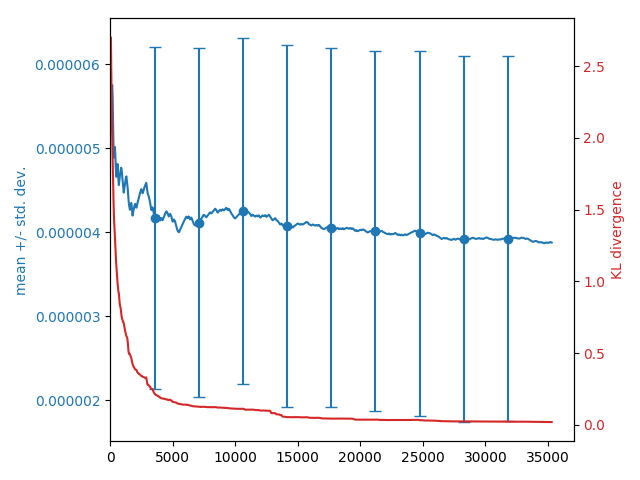
Figure 8: KL divergence (red), and mean and standard deviation (blue), $\texttt{unifCd}(18)$, Schism, 600 seconds

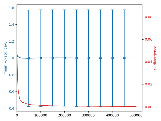
Figure 9: KL divergence (red), and mean and standard deviation (blue), $\texttt{mixed}(5)$, Schism, 600 seconds

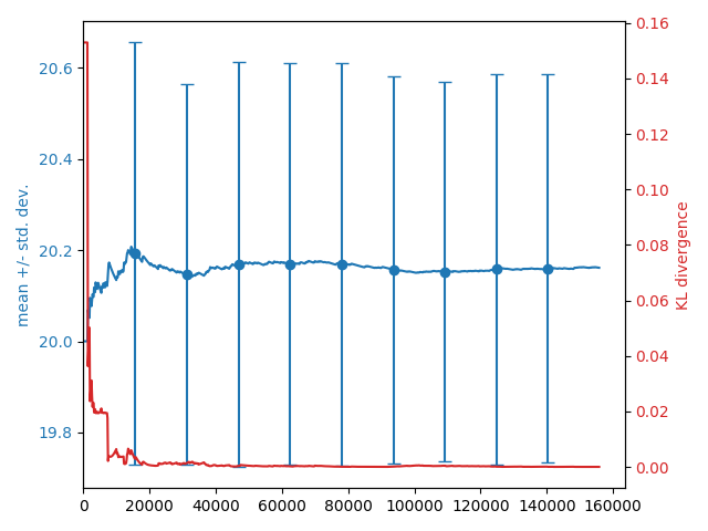
Figure 10: KL divergence (red), and mean and standard deviation (blue), $\texttt{poisCd}(3,20)$, Schism, 600 seconds

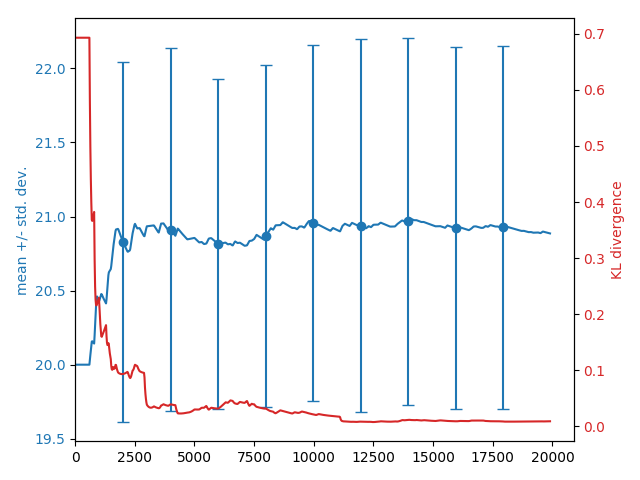
Figure 11: KL divergence (red), and mean and standard deviation (blue), $\texttt{geomIt}(0.5,20)$, Schism, 600 seconds

References

-
[1]
D. Tolpin, J. van de Meent, H. Yang, F. D. Wood,
Design and implementation of
probabilistic programming language Anglican, in: T. Schrijvers (Ed.),
Proceedings of the 28th Symposium on the Implementation and Application of
Functional Programming Languages, IFL 2016, Leuven, Belgium, August 31 -
September 2, 2016, ACM, 2016, pp. 6:1–6:12.
doi:10.1145/3064899.3064910.
URL https://doi.org/10.1145/3064899.3064910 -
[2]
V. K. Mansinghka, D. Selsam, Y. N. Perov,
Venture: a higher-order probabilistic
programming platform with programmable inference, CoRR abs/1404.0099 (2014).
arXiv:1404.0099.
URL http://arxiv.org/abs/1404.0099 -
[3]
B. Carpenter, A. Gelman, M. Hoffman, D. Lee, B. Goodrich, M. Betancourt,
M. Brubaker, J. Guo, P. Li, A. Riddell,
Stan: A probabilistic programming
language, Journal of Statistical Software, Articles 76 (1) (2017) 1–32.
doi:10.18637/jss.v076.i01.
URL https://www.jstatsoft.org/v076/i01 -
[4]
E. Bingham, J. P. Chen, M. Jankowiak, F. Obermeyer, N. Pradhan, T. Karaletsos,
R. Singh, P. A. Szerlip, P. Horsfall, N. D. Goodman,
Pyro: Deep universal
probabilistic programming, J. Mach. Learn. Res. 20 (2019) 28:1–28:6.
URL http://jmlr.org/papers/v20/18-403.html -
[5]
M. F. Cusumano-Towner, F. A. Saad, A. K. Lew, V. K. Mansinghka,
Gen: a general-purpose
probabilistic programming system with programmable inference, in: K. S.
McKinley, K. Fisher (Eds.), Proceedings of the 40th ACM SIGPLAN
Conference on Programming Language Design and Implementation, PLDI 2019,
Phoenix, AZ, USA, June 22-26, 2019, ACM, 2019, pp. 221–236.
doi:10.1145/3314221.3314642.
URL https://doi.org/10.1145/3314221.3314642 -
[6]
T. A. Le, A. G. Baydin, F. Wood,
Inference Compilation and
Universal Probabilistic Programming, in: A. Singh, J. Zhu (Eds.),
Proceedings of the 20th International Conference on Artificial Intelligence
and Statistics, Vol. 54 of Proceedings of Machine Learning Research, PMLR,
Fort Lauderdale, FL, USA, 2017, pp. 1338–1348.
URL http://proceedings.mlr.press/v54/le17a.html -
[7]
D. Tolpin, Deployable
probabilistic programming, in: H. Masuhara, T. Petricek (Eds.), Proceedings
of the 2019 ACM SIGPLAN International Symposium on New Ideas, New
Paradigms, and Reflections on Programming and Software, Onward! 2019, Athens,
Greece, October 23-24, 2019, ACM, 2019, pp. 1–16.
doi:10.1145/3359591.3359727.
URL https://doi.org/10.1145/3359591.3359727 - [8] R. Tsay, R. Chen, Nonlinear Time Series Analysis, Wiley Series in Probability and Statistics, Wiley, 2018.
-
[9]
C. Hur, A. V. Nori, S. K. Rajamani, S. Samuel,
A provably correct
sampler for probabilistic programs, in: P. Harsha, G. Ramalingam (Eds.),
35th IARCS Annual Conference on Foundation of Software Technology and
Theoretical Computer Science, FSTTCS 2015, December 16-18, 2015, Bangalore,
India, Vol. 45 of LIPIcs, Schloss Dagstuhl - Leibniz-Zentrum fuer Informatik,
2015, pp. 475–488.
doi:10.4230/LIPIcs.FSTTCS.2015.475.
URL https://doi.org/10.4230/LIPIcs.FSTTCS.2015.475 - [10] O. Kiselyov, Problems of the lightweight implementation of probabilistic programming, in: proc. ACM SIGPLAN Workshop on Probabilistic Programming Semantics (PPS2016), 2016.
-
[11]
Y. Zhou, H. Yang, Y. W. Teh, T. Rainforth,
Divide, conquer, and
combine: a new inference strategy for probabilistic programs with stochastic
support, in: Proceedings of the 37th International Conference on Machine
Learning, ICML 2020, 13-18 July 2020, Virtual Event, Vol. 119 of
Proceedings of Machine Learning Research, PMLR, 2020, pp. 11534–11545.
URL http://proceedings.mlr.press/v119/zhou20e.html -
[12]
J. van de Meent, B. Paige, H. Yang, F. Wood,
An introduction to probabilistic
programming, CoRR abs/1809.10756 (2018).
arXiv:1809.10756.
URL http://arxiv.org/abs/1809.10756 -
[13]
A. V. Nori, C. Hur, S. K. Rajamani, S. Samuel,
R2: an
efficient MCMC sampler for probabilistic programs, in: C. E. Brodley,
P. Stone (Eds.), Proceedings of the Twenty-Eighth AAAI Conference on
Artificial Intelligence, July 27 -31, 2014, Québec City, Québec,
Canada., AAAI Press, 2014, pp. 2476–2482.
URL http://www.aaai.org/ocs/index.php/AAAI/AAAI14/paper/view/8192 - [14] G. Winskel, The Formal Semantics of Programming Languages, MIT Press, 1993.
-
[15]
L. M. Murray, T. B. Schön,
Automated
learning with a probabilistic programming language: Birch, Annual Reviews in
Control 46 (2018) 29–43.
doi:https://doi.org/10.1016/j.arcontrol.2018.10.013.
URL https://www.sciencedirect.com/science/article/pii/S1367578818301202 -
[16]
F. Olmedo, F. Gretz, N. Jansen, B. L. Kaminski, J. Katoen, A. McIver,
Conditioning in probabilistic
programming, ACM Trans. Program. Lang. Syst. 40 (1) (2018) 4:1–4:50.
doi:10.1145/3156018.
URL http://doi.acm.org/10.1145/3156018 -
[17]
A. D. Gordon, T. A. Henzinger, A. V. Nori, S. K. Rajamani,