Design, construction and validation of an instrumented particle for the lagrangian characterization of flows

Abstract

The design and application of an instrumented particle for the lagrangian characterization of turbulent free-surface flows is presented in this study. This instrumented particle constitutes a local measurement device capable of measuring both its instantaneous 3D translational acceleration and angular velocity components, as well as recording them on an embarked removeable memory card. A lithium-ion-polymer battery provides the instrumented particle with up to 8 hours of autonomous operation. Entirely composed of commercial off-the-shelf electronic components, it features accelerometer and gyroscope sensors with a resolution of 16 bits for each individual axis, and maximum data acquisition rates of 1 and 8 kHz, respectively, as well as several user-programmable dynamic ranges. Its ABS 3D-printed body takes the form of a 36 mm diameter hollow sphere, and has a total mass of $(19.6\pm 0.5)$ g, resulting in an effective mass density of 819 kg/m³, which can be adjusted by incorporating ballasts inside its body. Controlled experiments, carried out to calibrate and validate its performance showed good agreement when compared to reference techniques.

In order to assess the practicality of the instrumented particle, we apply it to the statistical characterization of floater dynamics in experiments of surface wave turbulence. In this feasibility study, we focused our attention on the distribution of acceleration and angular velocity fluctuations as a function of the forcing intensity. The IP’s motion is also simultaneously registered by a 3D particle tracking velocimetry (PTV) system, for the purposes of comparison. Our results show, among other findings, that the IP is able to register the gradual departure from gaussianity and the emergence of strongly non-gaussian distributions for the translational acceleration fluctuations as the forcing amplitude is progressively increased.

Beyond the results particular to this study case, the quality of their agreement with their PTV counterparts and with previous works reported in the literature, constitute a proof of both the feasibility and potentiality of the IP as a tool for the experimental characterization of particle dynamics in such flows.

1 Introduction

In the last two decades, considerable progress has been made in the development of experimental techniques to measure particle transport properties of flows annual_rev_imaging ; Virant_1997 . Most experimental techniques commonly used in the characterization of transport processes in turbulent flows (as is the case of, e.g., particle tracking velocimetry) are based on high speed cameras tracking the trajectory of particles in the flow nature_dudderar_PIV ; Trucco ; MTV . Often, ultra-fast cameras are necessary to extract particle translational accelerations using optical techniques, so as to be able to take multiple derivatives of a registered trajectory at discrete times. Measurement of angular velocities, in turn, also presents considerable experimental challenges 25 ; roco ; 24 ; bordoloi_variano_2017 ; ellen_rotation .

Other families of techniques involve the use of wave sources interacting with seeding particles in the flow. This is the case, e.g., of both imaging laser Doppler velocimetry Imaging_laser_Doppler_velocimetry and ultrasound imaging velocimetry Ultrasound_Imaging_Velocimetry . In contrast, techniques relying on marking lines of fluid particles, such as flow tagging based on the vibrational excitation of oxygen in air flows Miles87 ; Miles89 and molecular tagging velocimetry (MTV) in the case of gas and liquid phase flows koo1993 ; koo1997 ; koo1999 , do not require seeding.

In either case, the implementation of such optic- or sonic-based measurement techniques to characterize flows is impractical in a number of cases, particularly in the situations where the flow is not directly accessible or when the region of interest is large. Such situations are widely present both in the industry and in nature. Some examples of the latter are litter, debris or clusters of algae floating on a large body of water. Industrial applications range from mixing tanks to flows in opaque pipes. In all these scenarios, being able to assess the statistics of particles in the flow represents a substantial advantage, providing valuable information on the transport dynamics of the flow.

For these reasons, alternative measurement techniques involving the use of particles with embedded sensors have been proposed. One of the first implementations of such strategy can probably be traced back to the use of a thermo-sensitive liquid crystal particle in the investigation of heat transfer in fluid flows (see liquidcrystalreview , and references therein). In recent years, gaste2007b employed a particle with a temperature sensor to measure the lagrangian temperature in a Rayleigh-Bénard flow. Later on, smartparticle1 ; smartparticle2 developed a similar device capable of measuring both its own 3D acceleration and temperature. Based on their experimental results, characteristics of the ambient turbulent flow were inferred from the probability density functions of the particle’s translational acceleration and angular velocity bodenschatz1 ; mica1 ; XU20082095 .

In this work we propose the utilization of an enhanced instrumented particle (herein, IP) to characterize particle dynamics in complex laboratory flows. Generally speaking, this IP takes the form of a centimetric-size sphere embarking a 3-axis accelerometer and 3-axis gyroscope, as well as a solid-state storage device; all controlled by a microcontroller unit and powered by a lightweight rechargeable battery. This allows for on-board measuring and recording of the IP’s own translational acceleration and angular velocity. Moreover, the density of the IP can be adjusted to have positive or negative buoyancy.

Being able to simultaneously measure its own acceleration and angular velocity, (closely related to forces and torques) renders the IP an valuable tool for experimental research on the dynamics of inertial particles in turbulent flows, where such quantities play a central role in the development of theoretical models gasteuil ; Bellani421973 ; romain .

In what regards to the particularities of the instrumented particle developed in this study, several aspects are worth highlighting. The first one concerns the electronics embarked in the device. In this respect, the choice was made to build it from commercial off-the-shelf (COTS) components, in order to ensure accessibility and reproducibility, while benefiting from low production costs and open documentation. Indeed, since the advent of the Internet of Things (IoT), a wide variety of sensors based on microelectromechanical systems (MEMS) of relatively high precision and performance have been made available to the public, as is also the case for rechargeable high-capacity power supplies of low mass and reduced volume. As a by-product of this design choice, the inclusion of additional sensors (such as magnetic field, pressure, salinity) is readily available and possible with minor modifications. A second aspect to mention, when compared to preceding developments, is the addition of the gyroscope, which enables the calculation of the non-inertial acceleration terms. Moreover, as the data is stored in a memory card inside the IP, there is no need for external devices acting as data receivers of the particle’s readings. On the other hand, this last feature presents two shortcomings. Including the data logger board imposes a restriction on the minimum diameter of the particle, which in turn introduces a limitation in the scales of the flow the particle is able to resolve. Moreover, as writing data to a non-volatile memory device is a power-intensive operation, the overall power consumption of the system is increased, requiring a larger capacity battery to maintain the same level of autonomy. Secondly, an embarked memory implies that the user must be able to recover the particle after the measurement took place in order to access the data. This might not always be the case, and for this reason the range of applicability of this instrument is mostly limited to laboratory experiments where this is possible.

The structure of the paper is as follows. Section 2 describes the instrumented particle developed for this study, including its electronic components and physical properties. Section 3 regards calibration of the sensors, and Section 4 concerns their validation. An application of the instrumented particle to the characterization of surface wave turbulence is the subject of Section 5. Finally, Section 6 presents our conclusions.

2 Instrumented particle

2.1 Electronic components

The key element of the instrumented particle is the MPU-6050 board (InvenSense Inc.) which integrates, into a single chip, two independently controlled MEMS devices: a 3-axis accelerometer and 3-axis gyroscope mpu6050datasheet . The accelerometer employs separate proof masses for each axis. The mass displacement produced by acceleration along any given axis is detected by capacitive sensors. Three independent vibratory gyroscopes detect rotation about each of the three mutually perpendicular axis. Rotation about an axis induces a vibration (via the Coriolis effect) that is detected by a capacitive pickoff. Both accelerometer and gyroscope signals are amplified and filtered to produce a voltage proportional to the corresponding magnitude. These analog signals are then digitized using six individual on-chip 16-bit ADCs (one for each sensor output channel: 3-axis accelerometer and 3-axis gyroscope). This also enables simultaneous sampling of each signal while requiring no external multiplexer.

Dynamic ranges for the accelerometer and the gyroscope are independently programmable from presets. For the former these ranges are $\pm 2$, $\pm 4$, $\pm 8$, and $\pm 16$ g₀; while for the latter the available ranges are $\pm 250,\pm 500,\pm 1000$, and $\pm 2000\>^{\circ}$/s (i.e., degrees per second), corresponding approximately to $\pm 4.36,\pm 8.73,\pm 17.45,$ and $\pm 34.91$ rad/s. For the accelerometer, the maximum output data rate is 1 kHz, whereas the gyroscope maximum sampling frequency is 8 kHz.

In what regards to power consumption, it is worth mentioning that the accelerometer normal operating current is $500\mu$A, five times lower than that of the gyroscope, rated at 3.6 mA. The MPU-6050 operates with a DC power supply voltage in the range 3.3-5 V.

The results of our preliminary characterization showed that sensing noise for each component of both accelerometer and gyroscope is gaussian distributed, irrespective of the dynamic range. Table 1 presents the noise standard deviation values for the dynamic ranges $\pm 16$ g₀ and $\pm 2000$ ^∘/s; where $a_{i}$ and $\omega_{i}$ represent the translational acceleration and angular velocity, respectively, for the $i$-axis of the corresponding sensor.

Data from the sensors is recorded to a non-volatile memory on-board the particle, by means of an OpenLog data logger (SparkFun Electronics). This board, controlled by its own 16 MHz ATmega328 microprocessor (Atmel Corporation), enables data registering to a removable memory card. It comes preloaded with the Optiboot bootloader which makes it compatible with the Arduino Uno board. This is particularly useful for programming it through the Arduino IDE.

This data logger works over a serial connection and supports standard microSD FAT 16/32 memory cards from 512 Mb up to 32 Gb in storage capacity. Data transfer baud rates are configurable, up to a maximum of 115,200 bps. Our tests showed that the OpenLog draws approximately 5 mA in idle mode and up to 45 mA while recording data to the memory card; moreover, these values vary depending on the size of the microSD card and the baud rate. Lastly, a minimum voltage input of 3.3 V is required to operate the data logger.

Sensor Noise Std Dev	$\hat{x}$	$\hat{y}$	$\hat{z}$
$\sigma(a_{i})$   [g0]	$6.6\times 10^{-3}$	$6.7\times 10^{-3}$	$7.0\times 10^{-3}$
$\sigma(\omega_{i})$   [rad/s]	$2.6\times 10^{-2}$	$2.6\times 10^{-2}$	$4.9\times 10^{-2}$

Table 1: Accelerometer and gyroscope noise standard deviation in units of g₀ and rad/s (respectively) for each of the three axes of the sensors, corresponding to the $\pm 16$ g₀ and $\pm 2000$ ^∘/s dynamic ranges.

In order to automatically control the IP data acquisition and recording, an ATtiny85 chip (Atmel Corporation) is employed as the central processing unit of the IP. This is a 8-bit high-performance, low power AVR^®  CMOS microcontroller with 8 kb in-system programmable flash memory, and a maximum clock speed of 20 MHz attiny85manual . Its power consumption when powered with 3.7 V and operating at the standard 8 MHz frequency (provided by its internal resonator) is approximately 5 mA.

Communication between the microcontroller and its peripherals, namely the sensors and the data logger, is accomplished as follows. The ATtiny85 microcontroller reads the raw data stemming from the MPU-6050 sensors via the I²C (inter-integrated circuit) communication protocol, and passes those values, as well as an associated timestamp, to the OpenLog via a serial connection. The data logger continously records that incoming data stream into a file on the memory card.

Power is supplied by means of a 3.7 V, 150 mAh rechargeable lithium-ion polymer (LiPo) battery model HW651723P. Among those providing sufficient power for this application, this model was chosen due to its low weight (5 g) and relatively small volume ($25\times 16\times 6.5$) mm³. Once fully charged, this power source endows the IP with up to 8 hours of continuous operation.

The electronic connections of the instrumented particle components are presented schematically in Figure 1.

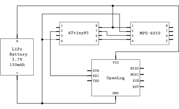
Figure 1: Schematic diagram of the IP’s electronic circuit. The ATtiny85 microcontroller is employed to control both the MPU-6050 sensors (top right) and the OpenLog data logger (bottom right). All three elements are powered by the LiPo battery (to the left of the diagram). Connection points between wires are marked with small black circles.

2.2 Physical properties of the instrumented particle

For the body of the instrumented particle a spherical casing was designed entirely on a 3D CAD parametric modelling software (SOLIDWORKS, Dassault Systèmes). This casing is composed of two hollow spherical caps resulting from cutting a spherical shell along a chord, as seen on Figure 2. The inner side of each cap is designed to hold the IP’s electronic components in predetermined fixed positions (relative to the casing) aimed at homogeneizing the mass distribution inside the IP. Mechanical joining of the two parts is achieved through an internal single-turn equatorial thread. The shell is 3D-printed in an ABS-based production-grade thermoplastic (ABSplus-P430), by means of a Stratasys uPrint SE printer with a layer resolution of 0.254 mm. According to the manufacturer’s specifications, the specific gravity of the material is 1.04.

Within the spherical casing, the sensors are purposedly located at the geometrical center of the particle, which is then made to coincide with its center of mass (to within $\pm 0.5$ mm uncertainty) by means of the addition of appropriately placed ballasts.

The external diameter of the IP is $D_{e}=(36.0\pm 0.1)$ mm; this rather large size is imposed by the dimensions of the electronic component boards and the battery. The total mass of the instrumented particle, determined experimentally, is $m_{\text{IP}}=(19.6\pm 0.5)$ g; in agreement with the estimated 19.41 g arising from the technical specifications of the electronic components and the mass of the shell as calculated via the CAD software (the wires and electric connections, not included in the CAD model, might be the origin of this slight difference). This mass leads to an effective mass density of $\rho_{IP}=819$ kg/m³ for the particle, which can be increased either by modifying the inner geometry of the 3D-printed part or simply by incorporating ballasts inside the shell (e.g., in the form of patches of tungsten conductor paste).

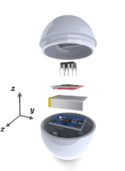
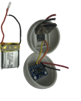
Figure 2: (Left panel) Photorealistic render of the instrumented particle’s components and their internal arrangement. Surrounded by the hollow spherical caps, this diagram shows, from bottom to top: the MPU-6050 (in blue inside the casing), the LiPo battery, the Openlog (in red), and the ATtiny85 chip. The inner sides of the caps feature custom designed slots to keep the electronic components from moving.(Right panel) Photograph of the instrumented particle, prior to final assembly.

The left panel of Figure 2 shows a photorealistic render of the instrumented particle developed in this work, displaying both the IP’s components as well as their internal arrangement. Upon closing the IP by screwing the caps together, the equatorial inner thread forces a 90^∘ rotation on the OpenLog, the plugged memory card, and the ATtiny85, relative to the position shown in this exploded view. This design detail is intentionally introduced to minimize the bias that aligning all electronic components (with their flat and elongated shape) could have on the moments of inertia of the particle. In this schematic representation, connections between components are not shown for the sake of visual simplicity. Complementarily, the right panel of Figure 2 depicts a photograph of the instrumented particle prior to final assembly. In this picture, the inner geometry of the caps is clearly visible, showing the slots designed to keep the electronic components fixed at specific positions inside the particle.

From the 3D CAD design software it is possible to accurately calculate the principal axis of rotation as well as the principal moments of inertia of a given mechanical assembly, provided realistic mass distributions for the individual components are supplied. For the IP, the principal axes of rotation (defined relative to its center of mass) coincide with the accelerometer and gyroscope axes (to within 1% uncertainty). Moreover, the estimated values of the principal moments of inertia of the particle are $J_{x}=1969$ g mm² and $J_{y}=1996$ g mm², for the directions lying on the plane of the equator, and $J_{z}=1897$ g mm² for the perpendicular. The first two differ in less than 1.5%, whereas $J_{z}$ is smaller than its counterparts by a 5% factor.

After the particle is closed and prior to immersing it in the flow, the IP is sprayed uniformly with a peelable rubber coating (Rust-Oleum Peel Coat). This covers the exterior of the particle with a black film of thickness 0.1 mm, providing a waterproof seal for the IP for a minimum lapse of 6 hours. This seal is removeable once the measuring campaign is completed and the particle is opened to recover the memory card holding the acquired data.

Digital design files and Arduino codes are both available upon request from the authors.

2.3 Particle dynamics and sensors’ signals

Due to the IP rotation and the presence of gravity, the acceleration measured by the instrumented particle is not exactly its translational acceleration. In this sense, a time dependent rotation matrix, which represents the instantaneous rotation between laboratory and particle reference frames, is considered. Additionally, centrifugal, Euler and gravity components of acceleration have to be taken into account (note that the Coriolis contribution is null, however, due to the sensor being fixed within the sphere). Hence, the relation between the translational acceleration $\mathbf{a}_{trans}$ and the acceleration $\mathbf{a}_{IP}$ measured by the IP is given by

$$\underline{\underline{\mathbf{R}}}(\mathbf{\alpha}(t))~{}\mathbf{a}_{IP}=\mathbf{a}_{trans}+\mathbf{\omega}\times\big{(}\mathbf{\omega}\times\mathbf{r}\big{)}+\mathbf{\dot{\omega}}\times\mathbf{r}+\mathbf{g}_{0},$$ (1)

where $\mathbf{\omega}$ and $\dot{\mathbf{\omega}}$ are the angular velocity and acceleration, respectively, and $\mathbf{r}$ is the vector defined by the geometric center of the particle and the sensor position. Besides, $\underline{\underline{\mathbf{R}}}(\mathbf{\alpha}(t))$ is the 3D rotation matrix that relates the particle and laboratory reference frames and it depends on the 3D angular position of the particle, $\alpha(t)$. Notice that in the case in which the non-inertial components of the acceleration are negligible and the rotation is isotropic, it is straightforward to relate $a_{trans}$ with $a_{ip}$; whereas in the opposite case it is necessary to make use of the angular velocity measurements to derive those contributions. In either case, it is possible to calculate even central moments of $a_{trans}$ ZimmermannThesis .

3 Calibration

The 3D accelerometer requires a calibration to obtain its offset and sensitivity. The procedure of calibration is based on the fact that if the sensor is at rest, the norm of the measurements must be equal to the local acceleration of gravity:

$$\left(\frac{A_{x}-O_{x}}{S_{x}}\right)^{2}+\left(\frac{A_{y}-O_{y}}{S_{y}}\right)^{2}+\left(\frac{A_{z}-O_{z}}{S_{z}}\right)^{2}=\text{g}_{0}^{2},$$ (2)

where the vectors $\mathbf{O}=(O_{x},O_{y},O_{z})$ and $\mathbf{S}=(S_{x},S_{y},S_{z})$ are the sensor’s offset and sensitivity; respectively, and the raw accelerometer readings in each direction are represented by $\mathbf{A}=(A_{x},A_{y},A_{z})$. In order to obtain $\mathbf{O}$ and $\mathbf{S}$ from this equation, the following procedure is carried out. Time series of raw 3D-acceleration data are acquired for 9 mutually independent orientations of the sensor (parallel and antiparallel to gravity for the three proper axes, plus three arbitrary orientations) while at rest. For each instantaneous determination of the 9 raw acceleration time-series, eq. (2) results in a system of equations that can be solved to obtain the values of sensitivity and offset for each axis. In all cases, we employed time-series data consisting of 10,000 data points (corresponding to a 10 s acquisition lapse at the maximum sampling frequency) for each orientation; obtaining an equal number of determinations of $\mathbf{O}$ and $\mathbf{S}$.

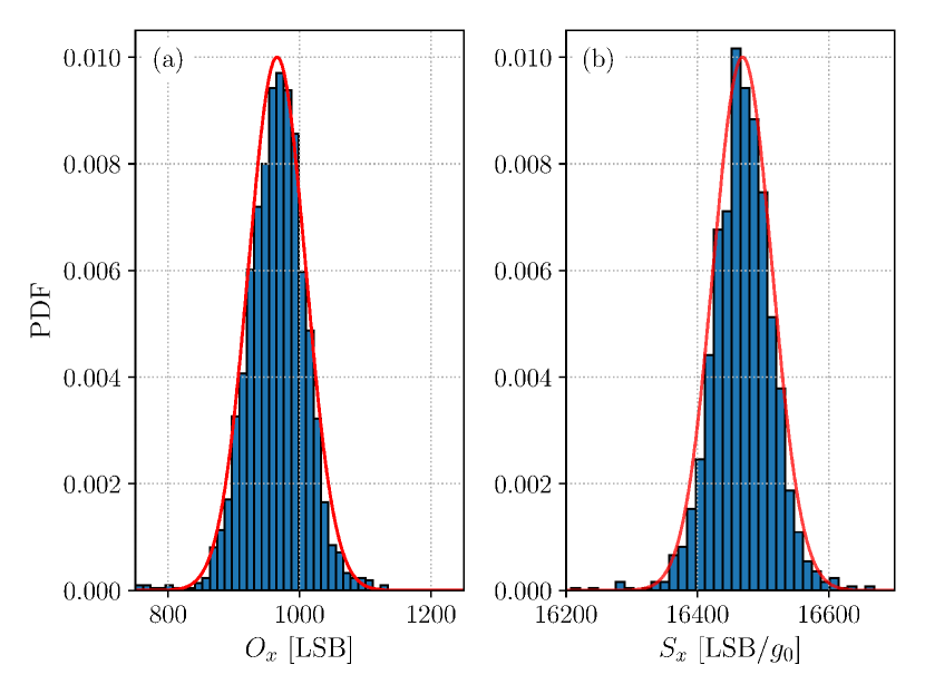
Figure 3: Distributions for offset (left panel) and sensitivity (right panel) derived from the accelerometer calibration described in the text. Results are only shown here for the $x$-axis and $\pm 2$ g₀; qualitatively similar behaviors were obtained for other axes and dynamic ranges. In both panels, a fit by a gaussian distribution is represented by a (red) continuous line.

Our results show that both offset and sensitivity are gaussian distributed; we therefore define their values as those resulting from their distribution means. As an illustration, panels (a) and (b) of Figure 3 present these calibration results for the offset and sensitivity distributions for one particular axis of the MPU-6050 accelerometer operating at the $\pm 2$ g₀ dynamic range, respectively. Note that the mean sensitivity value obtained is comparable with an estimate based on the ratio of the maximum representable integer at the board’s bit resolution and the working dynamic range; namely: $S=2^{16}/4$ g₀ = 16,384 in units of LSB/g₀, where LSB stands for Least Significant Bit.

As the values for offset and sensitivity depend also on the overall dynamic range chosen for the sensor, this calibration procedure was repeated for each of them. Qualitatively similar behaviors were observed for other axes and dynamic ranges.

Finally, in the case of the gyroscope, the corresponding values for offset and sensitivity were taken from the MPU-6050 datasheet and successfully validated in the following Section.

4 Validation

4.1 Gyroscope validation

The gyroscope performance is validated according to the following procedure. The particle is mounted at the end of a rotating DC motor’s shaft, making sure the selected sensor axis is properly aligned with it. This can accomplished by setting the motor in motion, monitoring the signals read by the remaining two axes for coherent signals (corresponding to projections of the angular velocity) and correcting for misalignment. Once the axis is aligned, the motor is made to rotate at a controlled angular frequency while acquiring a time series signal of the IP’s angular velocity. This operation is repeated for several rotation frequencies between $0.3$ and $1.2$ rad/s (limited by the geared motor employed), and for the three axes of rotation of the gyroscope.

The results of this validation are presented in Figure 4, for each of the gyroscope axes, along with a dashed line of slope equal to unity, included as a visual reference. In the Figure, horizontal error bars are associated with the uncertainty in the imposed frequency, whereas vertical error bars result from the standard deviation of each time series.

Although the specific values for each axis differ slightly, separate linear fits (not shown in the figure) result in slopes ranging from 0.971 to 1.018, and absolute values for the corresponding intercepts lower than 0.005 (both established with an uncertainty of 1.5%).

Our results are compatible with the values reported in the sensor’s documentation, therefore in what follows we employ those values for the offset and sensitivity of the gyroscope.

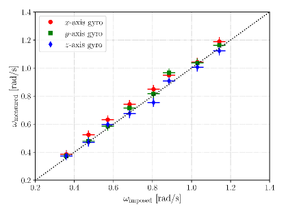
Figure 4: Results for the validation of the instrumented particle’s gyroscope. Data for the $x$, $y$, and $z$ axis is represented by (red) circles, (green) squares, and (blue) diamonds, respectively. A dashed (black) line of slope equal to unity is displayed as a visual reference.

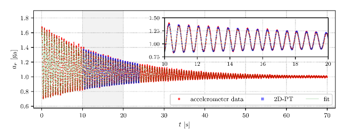
Figure 5: Accelerometer validation results through a physical pendulum experiment. Measurements of the IP’s sensor radial acceleration, shown in (red) circles, are compared to: (a) its counterparts obtained from PTV, depicted by (blue) squares and only available within a reduced time window, and (b) the best-fit based on an approximate theoretical prediction, represented by a continuous (green) line. The inset shows a zoomed view of the three curves in the region highlighted by a gray background.

4.2 Accelerometer validation

For this validation, the sensor is mounted at the tip of a physical compound pendulum consisting of a thin, stiff rod and a mass attached to its end; capable of swinging about a pivot point by means of a ball bearing. During the oscillating motion, the sensor records its acceleration while a fast camera simultaneously captures the 2D movement of the pendulum. Particle tracking is employed later to determine the trajectory of the pendulum, from which the radial acceleration registered by the sensor can be extracted.

For the acceleration measurements, the accelerometer was set at a sampling frequency of 100 Hz, and the $\pm 2$ g₀ dynamic range was selected. For particle tracking, the images were acquired by a Photron Fastcam SA3-60K camera ($1024\times 1024$ px² resolution, 12-bits color depth). The image sampling rate was established at $50$ Hz (lowest available value for this setting on the camera) and a shutter speed of $1/1000$ s was chosen to minimize the effects of motion blur on particle tracking. The resulting error in position tracking was estimated (a posteriori) to be better than 0.5%. Due to limitations in the amount of flash memory available, the camera is only able to record for approximately 25 s during the pendulum motion.

Accelerometer results are also compared to the theoretical prediction for the radial acceleration as registered by the sensor, given by

$$a_{r}(t)=r\omega^{2}\theta_{0}^{2}e^{-2\gamma t}\sin^{2}(\omega t)+g_{0}\cos[\theta_{0}e^{-\gamma t}\cos(\omega t)],$$ (3)

where $r$ is the distance between the pivot and the position of the sensor, $\theta_{0}$ is the initial angle of the motion, $\gamma$ is the damping factor and $\omega$ is the oscillation frequency, given by $\omega^{2}=\omega^{2}_{0}-\gamma^{2}$; $\omega^{2}_{0}$ being the natural frequency of the undamped pendulum. It is worth mentioning that equation (3), derived in articulo_pendulo , is valid for small damping ($\gamma\ll\omega$) and under the small angle approximation ($\theta_{0}\ll\pi/2$).

Figure 5 shows the results for the radial acceleration measured by the sensor (in red circles) for a time lapse of 70 s which covers the dynamics from the pendulum’s release up to its equilibrium state. These results are compared to those derived from the 2D particle tracking algorithm (in blue squares) available for a narrower time window corresponding to $t\in[10,24]$ s. A good agreement is observed between the accelerometer data and the results from particle tracking in this overlapping zone.

Additionally, parameters of the model equation (3) are adjusted to our accelerometer data; the results from this fit are represented as a continuous (green) line in the same Figure. The best-fit values obtained for the parameters are as follows: $\omega=5.23$ rad/s, comparable to the theoretical value of 5.8 rad/s based on an estimate for the inertia moment of the pendulum; $r=0.37$ m, close to the pendulum’s length of 0.39 m; the damping factor value $\gamma=0.02$ s^-1, compatible with a low damping regime; and $\theta_{0}=0.78$ rad, in agreement with the initial angular displacement (of approximately 45^∘) imposed on the pendulum.

Comparison between the accelerometer data and the theoretical prediction reveals again good agreement over the entire motion, both in terms of the frequency of oscillation and the upper and lower amplitude envelopes. The inset in Figure 5 displays a zoomed view of these three signals (accelerometer data, 2D-PT, and theoretical prediction) in the time interval highlighted with a gray background (where they coexist), showing a three-fold agreement.

This validation procedure was repeated by changing the axis of the accelerometer pointing in the radial direction, leading to results similar to those presented in the preceding paragraphs (omitted in this exposition for the sake of brevity).

5 Application to surface wave turbulence

This section presents the results of the application of a buoyant version of our IP to characterize a free-surface wave turbulence flow. Typical results of the statistical properties of acceleration and angular velocity are analyzed. The goal is to use these results of the IP dynamics in a known flow as a benchmark for the performance of the instrumented particle and its applicability to the characterization of flows.

5.1 Experimental setup

Figure 6 presents a schematic representation of the experimental setup employed in this Section. The experiments are carried out in a PMMA wave tank of dimensions (2.0$\times$0.8$\times$ 0.15) m³. Distilled water is employed as the working fluid, with the addition of TiO₂ powder in a low concentration (4 g/l) in order to render the liquid white without significantly changing its rheological properties Przadka2012 . This simplifies the detection and subsequent tracking of the particle for the PTV measurements since a strong color contrast is achieved between the (black) IP and the surrounding (white) fluid in which it is partially immersed.

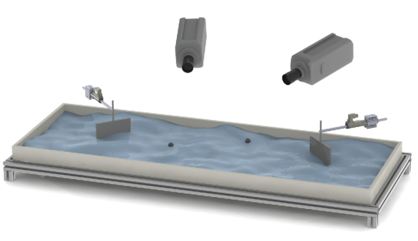
Figure 6: Schematic diagram of the experimental setup employed in the study of floater dynamics in surface wave turbulence. Waves are created by the stirring motion of paddles, independently controlled by servo-motors (see text for details on the forcing characteristics). Two identical instrumented particles are used, together with a 3D-PTV system composed of two high-speed cameras.

A turbulent steady state of surface waves is generated (and sustained) by continuously stirring the flow with two partially immersed paddles. The piston-type motion of these paddles, whose surface area is (15$\times$10) cm², is established by two independently-driven servo-controlled electromagnetic linear motors (LinMot, model P01-23$\times$80/210$\times$270) with a peak force of 47 N and a position accuracy of 0.01 mm. These wavemakers were driven by a random signal with a white frequency spectrum in the range [0, 4] Hz (as done in experiments of gravity wave turbulence; see, for instance, in Cobelli2011 ; delgrosso2019 ). According to this, the signal used for the forcing thus naturally determines a characteristic time scale of approximately 0.25 s. As the tank is filled with liquid up to a height at rest $h_{0}=5$ cm, this forcing leads to waves in the deep water regime, following a dispersion relation approximately given by $\omega^{2}\approx g_{0}k\tanh(kh_{0})$, where $k$ represents the wave number.

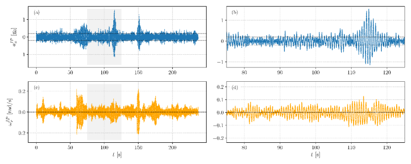
Figure 7: Translational acceleration (top row) and angular velocity (bottom row) time series as measured by the instrumented particle in the experiments on gravity wave turbulence, acquired at a sampling frequency of 100 Hz for a forcing amplitude of $A=15$ mm. Only the $x$ component is shown, qualitatively similar behaviors were registered for the remaining axes. Panels (b) and (d) show a zoomed view of the time series depicted in panels (a) and (c), respectively; within the 50 s time window highlighted in gray. RMS values for $a^{IP}_{x}(t)$ and $\omega_{x}^{IP}(t)$ are marked in the panels by a dotted (black) line.

The same maximum amplitude for the wavemakers’ motion, symbolized by $A$, was imposed for to both paddles; its value was then varied for different experimental runs. For this study, experiments with four different values of the maximum forcing amplitude $A$ were considered, namely: 5, 10, 15 and 20 mm. This choice allows for the exploration of regimes with different levels of nonlinear coupling between waves. It is worth noting that the amplitude $A$ corresponds to the maximum amplitude for the displacement of the paddle as measured from its position at rest. Due to the fact that random time signals were employed for the forcing, the actual mean displacements of the wavemakers were smaller (e.g., for $A=10$ mm, the associated standard deviation of the paddle’s position from rest is 2.7 mm).

In order to track the IP during its motion in the turbulent wave field, a 3D PTV system was implemented employing two high-speed Photron cameras (a SA-3 camera and a 1024-PCI camera) whose complete field of view covers the entire wave tank. Calibration results, following the procedure described by zhang1999 , resulted in an position uncertainty of 0.3 mm. For both cameras, the acquisition frequency and shutter speed were set at 60 Hz and 1/250 s, respectively; synchronicity was achieved by means of an external trigger.

The experimental protocol is as follows. At first, the wavemakers are set in motion from an initially rest state. After a transient period (of 3–5 min) in which a steady state is established, two identical IPs are placed in the turbulent wave field. For the instrumented particles, the acquisition frequency for both the embarked accelerometer and gyroscope was set at 100 Hz; whereas the dynamic ranges chosen for each sensor (based on preliminary tests) are $\pm 4$ g and $\pm 250^{\circ}$/s, respectively. Once the cameras’ recording time is elapsed, and during the time period in which images are uploaded to an external device for storage, the forcing is maintained and the IPs continue to register data, leading to acceleration and angular velocity time series of a typical duration of 240 s.

It is worth mentioning that the experimental runs considered for this study do not include particle collisions (with either the paddles, the wave tank walls or between each other). Moreover, a posteriori analysis of the PTV results revealed that, for those selected cases, the distance between the two IPs remained always greater than 5 (particle) diameters.

Each experimental run consisted of approximately 40 s of simultaneous IP and PTV measurement, plus an extended period of 200 s in which only IP data is gathered. Furthermore, a total of 5 identical (repeated) experiments were carried out for each value of the maximum forcing amplitude $A$ explored, resulting in a total of 20 experimental realizations.

For the particles, 3D data on translational acceleration and angular velocity is gathered for each experiment. Typical time series for these magnitudes are shown in Figure 7, corresponding to one particular axis (arbitrarily chosen, as qualitatively similar results are obtained for other axes). Panel (a) displays the translational acceleration $a_{x}$ whereas panel (c) depicts the angular velocity $\omega_{x}$, both for the same experimental run, which corresponds to a forcing amplitude value of $A=15$ mm. Panels (b) and (d) display a zoomed view of the corresponding signal in the time window highlighted in gray (i.e., between 75 and 100 s). RMS values for these signals are marked in the panels by a dotted black line. Notice that, with peak absolute values slightly exceeding 1 g₀ in the case of the accelerometer and 0.2 rad/s for the gyroscope, both sensors are still far from saturation.

The accelerometer signals exhibit relatively long lapses of random fluctuations about a null mean, whose amplitude coincide with the RMS value (which in this case is 0.19 g₀), separated by short-timed intense bursts such as those occurring at $t\approx 115$ s and $t\approx 150$ s, in which the acceleration reaches values of order 1 g₀. These events point towards the emergence of sudden and localized variations of the free-surface state at the particle’s instantaneous position, and are associated to dissipative mechanisms in the flow, such as the formation of cusps and wave breaking.

A similar behavior is observed in the case of the signals registered by the gyroscope, as seen on Figure 7(c). Moreover, comparison between panels (a) and (c) shows some degree of correlation between $a_{x}(t)$ and $\omega_{x}(t)$ for intense events, although this is not always the case (notice, e.g., the burst in angular velocity occurring at $t\approx 175$ s, with no significant trace in the acceleration time series).

Finally, both the acceleration and angular velocity time series reveal the presence of a carrier frequency of approximately 1.67 Hz, made evident in the zoomed view of panels (b) and (d). This frequency corresponds (roughly) to the center of the frequency band of the forcing signal, and therefore appears naturally in the IP signals.

Particle tracking, on the other hand, allows for the determination of individual particle trajectories from which acceleration can be calculated and compared to IP data. In our data post-processing scheme, acceleration is derived by fitting a series of cubic splines in a piecewise manner to the discrete positions of the particles at discrete instants in time. This implies that third order polynomials are fitted between discrete time points, therefore ensuring continuity of velocity and acceleration. As no synchronization between the cameras and the particles is enforced, the comparison between IP data and results from PTV is carried out in terms of the statistical properties of their distributions.

Since the instrumented particle has a finite size, the physical scales to which it is sensitive in the flow under study is naturally limited. Therefore, in order to draw conclusions on the dynamics observed, it is important to estimate the minimum size of flow structures (such as waves, in this scenario) the IP is able to resolve.

In order to derive an estimate for this spatial scale, we proceed as follows. First, the scaling law for the gravity wave turbulence power spectrum (theoretically predicted and experimentally observed in Cobelli2011 ) is considered: $P(f)\propto\omega^{-17/6}$, where $P$ is the power spectral density and $\omega$ the (angular) frequency of the waves. The smaller scales injected in the turbulent wave field are associated to the maximum frequency of forcing; corresponding, in this case, to $\omega_{f}=(2\pi\cdot 4)$ rad/s, as we employ forcing frequencies in the 0–4 Hz range. Next, a cutoff frequency whose power is an order of magnitude less than the power injected into the flow, is estimated. This cutoff frequency $\omega_{c}$, obtained from the aforementioned condition given by $P(\omega_{c})=0.1\>P(\omega_{f})$, leads to $\omega_{c}\approx 56$ rad/s. By inverting the dispersion relation for gravity waves, the associated wave number is calculated, from which a characteristic scale can be derived. This is found to be approximately 2 cm, comparable in order of magnitude with the size of the particle. For the angular frequency, the corresponding value for the cut-off is smaller (by a factor of 2) than the frequency of transition between the gravity and capillary wave turbulence regimes, as established in FalconSIAM . In summary, the instrumented particle is sensitive, essentially, to the full range of surface gravity waves.

5.2 Angular velocity fluctuations

Angular velocity fluctuations follow a normal distribution, as evidenced from the associated normalized probability density function (PDF) shown in Figure 8 for the case of the most intense forcing ($A=20$ mm). No significant difference between the readings of the three axes is observed, and qualitatively comparable results are obtained for the other forcing levels considered in this study. Note that although the tails of the distribution separate from the normal distribution (depicted by a dotted black line in the Figure), their point density is significantly lower than that of the central region.

In order to quantify the gaussian behavior of the PDFs, a one-sample Kolmogorov-Smirnov test is performed, testing the null hyphothesis that the data is drawn from a gaussian distribution (whose mean and standard deviation are data driven). Our results show that, as anticipated by the PDFs, the distributions for the angular velocity fluctuations are indeed gaussian distributed, with $p$-values below $3\times 10^{-1}$.

Moreover, from this analysis it is observed that the particles’ mean angular velocities (for all axes and forcing intensities) adopt values of the order of $1.6\times 10^{-6}$ rad/s, lower than the noise level of $5.5\times 10^{-2}$ rad/s; with RMS values of $4\times 10^{-2}$ rad/s that are above the sensitivity (which, for this dynamic range, is $1\times 10^{-3}$ rad s^-1 LSB^-1). Peak values for the IP’s angular velocity are, in all cases explored, lower than 0.26 rad/s.

As can be seen from panels (c) and (d) in Figure 7, the particle rotates about a given axis with alternating positive and negative velocity, with a periodicity linked to the characteristics of the underlying flow (recall that the wave field is generated by forcing at time-scales within the 0–4 Hz band).

Based on these results, and taking into account the 0.5 mm uncertainty in the placement of the sensors relative to the particle’s center, an order-of-magnitude estimate can be given for the non-inertial contributions in eq. (1) in terms of the maximum angular velocity and acceleration. According to this, $|\mathbf{a}_{cen}|\approx 2.2\times 10^{-4}$ m/s² and $|\mathbf{a}_{eul}|\approx 8\times 10^{-4}$ m/s².

5.3 Translational acceleration fluctuations

In this subsection the IPs’ translational acceleration fluctuations are considered. Our experimental results for these magnitudes are summarized in Figure 9. Panels (a) through (d) show the normalized probability density functions for each of the three components of translational acceleration in increasing order of the forcing amplitude $A$. Results obtained from the instrumented particles are represented by squares, while those derived from the particle tracking technique are depicted with a star; each acceleration component being color-coded so that red, green, and blue denote the $x$, $y$, and $z$ axes, respectively. For comparison purposes, each panel comprises also a standard normal distribution, represented by a dotted black line.

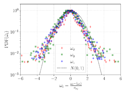
Figure 8: Probability density functions of the (normalized) angular velocity registered by the instrumented particle for the largest forcing amplitude considered ($A=20$ mm). Data is shown with markers: (red) diamonds, (green) squares and (blue) stars denote the $x$, $y$, and $z$ axes, respectively. A standard normal distribution is depicted by a (black) dashed line, as a reference.

As seen in the previous subsection, the two non-inertial components of the acceleration measured by the particle have maximum values below $1\times 10^{-3}$ m/s², while the measured values of acceleration are of order 1 g₀ (i.e., 9.8 m/s²). Therefore, rotational contributions to the acceleration in equation (1) can be neglected, leading to the following simplified form:

$$\mathbf{\underline{\underline{R}}\mathbf{(\alpha(t))}}\>\mathbf{a}_{ip}=\mathbf{a}_{trans}+\mathbf{g}_{0}.$$ (4)

As previously discussed, accelerometer and PTV reference systems are related by a time dependent transformation hence their axes have generally different orientations. Due to the fact that the three accelerometer axes sweep the space homogeneously, we expect the acceleration distribution to be similar for each sensor axis, which is compatible to the results shown in Figure 9.

The good agreement found between the results independently obtained from the instrumented particle and the particle tracking technique contitutes a positive result indicating the feasibility of application of the IP to characterize this type of turbulent flows.

Finally, it is worth considering how the translational acceleration fluctuation distribution is modified as the forcing is increased. In this sense, Figure 9 shows a PDF behavior close to gaussian only for the lowest forcing (top left panel, corresponding to $A=5$ mm). As the forcing is increased beyond that value, the experimental data gradually departs from the normal distribution and begins to exhibit progressively heavier exponential tails (and consequently, sharper maxima). This is particularly evident in the last panel (bottom right, associated to $A=20$ mm, the most intense forcing considered), where our experimental results show a clearly non-gaussian behavior. Concurrently, we observe a monotonous growth on the standard deviation of acceleration fluctuations as the injected power increases.

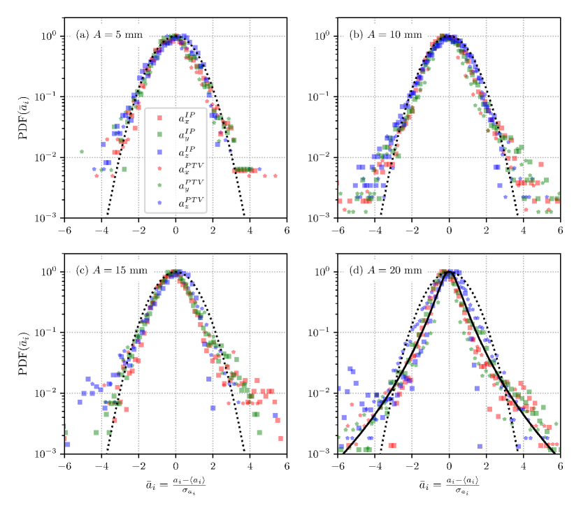
Figure 9: Probability density functions of the (normalized) translational acceleration of the instrumented particle, for increasing values of the forcing amplitude. Data from the instrumented particle and from 3D-PTV is represented by squares and stars, respectively. Red, green and blue are employed to denote the $x$, $y$, and $z$ axes, in that order. A standard normal distribution is depicted by a (black) dashed line, as a reference. Additionally, a stretched exponential distribution corresponding to $\Pi_{s}(a^{IP}_{x})$ as defined by eq. (5), is displayed in panel (d) by a continuous (black) line.

These results are in agreement with previous experimental studies on other turbulent flows 11 ; 55 ; 54 ; 72 . In those works, the normalized distribution for the acceleration $a_{i}$ along a given $i$-axis is modeled by:

$$\Pi_{s}(a_{i})=\frac{e^{3s^{2}/2}}{4\sqrt{3}}\left[1-\text{erf}\left(\frac{\ln|a_{i}/\sqrt{3}|+2s^{2}}{s\sqrt{2}}\right)\right],$$ (5)

where the value of the parameter $s$ is related to the data kurtosis, $\kappa$, through the expression:

$$\quad s=\frac{1}{2}\sqrt{\ln\left(\frac{5}{9}\>\kappa\right)}.$$ (6)

The model given by eq. (5) is extensively employed in the analysis of intermittency in the dynamics of particles (see, for instance, 45 and references therein) and arises from from the approximation that the norm of the acceleration presents a log-normal distribution.

In Figure 9(d) the function $\Pi_{s}(a^{IP}_{x})$ is plotted in a black continuous line, for a value of $s=0.4$ corresponding to a kurtosis of $\kappa=3.41$ as determined experimentally from the instrumented particle data. It is observed that, without adjustable parameter, a stretched exponential describes adequately our experimental results for the distribution of acceleration fluctuations. Although not shown in the Figure, we verified that this result holds also for the data shown in panels (b) and (c), i.e. for $A=10$ mm and $A=15$ mm, respectively. This non-gaussianity of the acceleration components is a manifestation of intermittency in turbulence, which is known to have direct consequences on the forces exerted by the flow on an inertial particle 21 .

6 Conclusions

An instrumented particle for the characterization of turbulent flows is presented in this study. This device takes the form of a 36 mm sphere. It constitutes an autonomous local measurement device capable of measuring both its translational acceleration and angular velocity components employing a high acquisition rate (up to values of the order of the kHz), as well as recording them on an embarked microSD removeable memory card. A LiPo battery powers the electronics, providing the particle with up to 8 hours of autonomous operation. Its sensors have a resolution of 16 bits, and maximum acquisition frequencies of 1 kHz for the accelerometer and 8 kHz for the gyroscope; as well as various user-programmable dynamic ranges. This instrumented particle has a total mass of slightly less than 20 g, resulting in an effective mass density of 819 kg/m³. Moreover, this density can be increased (within certain limits) by the inclusion of properly dimensioned ballasts inside the sphere.

It is worth pointing out that all the IP’s electronic components are COTS (commercial off-the-shelf), thereby presenting considerable advantages, such as easy accessibility, low comparative cost, seamless upgrading and open documentation.

The particle’s design and its properties, ranging from the choice of electronic components to the construction of the casing and its assembly, is discussed in detail. A calibration protocol is established and the IP’s sensors are validated through two controlled experiments. For the 3-axis accelerometer, in particular, this validation stage shows very good agreement between the signals measured by the IP, those obtained by a particle tracking technique and a theoretical prediction.

Finally, the last Section presents an application of the IP to the statistical characterization of a turbulent flow. For this purpose we choose a surface wave turbulence scenario, generated in a water-filled wave tank by the stirring motion of piston-type wavemakers. A steady turbulent wave field of controlled characteristics is created by forcing the wavemakers with a white-noise random signal of amplitude $A$ within the 0–4 Hz frequency band. In order to explore the effect of the energy injection on the flow, four different forcing amplitudes are considered.

This turbulent flow is then studied simultaneously with our instrumented particle (two identical IPs are used in this case, actually) and their movement is also registered by a 3D-PTV system for the purposes of comparison.

Both measurement methods (IP and PTV) resulted in similar translational acceleration statistical behavior, for all axes and forcing intensities. The statistics of translational acceleration fluctuations measured by the IP as a function of the forcing amplitude reveal the departure from gaussianity and the emergence of strongly non-gaussian distributions, indicated by heavy tails beyond three standard deviations and sub-normal behavior around the mean value. These results are in qualitative agreement with previous studies carried out in other turbulent systems. Additionally, it is shown that, by using a stretched exponential distribution (with no adjustable parameters) it is possible to adequately describe the non-gaussian behavior observed for the acceleration PDFs. The non-gaussianity of these distributions accounts for the intermittency in the flow, and the action of forces much higher than the average with occurrence rates above what is expected for a normal distribution. Additionally, the angular velocity of the particles was studied. Temporal angular velocity measurements coming solely from the instrumented particle present, in contrast, gaussian distributed fluctuations.

Beyond the particularities inherent to this chosen case study, the results drawn from the application of the IP to a free-surface turbulent flow and, more importantly, the quality of their agreement with their PTV counterparts and with previous works in similar physical scenarios, constitute a proof of both the feasibility and potentiality of using the IP for the characterization of particle dynamics in such flows.

- [1] R. J. Adrian. Particle-imaging techniques for experimental fluid mechanics. Annual Review of Fluid Mechanics, 23(1):261–304, 1991.
- [2] M. Virant and T. Dracos. 3d PTV and its application on lagrangian motion. Measurement Science and Technology, 8(12):1539–1552, dec 1997.
- [3] T. D. Dudderar and P. G. Simpkins. Laser speckle photography in a fluid medium. Nature, 270(5632):45–47, 1977.
- [4] E. Trucco and A. Verri. Introductory Techniques for 3-D Computer Vision. Prentice Hall PTR, Upper Saddle River, NJ, USA, 1998.
- [5] B. Stier and M. M. Koochesfahani. Molecular tagging velocimetry (mtv) measurements in gas phase flows. Experiments in Fluids, 26(4):297–304, 1999.
- [6] Michael B. Frish and Watt W. Webb. Direct measurement of vorticity by optical probe. Journal of Fluid Mechanics, 107:173–200, 1981.
- [7] J. Ye and M. C. Roco. Particle rotation in a couette flow. Physics of Fluids A: Fluid Dynamics, 4(2):220–224, 1992.
- [8] S. Klein, M. Gibert, A. Bérut, and E. Bodenschatz. Simultaneous 3d measurement of the translation and rotation of finite-size particles and the flow field in a fully developed turbulent water flow. Measurement Science and Technology, 24(2):024006, dec 2012.
- [9] A. D. Bordoloi and E. Variano. Rotational kinematics of large cylindrical particles in turbulence. Journal of Fluid Mechanics, 815:199–222, 2017.
- [10] D. Barros, B. Hiltbrand, and E. K. Longmire. Measurement of the translation and rotation of a sphere in fluid flow. Experiments in Fluids, 59(6):104, 2018.
- [11] A. H. Meier and T. Roesgen. Imaging laser doppler velocimetry. Experiments in Fluids, 52(4):1017–1026, 2012.
- [12] C. Poelma. Ultrasound imaging velocimetry: a review. Experiments in Fluids, 58(1):3, 2016.
- [13] R. Miles, C. Cohen, J. Connors, P. Howard, S. Huang, E. Markovitz, and G. Russell. Velocity measurements by vibrational tagging and fluorescent probing of oxygen. Opt. Lett., 12(11):861–863, Nov 1987.
- [14] R. B. Miles, J. J. Connors, E. C. Markovitz, P. J. Howard, and G. J. Roth. Instantaneous profiles and turbulence statistics of supersonic free shear layers by raman excitation plus laser-induced electronic fluorescence (relief) velocity tagging of oxygen. Experiments in Fluids, 8:17–24, 1989.
- [15] MM Koochesfahani, CP Gendrich, and DG Nocera. A new technique for studying the lagrangian evolution of mixing interfaces in water flows. Bull Am Phys Soc, 38:2287, 1993.
- [16] CP Gendrich, MM Koochesfahani, and DG Nocera. Molecular tagging velocimetry and other novel applications of a new phosphorescent supramolecule. Experiments in Fluids, 23:361—372, 1997.
- [17] B. Stier and M. Koochesfahani. Molecular tagging velocimetry (mtv) measurements in gas phase flows. Experiments in Fluids, 26:297–304, 1999.
- [18] J. W. Baughn. Liquid crystal methods for studying turbulent heat transfer. International Journal of Heat and Fluid Flow, 16(5):365 – 375, 1995.
- [19] W. L. Shew, Y. Gasteuil, M. Gibert, P. Metz, and J.-F. Pinton. Instrumented tracer for lagrangian measurements in rayleigh-bénard convection. Review of Scientific Instruments, 78(6):065105, 2007.
- [20] R. Zimmermann, L. Fiabane, Y. Gasteuil, R. Volk, and J.-F. Pinton. Measuring lagrangian accelerations using an instrumented particle. Physica Scripta, T155, 06 2012.
- [21] R. Zimmermann, L. Fiabane, Y. Gasteuil, R. Volk, and J.-F. Pinton. Characterizing flows with an instrumented particle measuring lagrangian accelerations. New Journal of Physics, 15(1):015018, jan 2013.
- [22] S. Ayyalasomayajula, A. Gylfason, L. R. Collins, E. Bodenschatz, and Z. Warhaft. Lagrangian measurements of inertial particle accelerations in grid generated wind tunnel turbulence. Phys. Rev. Lett., 97:144507, Oct 2006.
- [23] N. M. Qureshi, U. Arrieta, C. Baudet, A. Cartellier, Y. Gagne, and M. Bourgoin. Acceleration statistics of inertial particles in turbulent flow. The European Physical Journal B, 66(4):531–536, 2008.
- [24] H. Xu and E. Bodenschatz. Motion of inertial particles with size larger than kolmogorov scale in turbulent flows. Physica D: Nonlinear Phenomena, 237(14):2095 – 2100, 2008. Euler Equations: 250 Years On.
- [25] R. Zimmermann, Y. Gasteuil, M. Bourgoin, R. Volk, A. Pumir, and J.-F. Pinton. Rotational intermittency and turbulence induced lift experienced by large particles in a turbulent flow. Phys. Rev. Lett., 106:154501, Apr 2011.
- [26] G. Bellani, A. Collignon, and E. A. Variano. Turbulence modulation and rotational dynamics of large nearly neutrally buoyant particles in homogeneous isotropic turbulence. Technical report, KTH, Linné Flow Center, FLOW, 2012. QC 20110610.
- [27] N. Machicoane and R. Volk. Lagrangian velocity and acceleration correlations of large inertial particles in a closed turbulent flow. Physics of Fluids, 28(3):035113, 2016.
- [28] InvenSense. MPU-6000 and MPU-6050 Product Specification. InvenSense Inc., California, USA, 9 2013. Document No.: PS-MPU-6000A-00, Revision 3.4.
- [29] Atmel. Atmel 8-bit AVR Microcontroller with 2/4/8 kBytes In-System Programmable Flash. Atmel Corporation, California, USA, 8 2013. Rev. 2586Q-AVR.
- [30] R. Zimmermann. How large spheres spin and move in turbulent flows. PhD thesis, École Normale Supérieure de Lyon, Université de Lyon, Lyon, France, 7 2012.
- [31] C. Dauphin and F. Bouquet. Physical pendulum experiment re-investigated with an accelerometer sensor. Papers in Physics, 10:100008, Nov. 2018.
- [32] A. Przadka, B. Cabane, V. Pagneux, A. Maurel, and P. Petitjeans. Fourier transform profilometry for water waves: how to achieve clean water attenuation with diffusive reflection at the water surface? Experiments in Fluids, 52(2):519–527, Feb 2012.
- [33] P. Cobelli, A. Przadka, P. Petitjeans, G. Lagubeau, V. Pagneux, and A. Maurel. Different regimes for water wave turbulence. Phys. Rev. Lett., 107:214503, Nov 2011.
- [34] N. F. Del Grosso, L. M. Cappelletti, N. E. Sujovolsky, P. D. Mininni, and P. J. Cobelli. Statistics of single and multiple floaters in experiments of surface wave turbulence. Phys. Rev. Fluids, 4:074805, Jul 2019.
- [35] Z. Zhang. Flexible camera calibration by viewing a plane from unknown orientations. Proceedings of the Seventh IEEE International Conference on Computer Vision, 1:666–673 vol.1, 1999.
- [36] E. Falcon. Laboratory experiments on wave turbulence. Discrete & Continuous Dynamical Systems - B, 13:819, 2010.
- [37] R. Gatignol. The faxen formulas for a rigid particle in an unsteady non-uniform stoke flow. J. de Mécanique théorique et appliquée, 2:143–160, 1983.
- [38] S. Galtier, S. V. Nazarenko, A. C. Newell, and A. Pouquet. A weak turbulence theory for incompressible magnetohydrodynamics. Journal of Plasma Physics, 63(5):447–488, 2000.
- [39] E. Falgarone and T. Passot. Turbulence and magnetic fields in astrophysics. Lecture Notes in Physics, 2003.
- [40] S. Nazarenko and M. Onorato. Wave turbulence and vortices in bose–einstein condensation. Physica D: Nonlinear Phenomena, 219(1):1 – 12, 2006.
- [41] S. Galtier. Weak inertial-wave turbulence theory. Phys. Rev. E, 68:015301, Jul 2003.
- [42] G.A. Voth, A. La Porta, A.M. Crawford, J. Alexander, and E. Bodenschatz. Measurement of particle accelerations in fully developed turbulence. Journal of Fluid Mechanics, 469:121–160, 2002.