Learning Sign-Constrained Support Vector Machines

Abstract: Domain knowledge is useful to improve the generalization performance of learning machines. Sign constraints are a handy representation to combine domain knowledge with learning machine. In this paper, we consider constraining the signs of the weight coefficients in learning the linear support vector machine, and develop two optimization algorithms for minimizing the empirical risk under the sign constraints. One of the two algorithms is based on the projected gradient method, in which each iteration of the projected gradient method takes $O(nd)$ computational cost and the sublinear convergence of the objective error is guaranteed. The second algorithm is based on the Frank-Wolfe method that also converges sublinearly and possesses a clear termination criterion. We show that each iteration of the Frank-Wolfe also requires $O(nd)$ cost. Furthermore, we derive the explicit expression for the minimal iteration number to ensure an $\epsilon$-accurate solution by analyzing the curvature of the objective function. Finally, we empirically demonstrate that the sign constraints are a promising technique when similarities to the training examples compose the feature vector.

1 Introduction

Support vector machine (SVM) [4] is a popular methodology applicable to extensive domains requiring prediction or statistical analysis including text categorization, medical and biological study, economics, psychology and social science. The methodology learns the coefficient vector ${\bm{w}}:=\left[w_{1},\dots,w_{d}\right]^{\top}$ of a linear classifier $\left<{\bm{w}},\cdot\right>$ from a set of examples, each of which consists in $d$ features and a binary class label.

Usually, domain knowledge is exploited when designing features so that the selected features are possibly correlated to the binary category. In many cases, for each selected feature, the sign of the correlation to the binary category is known in advance. For example, when predicting the pathogen concentration in a river, we may use water quality indices. In the field of the water quality engineering [14, 37, 13], no one doubts the fact that EC, SS, BOD, TN, TP and WT are positively correlated to the concentration of Escherichia coli (E. coli) in a river, and DO and FW have a negative correlation [14]. The hydrogen exponent is also informative for E. coli count prediction because the organism cannot survive in acidic or basic water.

It would be ideal if the signs of coefficients ${\bm{w}}$ coincided with the signs of true correlations to the binary class labels. In case that $h$-th feature variable $x_{h}$ is positively correlated to the class label, then a positive weight coefficient $w_{h}$ is expected to achieve a better generalization performance than a negative coefficient. However, the standard SVM learning cannot prevent the learned weight from being negative if the correlation is weak, and vice versa.

In this paper, we discuss constraining the signs of the coefficients explicitly in SVM learning. A simple approach to the constrained optimization is the projected gradient method [2] in which a step for projection onto the feasible region is inserted at each iteration of the gradient method. We focus on Pegasos method [34], a popular gradient method for SVM learning with the sublinear convergence guaranteed. We consider inserting the projection step into each of Pegasos iteration, and analyzed the number of iterations to ensure a solution ${\bm{w}}$ to be $\epsilon$-accurate (this term is defined in Section III). We have found that the required number of iterations to ensure $\epsilon$-accuracy is bounded by twice the iteration numbers taken by the original Pegasos method. The time complexity for each iteration of the Pegasos-based method is $O(nd)$, which is equal to that for the original Pegasos. The projected gradient method suffers from a drawback which is the incapability of the judgement for attaining $\epsilon$-accurate solution.

We present an alternative algorithm that possesses the clear termination criterion guaranteeing the $\epsilon$-accuracy for the solution. The alternative learning algorithm does not solve the primal problem directly, but solves the dual problem of the sign constrained SVM learning problem. To maximize the dual objective function, the Frank-Wolfe framework [23, 10] is adopted, which allows the proposed algorithm to inherit the sublinear convergence property from the Frank-Wolfe framework. Each iteration of the Frank-Wolfe framework consists of two steps: the direction finding step and the line search step. In this study, we have obtained the following findings: In the Frank-Wolfe algorithm for solving the dual problem to SVM learning under sign constraints, both the direction finding and line search steps can be performed within $O(nd)$ computational cost. Hence, we have reached an analytical result that each iteration of the Frank-Wolfe algorithm takes $O(nd)$ computational cost which is same as the time complexity of each iteration in the projected gradient algorithm. This suggests that the proposed Frank-Wolfe algorithm totally shares all the advantages of the projected gradient algorithm, and furthermore overcomes a drawback: lack of the termination criterion.

Exploitation of domain knowledge is a straightforward application of sign constraints, although sign constraints is effective when utilizing exploitation of a task structure.

We found that the sign constraints are advantageous to the task structure of the biological sequence classification [24, 16]. Predicting some properties such as structural similarity and cellular functionality of a protein is a central issue in bioinformatics to understand the mechanism in the cell [18, 15]. A protein is a sequence of amino acids. More similar amino-acid sequences share a common ancestor with higher probability, tending to have common properties such as structural similarity and cellular function. Hence, sequence alignment is a typical methodology to infer the properties of unknown proteins. In this study, we found that combining sequence similarities with sign-constrained SVM provides an effective methodology for protein function inference. We shall demonstrate the efficiency on the new application of sign-constrained SVM to protein function inference.

This paper is organized as follows: After discussing related work in next section, the learning problem to be minimized is formulated in Section 3. The projected gradient algorithm and the analysis are analyzed in Section 4. In Section 5, the dual problem is presented and, in Section 6, the Frank-Wolfe algorithm for solving the dual problem is analyzed. Experimental results for convergence behaviors and the application to biological sequence classification are presented in Section 7. In the last section, this paper is concluded with future work for exploring the potential of sign constraints.

2 Related Work

For discriminative learning, use of sign constraints has not been discussed well so far, although non-negative least square regression for other applications has been explored extensively. The applications of non-negative least square regression include non-negative image restoration [9], face representation [11, 8], microbial analysis [3], image super-resolution [6], spectral analysis [39], tomographic imaging [27], and sound source localization [25]. Some of them used non-negative least square regression as a key ingredient for the non-negative matrix factorization [22]. Non-negative least squares estimation can be computed efficiently. A basic algorithm for the non-negative least regression is the active set method [21] which is accelerated by integrating projected gradient approach [17]. These algorithms are computationally stable and fast. However, these approaches help to minimize the empirical risk only for the case that the loss function is the square error.

We are aware of an existing report in which prior knowledge for coefficients of linear classifiers is exploited [7], as with our approach. They add a term penalizing the violation to the prior knowledge. The penalizing strength is controlled by a constant coefficient. The learning problem discussed in our study is an extreme case of their formulation [7]. They employ a gradient method for minimizing the penalized empirical risk, although the details of the algorithm were not provided. This paper focuses on how to minimize the empirical risk under sign constraints in well-appointed framework, to rigorously analyze the convergence rate and the computational cost. Without sign constraints, many optimization algorithms are available for generic empirical risk minimization [31, 32, 12, 38, 5]. Many of them require a step size which is in need to be chosen manually in advance, although theoretically guaranteed step sizes are too small to converge the solution to the minimum for practical use. The Frank-Wolfe algorithm developed in this paper works without any step-size as well as any hyper-parameter for optimization.

Proposal for use of sign constraints in biological sequence analysis is another contribution of this paper. To find the evidence for homology between two biological sequences, sequence similarity has been used frequently [35, 1, 30]. Liao et al [24] devised a method, named SVM-pairwise, that combines the sequence comparison approach with SVM. In SVM-pairwise, the sequence similarities to all known sequences are used to train SVM as a feature vector. Supported with the remarkable success of SVM-pairwise, a large number of similar techniques have been developed for different tasks in the computational biology [20, 19, 26, 29, 16]. In this paper, it is demonstrated that the generalization power of SVM-pairwise can be improved significantly by exploiting the effect of sign constraints.

3 Sign-Constrained SVM

In this section, we consider imposing sign constraints for SVM learning. The sign constraints are posed for the coefficients for which the signs of the correlations between the corresponding features and the class labels are available in advance. Let us denote by ${\mathcal{I}}_{+}$ and ${\mathcal{I}}_{-}$ the index set of features known to be correlated to the class label positively and negatively in advance, where ${\mathcal{I}}_{+}\cap{\mathcal{I}}_{-}=\emptyset$ and ${\mathcal{I}}_{+}\cup{\mathcal{I}}_{-}\subseteq[d]$. The sign constraints are defined as

$$\forall h\in{\mathcal{I}}_{+},\,\,w_{h}\geq 0\quad\text{and}\quad\forall h^{\prime}\in{\mathcal{I}}_{-},\,\,w_{h^{\prime}}\leq 0.$$ (1)

We may eliminate the non-positive constraints because these constraints can be transformed to the non-negative constraints by negating features for ${\mathcal{I}}_{+}$ in advance. Hereinafter, we assume that this preprocess is performed in advance. Then, ${\mathcal{I}}_{-}=\emptyset$. We introduce a constant vector ${\bm{\sigma}}:=\left[\sigma_{1},\dots,\sigma_{d}\right]^{\top}\in\{0,1\}^{d}$ such that

$$\sigma_{h}:=\mathds{1}[h\in{\mathcal{I}}_{+}]$$ (2)

where $\mathds{1}[x]=1$ if the logical argument $x$ is true; otherwise, $\mathds{1}[x]=0$. Then, the sign constraints can be rewritten simply as ${\bm{\sigma}}\odot{\bm{w}}\geq{\bm{0}}$ where the operator $\odot$ denotes the Hadamard product. The feasible region is expressed as

$${\mathcal{S}}:=\left\{{\bm{w}}\in{\mathbb{R}}^{d}\,\middle|\,{\bm{\sigma}}\odot{\bm{w}}\geq{\bm{0}}_{d}\right\}.$$ (3)

The sign-constrained SVM learning problem is described as

min $$P({\bm{w}})\quad\text{wrt}\quad{\bm{w}}\in{\mathcal{S}},$$ (4)

where

$$P({\bm{w}}):=\frac{\lambda}{2}\lVert{\bm{w}}\rVert^{2}+\frac{1}{n}\sum_{i=1}^{n}\max(0,1-y_{i}\left<{\bm{x}}_{i},{\bm{w}}\right>).$$ (5)

It can be seen that the optimization problem (4) is the standard SVM learning problem if ${\bm{\sigma}}={\bm{0}}_{d}$. In this study, two algorithms, a projected gradient algorithm and a Frank-Wolfe algorithm, were developed for solving the learning problem (4). The two algorithms are presented in Section 4 and 6, respectively.

We shall use ${\bm{w}}_{\star}$ to denote the solution optimal to our learning problem (4). A solution ${\bm{w}}$ is said to be $\epsilon$-accurate when $P({\bm{w}})-P({\bm{w}}_{\star})\leq\epsilon$.

4 Projected Gradient Algorithm

Our projected gradient algorithm for the sign constrained SVM was developed by inserting the projection step into each step of Pegasos method [34]. The convergence theory of the original Pegasos method is based on the property that the optimal solution to the standard SVM learning problem is in the ball with radius $\sqrt{1/\lambda}$. Imposing the sign constraints breaks down this property, although we found that, if the sign constraints are imposed, the norm of the optimal solution is still bounded. The optimal solution lies in a slightly larger ball with radius $\sqrt{2/\lambda}$, denoted by ${\mathcal{B}}:=\left\{{\bm{w}}\in{\mathbb{R}}^{d}\,\middle|\,\lVert{\bm{w}}\rVert\leq\sqrt{2/\lambda}\right\}$. The projected gradient algorithm developed in this study starts with ${\bm{w}}^{(1)}:={\bm{0}}$. At the $t$-th iteration, the solution is updated as

$${\bm{w}}^{(t+1)}:=\Pi_{{\mathcal{B}}}\left(\Pi_{{\mathcal{S}}}\left({\bm{w}}^{(t)}-\frac{1}{\lambda t}\nabla P({\bm{w}}^{(t)})\right)\right).$$ (6)

Therein, $\Pi_{{\mathcal{B}}}({\bm{x}})$ and $\Pi_{{\mathcal{S}}}({\bm{x}})$ denote the Euclidean projection from a point ${\bm{x}}\in{\mathbb{R}}^{d}$ onto the ball ${\mathcal{B}}$ and the feasible region ${\mathcal{S}}\subseteq{\mathbb{R}}^{d}$, respectively. The projection onto ${\mathcal{S}}$ can be expressed as

$$\Pi_{{\mathcal{S}}}({\bm{v}}):=\mathop{\textrm{argmin}}\limits_{{\bm{w}}\in{\mathcal{S}}}\lVert{\bm{v}}-{\bm{w}}\rVert={\bm{v}}+\max({\bm{0}},-{\bm{\sigma}}\odot{\bm{v}}).$$ (7)

Assume that $\forall i\in[n]$, $\lVert{\bm{x}}_{i}\rVert\leq R$. To analyze the convergence of the algorithm (6), we observe the following properties:

• ${\mathcal{B}}\cap{\mathcal{S}}$ is a closed convex set;

• ${\bm{w}}_{\star}\in{\mathcal{B}}\cap{\mathcal{S}}$;

• $\forall{\bm{w}}\in{\mathbb{R}}^{d}$; $\Pi_{{\mathcal{B}}}\left(\Pi_{{\mathcal{S}}}\left({\bm{w}}\right)\right)=\Pi_{{\mathcal{B}}\cap{\mathcal{S}}}\left({\bm{w}}\right)$;

• $\forall t\in{\mathbb{N}}$, $\lVert\nabla P({\bm{w}}_{t})\rVert\leq\sqrt{2\lambda}+R$.

Combining these properties with the proof techniques used by Shalev-Shwartz et al [34], we obtain the following theorem.

Theorem 4.1.

It then holds that, $\forall T\in{\mathbb{N}}$, $\exists T^{\prime}\in[T]$, the primal objective error is bounded as

$$P({\bm{w}}^{(T^{\prime})})-P({\bm{w}}_{\star})\leq\frac{(\sqrt{2\lambda}+R)^{2}\log(T)}{\lambda T}.$$ (8)

A weak point of the projected gradient method is the lack of a termination criterion. There is no way to check the $\epsilon$-accuracy, because the minimal value $P({\bm{w}}_{\star})$ is usually unknown and thereby the objective error $P({\bm{w}}^{(t)})-P({\bm{w}}_{\star})$ cannot be assessed.

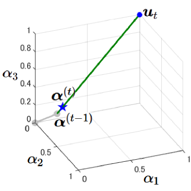
Figure 1: Iteration of Frank-Wolfe algorithm. In $t$-th iteration, the dual problem (9) in which the dual objective $D$ is replaced to its linear approximation (13) is solved. The solution is moved to the point at which the dual objective $D$ is maximized on the line segment between the current solution ${\bm{\alpha}}^{(t-1)}$ and the optimal solution to the sub-problem, say ${\bm{u}}_{t}$.

(a)
(b)	(c)

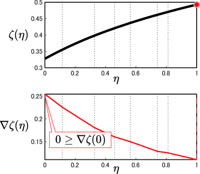
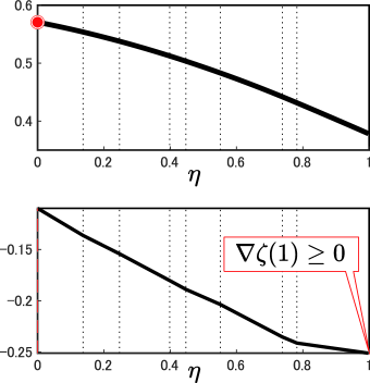
Figure 2: Objective function for line search problem, say $\zeta(\eta)$, is a piecewise quadratic function. In the $h$-th interval $[\theta_{h},\theta_{h+1}]$, the function is expressed in the form of $\zeta(\eta)=a_{h}\eta^{2}+b_{h}\eta+c_{h}$. There are three cases in the line search problem. (a) One of three cases in which $\nabla\zeta(0)>0>\nabla\zeta(1)$. The point $\eta$ with the gradient vanishing is the maximizer of the function $\zeta(\eta)$ in this case. (b) In case of $0\geq\nabla\zeta(0)$, the function $\zeta(\eta)$ attains the maximum at $\eta=1$. (c) In case of $\nabla\zeta(1)\geq 0$, $\zeta(\eta)$ is maximized at $\eta=0$.

5 Dual Problem

The projected gradient algorithm described in the previous section suffers from the lack of a clear criterion for when iterations should be terminated. To obtain a termination criterion, we consider solving a dual problem instead of the primal problem. The following problem is dual to the primal problem (4):

max $$D({\bm{\alpha}})\quad\text{wrt}\quad{\bm{\alpha}}\in[0,1]^{n},$$ (9)

where $$D({\bm{\alpha}}):=-\frac{\lambda}{2}\lVert{\bm{w}}({\bm{\alpha}})\rVert^{2}+\frac{1}{n}\left<{\bm{1}},{\bm{\alpha}}\right>,$$

$${\bm{w}}({\bm{\alpha}}):=\Pi_{{\mathcal{S}}}\left(\frac{1}{\lambda n}{\bm{X}}{\bm{\alpha}}\right).$$

where a $d$-dimensional vector $y_{i}{\bm{x}}_{i}$ is stored in the $i$-th column of the matrix ${\bm{X}}\in{\mathbb{R}}^{d\times n}$. The dual problem for the sign-constrained SVM is reduced to that of the standard SVM when no sign constraints are imposed, which can be seen as follows: in the case of no sign constraints, ${\mathcal{S}}={\mathbb{R}}^{d}$, leading to $\Pi_{{\mathcal{S}}}({\bm{v}})={\bm{v}}$ and ${\bm{w}}({\bm{\alpha}})={\bm{X}}{\bm{\alpha}}/(\lambda n)$; substituting them into (9), the dual problem for the standard SVM is derived. This fact suggests that the difference in the dual objective functions between the sign-constrained and standard SVMs is the presence or absence of the projection onto the feasible region. The projection operation in the dual objective for the sign-constrained SVM precludes the direct use of the standard optimization approach to learning the standard SVM, and thereby makes the optimization problem challenging.

The primal variable optimal to the primal problem (4) can be recovered by ${\bm{w}}_{\star}={\bm{w}}({\bm{\alpha}}_{\star})$ where ${\bm{\alpha}}_{\star}$ is a solution optimal to the dual problem (9), which suggests that iterations in some dual optimization algorithm can be stopped when the duality gap is sufficiently small (i.e. $P({\bm{w}}({\bm{\alpha}}))-D({\bm{\alpha}})\leq\epsilon$). From the nature of the duality:

$$\forall{\bm{\alpha}}\in[0,1]^{n},\qquad P({\bm{w}}({\bm{\alpha}}))\geq P({\bm{w}}_{\star})\geq D({\bm{\alpha}}),$$ (10)

the duality gap lower than a pre-defined threshold $\epsilon$ ensures the primal objective error below the threshold $\epsilon$.

6 Frank-Wolfe Algorithm

In this section, we present a dual optimization algorithm based on the Frank-Wolfe framework [23, 10] for learning the sign constrained SVM. The Frank-Wolfe-based algorithm presented in this section is alternative to the projected gradient algorithm described in the previous section.

In general, the Frank-Wolfe framework performs optimization within a convex polyhedron. The feasible region of the dual problem for the sign-constrained SVM is a hyper-cube which is in a class of convex polyhedrons, suggesting that the dual problem can be a target of the Frank-Wolfe framework.

1 begin

2       Let ${\bm{\alpha}}^{(0)}\in[0,1]^{n}$;

3       for $t:=1$ to $T$ do

4             ${\bm{u}}_{t}\in\mathop{\textrm{argmax}}\limits_{{\bm{u}}\in[0,1]^{n}}\left<\nabla D({\bm{\alpha}}^{(t-1)}),{\bm{u}}\right>$;

5             ${\bm{q}}_{t}:={\bm{u}}_{t}-{\bm{\alpha}}^{(t-1)}$;

6             $\eta_{t}\in\arg\max_{\eta\in[0,1]}D({\bm{\alpha}}^{(t-1)}+\eta{\bm{q}}_{t})$;

7             ${\bm{\alpha}}^{(t)}:={\bm{\alpha}}^{(t-1)}+\eta_{t}{\bm{q}}_{t}$;

8            

9       end for

10      

11 end

12

Algorithm 1 Frank-Wolfe algorithm for solving the dual problem (9).

As described in Algorithm 1, each iteration of the Frank-Wolfe framework consists of two steps, respectively, referred to as the direction finding step and the line search step. In the direction finding step, a linear programming problem is solved. In the sub-problem, the dual objective is replaced with its linear approximation around a previous solution:

$${\bm{u}}\mapsto\left<\nabla D({\bm{\alpha}}^{(t-1)}),{\bm{u}}\right>+D({\bm{\alpha}}^{(t-1)}).$$ (11)

The linear approximation is maximized within the convex polyhedron, yielding a linear programming problem. We denote by ${\bm{u}}_{t}$ the optimal solution to the sub-problem at $t$-th iteration.

In the line search step, the dual objective is maximized on the line segment between the previous solution and the solution optimal to the linear programming problem, say ${\bm{\alpha}}^{(t-1)}$ and ${\bm{u}}_{t}$, respectively. The updated solution can be expressed as ${\bm{\alpha}}^{(t)}:={\bm{\alpha}}^{(t-1)}+\eta_{t}{\bm{q}}_{t}$ where

$$\eta_{t}\in\mathop{\textrm{argmax}}\limits_{\eta\in[0,1]}D({\bm{\alpha}}^{(t-1)}+\eta{\bm{q}}_{t})\text{ and }{\bm{q}}_{t}:={\bm{u}}_{t}-{\bm{\alpha}}^{(t-1)}.$$ (12)

As long as both the sub-problems involved in the two steps are exactly solved at each iteration, the sublinear convergence is ensured. In addition, the accuracy of the solution is guaranteed by use of the duality gap $P({\bm{w}}({\bm{\alpha}}))-D({\bm{\alpha}})$ for a stopping criterion. If the computational cost of each iteration in the Frank-Wolfe algorithm is within $O(nd)$, then the new approach share all the favorable properties of the projected gradient method and simultaneously overcomes the shortcoming. These discussions suggest that both the direction finding step and the line search step need to be computed within $O(nd)$, in order to keep the computational cost of each iteration from exceeding $O(nd)$.

6.1 Direction Finding Step

It is shown here that $O(nd)$ computation accomplishes the direction finding step in the Frank-Wolfe algorithm (Algorithm 1). The direction finding step requires to solve the following sub-problem

min $$\left<\nabla D({\bm{\alpha}}^{(t-1)}),{\bm{u}}\right>\quad\text{wrt}\quad{\bm{u}}\in[0,1]^{n}.$$ (13)

The sub-problem (13) is in a class of linear programming problems. The direction finding step consumes $O(n^{3})$ computation if we resort to a general-purpose linear programming solver. The computational cost $O(n^{3})$ is computationally taxing when training with a large set of training examples.

In this study, we have found a closed-form solution optimal to the linear programming problem (13). The $i$-th entry in the optimal solution ${\bm{u}}_{t}\in[0,1]^{n}$ is expressed as

$$u_{i,t}=\begin{cases}1\qquad\text{if }y_{i}\left<{\bm{w}}({\bm{\alpha}}^{(t-1)}),{\bm{x}}_{i}\right><1,\\ 0\qquad\text{if }y_{i}\left<{\bm{w}}({\bm{\alpha}}^{(t-1)}),{\bm{x}}_{i}\right>\geq 1.\end{cases}$$ (14)

See Subsection 9.1 for the derivation. The optimal solutions to the sub-problem (13) is not unique. The sub-linear convergence is ensured even if taking any point among the set of the optimal solutions.

Time Complexity of Direction Finding Step: The procedure and the time complexities for computation of the closed-form solution (14) are summarized as follows.

Compute ${\bm{v}}^{(t-1)}:={\bm{X}}{\bm{\alpha}}^{(t-1)}/(\lambda n)$;	$O(nd)$.
Compute ${\bm{w}}^{(t-1)}:=\Pi_{{\mathcal{S}}}({\bm{v}}^{(t-1)})$;	$O(d)$.
Compute ${\bm{z}}^{(t-1)}:={\bm{X}}^{\top}{\bm{w}}^{(t-1)}$;	$O(nd)$.
$\forall i\in[n]$, $u_{i,t}:=\mathds{1}(1\leq z_{i}^{(t-1)})$;	$O(n)$.

Therein, $z_{i}^{(t-1)}$ is the $i$-th entry in the vector ${\bm{z}}^{(t-1)}$, and the function $\mathds{1}(\cdot)$ takes the value of one if the logical argument is true; otherwise zero. The line search problem can, thus, be solved in $O(nd)$ when $d$ is within $O(n)$.

6.2 Line Search Step

It has been seen that the direction finding step can be performed within $O(nd)$ computational cost. It shall be shown here that the line search step requires only $O(nd)$ cost, too. Line search is an operation that finds an optimal solution, denoted by $\eta_{\star}\in[0,1]$, to the sub-problem:

max $$\zeta(\eta)\quad\text{wrt}\quad\eta\in[0,1],$$ (15)

where $$\zeta(\eta):=D({\bm{\alpha}}+\eta{\bm{q}}),\quad{\bm{\alpha}}\in[0,1]^{n},$$

$${\bm{q}}\in[0,1]^{n}-{\bm{\alpha}},\,\,{\bm{q}}\neq{\bm{0}}_{n}.$$

In case of ${\bm{q}}={\bm{0}}_{n}$, it is obvious that any $\eta\in[0,1]$ is optimal. Here, our discussion is limited to the case ${\bm{q}}\neq{\bm{0}}_{n}$ as given in (15). The following is the key lemma for solving the line search problem.

Lemma 1.

The objective function of the sub-problem given in (15), say $\zeta:[0,1]\to{\mathbb{R}}$, is a differentiable and concave piecewise quadratic function and its derivative is continuous and monotonically decreasing. Namely, there exist an integer $d_{t}\in[d+1]$, coefficients $(a_{k},b_{k},c_{k})$ for $k\in[d_{t}]$ with $a_{k}\leq 0$ and $\theta_{0},\dots,\theta_{d_{t}+1}$ such that $0=\theta_{1}<\theta_{2}<\dots<\theta_{d_{t}+1}=1$ and the function can be expressed as $\forall k\in[d_{t}]$, $\forall\eta\in[\theta_{k},\theta_{k+1}]$,

$$\zeta(\eta)=a_{k}\eta^{2}+b_{k}\eta+c_{k},$$ (16)

and $\forall k\in[d_{t}-1]$,

$$2a_{k}\theta_{k+1}+b_{k}=2a_{k+1}\theta_{k+1}+b_{k+1}.$$ (17)

See Subsection 9.2 for the proof of Lemma 1.

Solution to Line Search: Lemma 1 suggests that three cases described in Figure 2. From this observation, it turns out that an optimal solution to the line search problem (15) can be given in a closed-form as

$$\eta_{\star}=\begin{cases}0\qquad&\text{if }b_{1}\leq 0,\\ 1\qquad&\text{if }2a_{d_{t}+1}+b_{d_{t}+1}\geq 0,\\ -\frac{b_{k_{\star}}}{2a_{k_{\star}}}\qquad&\text{if $b_{1}>0$, $2a_{d_{t}+1}+b_{d_{t}+1}<0$, $a_{k_{\star}}<0$,}\\ \theta_{k_{\star}}\qquad&\text{if $b_{1}>0$, $2a_{d_{t}+1}+b_{d_{t}+1}<0$, $a_{k_{\star}}=0$}\end{cases}$$ (18)

where $k_{\star}\in[d_{t}]$ here is the index of one of $d_{t}$ intervals, in which the derivative vanishes at some point. Namely,

$$2a_{k_{\star}}\theta_{k_{\star}}+b_{k_{\star}}\geq 0\quad\text{ and }\quad 2a_{k_{\star}}\theta_{k_{\star}+1}+b_{k_{\star}}\leq 0.$$ (19)

Note that, from the definition of $k_{\star}$, it must hold that $b_{k_{\star}}=0$ in the case that $b_{1}>0$, $2a_{d_{t}+1}+b_{d_{t}+1}<0$ and $a_{k_{\star}}=0$.

Endpoints and Coefficients of Piecewise Quadratic Function $\zeta$: Here we describe how to determine the endpoints $\theta_{1},\theta_{2},\dots,\theta_{d_{t}+1}\in[0,1]$ and the coefficients of the piecewise quadratic function $\zeta$, say $(a_{k},b_{k},c_{k})$ for $k=1,\dots,d_{t}$.

Let ${\bm{v}}_{0}:=\left[v_{1,0},\dots,v_{d,0}\right]^{\top}$ and ${\bm{v}}_{q}:=\left[v_{1,q},\dots,v_{d,q}\right]^{\top}$ have the following entries, $\forall h\in[d]$,

$$v_{h,0}:=\frac{1}{\lambda n}\left<{\bm{f}}_{h},{\bm{\alpha}}\right>,\quad v_{h,q}:=\frac{1}{\lambda n}\left<{\bm{f}}_{h},{\bm{u}}-{\bm{\alpha}}\right>.$$ (20)

where ${\bm{f}}_{h}\in{\mathbb{R}}^{n}$ is the $h$-th column vector in ${\bm{X}}^{\top}$. Let

$$\Theta:=\Bigg{\{}\theta\in[0,1]\,\Bigg{|}\,\exists h\in{\mathcal{I}}_{+}\\ \text{ s.t. }v_{h,q}\neq 0,\,\theta=-\frac{v_{h,0}}{v_{h,q}}\Bigg{\}}\cup\{0,1\}.$$ (21)

The number of intervals $d_{t}$ can be set to the cardinality of the set $\Theta$ minus one (i.e. $d_{t}=\text{card}(\Theta)-1$) and the endpoints $\theta_{1},\dots,\theta_{d_{t}+1}$ of $d_{t}$ intervals are determined by sorting the elements in $\Theta$ so that $\theta_{1}<\theta_{2}<\dots<\theta_{d_{t}+1}$. In this setting, it can be observed that equation (16) is satisifed if coefficients are given as $\forall k\in[d_{t}]$,

$$a_{k}:=-\frac{\lambda}{2}\sum_{h\in{\mathcal{H}}_{k}}v_{h,q}^{2},$$ (22)

$$b_{k}:=\frac{1}{n}\left<{\bm{1}},{\bm{u}}-{\bm{\alpha}}\right>-\lambda\sum_{h\in{\mathcal{H}}_{k}}v_{h,q}v_{h,0},$$

$$c_{k}:=\frac{1}{n}\left<{\bm{1}},{\bm{\alpha}}\right>-\frac{\lambda}{2}\sum_{h\in{\mathcal{H}}_{k}}v_{h,0}^{2}$$

where

$${\mathcal{H}}_{k}:={\mathcal{I}}_{0}\cup\left\{h\in{\mathcal{I}}_{+}\,\middle|\,v_{h,0}+\frac{\theta_{k}+\theta_{k+1}}{2}v_{h,q}>0\right\}.$$ (23)

Time Complexity of Line Search Step: The procedure required to compute the solution (18) and the time complexity of each step is described as follows.

Compute ${\bm{v}}_{0}$ and ${\bm{v}}_{q}$;	$O(nd)$.
Determine $\Theta$;	$O(d)$.
Sort the elements in $\Theta$;	$O(d\log d)$.
Compute ${\mathcal{H}}_{k}$ for $k\in[d_{t}]$;	$O(d^{2})$.
Compute coefficients $(a_{k},b_{k},c_{k})$ for $k\in[d_{t}]$;	$O(d^{2})$.
Find $k_{\star}$;	$O(d)$.
Compute a solution (18);	$O(1)$.

Hence the line search problem can be solved in $O(nd)$ when $d$ is within $O(n)$.

6.3 Convergence Analysis

We have seen that the direction finding step and the line search step can be performed exactly, meaning that our algorithm inherits the theoretical guarantee for the convergence property of the Frank-Wolfe algorithm. In general, the objective error of the Frank-Wolfe algorithm for a minimization problem is bounded as

$$F({\bm{x}}^{(T)})-F({\bm{x}}_{\star})\leq\frac{2C_{F}}{T+2}$$ (24)

where $C_{F}$ is the curvature of the continuously differentiable and convex objective function $F$ to be minimized [10]. The curvature [10] is defined as

$$C_{F}:=\sup\Big{\{}\frac{2}{\gamma^{2}}{\mathcal{D}}_{F}({\bm{y}}_{\gamma}\,;\,{\bm{x}})\,\Big{|} \,{\bm{u}},{\bm{x}}\in{\mathcal{M}},\,\gamma\in(0,1],\,$$ (25)

$${\bm{y}}_{\gamma}:=(1-\gamma){\bm{x}}+\gamma{\bm{u}}\Big{\}},$$

where ${\mathcal{M}}$ is the domain of the minimization problem and ${\mathcal{D}}_{F}({\bm{y}}\,;\,{\bm{x}})$ is the Bregman divergence. We obtained the following bound for the curvature of the objective in the dual problem (9).

Lemma 2.

Assume that the norm of every feature vector is $R$, at most (i.e. $\forall i\in[n]$, $\lVert{\bm{x}}_{i}\rVert\leq R$). The curvature for $F:=-D$ with ${\mathcal{M}}:=[0,1]^{n}$ is then bounded as $C_{F}\leq R^{2}/\lambda$.

See Subsection 9.3 for the proof of Lemma 2.

This lemma leads to our main result:

Theorem 6.1.

Suppose that $\forall i\in[n]$, $\lVert{\bm{x}}_{i}\rVert\leq R$. Each iteration of Algorithm 1 can be performed within $O(nd)$ computational cost. The objective error is less than or equal to a positive scalar $\epsilon>0$ (i.e. $D({\bm{\alpha}}_{\star})-D({\bm{\alpha}}^{(T)})\leq\epsilon$) for any $T\in{\mathbb{N}}$ such that

$$T\geq\frac{2R^{2}}{\lambda\epsilon}-2.$$ (26)

Table 1: ROC scores for amino acid sequence classification.

Class	Conventional SVM-pairwise	Sign Constrained SVM-pairwise
1	0.731 (0.009)	0.749 (0.010)
2	0.681 (0.013)	0.756 (0.012)
3	0.735 (0.013)	0.758 (0.012)
4	0.745 (0.010)	0.768 (0.009)
5	0.709 (0.017)	0.784 (0.008)
6	0.625 (0.007)	0.692 (0.012)
7	0.628 (0.023)	0.702 (0.030)
8	0.664 (0.018)	0.733 (0.018)
9	0.603 (0.019)	0.681 (0.022)
10	0.712 (0.008)	0.739 (0.010)
11	0.523 (0.026)	0.561 (0.029)
12	0.894 (0.013)	0.905 (0.012)

7 Experiments

In this section, we illustrate how fast the optimization algorithm converge in real-world data, and empirically show how well the sign constraints work for the task of biological sequence classification.

7.1 Convergence

We examine the convergence of the projected gradient and the Frank-Wolfe algorithms on the Cora and MNIST datasets. Cora dataset is a collection of 15,396 academic papers related to computer science [33]. Each paper is annotated manually to provide a hierarchical classification. The dataset has ten categories at the top hierarchy. We divided the top categories into two groups to pose a binary classification problem. The positive class consists of IR, AI, OS, HA, and Pr, and the negative class is from Da, EC, Ne, DA, and HCI, resulting 10,778 and 4,618 papers belong to the positive and negative class, respectively. The task here is to classify each paper from the normalized word frequencies in its title. After removing stop words, 12,644 words used in the title of 15,396 papers were found. Each 12,644-dimensional feature vector is normalized with Euclidean norm. The MNIST dataset is the most popular dataset for benchmarking machine learning methodologies. The dataset has 60,000 handwritten digit images. Each image has 784 pixels. For this simulation, images of odd digits (i.e. ‘1’, ‘3’, ‘5’, ‘7’, ‘9’) and even digits (i.e. ‘0’, ‘2’, ‘4’, ‘6’, ‘8’) were labeled as positive and negative, respectively. Each feature vector is normalized to transform each of examples to a unit vector.

A hundred iterations of the projected gradient and the Frank-Wolfe algorithms were run and the primal objective values $P({\bm{w}})$ were monitored 55 times at different iterations. The iteration numbers at which the objective function was evaluated were spaced evenly on a logarithmic scale (i.e. $t=1,2,3,\dots,50,53,55,\dots,87,92,96,100$). The minima among these objective errors monitored so far were recorded. For the Frank-Wolfe Algorithm, the duality gaps $P({\bm{w}})-D({\bm{\alpha}})$ were also evaluated. The regularization parameter $\lambda$ was varied with $\lambda=10^{-6}/n,10^{-4}/n,10^{-2}/n$ where $n=15,396$ for Cora and $n=60,000$ for MNIST. In order to examine how fast each algorithm converges, the true objective error should be assesed, although it is impossible because $P({\bm{w}}_{\star})$ is usually unknown. To approximate the objective error, we ran the Frank-Wolfe algorithm to compute the dual objective value at $T^{\prime}:=1,000$th iteration. Although $D({\bm{\alpha}}^{(T^{\prime})})$ might be slightly smaller than the true minimal primal objective value $\min_{{\bm{w}}\in{\mathcal{S}}}P({\bm{w}})$, the value $P({\bm{w}})-D({\bm{\alpha}}^{(T^{\prime})})$ was regarded as the objective error.

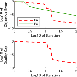
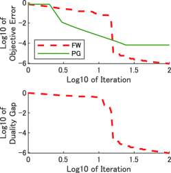
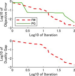
Figure 3: Convergence on Cora. FW and PG are the abbreviations of Frank-Wolfe and projected gradient, respectively.

The upper row in Figure 3 plots the objective errors against iteration numbers on Cora, respectively. For all $\lambda$ on Cora, the projected gradient algorithm achieved smaller objective errors at around ten iterations, whereas the objective errors of the Frank-Wolfe were much smaller than those of the projected gradient after 15 iterations. For MNIST (See Figure 4), the Frank-Wolfe converged to the minimum much faster than the projected gradient. The lower row depicts the duality gaps produced from the Frank-Wolfe. Recall that the duality gap can be a clear stopping criterion ensuring the quality of the solution. The duality gaps were indeed converged to zero, implying that the duality gap can be utilized as a stopping criterion.

7.2 Biological Sequence Classification

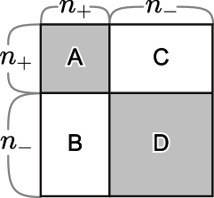
Figure 5: Training data and sign constraints for SVM-pairwise. In SVM-pairwise approach, features are sequence similarities to training data. Feature vectors for training SVM are columns of a square similarity matrix among training data. For simplicity, we assume that amino acid sequences are re-ordered so that first $n_{+}$ positive sequences are followed by $n_{-}$ negative sequences. In this assumption, the sub-matrix A of the similarity matrix is among positive examples, D is among negatives, B and C are of positives against negatives. Weight coefficients for sub-matrices A and C correspond to non-negative sign constraints ${\mathcal{I}}_{+}$, whereas weight coefficients for B and D correspond to non-positive sign constraints ${\mathcal{I}}_{-}$.

Here we demonstrate that sign constraints are a powerful methodology for boosting the prediction performance for SVM-pairwise [24] which is a binary classifier of biological sequences. SVM-pairwise predicts the existence/absence of a property of a query protein from its amino-acid sequence. Conventional analysis of biological sequences is based on pairwise comparison between two sequences using a sequence similarity measure such as the Smith Waterman score [35]. SVM-pairwise was developed to predict the remote homology by combining the sequence comparison with supervised machine learning. The feature vector taken by SVM-pairwise is the sequence similarities to each of sequences for training. If $n$ proteins are in a training dataset, the feature vector has $n$ entries, $x_{1},\dots,x_{n}$. If we assume that the first $n_{+}$ proteins in the training set are annotated as positive and the rest of $n_{-}:=n-n_{+}$ proteins negative, then the first $n_{+}$ entries $x_{1},\dots,x_{n_{+}}$ are the sequence similarities to positive proteins and $x_{n_{+}+1},\dots,x_{n}$ are the similarities to negative proteins. Since each feature vector for training is $n$-dimensional, the data matrix ${\bm{X}}$ is square (See Figure 5). The prediction score for a query protein ${\bm{x}}$ is the difference from

$$w_{1}x_{1}+\dots+w_{n_{+}}x_{n_{+}}$$ (27)

to

$$-w_{n_{+}+1}x_{n_{+}+1}-\dots-w_{n}x_{n}.$$ (28)

From this view, it is preferable that the first $n_{+}$ weight coefficients $w_{1},\dots,w_{n_{+}}$ are non-negative and that the remaining $n_{-}$ coefficients $w_{n_{+}+1},\dots,w_{n}$ are non-positive. Nevertheless, the pairwise SVM does not ensure these requirements. These observations motivated us to impose these constraints explicitly as $w_{1}\geq 0,\dots,w_{n_{+}}\geq 0$ and $w_{n_{+}+1}\leq 0,\dots,w_{n}\leq 0$.

We examined the effectiveness of sign constraints on 3,583 yeast proteins with the annotations for these cellular functions and the Smith-Waterman similarities available from https://noble.gs.washington.edu/proj/sdp-svm/. The annotation of cellular function of a protein was existence or absence for each of 12 functional categories. We posed 12 independent binary classification task. A half of 3,583 proteins were selected randomly and used for training and the rest were used for testing. We performed five-fold cross-validation within a training subset to determine the value of the regularization constant. Weight coefficients ${\bm{w}}\in{\mathbb{R}}^{n}$ were determined by conventional SVM-pairwise and sign-constrained SVM-pairwise, respectively. For each of 12 binary classification tasks, ten ROC scores for conventional SVM-pairwise and ten ROC scores for sign-constrained SVM-pairwise were obtained by repeating this procedure ten times. The one-sample t-test was performed to detect the significant difference between two ROC scores. The average of ROC scores and the standard deviations over ten repetitions were shown in Table 1. The best ROC scores are bold-faced and the underlined scores do not have a statistical significant difference from the best performance. Additional results are given in Subsection 10.2. For all of 12 tasks, sign constrained modification consistently improved the ROC scores, suggesting that the sign constraints are a promising technique for SVM-pairwise framework.

8 Conclusion

In this paper, we discussed the projected gradient algorithm and the Frank-Wolfe algorithm for learning the linear SVM under sign constraints. We provided solid analyses for the computational cost of each iteration and the convergence rate both for the two optimization algorithms. We found that both algorithms were ensured to have the sublinear convergence rate and the $O(nd)$ computational cost for each iteration. Finally, we proposed to introduce sign constraints for the SVM-pairwise approach and empirically demonstrated the promising prediction performances on 12 binary classification tasks for cellular functional prediction. SVM-pairwise is an approach specialized for computational biology, although similar approaches have also been discussed in more general settings [36, 28]. Benchmarking the effects of sign constraints on SVM-pairwise in other applications will be the subject of future work.

9 Derivations and Proofs

9.1 Derivation for (14)

Observe that the linear programming problem of an $n$-dimensional variable ${\bm{u}}$ given in (13) can be decomposed into $n$ independent problems: $\forall i\in[n]$,

$$\max g_{i}^{(t-1)}u_{i}\quad\text{wrt}\quad u_{i}\in[0,1],$$ (29)

where $$g_{i}^{(t-1)}:=\left.\frac{\partial D({\bm{\alpha}})}{\partial\alpha_{i}}\right|_{{\bm{\alpha}}={\bm{\alpha}}^{(t-1)}}.$$

It can be seen that the gradient $g_{i}^{(t-1)}$ is expressed as

$$g_{i}^{(t-1)}=\frac{1}{n}\left(1-\left<{\bm{w}}({\bm{\alpha}}^{(t-1)}),{\bm{x}}_{i}\right>\right)$$ (30)

From this, we get

$$\mathds{1}\left[\left<{\bm{w}}({\bm{\alpha}}^{(t-1)}),{\bm{x}}_{i}\right><1\right]=\\ \mathds{1}\left[g_{i}^{(t-1)}>0\right]\in\text{argmax}_{u_{i}\in[0,1]}g_{i}^{(t-1)}u_{i}$$ (31)

which implies that the vector with $i$-th entry $\mathds{1}\left[\left<{\bm{w}}({\bm{\alpha}}^{(t-1)}),{\bm{x}}_{i}\right><1\right]$, as defined in (14), is a solution optimal to the linear programming problem (13). ∎

9.2 Proof for Lemma 1

The fact that $\forall k\in[d_{t}]$, $a_{k}\leq 0$ is apparent when coefficients and endpoints are determined as in (LABEL:eq:coef-piesequadfun) and the descriptions around the equation. Let $w_{h}({\bm{\alpha}})$ and $v_{h}({\bm{\alpha}})$ be the $h$-th entries in two vectors ${\bm{w}}({\bm{\alpha}})$ and ${\bm{v}}({\bm{\alpha}})$, respectively. Let ${\bm{q}}:={\bm{u}}-{\bm{\alpha}}$. We first use the following lemma to show that the setting of coefficients and endpoints defined in Subsection 6.2 actually establishes (16).

Lemma 3.

Let an arbitrary $\eta\in[0,1]$ and let $k\in[d_{t}]$ such that $\eta\in[\theta_{k},\theta_{k+1}]$. It then holds that

$$w_{h}({\bm{\alpha}}+\eta{\bm{q}})=\begin{cases}v_{h,0}+\eta v_{h,q}&\qquad\text{if }h\in{\mathcal{H}}_{k},\\ 0&\qquad\text{if }h\in[d]\setminus{\mathcal{H}}_{k},\end{cases}$$ (32)

Proof for Lemma 3 The equality (32) holds apparently for $h\in{\mathcal{H}}_{k}\setminus{\mathcal{I}}_{+}$. We observe that

$$\forall\eta\in(\theta_{k},\theta_{k+1}),\quad v_{h,0}+\eta v_{h,q}\neq 0.$$ (33)

For $h\in[d]\setminus{\mathcal{H}}_{k}={\mathcal{I}}_{+}\setminus{\mathcal{H}}_{k}$, the continuity of the linear function $\eta\mapsto v_{h,q}+\eta v_{h,q}$ implies that

$$\forall\eta\in(\theta_{k},\theta_{k+1}),\quad 0>v_{h,0}+\eta v_{h,q}$$ (34)

implying $w_{h}({\bm{\alpha}}+\eta{\bm{q}})=0$. For $h\in{\mathcal{I}}_{+}\cap{\mathcal{H}}_{k}$, the continuity of the linear function $\eta\mapsto v_{h,q}+\eta v_{h,q}$ implies

$$\forall\eta\in(\theta_{k},\theta_{k+1}),\quad 0<v_{h,0}+\eta v_{h,q}=w_{h}({\bm{\alpha}}+\eta{\bm{q}}).$$ (35)

End of proof for Lemma 3

With help of Lemma 3, the square of the norm of the vector ${\bm{w}}({\bm{\alpha}}+\eta{\bm{q}})$ is expressed as

$$\frac{1}{2}\lVert{\bm{w}}({\bm{\alpha}}+\eta{\bm{q}})\rVert^{2}=\frac{1}{2}\sum_{h\in[d]}(w_{h}({\bm{\alpha}}+\eta{\bm{q}}))^{2}\\ =\frac{1}{2}\sum_{h\in{\mathcal{H}}_{k}}v_{h,q}^{2}\eta^{2}+2\eta v_{h,0}v_{h,q}+v_{h,0}^{2}$$ (36)

which derives the equality of (16) as

$$\zeta(\eta) =D({\bm{\alpha}}+\eta{\bm{q}})$$ (37)

$$=-\frac{\lambda}{2}\lVert{\bm{w}}({\bm{\alpha}}+\eta{\bm{q}})\rVert^{2}+\frac{1}{n}\left<{\bm{1}},{\bm{\alpha}}+\eta{\bm{q}}\right>$$

$$=-\frac{\lambda}{2}\sum_{h\in{\mathcal{H}}_{k}}v_{h,q}^{2}\eta^{2}+\left(\frac{1}{n}\left<{\bm{1}},{\bm{q}}\right>-\lambda\sum_{h\in{\mathcal{H}}_{k}}v_{h,0}v_{h,q}\right)\eta$$

$$\qquad+\frac{1}{n}\left<{\bm{1}},{\bm{\alpha}}\right>-\frac{\lambda}{2}\sum_{h\in{\mathcal{H}}_{k}}v_{h,0}^{2}$$

$$=a_{k}\eta^{2}+b_{k}\eta+c_{k}.$$

We next show the equality of (17). We partition the index set ${\mathcal{H}}_{k}$ into three exclusive subsets ${\mathcal{H}}_{1,k}$, ${\mathcal{H}}_{2,k}$, ${\mathcal{H}}_{3,k}$, each of which is defined as

$${\mathcal{H}}_{1,k}:={\mathcal{H}}_{k}\cap{\mathcal{H}}_{k+1}, {\mathcal{H}}_{2,k}:={\mathcal{H}}_{k}\setminus{\mathcal{H}}_{k+1},$$ (38)

$${\mathcal{H}}_{3,k}:={\mathcal{H}}_{k+1}\setminus{\mathcal{H}}_{k},$$

respectively. Observe that

$$\forall h\in{\mathcal{H}}_{2,k}\cup{\mathcal{H}}_{3,k},\qquad v_{h,0}+\theta_{k+1}v_{h,q}=0,$$ (39)

which follows from the combination of two properties: the continuity of the linear function $\eta\mapsto v_{h,q}+\eta v_{h,q}$ and the change of the sign at $\eta=\theta_{k+1}$, i.e.,

$$\forall h\in{\mathcal{H}}_{2,k}, \forall\eta_{1}\in(\theta_{k},\theta_{k+1}),\quad v_{h,0}+\eta_{1}v_{h,q}>0,\text{ and }$$ (40)

$$\forall\eta_{2}\in(\theta_{k+1},\theta_{k+2}),\quad v_{h,0}+\eta_{2}v_{h,q}\leq 0,$$

and

$$\forall h\in{\mathcal{H}}_{3,k}, \forall\eta_{1}\in(\theta_{k},\theta_{k+1}),\quad v_{h,0}+\eta_{1}v_{h,q}\leq 0,\text{ and }$$ (41)

$$\forall\eta_{2}\in(\theta_{k+1},\theta_{k+2}),\quad v_{h,0}+\eta_{2}v_{h,q}>0.$$

From (39), the difference of RHS from LHS in (17) can be written as

$$2a_{k+1}\theta_{k+1}+b_{k+1}-(2a_{k}\theta_{k+1}+b_{k})$$ (42)

$$=\sum_{h\in{\mathcal{H}}_{2,k}}\left(v_{h,q}^{2}\theta_{k+1}+v_{h,q}v_{h,0}\right)$$

$$\qquad-\sum_{h\in{\mathcal{H}}_{3,k}}\left(v_{h,q}^{2}\theta_{k+1}+v_{h,q}v_{h,0}\right)$$

$$=\sum_{h\in{\mathcal{H}}_{2,k}}\left(v_{h,q}\theta_{k+1}+v_{h,0}\right)v_{h,q}$$

$$\qquad-\sum_{h\in{\mathcal{H}}_{3,k}}\left(v_{h,q}\theta_{k+1}+v_{h,0}\right)v_{h,q}$$

$$=\sum_{h\in{\mathcal{H}}_{2,k}}0-\sum_{h\in{\mathcal{H}}_{3,k}}0=0.$$

∎

9.3 Proof for Lemma 2

Let ${\bm{f}}_{h}$ be the $h$th column of ${\bm{X}}^{\top}$. We then have

$$v_{h}({\bm{\alpha}}) =\frac{1}{\lambda n}\left<{\bm{f}}_{h},{\bm{\alpha}}\right>\qquad\text{and}$$ (43)

$$w_{h}({\bm{\alpha}}) =\begin{cases}v_{h}({\bm{\alpha}})&\quad\text{ if }\sigma_{h}=0,\\ \max(0,v_{h}({\bm{\alpha}}))&\quad\text{ if }\sigma_{h}=1.\end{cases}$$

Let

$${\mathcal{H}}_{{\bm{\alpha}}}:=\left\{h\in[d]\,\middle|\,\sigma_{h}=0\text{ or }v_{h}({\bm{\alpha}})>0\right\}$$ (44)

and

$${\bm{K}}_{{\bm{\alpha}}}:=\sum_{h\in{\mathcal{H}}_{{\bm{\alpha}}}}{\bm{f}}_{h}{\bm{f}}_{h}^{\top}.$$ (45)

For the negative second-order derivative of the objective, we have

$$-\nabla^{2}D({\bm{\alpha}})=\frac{1}{\lambda n^{2}}{\bm{K}}_{{\bm{\alpha}}}=\frac{1}{\lambda n^{2}}\sum_{h\in{\mathcal{H}}_{{\bm{\alpha}}}}{\bm{f}}_{h}{\bm{f}}_{h}^{\top}\\ \preceq\frac{1}{\lambda n^{2}}\sum_{h=1}^{d}{\bm{f}}_{h}{\bm{f}}_{h}^{\top}=\frac{1}{\lambda n^{2}}{\bm{X}}^{\top}{\bm{X}}.$$ (46)

Therein, we have used the notation $\preceq$ to denote the generalized inequality associated with the positive semidefinite cone (i.e. for two symmetric matrices, ${\bm{A}}$ and ${\bm{B}}$, we can write ${\bm{A}}\preceq{\bm{B}}$ if ${\bm{B}}-{\bm{A}}$ is positive semidefinite. ).

The term of Bregman divergence in the definition of the curvature (25) is bounded as $\forall{\bm{u}},\forall{\bm{\alpha}}\in{\mathcal{M}}$, $\forall\gamma\in[0,1]$, $\exists\eta\in[0,\gamma]$,

$${\mathcal{D}}_{-D}({\bm{y}}_{\gamma}\,;\,{\bm{\alpha}}) =D({\bm{\alpha}})-D({\bm{y}}_{\gamma})+\left<\nabla D({\bm{\alpha}}),{\bm{y}}_{\gamma}-{\bm{\alpha}})\right>$$ (47)

$$=-\frac{1}{2}\left<{\bm{y}}_{\gamma}-{\bm{\alpha}},\nabla^{2}D({\bm{y}}_{\eta})({\bm{y}}_{\gamma}-{\bm{\alpha}})\right>$$

$$=-\frac{\gamma^{2}}{2}\left<{\bm{u}}-{\bm{\alpha}},\nabla^{2}D({\bm{y}}_{\eta})({\bm{u}}-{\bm{\alpha}})\right>$$

$$\leq\frac{\gamma^{2}}{2\lambda n^{2}}\left<{\bm{u}}-{\bm{\alpha}},{\bm{X}}^{\top}{\bm{X}}({\bm{u}}-{\bm{\alpha}})\right>$$

$$=\frac{\gamma^{2}}{2\lambda n^{2}}\lVert{\bm{X}}({\bm{u}}-{\bm{\alpha}})\rVert^{2}$$

where we have used Taylor’s theorem to obtain the equality in the second line, and the inequality in the fourth line follows from (46). Therefore, we have

$$C_{F} =\sup\Bigg{\{}\frac{2}{\gamma^{2}}{\mathcal{D}}_{-D}({\bm{y}}_{\gamma}\,;\,{\bm{\alpha}})\,\Bigg{|}\,$$ (48)

$$\qquad\qquad{\bm{u}},{\bm{\alpha}}\in[0,1]^{n},\,\gamma\in(0,1],\eta\in[0,\gamma]\Bigg{\}}$$

$$\leq\sup\left\{\frac{1}{\lambda n^{2}}\lVert{\bm{X}}({\bm{u}}-{\bm{\alpha}})\rVert^{2}\,\middle|\,{\bm{u}},{\bm{\alpha}}\in[0,1]^{n}\right\}$$

$$=\sup\left\{\frac{1}{\lambda n^{2}}\lVert{\bm{X}}{\bm{\beta}}\rVert^{2}\,\middle|\,{\bm{\beta}}\in[-1,+1]^{n}\right\}$$

We now use the fact that $\forall{\bm{\beta}}\in[-1,+1]^{n}$,

$$\lVert{\bm{X}}{\bm{\beta}}\rVert=\lVert\sum_{i=1}^{n}\beta_{i}{\bm{x}}_{i}\rVert\leq\sum_{i=1}^{n}\lVert\beta_{i}{\bm{x}}_{i}\rVert\leq\sum_{i=1}^{n}\lVert{\bm{x}}_{i}\rVert\leq nR,$$ (49)

to get

$$C_{F} \leq\frac{1}{\lambda n^{2}}(nR)^{2}=\frac{R^{2}}{\lambda}.$$ (50)

∎

10 Details on Experimental Results

10.1 Additional Experimental Results for Convergence

The convergence behaviors on MNIST are demonstrated in Figure 4. The experimental settings are described in the main text.

(a) $\lambda=10^{-6}/n$	(b) $\lambda=10^{-4}/n$	(c) $\lambda=10^{-2}/n$

(a) $\lambda=10^{-6}/n$	(b) $\lambda=10^{-4}/n$	(c) $\lambda=10^{-2}/n$

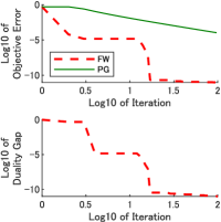
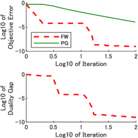
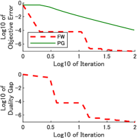
Figure 4: Convergence on MNIST.

10.2 Additional Experimental Results for Amino Acid Sequence Classification

Table 2: Details on ROC scores for amino acid sequence classification.

	Conventional SVM-pairwise
	$\lambda=10^{-6}/n$	$\lambda=10^{-4}/n$	$\lambda=10^{-2}/n$	$\lambda=10^{0}/n$	$\lambda=10^{2}/n$
1	0.734 (0.010)	0.734 (0.010)	0.734 (0.010)	0.732 (0.010)	0.626 (0.011)
2	0.681 (0.022)	0.681 (0.022)	0.681 (0.022)	0.675 (0.020)	0.544 (0.023)
3	0.718 (0.011)	0.718 (0.011)	0.718 (0.011)	0.715 (0.010)	0.548 (0.014)
4	0.743 (0.009)	0.743 (0.009)	0.743 (0.009)	0.739 (0.008)	0.525 (0.009)
5	0.718 (0.011)	0.718 (0.011)	0.718 (0.011)	0.697 (0.010)	0.468 (0.021)
6	0.639 (0.012)	0.639 (0.012)	0.639 (0.012)	0.625 (0.012)	0.519 (0.011)
7	0.626 (0.029)	0.626 (0.029)	0.626 (0.029)	0.613 (0.026)	0.571 (0.015)
8	0.667 (0.022)	0.667 (0.022)	0.667 (0.022)	0.665 (0.022)	0.633 (0.028)
9	0.585 (0.024)	0.585 (0.024)	0.585 (0.024)	0.579 (0.020)	0.492 (0.024)
10	0.712 (0.013)	0.712 (0.013)	0.712 (0.013)	0.708 (0.012)	0.578 (0.011)
11	0.526 (0.025)	0.526 (0.025)	0.526 (0.025)	0.495 (0.024)	0.462 (0.016)
12	0.901 (0.013)	0.901 (0.013)	0.901 (0.013)	0.899 (0.013)	0.764 (0.015)
	Sign Constrained SVM-pairwise
	$\lambda=10^{-6}/n$	$\lambda=10^{-4}/n$	$\lambda=10^{-2}/n$	$\lambda=10^{0}/n$	$\lambda=10^{2}/n$
1	0.752 (0.011)	0.752 (0.011)	0.752 (0.011)	0.754 (0.012)	0.755 (0.011)
2	0.749 (0.020)	0.749 (0.020)	0.749 (0.020)	0.731 (0.020)	0.676 (0.018)
3	0.744 (0.009)	0.744 (0.009)	0.744 (0.009)	0.745 (0.008)	0.646 (0.010)
4	0.769 (0.009)	0.769 (0.009)	0.769 (0.009)	0.766 (0.009)	0.684 (0.010)
5	0.781 (0.015)	0.781 (0.015)	0.781 (0.015)	0.768 (0.014)	0.680 (0.010)
6	0.699 (0.009)	0.699 (0.009)	0.699 (0.009)	0.697 (0.011)	0.634 (0.008)
7	0.710 (0.021)	0.710 (0.021)	0.710 (0.021)	0.713 (0.020)	0.695 (0.010)
8	0.728 (0.015)	0.728 (0.015)	0.728 (0.015)	0.722 (0.019)	0.689 (0.025)
9	0.670 (0.027)	0.670 (0.027)	0.670 (0.027)	0.653 (0.027)	0.608 (0.025)
10	0.741 (0.016)	0.741 (0.016)	0.741 (0.016)	0.743 (0.017)	0.645 (0.014)
11	0.564 (0.018)	0.564 (0.018)	0.564 (0.018)	0.533 (0.020)	0.487 (0.018)
12	0.909 (0.012)	0.909 (0.012)	0.909 (0.012)	0.908 (0.012)	0.857 (0.013)

Here we report more details of the experimental results on amino acid sequence classification. As described in Subsection 7.2, the procedure for dividing a set of 3,583 proteins into training and testing subsets was repeated 10 times to obtain ten divisions. For each division and each of 12 classification tasks, SVM was trained with the SVM-pairwise framework under sign constraints. Regularization parameter $\lambda$ was varied with $\lambda=10^{-6}/n,10^{-4}/n,10^{-2}/n,10^{0}/n,10^{2}/n$. The lower table in Table 2 shows the average ROC scores and the standard deviations over ten repetitions. Similar procedure with the conventional SVM-pairwise was performed to obtain the upper table. The bold-faced figures in the table represent the best performance for the binary classification task. The underlined figures indicate that the performance is not significantly different from the best performance. The prediction performances in Table 1 are the best ROC scores of the sign-constrained SVM-pairwise and the best ones of the conventional SVM-pairwise. In this application, weaker regularization tends to get a better prediction performance both for the two methods.

References

- [1] S. F. Altschul, W. Gish, W. Miller, E. W. Myers, and D. J. Lipman. Basic local alignment search tool. J Mol Biol, 215(3):403–10, Oct 1990.
- [2] D.P. Bertsekas. Nonlinear Programming. Athena Scientific, 1999.
- [3] Y. Cai, H. Gu, and T. Kenney. Learning microbial community structures with supervised and unsupervised non-negative matrix factorization. Microbiome, 5(1):110, Aug 2017.
- [4] Nello Cristianini and John Shawe-Taylor. An introduction to support vector machines and other kernel-based learning methods. Cambridge university press, 2000.
- [5] Aaron Defazio, Francis Bach, and Simon Lacoste-julien. Saga: A fast incremental gradient method with support for non-strongly convex composite objectives. In Z. Ghahramani, M. Welling, C. Cortes, N.d. Lawrence, and K.q. Weinberger, editors, Advances in Neural Information Processing Systems 27, pages 1646–1654. Curran Associates, Inc., 2014.
- [6] W. Dong, F. Fu, G. Shi, X. Cao, J. Wu, G. Li, and G. Li. Hyperspectral image super-resolution via non-negative structured sparse representation. IEEE Trans Image Process, 25(5):2337–52, May 2016.
- [7] Kelwin Fernandes and Jaime S. Cardoso. Hypothesis transfer learning based on structural model similarity. Neural Computing and Applications, nov 2017. doi:10.1007/s00521-017-3281-4.
- [8] R. He, W. S. Zheng, B. G. Hu, and X. W. Kong. Two-stage nonnegative sparse representation for large-scale face recognition. IEEE Trans Neural Netw Learn Syst, 24(1):35–46, Jan 2013.
- [9] Simon Henrot, Said Moussaoui, Charles Soussen, and David Brie. Edge-preserving nonnegative hyperspectral image restoration. In 2013 IEEE International Conference on Acoustics, Speech and Signal Processing. IEEE, may 2013. doi: 10.1109/icassp.2013.6637926.
- [10] Martin Jaggi. Revisiting Frank-Wolfe: Projection-free sparse convex optimization. In Sanjoy Dasgupta and David McAllester, editors, Proceedings of the 30th International Conference on Machine Learning, volume 28 of Proceedings of Machine Learning Research, pages 427–435, Atlanta, Georgia, USA, 17–19 Jun 2013. PMLR.
- [11] Yangfeng Ji, Tong Lin, and Hongbin Zha. Mahalanobis distance based non-negative sparse representation for face recognition. In 2009 International Conference on Machine Learning and Applications. IEEE, dec 2009. doi:10.1109/icmla.2009.50.
- [12] Rie Johnson and Tong Zhang. Accelerating stochastic gradient descent using predictive variance reduction. In Advances in Neural Information Processing Systems 26: Proceedings of a meeting held December 5-8, 2013, Lake Tahoe, Nevada, United States., pages 315–323, 2013.
- [13] Tsuyoshi Kato, Ayano Kobayashi, Toshihiro Ito, Takayuki Miura, Satoshi Ishii, Satoshi Okabe, and Daisuke Sano. Estimation of concentration ratio of indicator to pathogen-related gene in environmental water based on left-censored data. Journal of Water and Health, 14(1):14–25, Feb 2016.
- [14] Tsuyoshi Kato, Ayano Kobayashi, Wakana Oishi, Syun suke Kadoya, Satoshi Okabe, Naoya Ohta, Mohan Amarasiri, and Daisuke Sano. Sign-constrained linear regression for prediction of microbe concentration based on water quality datasets. Journal of Water and Health, 17(3):404–415, April 2019.
- [15] Tsuyoshi Kato and Nozomi Nagano. Metric learning for enzyme active-site search. Bioinformatics, 26(21):2698–2704, November 2010.
- [16] Tsuyoshi Kato, Koji Tsuda, and Kiyoshi Asai. Selective integration of multiple biological data for supervised network inference. Bioinformatics, 21:2488–2495, May 2005.
- [17] Dongmin Kim, Suvrit Sra, and Inderjit S. Dhillon. Tackling box-constrained optimization via a new projected quasi-newton approach. SIAM Journal on Scientific Computing, 32(6):3548–3563, jan 2010. doi:10.1137/08073812x.
- [18] Taishin Kin, Tsuyoshi Kato, and Koji Tsuda. Kernel Methods in Computational Biology, chapter Protein Classification via Kernel Matrix Completion, pages 261–274. MIT Press, April 2004.
- [19] G. R. Lanckriet, T. De Bie, N. Cristianini, M. I. Jordan, and W. S. Noble. A statistical framework for genomic data fusion. Bioinformatics, 20(16):2626–35, Nov 2004.
- [20] G. R. Lanckriet, M. Deng, N. Cristianini, M. I. Jordan, and W. S. Noble. Kernel-based data fusion and its application to protein function prediction in yeast. Pac Symp Biocomput, -(-):300–11, - 2004.
- [21] Charles L. Lawson and Richard J. Hanson. Solving Least Squares Problems. Society for Industrial and Applied Mathematics, jan 1995. doi:10.1137/1.9781611971217.
- [22] Daniel D Lee and H Sebastian Seung. Algorithms for non-negative matrix factorization. In Advances in neural information processing systems, pages 556–562, 2001.
- [23] E.S. Levitin and B.T. Polyak. Constrained minimization methods. USSR Computational Mathematics and Mathematical Physics, 6(5):1–50, January 1966.
- [24] L. Liao and W. S. Noble. Combining pairwise sequence similarity and support vector machines for detecting remote protein evolutionary and structural relationships. J Comput Biol, 10(6):857–68, dec 2003.
- [25] Yuanqing Lin, D.D. Lee, and L.K. Saul. Nonnegative deconvolution for time of arrival estimation. In 2004 IEEE International Conference on Acoustics, Speech, and Signal Processing. IEEE, 2004. doi:10.1109/icassp.2004.1326273.
- [26] B. Liu, D. Zhang, R. Xu, J. Xu, X. Wang, Q. Chen, Q. Dong, and K. C. Chou. Combining evolutionary information extracted from frequency profiles with sequence-based kernels for protein remote homology detection. Bioinformatics, 30(4):472–479, Feb 2014.
- [27] Jun Ma. Algorithms for non-negatively constrained maximum penalized likelihood reconstruction in tomographic imaging. Algorithms, 6(1):136–160, mar 2013. doi: 10.3390/a6010136.
- [28] Andrew Y. Ng, Michael I. Jordan, and Yair Weiss. On spectral clustering: Analysis and an algorithm. In Advances in neural information processing systems, pages 849–856. MIT Press, 2001.
- [29] H. Ogul and E. U. Mumcuoglu. Svm-based detection of distant protein structural relationships using pairwise probabilistic suffix trees. Comput Biol Chem, 30(4):292–299, Aug 2006.
- [30] W. R. Pearson. Rapid and sensitive sequence comparison with fastp and fasta. Methods Enzymol, 183(-):63–98, 1990.
- [31] Nicolas L. Roux, Mark Schmidt, and Francis R. Bach. A stochastic gradient method with an exponential convergence rate for finite training sets. In F. Pereira, C.J.C. Burges, L. Bottou, and K.Q. Weinberger, editors, Advances in Neural Information Processing Systems 25, pages 2663–2671. Curran Associates, Inc., 2012.
- [32] Mark Schmidt, Nicolas Le Roux, and Francis Bach. Minimizing finite sums with the stochastic average gradient. Mathematical Programming, 162(1-2):83–112, jun 2016. doi:10.1007/s10107-016-1030-6.
- [33] Prithviraj Sen, Galileo Namata, Mustafa Bilgic, Lise Getoor, Brian Galligher, and Tina Eliassi-Rad. Collective classification in network data. AI Magazine, 29(3):93, September 2008.
- [34] Shai Shalev-Shwartz, Yoram Singer, Nathan Srebro, and Andrew Cotter. Pegasos: primal estimated sub-gradient solver for SVM. Math. Program., 127(1):3–30, 2011.
- [35] T. F. Smith and M. S. Waterman. Identification of common molecular subsequences. J Mol Biol, 147(1):195–7, Mar 1981.
- [36] Koji Tsuda. Support vector classifier with asymmetric kernel functions. Proc. ESANN, 11 2002.
- [37] Miguel Varela, Imen Ouardani, Tsuyoshi Kato, Syunsuke Kadoya, Mahjoub Aouni, Daisuke Sano, , and Jesus Romalde. Sapovirus in wastewater treatment plants in tunisia: Prevalence, removal, and genetic characterization. Applied and Environmental Microbiology, 84(6):1–11, 2018.
- [38] Lin Xiao and Tong Zhang. A proximal stochastic gradient method with progressive variance reduction. SIAM Journal on Optimization, 24(4):2057–2075, jan 2014. doi:10.1137/140961791.
- [39] Qiang Zhang, Han Wang, Robert Plemmons, and V. Paul Pauca. Spectral unmixing using nonnegative tensor factorization. In Proceedings of the 45th annual southeast regional conference on ACM-SE 45. ACM Press, 2007. doi: 10.1145/1233341.1233449.