Four-Dimensional Imaging of Lattice Dynamics using Inelastic Scattering

Abstract

Time-resolved mapping of lattice dynamics in real- and momentum-space is essential to understand better several ubiquitous phenomena such as heat transport, displacive phase transition, thermal conductivity, and many more. In this regard, time-resolved diffraction and microscopy methods are employed to image the induced lattice dynamics within a pump-probe configuration. In this work, we demonstrate that inelastic scattering methods, with the aid of theoretical simulation, are competent to provide similar information as one could obtain from the time-resolved diffraction and imaging measurements. To illustrate the robustness of the proposed method, our simulated result of lattice dynamics in germanium is in excellent agreement with the time-resolved x-ray diffuse scattering measurement performed using x-ray free-electron laser. For a given inelastic scattering data in energy and momentum space, the proposed method is useful to image in-situ lattice dynamics under different environmental conditions of temperature, pressure, and magnetic field. Moreover, the technique will profoundly impact where time-resolved diffraction within the pump-probe setup is not feasible, for instance, in inelastic neutron scattering.

I Introduction

Inelastic scattering of matter allows us to probe quasi-particles (QPs) such as phonons (quantized lattice vibrations), magnons (quantized spin excitations), and polarons ^{1; 2; 3; 4}. These QPs have finite energy and lifetime that carries information about the intra- and inter-QPs interactions and their coupling strength, necessary to understand the materials’ response to external stimuli. Thermal conductivity ^{5; 6}, heat capacity ^{7; 8; 9}, and phase transitions ^{7; 10; 11} are among many of the material properties that are often described by directly invoking various QPs. Optical, x-ray, neutron, and electron scattering methods – for example, Raman scattering, inelastic x-ray scattering (IXS), inelastic neutron scattering (INS), and electron energy loss spectroscopy (EELS) – have been routinely employed to measure these QPs ^{3; 1; 4}. Typically these measurements are performed in the momentum and energy domains (${\bf k}$-$\omega$), and lack information on temporal dynamics, i.e., ${\bf k}$-$t$ and ${\bf x}$-$t$ imaging – time evolution of momentum or real space coordinates which ranges from femto- to several nano-seconds ^{12; 13}.

To image ${\bf k}$-$t$ and ${\bf x}$-$t$ dynamics, a pump-probe setup having two ultrashort pulses, where the duration of the probe pulse must be shorter than the characteristic timescale of motion that is under probe, are required. Thanks to tremendous technological advancement, it has become possible to generate ultrashort x-ray and electron pulses, ^{14; 15; 16} and image the lattice dynamics in ${\bf k}$-$t$ and ${\bf x}$-$t$ domains. For example, the time-resolved x-ray and electron diffraction within a pump-probe configuration are used to image the lattice dynamics in the ${\bf k}$-$t$ domain ^{17; 18; 19; 20; 21; 22; 23; 24}, and the ultrafast electron microscopy has recently been demonstrated for the imaging in the ${\bf x}$-$t$ domain at an unprecedented spatiotemporal resolution ^{25; 26; 27}. However, similar advances have not been taken for neutron sources to produce an ultra-short neutron pulse for imaging the lattice dynamics ²⁸. At this juncture, it is not straightforward whether one can employ neutron sources within a pump-probe setup with sufficient atomic-scale spatiotemporal resolution to image lattice or spin dynamics  ²⁸.

In this work, we theoretically demonstrate that methods based on inelastic scattering are suitable to extract similar information as one could get from the time-resolved imaging of lattice dynamics in ${\bf k}$-$t$ or ${\bf x}$-$t$ domains. Our approach is general and equally applicable to IXS, INS, and EELS. In general, all these inelastic scattering based methods probe dynamical structure factor $S(\mathbf{k},\omega)$, apart from pre-factors, in experiments. The inelastic scattering methods provide ${\bf k}$-$\omega$ resolved measurement of QPs and comprise a powerful way to investigate the correlated motion of atoms and electrons ^{3; 1; 4}. We should mention that in ideal conditions, irrespective of whether measurements are in ${\bf k}$-$\omega$, ${\bf k}$-$t$, or ${\bf x}$-$t$ domains, they provide similar information after coordinate transformation(s). However, in practice, one measurement domain may have an advantage over the other. For example, under static environmental conditions of temperature, pressure, or magnetic field, the four-dimensional (4D) ${\bf k}$-$\omega$ mapping of QPs is preferred because of its superior energy and momentum resolutions ($\sim$0.1 meV and $\sim$0.5 nm^-1) ^{2; 29; 30; 31}, from which one can readily extract the QP energy, group velocity, and linewidth. On the other hand, the ${\bf k}$-$t$ domain is useful for tracking the temporal evolution of atomic motions upon photoexcitation-induced structural phase transitions ³² or the measurement of long-wavelength phonon lifetime (of the order of tens of picoseconds, which is not easily accessible in the ${\bf k}$-$\omega$ domain). Moreover, mapping the acoustic phonon wavefronts or the nucleation of waves from defects and interfaces in nanostructures is better suited for the ${\bf x}$-$t$ domain ^{26; 33}.

In the following, we show that $S(\mathbf{k},\omega)$ (obtained from experimental measurements or simulations) encodes all the essential information to image the lattice dynamics in the ${\bf k}$-$t$ and ${\bf x}$-$t$ domains after coordinate transformation without the causality violation. In particular, as we illustrate, our approach is well-suited to image the first-order states (i.e., emission or absorption of a single phonon at ${\bf q}\simeq 0$ from inelastically scattering photons or disorder-activated continuum ³⁴) and second-order ‘squeezed’ states ¹⁷ in the ${\bf k}$-$t$ domain (squeezed states are generated in the entire reciprocal lattice immediately after pumping the sample with a visible or near-infrared pump pulse) ^{17; 35}. The temporal evolution and decay of the measured intensity from the change in phonon occupation at a given ${\bf k}$ point due to electron-electron, electron-phonon, and phonon-phonon scattering channels ^{17; 36; 37} are not explicitly included within the current framework. However, we consider the finite lifetime of first- or second-order states by including the phonon linewidths. Moreover, our methodology allows for ${\bf x}$-$t$ imaging of the coherent phonon dynamics from a point-like nucleation site or an extended defect. Our approach of imaging dynamics in the ${\bf x}$-$t$ domain can be directly compared with the electron microscopy data, as we demonstrate later by an example.

II Results and Discussion

II.1 Computational approach

Silicon is used in the present work to demonstrate the proposed concept. The $S(\mathbf{k},\omega)$ is simulated in the $({H},{H},{L})$ reciprocal plane following the same procedure as in our previous studies ^{38; 39}. The range of energy transfer lies from 0 to 80 meV with a step size of 0.25 meV (i.e., energy resolution), whereas the momentum transfer range varies from $(0,0,0)$ to $(4,4,7)$ reciprocal lattice units (r.l.u.) with the step size of 0.025 r.l.u. (see Supplementary Fig. S3). Here, $a$ = 0.543 nm is used as the lattice parameter of silicon. After calculating $S(\mathbf{k},\omega)$ and using fluctuation-dissipation theorem, the imaginary part of the response function $\chi(\mathbf{k},\omega)$ is obtained as, $\textrm{Im}[\chi(\mathbf{k},\omega)]=-\pi[S(\mathbf{k},\omega)-S(\mathbf{k},-\omega)]$. $S(\mathbf{k},\omega)$ and $S(\mathbf{k},-\omega)$ are related to each other by $S(\mathbf{k},-\omega)=\textrm{exp}(-\beta\hbar\omega)~{}S(\mathbf{k},\omega)$ with $\beta=(k_{\rm B}T)^{-1}$, where $k_{\rm B}$ is the Boltzmann’s constant ³. In the following all results are shown at $T$ = 300 K. It is known that the real part of the response function is related to its imaginary part by the Kramers-Kronig relation, ⁴⁰

$$\textrm{Re}[\chi(\mathbf{k},\omega)]=\frac{1}{\pi}\mathcal{P}\int_{-\infty}^{\infty}d\omega^{\prime}~{}\frac{\textrm{Im}[\chi(\textbf{k},\omega^{\prime})]}{(\omega^{\prime}-\omega)}.$$ (1)

Here, $\mathcal{P}$ represents the principal value of the integral. Fourier transform is performed to obtain $\chi(\mathbf{k},t)$ from $\chi(\mathbf{k},\omega)$, which is complex in nature (see Supplementary Material for derivation). Equation (1) ensures that $\chi(\mathbf{k},t)$ = 0 for $t<0$ and enforces the causality. It should be emphasized that direct Fourier transform of $S(\mathbf{k},\omega)$ to $I(\mathbf{k},t)$, i.e., $I(\mathbf{k},t)=\hbar\int S(\mathbf{k},\omega)\exp(\rm{i}\omega t)\,d\omega$, ¹ is not the time evolution measured in time-resolved experiments, as $I(\mathbf{k},t)$ violates causality. Note that, there is always a limitation in the energy resolution while measuring $S(\mathbf{k},\omega)$ in an experiment. The discrete nature of the binned $\omega$ during experiment causes periodic nature of $\chi(\mathbf{k},t)$. The time resolution of $\chi(\mathbf{k},t)$ is estimated by Fourier law as $\Delta t=2\pi\hbar/(80$ meV) = 51.5 fs and the time duration of the lattice dynamics is related to the range of the sampled values of $\omega$. Here, the time duration of the lattice dynamics in silicon is 8.2 ps. We note that the $\Delta t$ and time duration are proportional to the energy transfer and energy binning (or resolution) and will vary from one experimental set-up to another. For example, Abbamonte and co-workers have imaged density disturbances in water with attosecond time resolution ($\Delta t=41.3$ attoseconds) with incident x-ray energy and resolution of 100 eV and 0.3 eV, respectively ⁴¹.

II.2 Response function in momentum domain

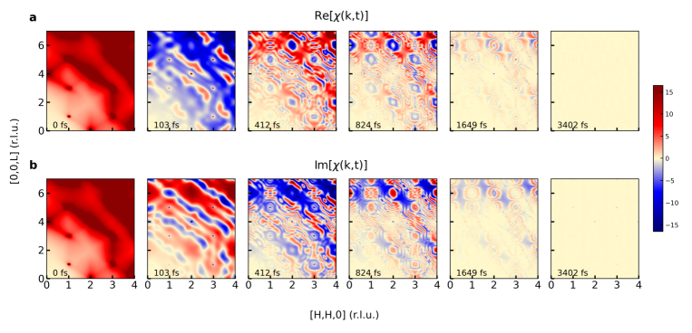
Figure 1: Response function $\chi(\mathbf{k},t)$ at different instances. Snapshots of (a) real and (b) imaginary parts of $\chi(\mathbf{k},t)$ at 0, 103, 412, 824, 1649 and 3402 femtoseconds (fs). $\chi(\mathbf{k},t)$ is shown in the $(H,H,L)$ reciprocal plane. The contour plots are normalized to their maximum intensity. The lattice dynamics dies out at longer time instances.

Figure 1 represents snapshots of the real and imaginary parts of the normalized $\chi(\mathbf{k},t)$ in the upper and lower panels, respectively. The dynamics can be seen as induced by the point-like source in ${\bf x}$, ⁴² akin to the nucleation site in electron microscopy imaging. From this point-like source term, silicon absorbs the energy at $t=0$, and phonon modes are generated in the entire reciprocal space (localized source in ${\bf x}$ is delocalized in ${\bf k}$). The snapshots are shown in the $(H,H,L)$ reciprocal plane for different time instances. We note that a (weak) optical pump pulse will also lead to the same $\chi(\mathbf{k},t)$ snapshots, as the pump pulse will generate first- and second-order states in the entire reciprocal space. The first-order disorder-activated continuum is generated in the absence of perfect crystalline order ³⁴. In contrast, the second-order squeezed states are generated by the coupling of a photon (momentum ${\bf q}\simeq 0$) with the two phonon modes of near-equal and opposite momenta (i.e., at $\mathbf{k}$ and $\mathbf{-k}$ due to the conservation of momentum) ³⁵. Thus in the present study, the simulated snapshots can be considered to arise from either a point-like source in ${\bf x}$ or generation of first- and second-order states. As evident from Fig. 1, these generated phonons propagate through the system and decay at different times for different $\mathbf{k}$ points according to their lifetime. It is possible to extract the lifetime of these phonon modes at different $\mathbf{k}$ values from the real and imaginary parts of the normalized $\chi(\mathbf{k},t)$ as we discuss below.

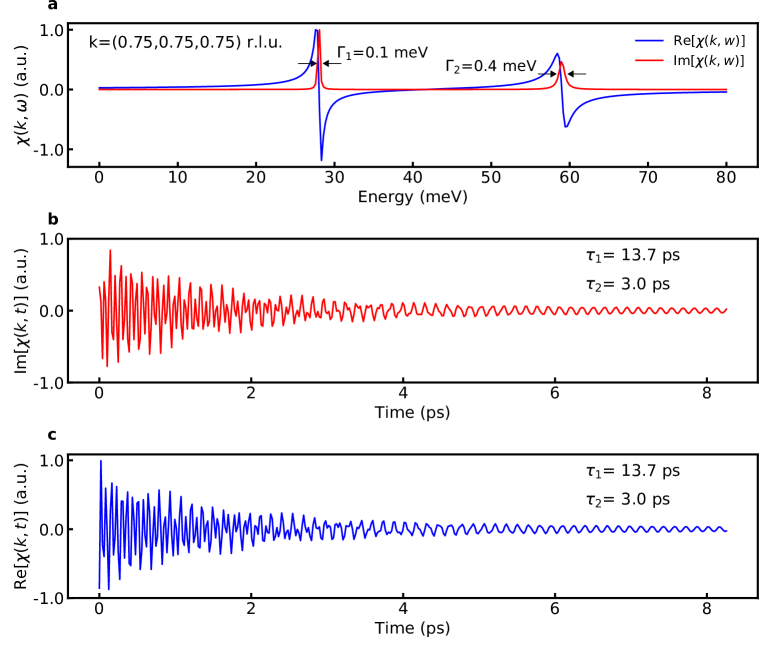
Figure 2: Decay width and lifetime of phonon modes at particular $\mathbf{k}$ point. (a) Real and imaginary parts of $\chi(\textbf{k},\omega)$ at particular $\mathbf{k}=(0.75,0.75,0.75)$ r.l.u. The decay widths corresponding to two active modes are $\Gamma_{1}=0.1$ meV and $\Gamma_{2}=0.4$ meV. (b) Imaginary part of $\chi(\textbf{k},t)$, which provides the lifetimes of the active phonon modes as $\tau_{1}=13.7$ ps and $\tau_{2}=3.0$ ps. (c) Real part of $\chi(\textbf{k},t)$, which gives the same values of the lifetimes of the active phonon modes. All the quantities plotted in sub-plots are normalized.

The real and imaginary parts of $\chi(\textbf{k},\omega)$ at a particular $\mathbf{k}=(0.75,0.75,0.75)$ r.l.u. is presented in Fig. 2a. Because of the phonon polarization factor ¹, at this particular $\mathbf{k}$ value, two phonon modes have finite intensity at energy values $\omega_{1}$= 28 meV (longitudinal acoustic) and $\omega_{2}$=60 meV (longitudinal optic). The full width at half maximum (FWHM) at these two energy values are $\Gamma_{1}=0.1$ meV and $\Gamma_{2}=0.4$ meV (obtained from first-principles simulation of Silicon ⁴³), which are known as decay widths of these modes. To extract the lifetime of these modes, $\chi(\textbf{k},t)$ is calculated from $\chi(\textbf{k},\omega)$. The imaginary and real parts of $\chi(\textbf{k},t)$ are shown in Figs. 2b and c, respectively. The lifetime ($\tau$) of both the active modes is obtained by fitting the exponentially decaying sinusoidal oscillation at the given $\mathbf{k}$ value, and are $\tau_{1}=13.7$ and $\tau_{2}=3.0$ ps. The fitted $\tau$ values are consistent with the values expected form its inverse relationship with $\Gamma$, i.e., $\Gamma=1/\pi\tau$, confirming the accuracy of our implementation. Also, the interferences visible in Figs. 2b and c are due to the presence of two active modes.

Till now, we have discussed dynamics induced by the point-like disturbance in ${\bf x}$, or first- and second-order states that lead to the excitation of all phonon modes in the reciprocal space. Let us analyze how $\chi(\textbf{k},t)$ manifests when the extended source in ${\bf x}$ induces the dynamics, which excites the phonon modes active at a single $\mathbf{k}$ value. A general time-dependent extended external source $n_{ext}({\bf x},t)$ can be treated as a Gaussian envelop in the ${\bf k}$-$\omega$ domain with standard deviation $\sigma$ controlling the spatial extent of the source. The induced dynamics $n_{ind}$ can subsequently be modeled as

$$n_{ind}(\mathbf{k},\omega)=\frac{4\pi}{k^{2}}\frac{1}{\sqrt{2\pi\sigma^{2}}}~{}\textrm{exp}{[{-(\mathbf{k}-\mathbf{k_{0}})^{2}}/{2\sigma^{2}}]}~{}\chi(\mathbf{k},\omega),$$ (2)

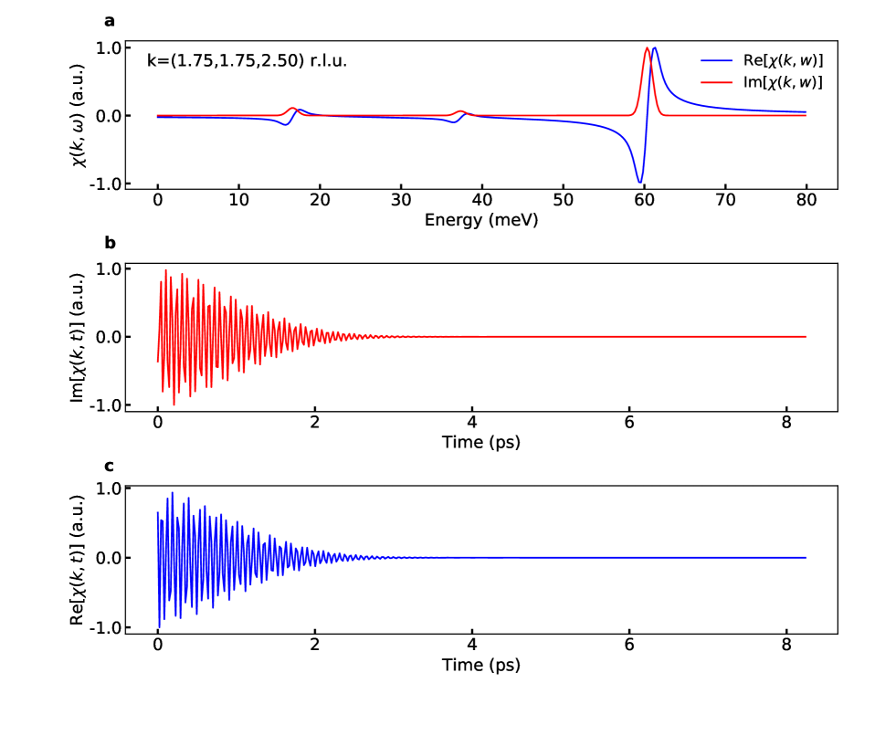
Figure 3: Decay width and dynamics of phonon modes excited by an extended source in ${\bf x}$. (a) Real and imaginary parts of $\chi(\textbf{k},\omega)$. (b) Imaginary and (c) real parts of $\chi(\textbf{k},t)$. Here, the phonon modes at a specific $\mathbf{k}$ value of $\mathbf{k_{0}}=(1.75,1.75,2.50)$ r.l.u. are excited by an extended source in ${\bf x}$. All the quantities plotted in sub-plots are normalized.

where $\mathbf{k_{0}}$ is the mean $\mathbf{k}$-value at which phonons are excited. The real and imaginary parts of $\chi(\textbf{k},\omega)$ at $\mathbf{k_{0}}=(1.75,1.75,2.50)$ r.l.u. showing finite intensity for the three phonon modes are shown in Fig. 3a. Since momentum transfer ${\bf k}$ and phonon wavevector ${\bf q}$ at $\mathbf{k_{0}}$ are not entirely parallel or perpendicular to each other, the three modes have mixed transverse and longitudinal character. We emphasize that for an infinitely extended source as considered here, dynamics at all other ${\bf k}$ points are zero. As one can observe from Figs. 3b and c, finite line-widths of the phonon modes allow them to decay in few picoseconds. Note that we do not explicitly include the phonon scattering channels in our approach. When included, these scattering channels will increase the phonon population with time at other ${\bf k}$ points that satisfy the momentum and energy conservation ^{17; 36; 37}.

II.3 Response function and time-resolved diffuse x-ray scattering

To know how well-grounded the discussed method of extracting $\chi(\mathbf{k},t)$ from $S(\mathbf{k},\omega)$ (obtained from inelastic scattering measurements or simulations) is, we will compare our simulated results with the measured $\chi(\mathbf{k},t)$. Trigo et al. have performed time-resolved diffuse x-ray scattering on germanium ¹⁷. In that experiment, an optical pump pulse of 800 nm with a nominal width of 50 fs was used to generate correlated pairs of phonons with equal and opposite momenta at ${\bf k}$ and ${\bf-k}$, i.e., the squeezed states having $\langle{u}(t)\rangle=0$. Here $u$ is the atomic displacement, and $t$ denotes the pump-probe delay time. A 50 fs x-ray pulse having 10 keV photon energy from Linac Coherent Light Source (LCLS) was used to probe diffuse scattering from the squeezed states at various pump-probe delay times. The temporal evolution of the equal-time correlation function was probed ¹⁷. Due to the time-resolved nature of the experiment, the time evolution of the squeezed states and the anharmonic decay of phonons is seen in the ${\bf k}$-$t$ domain. Note that for the squeezed states, the diffuse scattering intensity oscillates at twice the phonon frequency ¹⁷.

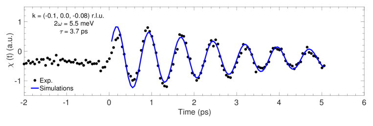
Figure 4: Comparison of experimental data with simulated $\chi(t)$ for germanium. Normalized difference intensity of the diffuse scattering at $\mathbf{k}=(-0.10,0.00,-0.08)$ r.l.u. is from the experiment presented in Ref. 17 (black color), and our simulated $\chi(t)$ is shown by blue color.

Figure 4 presents the comparison of the experimental data from Ref. 17 with our simulated result of $\chi(\mathbf{k},t)$ for germanium. To demonstrate the merit of our work, we have chosen the data at $\mathbf{k}=(-0.10,0.00,-0.08)$ r.l.u. only. Since $\chi(\mathbf{k},t)$ is dependent on the phonon mode polarization, the calculated intensity at $\mathbf{k}$ is due to the oscillations at $2\omega\sim$ 5.5 meV. In the experiment, the normalized difference intensity was shown, which provides the time-resolved value of the equal-time correlation function at $\mathbf{k}$ and $\mathbf{-k}$ ¹⁷. As reflected from the figure, the present simulated result is an excellent agreement with the experimental data for $\tau\sim$ 3.7 ps. Such a large value of $\tau$ for dispersive phonon modes, which is straightforward to obtain from ${\bf k}$-$t$ domain measurements, is not so easy to extract from INS or IXS measurements owing to the finite instrument resolution in ${\bf k}$ and $\omega$ ^{29; 30; 31}.

In spite of the excellent agreement, an important question arises: how the two different methods – time-resolved diffuse x-ray scattering and inelastic x-ray scattering, yield the same information. In Ref. 17, it is mentioned that time-resolved diffuse x-ray scattering probes equal-time density-density correlation function: $\langle\hat{n}(\mathbf{-k},t)~{}\hat{n}(\mathbf{k},t)\rangle$ with $\hat{n}$ as a density operator ^{44; 45}. On the other hand, it is well-established that inelastic x-ray scattering probes density-density correlation function at different time: $\langle\hat{n}(\mathbf{-k},t)~{}\hat{n}(\mathbf{k},0)\rangle$, which is related to the Van Hove correlation function ^{3; 42; 46}. However, there is no contradiction as the experiment was performed without energy resolution and the presented data were energy integrated ¹⁷. The density-density correlation function at different time, probed by inelastic x-ray scattering, reduces to equal-time density-density correlation function in the case where energy resolution is lacking. Therefore, without energy resolution, time-resolved diffuse x-ray scattering and inelastic scattering yield identical information: $\langle\hat{n}(\mathbf{-k},t)~{}\hat{n}(\mathbf{k},t)\rangle$, apart from a pre-factor (see Supplementary Material for derivation).

II.4 Response function in real-space

Not only time-resolved scattering methods in a pump-probe configuration provide the temporal evolution of correlation function, but also help us to visualize atomic motion (lattice dynamics) in the ${\bf x}$-$t$ domain ^{12; 13}, for example, as in the time-resolved electron microscopy experiments ^{25; 26; 33}. In the following, we demonstrate that momentum and energy-resolved inelastic scattering signal also provides the snapshots of the lattice dynamics in the ${\bf x}$-$t$ domain. For this purpose, we need to perform one more Fourier transform from momentum space to real space to obtain $\chi(\textbf{x},t)$ from $\chi(\textbf{k},t)$. Following Fourier relation, the spatial resolution along the $[H,H,0]$ direction is estimated as $\Delta\mathbf{x}={2\pi}/({6.5}$ Å${}^{-1})$ = 0.96 Å , whereas along the $[0,0,L]$ direction is $\Delta\mathbf{x}={2\pi}/({8.1}$ Å${}^{-1})$ = 0.78 Å. The spatial extent of the dynamics ranges from $(0,0)$ to $(153,108)$ Å. Similar to the time resolution and duration, the spatial resolution and extent are governed by momentum transfer and momentum resolution of the measurements/simulations.

The snapshot of $\chi(\textbf{x},t)$ indicates how and where the disturbance, imparted at $t=0$, has travelled in real space. $\chi(\textbf{x},t)$ at $t$ = 400 fs in the $(H,H,L)$ plane is shown in Fig. 5. In this case, the dynamics is induced by a point source at ${\bf x}=(0,0,0)$ in silicon. As silicon crystal is anisotropic; therefore the phonon propagation is not spherical as generally assumed for the scattering of light waves from a point-like source. Instead, the anisotropic phonon group velocity governs the 3D extent of energy re-distribution after time $t$. The extent of disturbance along a particular direction at any given time can be estimated from the maximum velocity given by the dispersion of longitudinal acoustic mode at the zone-center. In the present case, the maximum velocity along the $[H,H,0]$ direction is 8958 ms^-1, whereas it is 8381 ms^-1 along the $[0,0,L]$ direction.

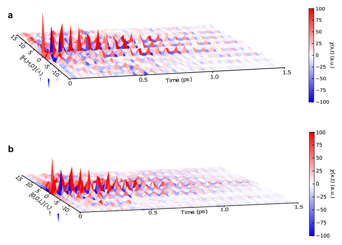
Figure 6: Visualization of the lattice dynamics induced by a point source in silicon in the $({\bf{x},t})$ domain. The dynamics (a) along the $[1,1,0]$ direction and (b) along the $[0,0,1]$ direction. The disturbance is still in the system at large instances, but the ripples’ height is low. There is no dissipation of energy from the system.

Figure 6 presents the entire dynamics along $[1,1,0]$ and $[0,0,1]$ directions in upper and lower panels, respectively. Before the disturbance at $t<0$, the system is in equilibrium. At $t=0$, the system is struck with a negative disturbance. As a result of this disturbance, a positive recoil at the origin is generated, surrounded by a minimal positive build-up. As visible from the figure, the density-induced disturbance is propagating through the entire system as time evolves. At large time instances, the disturbance is still into the system, but the order is minimal due to the spread of energy into the system (no dissipation of energy from the system). Such time-resolved images can be captured nowadays using real-space femtosecond electron imaging, as recently demonstrated for the phonon nucleation and launch at a crystal step-edge in the WSe₂ flake ²⁶. At this point, it is important to mention that Abbamonte and co-workers have employed a similar reconstruction method of $\chi(\mathbf{x},t)$ from inelastic x-ray scattering data to visualize electron dynamics in various systems ^{41; 47; 48}.

II.5 Practical challenges

Despite the applicability of our approach to inelastic scattering methods, we should keep experimental and data analysis limitations in mind. For example, 4D momentum-, crystallographic direction-, and energy-resolved datasets of lattice dynamics are presently feasible with high-resolution ($\sim$1 meV, or better) INS and IXS ^{29; 30; 31}. In EELS, the energy resolution may always not be suitable for low energy phonons ($<$  30 meV), as intense zero-loss peak masks the spectrum ^{49; 50}. Even in INS and IXS measurements, the scattering intensity varies among elements. Since x-ray scattering cross-section increases with the atomic number $Z$, phonon intensity of low $Z$ elements is considerably weak. Moreover, acquiring a complete 4D dataset using IXS with an array of monochromators will require a long measurement time (several days, as measurements at a few momentum transfers generally take 15 to 120 minutes). Similarly, in INS, several elements have small coherent scattering cross-section (i.e., H, V, Co) or high absorption coefficient (i.e., B, Cd); thus, phonon dispersion measurements remain challenging in materials with these elements. INS measurements also have kinematic constraints (all momentum and energy transfer are not accessible), and energy resolution, instead of being a constant number, depends on the phonon energy ^{1; 2}. Deconvolution of energy resolution from the measured 4D dataset to extract the intrinsic details, for example, $\tau$, is not always straightforward ⁵¹. Recent advances in experimental techniques and data analysis are overcoming many of the limitations. Together with simulations, they can provide full or complementary information, as demonstrated in this study.

In summary, we have established that inelastic scattering methods have potential to image lattice dynamics with atomic-scale spatiotemporal resolution. Few tens of femtoseconds temporal and $\sim 1$ Å spatial resolutions can be achieved during the reconstruction of lattice dynamics by utilizing the superior energy and momentum resolutions of inelastic scattering measurements. Our proposed theoretical method allows for direct imaging of lattice dynamics and enables us to extract the lifetime of selective phonon modes. Moreover, there is a flexibility to decide whether a single phonon mode or several phonon modes participate in the dynamics by choosing the disturbance source’s spatial extent in the real-space. The excellent agreement between the present simulated result and the measured lattice dynamics in germanium provides confidence and robustness of the proposed method. We believe that the current approach will be an alternative to time-resolved diffraction methods to image lattice dynamics and beneficial to the situations where time-resolved diffraction is not easy to perform, such as neutron scattering and in-situ measurement conditions.

III Methods

III.1 Dynamical structure factor calculation

The dynamical structure factor $S(\mathbf{k},\omega)$ was calculated using the following expression:

$$S(\mathbf{k},\omega)\propto \sum_{s}\sum_{\mathbf{\tau}}\frac{1}{\omega_{s}}\left|\sum_{d}\frac{{f_{d}({\bf k})}}{\sqrt{M_{d}}}\rm{exp}(-W_{d})\rm{exp}(i\mathbf{k}\cdot\mathbf{d})(\mathbf{k}\cdot\mathbf{e}_{ds})\right|^{2}\times\langle n_{s}+\frac{1}{2}\pm\frac{1}{2}\rangle\delta(\omega\mp\omega_{s})\delta(\mathbf{k}-\mathbf{q}-\mathbf{\tau}),$$ (3)

where $f_{d}({\bf k})$ is the form factor for atom $d$ (can be replaced by the neutron scattering length $\overline{b_{d}}$ for inelastic neutron scattering), k = k’ - k” is the wavevector or momentum transfer, and k” and k’ are the final and incident wavevector of the scattered particle, respectively; q is the phonon wavevector, $\omega_{s}$ is the eigenvalue and $\mathbf{e}_{ds}$ is the eigenvector of the phonon corresponding to the branch index $s$, $d$ is the atom index in the unit cell, $\tau$ is the reciprocal lattice vector, $\exp(-2W_{d})$ is corresponding to the Debye-Waller factor, and $n_{s}=\left[\exp\left(\frac{\hbar\omega_{s}}{k_{\rm B}T}\right)-1\right]^{-1}$ is the Bose-Einstein occupation factor. The $+$ and $-$ sign in Eq. (3) correspond to phonon creation and phonon annihilation, respectively. The phonon eigenvalues and eigenvectors (simulation details are same as presented in Refs. 38 and 39) in Eq. (3) were obtained by solving dynamical matrix using Phonopy ⁵². Phonon dispersion curves, $S(\mathbf{k},\omega)$ and constant energy slices of $S(\mathbf{k},\omega)$ of silicon and germanium are given in Supplementary Information.

Data Availability

Data that support the plots within this paper and other findings of this study are available from the corresponding authors upon reasonable request.

Code Availability

Code that support the findings of this study are available from the corresponding authors on reasonable request.

Author Contributions

D.B. and G.D. conceived the idea, designed the research, and supervised the work. N.R. and A.P.R. performed simulations. All authors discussed the results and contributed to the final manuscript. D.B. and G.D. wrote the manuscript.

Competing Interests

The authors declare no competing interests.

Figure 5: Snapshot of $\chi(\mathbf{x},t)$ in the $(H,H,L)$ plane at $t$ = 400 fs for silicon. The dotted lines represent the extent to which there are disturbances in $[1,1,0]$ and $[0,0,1]$ directions, which is given by the dispersion of longitudinal acoustic mode at the zone-center.

References

- (1) Squires, G. Introduction to the theory of thermal neutron scattering (Cambridge University Press, 1978).
- (2) Willis, B. & Carlile, C. Experimental Neutron Scattering (Oxford University Press, Oxford, 2009).
- (3) Schülke, W. Electron dynamics by inelastic X-ray scattering. 7 (Oxford University Press, 2007).
- (4) Egerton, R. F. Electron energy-loss spectroscopy in the electron microscope (Springer Science & Business Media, 2011).
- (5) Niedziela, J. et al. Selective breakdown of phonon quasiparticles across superionic transition in CuCrSe2. Nature Physics 15, 73–78 (2019).
- (6) Lindsay, L. & Polanco, C. A. Thermal transport by first-principles anharmonic lattice dynamics. Handbook of Materials Modeling: Applications: Current and Emerging Materials 735–765 (2020).
- (7) Dove, M. Introduction to Lattice Dynamics (Cambridge University Press, Cambridge, 1993).
- (8) Fultz, B. Vibrational thermodynamics of materials. Progress in Materials Science 55, 247–352 (2010).
- (9) Bansal, D. et al. Phonon anharmonicity and negative thermal expansion in SnSe. Physical Review B 94, 054307 (2016).
- (10) Bansal, D. et al. Momentum-resolved observations of the phonon instability driving geometric improper ferroelectricity in yttrium manganite. Nature Communications 9, 15 (2018).
- (11) Bansal, D. et al. Magnetically driven phonon instability enables the metal–insulator transition in h-FeS. Nature Physics 16, 669–675 (2020).
- (12) Gaffney, K. J. & Chapman, H. N. Imaging atomic structure and dynamics with ultrafast x-ray scattering. Science 316, 1444–1448 (2007).
- (13) Sciaini, G. & Miller, R. J. D. Femtosecond electron diffraction: heralding the era of atomically resolved dynamics. Reports on Progress in Physics 74, 096101 (2011).
- (14) Hartmann, N. et al. Attosecond time–energy structure of x-ray free-electron laser pulses. Nature Photonics 12, 215 (2018).
- (15) Emma, P. et al. First lasing and operation of an ångstrom-wavelength free-electron laser. Nature Photonics 4, 641–647 (2010).
- (16) Morimoto, Y. & Baum, P. Diffraction and microscopy with attosecond electron pulse trains. Nature Physics 14, 252–256 (2018).
- (17) Trigo, M. et al. Fourier-transform inelastic x-ray scattering from time-and momentum-dependent phonon–phonon correlations. Nature Physics 9, 790–794 (2013).
- (18) Clark, J. et al. Ultrafast three-dimensional imaging of lattice dynamics in individual gold nanocrystals. Science 341, 56–59 (2013).
- (19) Elsaesser, T. & Woerner, M. Perspective: Structural dynamics in condensed matter mapped by femtosecond x-ray diffraction. Journal of Chemical Physics 140, 020901 (2014).
- (20) Bredtmann, T., Ivanov, M. & Dixit, G. X-ray imaging of chemically active valence electrons during a pericyclic reaction. Nature communications 5, 1–7 (2014).
- (21) Fritz, D. M. et al. Ultrafast bond softening in bismuth: Mapping a solid’s interatomic potential with x-rays. Science 315, 633–636 (2007).
- (22) Siwick, B. J., Dwyer, J. R., Jordan, R. E. & Miller, R. J. D. An atomic-level view of melting using femtosecond electron diffraction. Science 302, 1382–1385 (2003).
- (23) Wall, S. et al. Atomistic picture of charge density wave formation at surfaces. Physical Review Letters 109, 186101 (2012).
- (24) Brown, S. B. et al. Direct imaging of ultrafast lattice dynamics. Science advances 5, eaau8044 (2019).
- (25) Flannigan, D. J. & Zewail, A. H. 4D electron microscopy: Principles and applications. Accounts of Chemical Research 45, 1828–1839 (2012).
- (26) Cremons, D. R., Plemmons, D. A. & Flannigan, D. J. Femtosecond electron imaging of defect-modulated phonon dynamics. Nature communications 7, 1–8 (2016).
- (27) Fu, X., Chen, B., Tang, J., Hassan, M. T. & Zewail, A. H. Imaging rotational dynamics of nanoparticles in liquid by 4d electron microscopy. Science 355, 494–498 (2017).
- (28) Pomerantz, I. et al. Ultrashort pulsed neutron source. Physical Review Letters 113, 184801 (2014).
- (29) Ehlers, G., Podlesnyak, A., Niedziela, J., Iverson, E. & Sokol, P. The new cold neutron chopper spectrometer at the spallation neutron source: Design and performance. Review of Scientific Instruments 82 (2011).
- (30) Stone, M. et al. A comparison of four direct geometry time-of-flight spectrometers at the spallation neutron source. Review of Scientific Instruments 85, 045113 (2014).
- (31) Said, A. H. et al. High-energy-resolution inelastic X-ray scattering spectrometer at beamline 30-ID of the advanced photon source. Journal of Synchrotron Radiation 27 (2020).
- (32) Wall, S. et al. Ultrafast disordering of vanadium dimers in photoexcited VO2. Science 362, 572–576 (2018).
- (33) Cremons, D. R., Plemmons, D. A. & Flannigan, D. J. Defect-mediated phonon dynamics in TaS2 and WSe2. Structural Dynamics 4, 044019 (2017).
- (34) Carles, R., Zwick, A., Renucci, M. & Renucci, J. A new experimental method for the determination of the one phonon density of states in gaas. Solid State Communications 41, 557–560 (1982).
- (35) Henighan, T. et al. Control of two-phonon correlations and the mechanism of high-wavevector phonon generation by ultrafast light pulses. Physical Review B 94, 020302 (2016).
- (36) Stern, M. J. et al. Mapping momentum-dependent electron-phonon coupling and nonequilibrium phonon dynamics with ultrafast electron diffuse scattering. Physical Review B 97, 165416 (2018).
- (37) Murphy-Armando, F. et al. Evolution of non-thermal phonon and electron populations in photo-excited germanium on picosecond timescales. arXiv preprint arXiv:1911.12145 (2019).
- (38) Bao, F., Archibald, R., Bansal, D. & Delaire, O. Hierarchical optimization for neutron scattering problems. Journal of Computational Physics 315, 39–51 (2016).
- (39) Bao, F., Archibald, R., Niedziela, J., Bansal, D. & Delaire, O. Complex optimization for big computational and experimental neutron datasets. Nanotechnology 27, 484002 (2016).
- (40) Jackson, J. D. Classical electrodynamics (John Wiley & Sons, 2007).
- (41) Abbamonte, P., Finkelstein, K. D., Collins, M. D. & Gruner, S. M. Imaging density disturbances in water with a 41.3-attosecond time resolution. Physical Review Letters 92, 237401 (2004).
- (42) Abbamonte, P. et al. Ultrafast imaging and the phase problem for inelastic x-ray scattering. Advanced Materials 22, 1141–1147 (2010).
- (43) Carrete, J. et al. almabte: A solver of the space–time dependent boltzmann transport equation for phonons in structured materials. Computer Physics Communications 220, 351–362 (2017).
- (44) Dixit, G., Slowik, J. M. & Santra, R. Theory of time-resolved nonresonant x-ray scattering for imaging ultrafast coherent electron motion. Physical Review A 89, 043409 (2014).
- (45) Dixit, G., Vendrell, O. & Santra, R. Imaging electronic quantum motion with light. Proceedings of the National Academy of Sciences 109, 11636–11640 (2012).
- (46) Van Hove, L. Correlations in space and time and born approximation scattering in systems of interacting particles. Physical Review 95, 249–262 (1954).
- (47) Abbamonte, P. et al. Dynamical reconstruction of the exciton in lif with inelastic x-ray scattering. Proceedings of the National Academy of Sciences 105, 12159–12163 (2008).
- (48) Abbamonte, P., Reed, J. P., Joe, Y., Gan, Y. & Casa, D. Implicit spatial averaging in inversion of inelastic x-ray scattering data. Physical Review B 80, 054302 (2009).
- (49) Krivanek, O. L. et al. Vibrational spectroscopy in the electron microscope. Nature 514, 209–212 (2014).
- (50) Venkatraman, K., Levin, B. D., March, K., Rez, P. & Crozier, P. A. Vibrational spectroscopy at atomic resolution with electron impact scattering. Nature Physics 15, 1237–1241 (2019).
- (51) Lin, J. Y. et al. MCViNE–an object oriented monte carlo neutron ray tracing simulation package. Nuclear Instruments and Methods in Physics Research Section A: Accelerators, Spectrometers, Detectors and Associated Equipment 810, 86–99 (2016).
- (52) Togo, A. & Tanaka, I. First principles phonon calculations in materials science. Scripta Materialia 108, 1–5 (2015).