Single-preparation unsupervised quantum machine learning: concepts and applications

Abstract

The term “machine learning” especially refers to algorithms (and associated systems) that derive mappings, i.e. intput/output transforms, by using numerical data that provide information about the transform of interest in the considered application. The data processing tasks to be performed in these applications not only include classification/clustering and regression, but also various problems related to system identification, system inversion and input signal restoration or source separation (i.e. signal separation) when considering several signals. In this paper, we first analyze the connections that exist between all these problems, in the classical and quantum frameworks. We then focus on their most challenging versions, where quantum data and/or quantum processing means are considered and learning is performed in the unsupervised mode, also called the blind mode, i.e. without “reference values” (at the input or output of the mapping, depending on the considered task). Moreover, we propose the quite general concept of SIngle-Preparation Quantum Information Processing (SIPQIP). The term “preparation” refers to the initialization of qubit states. As explained in the introduction, it is here used in a more general sense than usually in quantum mechanics: we mainly consider kets with random-valued coefficients. The resulting methods only require one to estimate expectations of probabilities of measurement outcomes associated with considered states. This may be achieved with a single instance of each state in our SIPQIP framework. This avoids the burden of usual methods, that have to very accurately create many copies of each fixed state, to estimate statistical features associated with that state. We detail or discuss the application of this SIPQIP concept to various tasks and systems that fulfill quantum mechanical principles, related to system identification (blind quantum process tomography or BQPT, blind Hamiltonian parameter estimation or BHPE, blind quantum channel identification/estimation, blind phase estimation), system inversion and state estimation (blind quantum source separation or BQSS, blind quantum entangled state restoration or BQSR, blind quantum channel equalization) and classification. Part of these methods are detailed for a specific class of quantum processes, which then allows one to extend them to other processes. These processes correspond to two qubits implemented as electron spins 1/2, internally coupled according to the cylindrical-symmetry Heisenberg model, with unknown principal values for the exchange tensor. The resulting numerical performance of these methods is reported, thus showing that the proposed SIPQIP framework moreover yields much more accurate estimation than the standard multiple-preparation approach, for a given total number of state preparations. Several types of proposed methods are especially of interest when used in a quantum computer, that we propose to more briefly call a “quamputer”: BQPT and BHPE simplify the characterization of the gates of quamputers, whereas BQSS and BQSR allow one to design quantum gates that may be used to compensate for the non-idealities that may alter states stored in quantum registers. BQSS/BQSR moreover opens the way to the much more general concept of self-adaptive quantum gates, that could automatically adapt their behavior, according to predefined rules that would allow them to compensate for various non-idealities in quamputers.

I Introduction

Classical machine learning is currently a booming field [1] and various quantum machine learning extensions are also being considered [2, 3, 4, 5]. The processing tasks that involve data-driven learning not only include widespread classification/clustering [6, 7, 8, 1, 9, 3, 10] and regression [6, 7, 9], but also especially: (a) classical system identification [11, 12, 13] and its quantum extension, called (non-blind [14, 15, 16, 17, 18, 19, 20, 21, 22, 23] or blind [24, 25, 26]) quantum process tomography, (b) system inversion and signal restoration and (c) blind source separation (BSS) e.g. based on independent component analysis (ICA) [27, 28, 29, 30, 31, 32, 33] (with a close connection with principal component analysis [34, 35, 36]) and quantum extensions of BSS/ICA [37, 38, 39, 40, 41, 42]. Moreover, in various application fields, these tasks are given different names (see the summary in Table 1), especially channel identification or channel estimation [12], (channel) equalization [12, 43], dereverbation [44], deconvolution [45], deblurring [45] or cocktail party problem [46].

	system identification	system inversion,
		signal restoration,
		source separation
classical	$\bullet$ channel identification,	$\bullet$ channel equalization
signals	channel estimation	(communication)
	(communication)	$\bullet$ deconvolution
	$\bullet$ impulse response	(image, seismology…)
	or transfer function	$\bullet$ dereverberation
	estimation	(acoustics)
	(acoustics…)	$\bullet$ cocktail party
		processing
		(audio)
		$\bullet$ deblurring
		(image)
quantum	$\bullet$ process tomography	$\bullet$ source separation
states	(Section IV.1)	(Section V.1)
	$\bullet$ Hamiltonian estimation	$\bullet$ state restoration
	(Section IV.2)	(Section V.2)
	$\bullet$ channel estimation	$\bullet$ channel equalization
	(Section IV.3)	(Section V.3)
	$\bullet$ phase estimation
	(Section IV.3)

Table 1: Application-dependent terminology of classical and quantum machine learning tasks (i.e. data-driven learning/adaptation methods) related to system identification, system inversion, signal restoration and source separation (apart from classification/clustering and regression). This yields non-blind and blind (i.e., supervised and unsupervised) variants. The sections of this paper mainly dealing with the blind (i.e., unsupervised) quantum single-preparation versions of these methods are mentioned.

Beyond their apparent diversity, the above data processing tasks share major features, that are analyzed in Section II: they involve mappings from input data to output data, and these mappings are derived from a set of known values of these input and/or output quantities, depending whether that learning is performed in the so-called supervised or unsupervised (i.e. non-blind or blind) modes, whose definitions depend on the considered task and are also analyzed in Section II. These approaches are developed in order to characterize the mapping performed by a given natural or artificial system, and/or in order to build an artificial system that performs a mapping (i.e. a data transformation) suited to the considered application.

In this paper, we investigate a variety of the above-defined data processing tasks and we focus on advanced configurations from the following points of view. First, we only consider a quantum framework, in terms of the nature of the data to be processed and/or of the means used to process them. Second, we almost only address unsupervised learning, which is more challenging than supervised learning because it consists of learning mappings without known values (but with a few known properties) for the input or output of that mapping. The overview of classical and quantum machine learning provided in Section II includes references to the currently quite limited set of works from the literature which is dedicated to that quantum and unsupervised learning framework that we tackle in this paper. Moreover, we here proceed beyond that framework, by adding another feature: we focus on what we call “single-preparation operation”. This concept is detailed in Section III. To put it briefly, various quantum machine learning methods from the literature, e.g. intended for system identification (i.e., say, quantum process tomography) or system inversion, use multiple-preparation approaches in the sense that, for each quantum state value that they consider, they estimate the probabilities of corresponding measurement outcomes by using the sample frequencies of these outcomes over a set of measurements, which requires a set of copies of the considered quantum state, to perform one measurement for each copy (see details in Section III.1). In contrast, we very recently introduced a statistical approach which yields much higher flexiblity, since it avoids the burden of very acccurately preparing many ideally identical copies of the same known state, by allowing one to replace these copies by a set of states whose values are possibly different and unknown but only requested to belong to a general known class [47, 26]. This concept is quite general but, in [47, 26], we only detailed its application to a single data processing task, namely single-preparation blind (i.e. unsupervised) quantum process tomography. In the present paper, we aim at showing how this single-preparation processing concept may be applied to a variety of other quantum information processing tasks of interest, thus yielding a general “SIngle-Preparation Quantum Information Processing” (SIPQIP) framework.

The terminology used in this paper deserves the following comments. Quantum mechanics (QM) considers that an isolated quantum system may be either in a pure state - the result of some preparation -, described by a ket with deterministic coefficients (in the Schrödinger picture), or more generally in a state called a mixed state or a statistical mixture, usually described by a density operator. When developing our methods, first in the BQSS then in the BQPT fields, we were led to distinguish between a “deterministic pure state” (the usual pure state of QM), and a “random pure state”, described by a ket with random-valued coefficients when developed over an orthonormal basis of fixed vectors. It has been shown that the system is then in a mixed state [48]. Deterministic pure states may also be considered as a specific subset of random pure states, corresponding to the case when the random variables that define the ket coefficients of random pure states reduce to fixed values, i.e. with “no uncertainty”. In the context of BQSS or BQPT, depending on the considered method, the system of interest is initialized either in a deterministic or in a random pure state. Most of the methods proposed in this paper are based on qubits initialized with random pure states. Such an initialization is also called a state preparation hereafter.

The remainder of this paper is organized as follows. In Section II, we first provide an overview of major classical and quantum machine learning tasks, and we analyze their connections, that are of interest for our subsequent original contributions in this paper. Then, in Section III, we define the single-preparation quantum processing concept, which is an original general feature then used in all processing methods proposed in this paper. These methods deal with various problems related to quantum system identification (Section IV), quantum system inversion and state restoration (Section V) and quantum classification (Section VI). Finally, Section VII contains conclusions about the processing tasks addressed in this paper and a discussion of potential extensions of the proposed methods to other quantum information processing problems.

II Classical and quantum machine learning approaches for data mapping

Many classical and quantum information processing systems aim at applying transforms, defined by mathematical functions, to their input data, in order to map them to output data. These transforms are often called mappings or maps, both in the classical [6] and quantum [49] information processing literature (quantum maps are also called quantum channels [49], with a reference to communications). In basic systems, the considered transform is predefined by the human system designer, depending on the target application. In contrast, more advanced systems, that are considered hereafter, are referred to as (self-)adaptive systems, since they adapt their behavior (i.e. the mapping they perform) to the data they receive [50, 51], by means of algorithms which perform so-called adaptation, training or (machine) learning [6, 7, 8, 1, 9]. In other applications, input/output mappings are also learnt from data but with other goals, especially to characterize the behavior of a given natural medium or artificial system, as detailed below. The classical and quantum versions of machine learning thus involve various types of applications and associated types of transforms, that are analyzed in more detail hereafter.

Machine learning is first used in classical classification and regression systems, whose transforms map a set of input quantities (each of which has its own nature) to output quantities which often have a different nature from input ones. This is especially true for classification systems [6, 7, 8, 1, 9], which receive a set of input quantities that are most often continuous valued, whereas their (possibly thresholded) outputs are binary valued. More precisely, let us first consider a classification system without the rejection capability that is defined further. Such a system generally outputs $C$ values, where $C$ is the number of classes involved in the considered application. Only one of these outputs is equal to 1, say output with index $c$, whereas all other outputs are equal to 0. The index $c$ of the active output defines the decision made by the classifier: it considers that its input values correspond to a case when the input belongs to class $c$. During the final use of the classifier, called the “resolution phase”, “classification phase” or “test phase”, the above output values are provided to the target application. A typical use of this framework is Optical Character Recognition (OCR) [6, 8, 9]. The classifier then receives an image, i.e. a set of pixel values (or features, i.e. parameters, extracted from them), where a letter or symbol belonging to a given alphabet is written. The classifier sets its $c$-th output to 1 if it considers that this particular input image contains the $c$-th symbol of that alphabet. Moreover, improved classification algorithms are able to detect when they consider that the input that they receive during the resolution phase does not belong to any of the considered classes, e.g. when the received image is not similar enough to any character of the considered alphabet (indeed, an image may contain a shape which is not a character of any written language). Such a classifier then decides that it is not able to classify the considered input “object” and it rejects it. This may be expressed e.g. by setting all $C$ outputs to zero or by adding a $(C+1)$-th output to the classifier, which is equal to 1 when this classifier succeeds in classifying the considered input and to 0 otherwise.

Before the above resolution phase, machine learning algorithms are typically used, e.g. in OCR systems, to initially build an adequate input-output mapping, during the so-called “learning phase”, “training phase” or “adaptation phase” (this possibly includes a so-called “validation”), by using data composed of training examples. In supervised learning approaches, each example consists of an input (e.g., an image containing a character for OCR) and its correct class, i.e. the associated desired values of the classifier outputs (called labels), which are provided by a supervisor, i.e. typically a human expert of the considered application. In contrast, in unsupervised learning approaches for classification (called clustering [9]), the system self-organizes by using only inputs (e.g., images in the OCR example), i.e. unlabeled data. Various system architectures and supervised or unsupervised learning algorithms have thus been developed, especially including (artificial) neural networks [6, 7, 8, 9] and their recent deep extensions [1], as well as Support Vector Machines (SVM) [7, 8, 9].

Regression systems [6, 7, 9] are similar to the above classifiers, except that their outputs are continuous-valued. They typically first use a supervised training phase in order to learn mappings from data samples, which are examples of adequate pairs composed of input values and correct corresponding output values in the considered applications. Once this mapping has been fixed, such a regression system may eventually be used e.g. to control an industrial setup in a factory: the regression system then receives, as its inputs, different types of measured quantities provided by sensors available in the factory, and this system maps its inputs to possibly different types of continuous-valued quantities, used to drive the actuators that control the industrial setup. More specifically, regression systems where the inputs and output(s) have the same nature especially concern prediction tasks for time series, where the system aims at providing the expected future value(s) of a quantity (e.g. a currency exchange rate or streamflow) from its past values.

Whereas the above concepts were initially developed for classical data, they are currently being extended to quantum data and/or quantum processing means [3], especially because the Quantum Information Processing (QIP) [14] community is investigating quantum extensions of classifiers to handle the huge processing power and amount of data involved in current real-world applications. These extensions include the implementation of SVM classifiers on quantum computers with very low computational complexity [10]. Besides, the versatile quantum optical neural networks proposed in [52] can perform different related tasks, including reinforcement learning.

Although one may first have in mind the above general classification and regression/prediction tasks when thinking of classical and quantum machine learning, data-driven algorithms are also widely used in a partly related set of processing tasks, called system identification and system inversion, with an extension to source separation. First considering the classical framework, this e.g. includes situations when an electromagnetic or acoustic signal is emitted from a first location, then transferred through a medium, which may be seen as an electromagnetic or acoustic “channel” that transforms its input composed of the emitted signal. The output of that channel is then the signal received by an electromagnetic antenna or microphone in a second location. These and other practical situations yield two types of machine learning problems. The first one is often called system identification [11, 12, 13], and more specifically channel identification or channel estimation in the field of electromagnetic communications [12]. Its simpler version [13], called the “non-blind version” by the signal and image processing community and the “supervised version” by the machine learning and data analysis community, operates as follows. As in the above regression task, it uses a set of known continuous-valued pairs composed of input values and corresponding output values of the considered “system”, i.e. of the above-defined channel, in order to estimate, i.e. learn, the unknown transform (i.e. mapping) performed by this system. It should be noted that, in the above examples involving electromagnetic or acoustic signals, the considered “‘system” is not an artificial system to be built by human beings in order to perform a given type of data processing (as in the above classification and regression tasks), but the “natural system” formed by the considered electromagnetic or acoustic propagation medium. The goal of system identification is then to characterize this medium.

System identification methods have also been extended to the more challenging blind, i.e. unsupervised, configuration [11, 12]. In that case, during the learning or estimation phase, only the values of the system output (i.e. the values of the received channel output in the above examples) are known, whereas its input values are unknown. However, the system input is most often required to have some known properties, e.g. some known statistical features, so that this configuration is sometimes stated to be semi-blind or semi-supervised. This problem may therefore be seen as a non-conventional form of regression, with only partial knowledge about the input data. Besides, it should be noted that the known values are only the output values in blind system identification, whereas they are only the input values in the above unsupervised classification problem. Whereas non-blind or blind system identification is applied to single-input single output (SISO) systems in its basic form, it may then be extended to multiple-input multiple-output (MIMO) systems.

The second considered machine learning problem, in connection with system identification, deals with system inversion and signal restoration. One then again considers an unknown “system”, called the direct system, but one here aims at building an artificial system that essentially performs a transform equal to (an estimate of) the inverse of that of the direct system (assuming that direct transform is invertible). This inverse transform is first learnt during the training/adaptation phase, either directly or by first learning the direct transform (using system identification methods) and then deriving its inverse (in low-noise scenarios). Then, in the “inversion phase”, which corresponds to the final use of the inversion system, the (estimated) inverse transform is applied to known output values of the direct system, in order to recover (estimates of) corresponding unknown input values of that direct system. This approach e.g. applies to the above two configurations involving channels. The direct system then corresponds to the physical propagation medium, such as an electromagnetic communication channel, which alters the emitted signal in a initially unknown way. One then aims at restoring the emitted signal from its altered received version, by learning an adequate inverse transform from data samples. In the field of radio-frequency communications, this signal processing task is often referred to as (channel) equalization [12, 43]. Similarly, the restoration of an unknown emitted acoustic signal from its received version altered by reverberation during propagation is often called dereverbation [44]. More generally speaking, the problem of restoring a source signal only from an observation which is a transformed version of that source signal is called deconvolution (for a linear invariant transform) or deblurring in various fields, such as astronomical image analysis [45]. Whatever the considered application field, the initial learning procedure for estimating the inverse transform may be applied in the non-blind or blind mode, i.e. respectively with known or unknown input values for the direct system, whereas the output values of that system are known in both modes. This “(unknown) system inversion” task may also be extended to MIMO configurations, in order to restore a set of unknown signals from a set of their transformed versions.

The blind MIMO system inversion problem is also closely related to the field of blind source separation (BSS) [27, 28, 29, 30, 31, 32, 33], whose quantum extension is one of the major topics tackled further in this paper, together with quantum extensions of system identification. In BSS, the goal is also to restore a set of unknown source signals from a set of available combinations of these signals (called mixtures in BSS), that result from an unknown transform which combines (i.e. mixes) these source signals. However, in BSS, one most often allows each restored signal to be equal to a source signal only up to an acceptable residual transform (called an indeterminacy), because such transforms cannot be avoided, due to the limited constraints that are set on the considered classes of signals and mixing transforms. When applied to the separation of acoustic/audio signals from their mixtures recorded by a set of microphones, BSS is often referred to as the “cocktail party problem” [46].

The first class of BSS methods that was developed and that is still of major importance is Independent Component Analysis, or ICA [29, 30, 31, 32]. ICA is a statistical approach, which essentially requires statistically independent random source signals. Thus, ICA is guaranteed to restore the source signals up to limited indeterminacies for the simplest class of mixtures, that is when the available signals are linear instantaneous (i.e. memoryless) combinations of the unknown source signals [29, 30, 31, 32]. For such mixtures, ICA may be seen as an extension of more conventional Principal Component Analysis, or PCA [34, 35].

PCA and ICA may both be used to perform mappings from the available $P$ variables to $P$ output variables that are linear instantaneous mixtures of these available variables. In other words, they yield a representation of the same data in a new basis. The selected bases are different in PCA and ICA. PCA uses one of the bases that are such that the output variables are uncorrelated. ICA uses one of the bases that are such that these output variables are statistically independent, which includes uncorrelatedness but is more constraining (for non-Gaussian signals). This is the reason why PCA alone cannot achieve BSS [32], but is often used as a first stage in ICA algorithms. Outside the framework of ICA, PCA is most often used as a mapping that projects the available data onto a lower-dimensional space, i.e. with dimension $D$ lower than $P$, by keeping only the first $D$ coordinates in the output basis, for visualization (with $D=2$, i.e. projection onto a plane, or $D=3$, i.e. 3-dimensional visualization) or compression tasks. Such a projection may also be used as a preprocessing stage of ICA, in order to reduce the influence of noise, when the available mixed signals contain noise and their number $P$ is higher than the number $M$ of source signals: one then keeps the first $D=M$ output components of PCA.

ICA also has connections with the above fields of classification and regression in the sense that a significant part of the algorithms developed in all these fields are based on the same class of tools, namely neural networks. More precisely, when initially developing ICA methods for linear instantaneous mixtures, one of the very first proposed approaches was the well-known Hérault-Jutten neural network (see e.g. [53, 54, 55, 56, 57] for its definition and analysis) and extended versions of that network were then introduced and analyzed (see e.g. [58, 59]). Neural approaches were then proposed for specific classes of nonlinear mixtures or without considering any restrictions on the type of mixture (see e.g. [60, 61, 62, 63]). Finally, the interest in neural methods recently raised again also in the field of BSS/ICA. For instance, generative adversarial networks (GANs) were used to perform linear and non-linear ICA [64].

The above connected fields of classical system identification, system inversion, (B)SS and PCA have been partly extended as follows to the quantum framework. Among these problems, the one which was first studied is the quantum version of non-blind system identification, especially introduced in 1997 in [66] and called “quantum process tomography” or QPT by the QIP community: see e.g. [14, 15, 16, 17, 18, 19, 20, 21, 22, 23]. The connection between non-blind system identification and regression (and hence, to a lower extent, classification), that we highlighted above, was by the way mentioned for the quantum framework in [67], which states “Quantum process tomography is able to learn an unknown function within well-defined symmetry and physical constraints - this is useful for regression analysis” and further considers “Regression based on quantum process tomography”.

The quantum version of the above-mentioned classical source separation, called Quantum Source Separation, or QSS, and especially its blind version, or BQSS, were then introduced in 2007 in [37]. Two main classes of BQSS methods were developed since then. The first one may be seen as a quantum extension of the above-mentioned classical ICA methods, since it takes advantage of the statistical independence of the parameters that define random source quantum states (qubit states). It is called Quantum Independent Component Analysis (or QICA, see e.g. [37],[38]) or, more precisely, Quantum-Source Independent Component Analysis (or QSICA, see e.g. [39]) to insist on the quantum nature of the considered source data, whereas it uses classical processing means (after quantum/classical data conversion). The second main class of BQSS methods was introduced in 2013-2014 in [40],[41] and then especially detailed in [42]. It is based on the unentanglement of the considered source quantum states and it typically uses quantum processing means to restore these unknown states from their coupled version. Independently from the above quantum extensions of BSS/ICA, a quantum version of PCA was introduced in 2014 in [36]. Finally, the blind extension of QPT was introduced in 2015 in [24] and then especially extended in [25] for its multiple-preparation version.

Indeed, the above blind or non-blind QPT and (B)QSS methods are restricted to “multiple-preparation” operation, as defined in Section I. Beyond these approaches, we hereafter proceed to the general “single-preparation” QIP (or SIPQIP) framework that may be built to obtain a more efficient operation and we then present its application to various QIP tasks.

III Single-preparation quantum information processing (QIP)

III.1 Multiple-preparation QIP

Let us consider an arbitrary number $Q$ of distinguishable [42] qubits, physically implemented as spins 1/2. If the quantum state $|\psi\rangle$ of this set of qubits at a given time is pure and deterministic, it belongs to the $2^{Q}$-dimensional space ${\cal E}$ defined as the tensor product of the 2-dimensional spaces respectively associated with each of the considered qubits. Moreover, this state reads

$$|\psi\rangle=\sum_{k=1}^{2^{Q}}c_{k}|{k}\rangle$$ (1)

where the vectors $|{k}\rangle$, with $k\in\{1,\dots,2^{Q}\}$, form the standard basis of ${\cal E}$, i.e. they are respectively equal to $|+\rangle_{1}\otimes|+\rangle_{2}\otimes\dots\otimes|+\rangle_{Q-1}\otimes|+\rangle_{Q}$ to $|-\rangle_{1}\otimes|-\rangle_{2}\otimes\dots\otimes|-\rangle_{Q-1}\otimes|-\rangle_{Q}$, where $|+\rangle_{j}$ and $|-\rangle_{j}$ form the standard basis of the state space associated with the qubit with index $j$ and $\otimes$ is the tensor product. The complex-valued coefficients $c_{k}$ are fixed and arbitrary, except that they meet the normalization condition

$$\sum_{k=1}^{2^{Q}}|c_{k}|^{2}=1.$$ (2)

When simultaneously measuring the spin components of all $Q$ qubits along the quantization axis, the obtained result is a vector of $Q$ values respectively associated with each of the qubits. That vector has a random nature and its $2^{Q}$ possible values (in normalized units) are $[+\frac{1}{2},+\frac{1}{2},\dots,+\frac{1}{2},+\frac{1}{2}]$, $[+\frac{1}{2},+\frac{1}{2},\dots,+\frac{1}{2},-\frac{1}{2}]$, and so on, these values being respectively associated with the basis vectors $|{k}\rangle$ and hereafter indexed by $k$. Thus, the experiment consisting of this $Q$-qubit measurement yields a random result, and each elementary event [68] $A_{k}$ is defined as: the result of the experiment is equal to the $k$-th $Q$-entry vector in the above series of possible values $[+\frac{1}{2},+\frac{1}{2},\dots,+\frac{1}{2},+\frac{1}{2}]$ and so on. Moreover, the probabilities of these events are equal to

$$P(A_{k})=|c_{k}|^{2}\hskip 28.45274pt\forall\ k\in\{1,\dots,2^{Q}\}.$$ (3)

The standard procedure, applied in practice to estimate the above probabilities for a given $Q$-qubit state, requires one to prepare a large number (typically from a few thousand up to a few hundred thousand [38, 42]) of copies of that state, so that we hereafter call this standard approach “multiple-preparation QIP” (this terminology and the connection between these methods and classical adaptive processing are discussed in Appendix A). These copies may be obtained in parallel from an ensemble of systems or successively for the same system (“repeated write/read”, or RWR, procedure [37, 38, 39]). The above type of measurement is performed for each of these copies and one counts the number of occurrences of each of the possible results $[+\frac{1}{2},+\frac{1}{2},\dots,+\frac{1}{2},+\frac{1}{2}]$ and so on. The associated sample relative frequencies are then used as estimates of the probabilities $P(A_{k})$.

As stated above, this approach requires many copies of the same quantum state. This is therefore constraining, especially in the framework of blind QIP, where the processing methods should operate with unknown values of some quantum states (e.g. unknown inputs of the process to be identified with QPT): being able to operate without requiring known values of quantum states in blind methods is attractive, but then requesting many copies of each such state to be available is still a limitation, because it still requires some form of control of these states, that we would like to avoid, in order to simplify the practical operation of the considered methods and to make them “blinder”. We hereafter provide a solution to this problem.

III.2 Single-preparation QIP based on probability expectations

The above description was provided for an arbitrarily selected deterministic pure quantum state $|\psi\rangle$. When developing our first class of BQSS methods (see e.g. [37, 38, 39, 48]) and associated BQPT methods (see e.g. [24, 25, 48]), we had to extend that framework to random pure quantum states. We especially detailed that concept in [48]. Briefly, the coefficients $c_{k}$ in (1) then become complex-valued random variables, instead of fixed parameters. Hence, the probabilities in (3) also become random variables!

The problem tackled in this section is the estimation of some statistical parameters of these random variables defined by (3), namely their expectations. The natural (global) procedure that may be used to this end, and that we used in our above-mentioned first BQSS and BQPT investigations, consists of the following two levels. The lower level only concerns one deterministic state (1) and the associated probabilities (3) which are estimated from a large number of copies of the considered state, using the multiple-preparation QIP framework of Section III.1. This is repeated for different states (1) and then, at the higher level, the sample mean over all these states is separately computed for each probability $P(A_{k})$ (with samples supposedly drawn from the same statistical distribution).

Beyond the above natural procedure, we hereafter focus on a more advanced approach, that we recently introduced in the short conference paper [47]. We then only partly described it and applied it to a single QIP task (namely BQPT) in the journal paper [26] whereas, in the present paper, we define it and analyze it in more detail and we then show that it also applies to a wide range of other QIP tasks. That modified procedure is based on the following principle: At the above-defined lower level, we aim at using a small number of copies of the considered state, or ultimately a single instance of that state, thus developing what we call “SIngle-Preparation QIP”or more briefly SIPQIP (this terminology and the connection between these methods and classical adaptive processing are also discussed in Appendix A). At first sight, it might seem that this is not possible, because the lower level would thus not provide accurate estimates, that one could then confidently gather at the higher level. However, we claim and show below that this approach can be used if one only aims at estimating some statistical parameters of the considered quantum states.

We now first build the proposed approach by starting from the frequentist view of probabilities (see e.g. [68]) at the above-defined two levels of the considered procedure, that is:

• At the higher level, where one combines the contributions associated with $N$ states of the set of $Q$ qubits. These states are indexed by $n\in\{1,\dots,N\}$ and denoted as $|\psi(n)\rangle$.

• At the lower level, which concerns one deterministic state $|\psi(n)\rangle$ and the associated probabilities $P(A_{k},n)$ defined by (3) but with coefficients $c_{k}(n)$ which depend on state $|\psi(n)\rangle$.

At the lower level, each probability $P(A_{k},n)$ is defined as

$$P(A_{k},n)=\lim_{K\rightarrow+\infty}\frac{{\cal N}(A_{k},n,K)}{K}$$ (4)

provided this limit exists. ${\cal N}(A_{k},n,K)$ is the number of occurrences of event $A_{k}$ for the state $|\psi(n)\rangle$ when performing measurements for a set of $K$ copies of that state $|\psi(n)\rangle$. In practice, one uses only a finite number $K$ of copies of state $|\psi(n)\rangle$ and therefore only accesses the following approximation of the above probability:

$$P^{\prime}(A_{k},n,K)=\frac{{\cal N}(A_{k},n,K)}{K}.$$ (5)

The higher level of the considered procedure then addresses the statistical mean associated with samples, indexed by $n$, of a given quantity, which is here theoretically $P(A_{k},n)$. In the frequentist approach, this statistical mean is defined (if the limit exists) as

$$E\{P(A_{k})\}=\lim_{N\rightarrow+\infty}\frac{\sum_{n=1}^{N}P(A_{k},n)}{N}.$$ (6)

At the higher level too, in practice one uses only a finite number $N$ of states $|\psi(n)\rangle$, which first yields the following approximation if only performing an approximation at the higher level of the procedure:

$$E^{\prime}\{P(A_{k})\}=\frac{\sum_{n=1}^{N}P(A_{k},n)}{N}.$$ (7)

The latter expression may then be modified by replacing its term $P(A_{k},n)$ by its approximation (5). This yields

$$E^{\prime\prime}\{P(A_{k})\}=\frac{\sum_{n=1}^{N}{\cal N}(A_{k},n,K)}{NK}.$$ (8)

$\sum_{n=1}^{N}{\cal N}(A_{k},n,K)$ is nothing but the number, hereafter denoted as ${\cal N}(A_{k},L)$, of occurrences of event $A_{k}$ for the complete considered set of $L=NK$ measurements. Therefore, $E^{\prime\prime}\{P(A_{k})\}$ is the relative frequency of occurrence of that event over these $L$ measurements, or “‘trials”, using standard probabilistic terms [68]. This quantity (8) may therefore also be expressed as

$$E^{\prime\prime}\{P(A_{k})\} = \frac{{\cal N}(A_{k},L)}{L}$$ (9)

$$= \frac{\sum_{\ell=1}^{L}11(A_{k},\ell)}{L}$$ (10)

where $11(A_{k},\ell)$ is the value of the indicator function of event $A_{k}$ for trial $\ell$, which takes the value 1 if $A_{k}$ occurs during that trial, and 0 otherwise. When using (10), one now considers the $L=NK$ trials as organized as a single series, with trials indexed by $\ell$. One thus fuses the above-defined two levels of the procedure into a single one, thus disregarding the fact that, in this series, each block of $K$ consecutive trials uses the same state $|\psi(n)\rangle$. One may therefore wonder whether the number $K$ of used copies of each state $|\psi(n)\rangle$ may be freely decreased, and even set to one, while possibly keeping the same total number $L$ of trials. A formal proof of the relevance of that approach, using Kolmogorov’s view of probabilities, is provided in Appendix B. Moreover, Appendix B thus proves that the proposed estimator (10) of $E\{P(A_{k})\}$ is attractive because, for states independently randomly drawn with the same distribution and with one instance of each state, this estimator is asymptotically efficient.

It should be clear that this procedure for estimating $E\{P(A_{k})\}$, and hence the resulting SIPQIP methods, can be freely used with either one instance or several (e.g. many) copies per state, i.e. this SIPQIP terminology means that these methods allow one to use a single instance of each state. In contrast, so-called multiple-preparation QIP methods force one to use many state copies to achieve good performance.

III.3 Single-preparation QIP based on sample means of probabilities

As explained in Section III.2, the framework introduced in that section is intended for a formalism based on random pure states, that we use in most of this paper. In addition, we employ the more standard formalism of deterministic pure states in Section VI, where the considered QIP task eventually boils down to estimating the mean, over a finite number (i.e. the sample mean) of deterministic pure states, of the (hence deterministic) probabilities respectively associated with each of these states. Although this framework is conceptually different from the one of Section III.2, it eventually yields the same implementation as will now be shown. Here again, at the lower level, each of the considered probabilities is theoretically defined by (4) but then replaced by (5) in practice. The difference with respect to Section III.2 then appears at the higher level of the approach, since we here directly aim at handling a finite number of quantum states, so that we directly consider the quantity in (7). The remainder of the analysis of Section III.2 then also applies to the framework considered here, so that our SIPQIP concept also applies to this framework and thus here again yields the above-defined advantages.

IV QIP tasks related to system identification

IV.1 Blind quantum process tomography

As explained in Sections I and II, the quantum version of system identification is often referred to as Quantum Process Tomography (QPT). It is of major importance, especially for characterizing the actual behavior of quantum gates (see e.g. [14, 17, 18, 20, 21, 23]), which are the building blocks of a quantum computer, that, by the way, we propose to more briefly call a “quamputer”. In this section, we consider the blind and single-preparation extension of QPT. This corresponds to the only SIPQIP task that we detailed in our previous papers (see [47] for a partial version and [26] for complete extensions). We hereafter summarize the major features of the main method that we proposed in [26], because several original contributions introduced further in this paper build upon that single-preparation blind QPT method.

Various papers from the literature dealing with conventional (i.e. non-blind and multiple-preparation) QPT are focused on specific processes or classes of processes: see e.g. [19, 21, 69]. Similarly, the method that we introduced in [26] is dedicated to the class of configurations involving two distinguishable [42] qubits implemented as electron spins 1/2, that are internally coupled according to the cylindrical-symmetry Heisenberg model, with unknown principal values $J_{xy}$ and $J_{z}$ of the exchange tensor. We stress that this type of coupling is only used as a concrete example , to show how to fully implement the proposed general concepts in a relevant case, but that these concepts and resulting practical algorithms (for performing BQPT and other QIP tasks detailed further in this paper) may then be extended to other classes of quantum processes and associated applications.

The above Heisenberg model is detailed in Appendix C. This shows that the associated quantum process, from its input (i.e. initial) quantum state $|\psi(t_{0})\rangle$ to its output (i.e. final) quantum state $|\psi(t)\rangle$, is represented by a matrix $M$, and that the only quantities that must be estimated in order to obtain an estimate of $M$ are $\exp\left[i\frac{J_{xy}(t-t_{0})}{\hbar}\right]$ and $\exp\left[i\frac{J_{z}(t-t_{0})}{2\hbar}\right]$. The main method proposed in [26] to estimate $M$ uses three values of the time interval $(t-t_{0})$, denoted as $\tau_{1}$, $\tau_{2}$ and $\tau_{3}$, with

$$\tau_{2}=2\tau_{1}\hskip 28.45274pt\mathrm{and}\hskip 28.45274pt\tau_{3}=2\tau_{2}.$$ (11)

These values are respectively used to first estimate $\exp\left[i\frac{J_{xy}\tau_{1}}{\hbar}\right]$, then estimate $\exp\left[i\frac{J_{z}\tau_{2}}{2\hbar}\right]$ and finally obtain an estimate of $M$ which is non-ambiguous only from the point of view of the final use of this process with $(t-t_{0})=\tau_{3}$ ([26] discusses the relevance of finally using a quantum process in conditions, i.e. here with a value of $(t-t_{0})$, different from those initially used to identify that process, e.g. when that process corresponds to a gate of a quamputer).

More precisely, when applying the considered BQPT method in the purely single-preparation mode, the first part of this method uses one instance of each output quantum state $|\psi(t)\rangle$. For each such state, it measures the components of the considered two spins along the $Oz$ axis. As discussed in [26] and in Section III.1 of the present paper, the result of each such measurement has four possible values, that is $(+\frac{1}{2},+\frac{1}{2})$, $(+\frac{1}{2},-\frac{1}{2})$, $(-\frac{1}{2},+\frac{1}{2})$ or $(-\frac{1}{2},-\frac{1}{2})$ in normalized units. Their probabilities are respectively denoted as $p_{1zz}$ to $p_{4zz}$ hereafter. Using the moduli ${r}_{j}$ and the phases ${\theta}_{j}$ and ${\phi}_{j}$ of the polar representation (59) of the qubit parameters that define the input state $|\psi(t_{0})\rangle$, these probabilities read [38, 39]

$$p_{1zz} = {r}_{1}^{2}{r}_{2}^{2}$$ (12)

$$p_{2zz} = {r}_{1}^{2}(1-{r}_{2}^{2})(1-v^{2})+(1-{r}_{1}^{2}){r}_{2}^{2}v^{2}$$ (13)

$${-2{r}_{1}{r}_{2}\sqrt{1-{r}_{1}^{2}}\sqrt{1-{r}_{2}^{2}}\sqrt{1-v^{2}}v\sin\Delta_{I}}$$

$$p_{4zz} = (1-{r}_{1}^{2})(1-{r}_{2}^{2})$$ (14)

with

$$\Delta_{I} = (\phi_{2}-\theta_{2})-(\phi_{1}-\theta_{1})$$ (15)

$$\Delta_{E} = -\frac{J_{xy}(t-t_{0})}{\hbar}$$ (16)

$$v = \mbox{sgn}(\cos\Delta_{E})\sin\Delta_{E}.$$ (17)

Probability $p_{3zz}$ is not considered hereafter because the sum of $p_{1zz}$ to $p_{4zz}$ is equal to 1.

Using $(t-t_{0})=\tau_{1}$ in the first part of this method, (16)-(17) may then be inverted as

$$\frac{J_{xy}\tau_{1}}{\hbar}=-\Delta_{Ed}+k_{xy}\pi$$ (18)

with

$$\Delta_{Ed}=\mathrm{arcsin}(v)$$ (19)

where $\Delta_{Ed}$ is a determination associated with the actual value $\Delta_{E}$, i.e. $\Delta_{Ed}$ is equal to $\Delta_{E}$ up to the additive constant $-k_{xy}\pi$, where $k_{xy}$ is an integer.

The SIPQIP framework defined in Section III.2 then makes it possible to derive an estimate $\widehat{\Delta}_{Ed}$ of $\Delta_{Ed}$ as follows. We consider the case when ${r}_{1}$, ${r}_{2}$ and $\Delta_{I}$ are random valued and when these random variables are statistically independent. Eq. (13) then yields

$$E\{p_{2zz}\} = E\{{r}_{1}^{2}\}(1-E\{{r}_{2}^{2}\})(1-v^{2})$$ (20)

$$+(1-E\{{r}_{1}^{2}\})E\{{r}_{2}^{2}\}v^{2}$$

$$-2E\{{r}_{1}\sqrt{1-{r}_{1}^{2}}\}E\{{r}_{2}\sqrt{1-{r}_{2}^{2}}\}\sqrt{1-v^{2}}v$$

$$\hskip 5.69054pt\times E\{\sin\Delta_{I}\}.$$

In this equation, $E\{p_{2zz}\}$ is known: in practice, it is estimated by using the SIPQIP approach of Section III.2, i.e. by using the sample mean of the estimates of all values of $p_{2zz}$, themselves typically estimated with sample frequencies (possibly each reduced to one measurement outcome). Similarly, $E\{{r}_{1}^{2}\}$ and $E\{{r}_{2}^{2}\}$ are known: as detailed in [26], they may be derived by solving the two equations obtained by taking the expectation of (12) and (14), which involve $E\{p_{1zz}\}$ and $E\{p_{4zz}\}$, that are also estimated with the SIPQIP approach. Finally, the blind version of QPT concerns the case when the individual values of the input quantum states of the considered process are unknown, but it allows one to request some of the statistical parameters of these inputs to be known. Therefore, we here request the states $|\psi(t_{0})\rangle$ to be prepared with a procedure which is such that the value of $E\{\sin\Delta_{I}\}$, or at least its sign, is known. Thus, (20) can be exploited so that the only unknown is $v$. Ref. [26] shows how to solve this equation. More precisely, two instances of this equation, with different values of $E\{\sin\Delta_{I}\}$, are used: the first one yields an estimate of the absolute value of $v$ and the second equation provides an estimate of the sign of $v$. Combining these two results yields an estimate $\widehat{v}$ of $v$ and hence an estimate $\widehat{\Delta}_{Ed}$ of $\Delta_{Ed}$ by using $\widehat{v}$ in (19).

Based on (18), once the above estimate $\widehat{\Delta}_{Ed}$ has been obtained, corresponding shifted estimates of $\frac{J_{xy}\tau_{1}}{\hbar}$ are derived as

$$\frac{\widehat{J}_{xy}\tau_{1}}{\hbar}=-\widehat{\Delta}_{Ed}+\widehat{k}_{xy}\pi$$ (21)

where $\widehat{k}_{xy}$ is an integer, that corresponds to $k_{xy}$ in (18). The value of $\widehat{k}_{xy}$ has to be selected without knowing the actual value of $k_{xy}$ in the fully blind case considered here, i.e. when no prior information is available about the value of $J_{xy}$. But this is not an issue from the point of view of the considered BQPT method, because that method is designed so that the obtained estimate of the process matrix $M$, for $(t-t_{0})=\tau_{3}$, does not depend on the integer value of $\widehat{k}_{xy}$ [26]. The simplest approach therefore consists of setting $\widehat{k}_{xy}=0$ in (21).

Similarly, [26] shows that

$$\frac{J_{z}\tau_{2}}{\hbar}=\Delta\Phi_{1,0d}+2k_{z}\pi+\frac{J_{xy}\tau_{2}}{\hbar}+\frac{GB\tau_{2}}{\hbar}$$ (22)

where $k_{z}$ is an integer. This is used to derive the estimate

$$\frac{\widehat{J}_{z}\tau_{2}}{\hbar}=\widehat{\Delta\Phi}_{1,0d}+2\widehat{k}_{z}\pi+\frac{\widehat{J}_{xy}\tau_{2}}{\hbar}+\frac{GB\tau_{2}}{\hbar}$$ (23)

where the SIPQIP framework of Section III.2 is again used to obtain an estimate $\widehat{\Delta\Phi}_{1,0d}$ of the quantity $\Delta\Phi_{1,0d}$ that may be derived from the same type of probability expectations $E\{p_{kzz}\}$ as above and from the probability expectations $E\{p_{kxx}\}$ of results of additional measurements of spin components along the $Ox$ axis (see details in [26]). Besides, $\widehat{k}_{z}$ is an integer whose value has no influence on the final estimate of the process matrix $M$, and that may therefore be set to zero. Moreover, $\frac{\widehat{J}_{xy}\tau_{2}}{\hbar}$ is equal to twice the value previously computed with (21) and the other parameters have known values.

It should be noted that this QPT method only uses the known outputs of the considered process and general known properties of its inputs, not its input values, which are unknown. This is therefore indeed a blind QPT method (moreover operating in the single-preparation mode). In contrast, non-blind methods are supposed to operate with predefined values of their input states and are in practice very sensitive to errors in the preparation of these value, as detailed in [26]. Their performance for actual preparations is therefore significantly degraded, whereas the above blind operation yields much better accuracy in the tests reported in [26].

Beyond BQPT itself, we hereafter move to one of the new methods that we propose in this paper, for other QIP tasks, that further exploit the results of the above algorithm.

IV.2 Blind Hamiltonian parameter estimation

IV.2.1 Proposed method

As shown in Appendix C, the behavior of the device composed of two Heisenberg-coupled qubits that we considered above is primarily defined by its Hamiltonian, whereas the above process matrix $M$ follows when considering the evolution of the state of that system from a fixed time $t_{0}$ to a fixed time $t$. Therefore, beyond the estimation of the process matrix $M$, a related QIP task consists of estimating the primary unknown parameters of the Hamiltonian of the studied device, namely the principal values $J_{xy}$ and $J_{z}$ of the exchange tensor (similar considerations are also provided in [71]). This type of task (for the parameters of this or other Hamiltonians) is called Hamiltonian parameter estimation hereafter and also especially in [72, 73, 71]. Such parameter estimation problems are also addressed but often referred to as Hamiltonian identification e.g. in [74, 22, 75] and partly [76]. To our knowledge, in the literature this task has been studied only in the non-blind or “controlled” mode and/or using multiple preparations in approaches that are closely connected with conventional QPT [76] or that are based on specific protocols, such as periodical sampling (hence with a potentially quite high total number of required state preparations) [22, 75, 71], use of a closed-loop [74] or optimal feedback [73] structure, or curve fitting with respect to the experimental results obtained for various angles of the magnetic field [72]. In contrast, we hereafter investigate a single-preparation and blind (without control) version of this Hamiltonian parameter estimation task, based on measurements along the $Oz$ and $Ox$ axes, that we did not address in our previous papers, that has direct connections with the above-defined single-preparation and blind version of QPT and that yields the same type of attractive features as for QPT: it avoids the burden of very accurately and repeatedly preparing predefined states to estimate the unknown parameters of the considered Hamiltonian. Here again, we show how to develop such an extension for the specific class of Hamiltonians defined in Appendix C, namely Heisenberg coupling with unknown $J_{xy}$ and $J_{z}$, but this should be considered only as an example, that the reader may then extend to other types of Hamiltonians. Similarly, various investigations in the literature considered specific parametrized Hamiltonians, with a limited number of unknown parameters, as the core of the proposed approaches or to illustrate them: see e.g. [72, 74, 22, 75, 76, 71, 73].

The blind Hamiltonian parameter estimation (BHPE) method that we propose builds upon the BQPT algorithm summarized in Section IV.1 but it requires subsequent developments for the following reason. As explained in Section IV.1, that BQPT method is strongly connected with estimating the quantities $\exp\left[i\frac{J_{xy}(t-t_{0})}{\hbar}\right]$ and $\exp\left[i\frac{J_{z}(t-t_{0})}{2\hbar}\right]$, using some types of measurements. The estimation of these very quantities would define their phase arguments $\frac{J_{xy}(t-t_{0})}{\hbar}$ and $\frac{J_{z}(t-t_{0})}{2\hbar}$, only up to additive integer multiples of $2\pi$, that would yield the indeterminacies of this estimation procedure from the point of view of BHPE. More precisely, using the data provided by the considered measurements, the above BQPT method yields the indeterminacies that consist of the additive constants $\widehat{k}_{xy}\pi$ and $2\widehat{k}_{z}\pi$ of (21) and (23). It thus does not provide a unique solution with respect to $\frac{\widehat{J}_{xy}\tau_{1}}{\hbar}$ and $\frac{\widehat{J}_{z}\tau_{2}}{\hbar}$, and hence $\widehat{J}_{xy}$ and $\widehat{J}_{z}$, so that it does not solve the Hamiltonian parameter estimation problem considered here (related comments may be found in [71]). For instance, let us consider the test conditions defined in Appendix E, including the available prior knowledge about the range of values to which $J_{xy}$ is guaranteed to belong. Then, a single run of our BQPT method yields 32 acceptable determinations of $J_{xy}$ in that range and no means to know which of these numerous potential solutions corresponds to the actual value $J_{xy}$.

We here aim at developing a BHPE method that takes advantage of the above BQPT algorithm so as estimate $\widehat{J}_{xy}$ and $\widehat{J}_{z}$ without indeterminacies. The trick that we propose to this end is based on estimating each of the parameters $J_{xy}$ and $J_{z}$ by using two values of the above-defined time interval $(t-t_{0})$, instead of one in the fundamental principle of the above BQPT method. This trick also has relationships with the practical approach that we used in [26], for BQPT only: starting from a basic BQPT method that uses a single value of $(t-t_{0})$ and that thus yields some indeterminacies with respect to $M$, we then moved to a more advanced BQPT method, that uses several values of $(t-t_{0})$ and thus avoids all indeterminacies with respect to $M$ (this is the method summarized in Section IV.1). However, for BQPT, we thus eventually used several values of $(t-t_{0})$ for the complete practical procedure but only one value for each part of that BQPT method, e.g. associated with the phase factor involving one of the parameters $J_{xy}$ and $J_{z}$ (see (21) and (23), respectively), whereas, for BHPE, we here move to two values of $(t-t_{0})$ per parameter $J_{xy}$ and $J_{z}$, these values therefore being exploited in a new way, that we describe hereafter.

Let us first consider the estimation of $J_{xy}$. To this end, we use the procedure of the first part of the BQPT method of Section IV.1. We apply it twice, with $\tau_{1}$ of Section IV.1 successively replaced by two values denoted as $\tau_{11}$ and $\tau_{12}$. Combining (18) and (21), with $\tau_{1}$ replaced by $\tau_{11}$ and similarly with an additional index “1” for the other variables whose values are specific to that first application of the procedure, yields

$$\widehat{J}_{xy1}=J_{xy}+\frac{\hbar}{\tau_{11}}\left(\Delta_{Ed1}-\widehat{\Delta}_{Ed1}+\Delta k_{xy1}\pi\right)$$ (24)

with

$$\Delta k_{xy1}=\widehat{k}_{xy1}-k_{xy1}.$$ (25)

This shows that the procedure applied with the time interval $\tau_{11}$ yields a regular one-dimensional grid of possible estimates $\widehat{J}_{xy1}$ of $J_{xy}$ (associated with the values of $\widehat{k}_{xy1}$), with a step equal to $\frac{\hbar\pi}{\tau_{11}}$. Similarly, the second application of that procedure, with a time interval $\tau_{12}$, yields

$$\widehat{J}_{xy2}=J_{xy}+\frac{\hbar}{\tau_{12}}\left(\Delta_{Ed2}-\widehat{\Delta}_{Ed2}+\Delta k_{xy2}\pi\right)$$ (26)

with

$$\Delta k_{xy2}=\widehat{k}_{xy2}-k_{xy2}.$$ (27)

The corresponding estimates $\widehat{J}_{xy2}$ of $J_{xy}$ therefore form a regular grid with a step equal to $\frac{\hbar\pi}{\tau_{12}}$.

We here aim at exploiting the differences between the above two grids of values. As a preliminary stage, let us consider the ideal case, i.e. when

$$\widehat{\Delta}_{Ed1}=\Delta_{Ed1}\hskip 28.45274pt\mathrm{and}\hskip 28.45274pt\widehat{\Delta}_{Ed2}=\Delta_{Ed2}.$$ (28)

Then, the above two grids share at least one value, equal to $J_{xy}$ and obtained when $\widehat{k}_{xy1}$ and $\widehat{k}_{xy2}$ are respectively set to $k_{xy1}$ and $k_{xy2}$, which results in $\Delta k_{xy1}=0$ and $\Delta k_{xy2}=0$. Moreover, let us consider the case when $\tau_{12}/\tau_{11}$ is set to an irrational value. Then, the above grids only share the value $J_{xy}$, because (24) and (26) show that, when (28) is met, the values of $\widehat{k}_{xy1}$ and $\widehat{k}_{xy2}$ that are such that the corresponding estimates $\widehat{J}_{xy1}$ and $\widehat{J}_{xy2}$ are equal are those that meet $\Delta k_{xy1}/\tau_{11}=\Delta k_{xy2}/\tau_{12}$ so that, when $\Delta k_{xy1}$ and $\Delta k_{xy2}$ are nonzero, this requires $\tau_{12}/\tau_{11}$ to be equal to the rational value $\Delta k_{xy2}/\Delta k_{xy1}$. So, when (28) is met and $\tau_{12}/\tau_{11}$ is set to an irrational value, a simple criterion for determining $J_{xy}$ is: it is the only value shared by the above two grids. This behavior has a relationship with the influence of the sampling period when sampling a sine wave, as e.g. detailed in [78], which thus also indirectly shows that the above attractive behavior of our grids is obtained only if $\tau_{12}/\tau_{11}$ is irrational.

The above criterion must then be modified when moving to practical situations, because the available estimates $\widehat{\Delta}_{Ed1}$ and $\widehat{\Delta}_{Ed2}$ are somewhat and independently shifted with respect to the corresponding actual values. Therefore, to estimate $J_{xy}$, instead of looking for values of both grids which are identical in the ideal case, this here suggests to compare each value $\widehat{J}_{xy1}$ of the first grid to each value $\widehat{J}_{xy2}$ of the second grid in order to derive the couple of closest values. Moreover, in practical configurations, one usually has prior knowledge about a range of values to which $J_{xy}$ and hence its relevant estimates are guaranteed to belong. This known range may be exploited in such a way that the values of $\widehat{J}_{xy1}$ and $\widehat{J}_{xy2}$ which are the closest to one another in this range are also those which are the closest to $J_{xy}$, by using the method detailed in Appendix D. From these two specific values, an estimate of $J_{xy}$ is eventually derived as $\displaystyle\frac{\widehat{J}_{xy1}+\widehat{J}_{xy2}}{2}$.

Similarly, the parameter $J_{z}$ is estimated by using the procedure of the second part of the BQPT method of Section IV.1, based on (22) and (23). This procedure is here applied twice, with different values of the parameter $\tau_{2}$ of Section IV.1. The resulting method is described in Appendix D.

IV.2.2 Test results

The physical implementation of qubits is an emerging topic which is beyond the scope of this paper. We therefore assessed the performance of the proposed BHPE method by means of numerical tests performed with data derived from a software simulation of the considered configuration. Each elementary test consists of the following stages. We first create a set of $N$ input states $|\psi(t_{0})\rangle$. Each such state is obtained by randomly drawing its six parameters ${r}_{j}$, ${\theta}_{j}$ and ${\phi}_{j}$, with $j\in\{1,2\}$, and then using (59), (60), (62) (the state (62) is defined by the above six parameters, but only the four parameters ${r}_{j}$ and ${\phi}_{j}-{\theta}_{j}$ have a physical meaning). We then process the states $|\psi(t_{0})\rangle$ according to (63), with given values of the parameters of the Hamiltonian (57) and hence of the matrix $M$ involved in (63). This yields the states $|\psi(t)\rangle$. More precisely, we eventually use simulated measurements of spin components associated with these states $|\psi(t)\rangle$. For measurements along the $Oz$ axis, this means that we use the model (12)-(14) with a given value of the parameter $v$, corresponding to the above values of the parameters of the Hamiltonian (57). For each of the $N$ states $|\psi(t_{0})\rangle$, corresponding to parameter values $({r}_{1},{r}_{2},\Delta_{I})$, Eq. (12)-(14) thus yield the corresponding set of probability values $(p_{1zz},p_{2zz},p_{4zz})$, which are used as follows. We use $K$ prepared copies of the considered state $|\psi(t_{0})\rangle$ to simulate $K$ random-valued two-qubit spin component measurements along the $Oz$ axis, drawn with the above probabilities $(p_{1zz},p_{2zz},p_{4zz})$. We then derive the sample frequencies of the results of these $K$ measurements, which are estimates of $p_{1zz}$, $p_{2zz}$ and $p_{4zz}$ for the considered state $|\psi(t_{0})\rangle$ (see (5)). Then computing the averages of these $K$-preparation estimates over all $N$ source vectors $|\psi(t_{0})\rangle$ yields $(NK)$-preparation estimates of probability expectations $E\{p_{kzz}\}$ (see (8)). Spin component measurements for the $Ox$ axis are handled similarly (with other state preparations), thus yielding estimates of probability expectations $E\{p_{kxx}\}$. Both types of estimates of probability expectations are then used by our BHPE method defined in Section IV.2.1, to derive the estimates $\widehat{J}_{xy}$ and $\widehat{J}_{z}$.

In these tests, the above parameters $N$ and $K$ were varied as described further in this section, whereas the numerical values of the other parameters were fixed as explained in Appendix E, so that we used the same values for the parameters of the Hamiltonian (57) in all tests. For each considered set of conditions defined by the values of $N$ and $K$, we performed 100 above-defined elementary tests, with different sets of states $|\psi(t_{0})\rangle$, in order to assess the statistical performance of the considered BHPE method over up to 100 estimations of the same set $\{J_{xy},J_{z}\}$ of parameter values. More precisely, all 100 estimates of $J_{xy}$ were real-valued and were kept. In constrast, for some test conditions, some estimates of $J_{z}$ were complex-valued (because they were derived from trigonometric equations, where some estimates of sines or cosines may be situated out of the interval $[-1,1]$). Since these false values can actually be detected and rejected in practice, the estimation performance for $J_{z}$ was computed only over its real-valued estimates.

The considered performance criteria are defined as follows. Separately for each of the parameters $J_{xy}$ and $J_{z}$, we computed the Normalized Root Mean Square Error (NRMSE) of that parameter over all considered estimates, defined as the ratio of its RMSE to its actual (positive) value. The values of these two performance criteria are shown in Fig. 1 and 2, where each plot corresponds to a fixed value of the product $NK$, i.e. of the complexity of the BHPE method in terms of the total number of state preparations. Each plot shows the variations of the considered performance criterion vs. $K$, hence with $N$ varied accordingly, to keep the considered fixed value of $NK$.

Fig. 1 and 2 first show that the proposed BHPE method is able to operate with a number $K$ of preparations per state $|\psi(t_{0})\rangle$ decreased down to one, as expected. Moreover, for a fixed value of $NK$, the errors decrease when $K$ decreases, which is expected to be due to the fact that the number $N$ of different used states thus increases, allowing the estimation method to better explore the statistics of the considered random process. The magnitude of the error reduction from the highest value of $K$ down to $K=1$ is often quite large, especially for $J_{xy}$, that is, between one and two orders of magnitude even when disregarding the “discontinuity” in some plots discussed hereafter. This means that the proposed SIPQIP framework is then of high interest not only in terms of simplicity of operation of QIP methods, but also with respect to their accuracy.

Moreover, some of the plots contain the above-mentioned type of discontinuity. For example, in Fig. 1, the NRMSE of $J_{xy}$ for the fixed value $NK=100,000$ abruptly decreases from around $2\times 10^{-2}$ when $K=200$ to around $2\times 10^{-4}$ when $K=100$. This behavior is normal: it is due to the intrinsically discontinuous nature of the specific type of estimation algorithm used here for $J_{xy}$ (the same considerations apply to $J_{z}$, as confirmed by Fig. 2). More precisely, in conditions when $J_{xy}$ is estimated with a low accuracy, the following phenomenon may occur for one or several runs of the estimation procedure: that procedure may select a false determination of the estimate of $J_{xy}$, that is, a value corresponding to false (i.e. nonzero) values of $\Delta k_{xy1}$ in (24) and $\Delta k_{xy2}$ in (26). The estimated value of $J_{xy}$ is thus strongly shifted, because e.g. the corresponding values on the first grid (24) are shifted by multiples of the step $\frac{\hbar\pi}{\tau_{11}}$ as explained above. For the numerical values considered here, the corresponding step for the determinations of $\widehat{J}_{xy}/k_{B}$ is $\frac{\hbar\pi}{\tau_{11}k_{B}}\simeq 0.048$ K, as compared to the actual value of $J_{xy}/k_{B}$ equal to 0.3 K in these tests. Therefore, a shift equal to one step, i.e. obtained with $\Delta k_{xy1}=1$, corresponds to a relative error for $\widehat{J}_{xy}/k_{B}$, and hence for $\widehat{J}_{xy}$, around 16 % for the considered estimate of $J_{xy}$. The overall error for 100 estimates then depends on the number of runs where such false determinations are selected, but as long as at least one of them is selected, the NRMSE of $J_{xy}$ is lower bounded to a significant value. In constrast, in conditions when $J_{xy}$ is estimated with a better accuracy, the correct determination of $J_{xy}$ is selected for all 100 runs of the procedure and the NRMSE of $J_{xy}$ is not lower bounded anymore: it regularly decreases when $NK$ increases or when $K$ decreases. This is precisely what occurs in the above-mentioned example of Fig. 1 with $NK=100,000$: we manually checked all 100 estimates of $J_{xy}$ (not shown here), which proved that one of them corresponds to a false determination (with a shift equal to a single step in the above-mentioned grid) for $K=200$ and no false determination for $K=100$. The main conclusion of this analysis is that, when using enough state preparations, the proposed procedure avoids false determinations and thus has the usual behavior, with performance regularly increasing when the conditions (values of $NK$ and/or $K$) are improved.

By considering a wide range of test conditions, Fig. 1 and 2 show that a wide range of estimation accuracies may be obtained for $J_{xy}$ and $J_{z}$. Focusing on the most interesting cases, namely when $K=1$, the NRMSE of $J_{xy}$ can e.g. here be made equal to $2.75\times 10^{-2}=2.75$ % for only $N=10^{4}$ state preparations or $8.46\times 10^{-5}$ for $N=10^{5}$ or $2.74\times 10^{-5}$ for $N=10^{6}$. Similarly, when $K=1$, the NRMSE of $J_{z}$ can e.g. be made equal to 7.66 % for $N=10^{5}$ or 2.17 % for $N=10^{6}$ or $9.07\times 10^{-5}$ for $N=10^{7}$. The “very low” NRMSE values, corresponding to the absence of false determinations and to the parts “below possible discontinuities” in the plots of Fig. 1 and 2, are thus achieved for $N$ higher than $10^{4}$ for $J_{xy}$ and $10^{6}$ for $J_{z}$.

All above results show that, for given values of $K$ and $N$, the parameter $J_{xy}$ is often estimated much more accurately than $J_{z}$. This is reasonable because, on the one hand, $J_{xy}$ is estimated by using only measurements along the $Oz$ axis, that lead to a relatively simple data model and hence a simple estimation procedure, which is likely to yield good estimation accuracy, whereas, on the other hand, $J_{z}$ is estimated by combining measurements along the $Ox$ and $Oz$ axes, and those along the $Ox$ axis involve a more complex data model, which yields an estimation procedure with possibly degraded estimation accuracy. This also means that, whereas we here used a simple protocol by considering the same values of the set of parameters $\{K,N\}$ in the series of state preparations used for estimating $J_{xy}$ and $J_{z}$, one might instead use lower values of the number $N$ of state preparations (preferably with $K=1$) in the series of preparations performed for estimating $J_{xy}$ than in those used for $J_{z}$, in order to balance the estimation accuracies achieved for $J_{xy}$ and $J_{z}$ while reducing the total number of state preparations (the BQPT method used here yields related considerations, that were detailed in [26]).

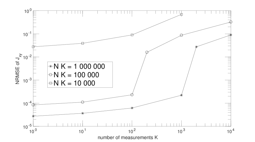
Figure 1: Normalized Root Mean Square Error (NRMSE) of estimation of parameter $J_{xy}$ vs. number $K$ of preparations of each of the $N$ used states.

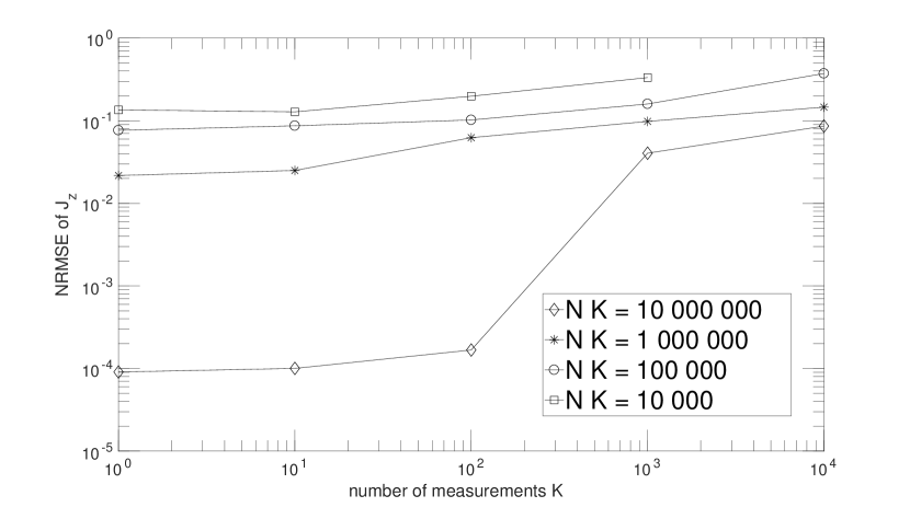
Figure 2: NRMSE of estimation of parameter $J_{z}$ vs. number $K$ of preparations of each of the $N$ used states.

IV.3 Channel estimation and phase estimation

In Sections I and II, we explained that, in the classical framework, the same information processing task is given different names, depending on the considered application field. In particular, the system identification task in the field of automatic control corresponds to the channel estimation task in the field of communications. The same phenomenon occurs in the quantum framework. In particular, QPT, and hence our blind (and possibly single-preparation) extension addressed in Section IV.1, is often stated to be the quantum counterpart of classical system identification (see e.g. [14] p. 389). QPT applies to general quantum systems, not necessarily defined by a small set of parameters, and could therefore be called nonparametric system identification. But the Hamiltonian parameter estimation task, and hence our blind (and single-preparation) extension introduced in Section IV.2, is also closely connected with system identification, and more precisely to parametric system identification, since it estimates a small set of parameters (e.g., the principal values of the exchange tensor in the case of Heisenberg coupling that was considered above as an example), and these parameters then completely define the behavior of that system, including the resulting process matrix in the associated QPT task.

Moreover, although a different terminology is used for other quantum information processing tasks, some of these tasks actually address the same type of problems as above. This first concerns the quantum channel estimation task: as explained e.g. in [49], a map from the density operator associated with a quantum state to another density operator is often called a quantum channel, as a reference to classical communication scenarios. The identification of such a map may therefore be called quantum channel estimation and is closely linked to the QPT problem that we considered above, possibly in its blind and single-preparation form. Similarly, a standard quantum information processing procedure is phase estimation. In [14] p. 221, it is defined as the estimation of the phase $\Phi$ of an eigenvalue $e^{2\pi i\Phi}$ of a unitary operator. This task is therefore related as follows to both investigations reported in Sections IV.1 and IV.2. First, as explained in Section IV.1, the considered (B)QPT problem essentially consists of estimating the parameters $\exp\left[i\frac{J_{xy}(t-t_{0})}{\hbar}\right]$ and $\exp\left[i\frac{J_{z}(t-t_{0})}{2\hbar}\right]$ and hence the exponential terms of the diagonal representation $D$ of the considered operator (see (65)-(LABEL:eq-omega-zero-zero-express)). This is therefore equivalent to estimating the phases of these exponentials, up to a multiple of $2\pi$. Moreover, the method introduced in Section IV.2 is directly connected with removing the additive indeterminacy due to this multiple of $2\pi$.

This discussion shows that the blind and single-preparation extensions that we proposed above in this paper for quantum information processing tasks related to system identification are expected to be of importance not only for the scientific communities focused on QPT and Hamiltonian parameter estimation but also for quantum scientists who investigate a variety of related problems, such as quantum channel estimation and phase estimation. Moreover, in this Section IV, we restricted ourselves to problems related to the characterization (i.e. identification) of the considered quantum process itself. As explained in Sections I and II, related QIP problems consist of building processing systems, with quantum and/or classical means, that essentially implement the inverse of an initially unknown quantum process. This corresponds to the quantum source separation and related tasks, that we investigate in the next section, still aiming at extending the considered configurations to blind and single-preparation ones.

V QIP tasks related to system inversion and state restoration

V.1 Blind quantum source separation

A rather general version of the blind quantum source separation (BQSS) problem addressed here may be defined as follows. A set of qubits with indices $j$ are independently prepared with states $|\psi_{j}\rangle$. The state $|\psi\rangle$ of the system composed of these qubits, which is equal to the tensor product of the above single-qubit states $|\psi_{j}\rangle$, is then transformed, i.e. mapped to another state $|\psi^{\prime}\rangle={\cal M}(|\psi\rangle)$, where the mapping function ${\cal M}$ e.g. corresponds to temporal evolution with coupling between qubits, as detailed below. In the blind configuration, the user is given a set of transformed states $|\psi^{\prime}\rangle$ but does not know the corresponding set of original states $|\psi\rangle$, and hence the source states $|\psi_{j}\rangle$, nor the mapping function ${\cal M}$. The user then eventually wants to restore the information contained in (at least part of) the source states, either in quantum form, by deriving estimates of these states $|\psi_{j}\rangle$, or in classical form, typically by eventually using a classical computer to derive estimates of the coefficients of the states $|\psi_{j}\rangle$ in a given basis.

This generic problem is connected with various application fields. The first one, on which we focus hereafter, is related to the operation of quamputers. In such a future quamputer, data will be stored in registers of qubits, for subsequent use. Due to non-idealities of the physical implementation of such a register, the qubits which form it may have undesired coupling with one another, such as Heisenberg coupling, e.g. if considering quamputer implementations related to spintronics [79, 80, 81]. As time goes on, the register state will therefore evolve in a complicated way due to this undesired qubit coupling, thus making the final value of that register state not directly usable in the target quantum algorithm executed on that quamputer. BQSS may then be used as a preprocessing stage, to restore the initial register state, before providing it to the target application of that quamputer.

To analyze this BQSS problem in more detail, we hereafter focus on a basic case, from which the reader may then extend this analysis to other configurations. In the considered case, the device (e.g., the qubit register) is restricted to two qubits, implemented as electron spins 1/2, and the undesired coupling which exists between them is again based on the cylindrical-symmetry Heisenberg model defined in Appendix C. Using the notations of that appendix, the initial state $|\psi(t_{0})\rangle$ of the device (e.g., the state stored at time $t_{0}$ in the register), which corresponds to state $|\psi\rangle$ in the above general definition of BQSS, may be represented by the column vector $C_{+}(t_{0})$ of the components of $|\psi(t_{0})\rangle$ in the standard basis, defined by (64). Similarly, the final state $|\psi(t)\rangle$ of the device (e.g., the only state available to the user, at a later time $t$, in the register), which corresponds to state $|\psi^{\prime}\rangle$ in the above general definition of BQSS, may be represented by the column vector $C_{+}(t)$ of the components of $|\psi(t)\rangle$ in the standard basis. The effect of coupling is then represented by the relationship

$$C_{+}(t)=MC_{+}(t_{0})$$ (29)

where $M$ is the matrix defined in Appendix C.

The first class of BQSS methods that we previously developed for handling this configuration (see especially [37, 38, 39]) is the “least quantum” one, in the sense that, starting from the available quantum states $|\psi(t)\rangle$, it first converts them into classical-form data (probability estimates) by means of measurements and then processes the latter data with only classical means, as shown in Fig. 3. More precisely, in the reported investigations, only measurements of the components of the two spins along the $Oz$ axis were considered. The probabilities of the outcomes of these measurements are therefore again defined by (12)-(14). Unlike the BQPT method of Section IV.1, the BQSS methods summarized here do not use the SIPQIP framework. Instead, they separately derive an estimate of each set of probabilities $p_{kzz}$, with $k=1$, 2 and 4, associated with one final state $|\psi(t)\rangle$, so that they require each initial state $|\psi(t_{0})\rangle$ to be prepared many times.

Figure 3: Global (i.e. mixing + separating) blind quantum source separation (BQSS) configuration when only applying measurements and classical processing to the available coupled quantum state.

This class of BQSS methods therefore uses the mapping (29), from a state $|\psi(t_{0})\rangle$ to a state $|\psi(t)\rangle$, indirectly: it only involves the mapping (12)-(14), which goes from the set of initial qubit parameters $\{{r}_{1},{r}_{2},\Delta_{I}\}$, to the set of probabilities $\{p_{1zz},p_{2zz},p_{4zz}\}$. The transform (12)-(14) is then the “mixing model”, using the classical BSS terminology and, indeed, even if they are derived from an intrinsically quantum phenomenon, the inputs and outputs of this transform may be stored in classical form, on a classical computer: the moduli ${r}_{j}$ and the phases ${\theta}_{j}$ and ${\phi}_{j}$ (in fact, only their differences ${\phi}_{j}-{\theta}_{j}$ have a physical meaning) may be stored on a classical computer before they are used by the procedure that prepares the corresponding state $|\psi(t_{0})\rangle$. The output of this “mixing stage”, equal to an estimate of $\{p_{1zz},p_{2zz},p_{4zz}\}$, is then connected to the input of the “separating stage” (see Fig. 3 again), which is composed of the separating system that we proposed for restoring an estimate of $\{{r}_{1},{r}_{2},\Delta_{I}\}$ from its input. In other words, this separating system ideally aims at implementing the inverse of the mapping (12)-(14). This can be done (up to an approximation due to estimating the probabilities $p_{kzz}$) in the ideal case when the exact value of the parameter $v$ of (13) is known, because the inverse of (12)-(14) can be analytically determined: see details in [37, 38, 39]. In contrast, the blind version of the problem, i.e. when the value of $v$ is unknown, is handled as follows. One considers the class of direct mappings obtained by replacing $v$ by a free parameter $\overline{v}$ in (12)-(14). One then determines the analytical expression of the corresponding class of inverse mappings, which is derived by replacing $v$ by $\overline{v}$ in the above ideal inverse mapping. The idea is then to derive an estimate $\widehat{v}$ of $v$, in order to use it as the value of $\overline{v}$ in the inverse mapping. Various methods have been proposed to this end (see e.g. [37, 38, 39]), by extending differents concepts used in classical Independent Component Analysis (ICA) to the considered quantum problem.

The complete operation of the above class of BQSS methods consists of two phases, which correspond to the general features that we provided in Section II for classical and quantum machine learning methods:

1. First, in the adaptation (or training) phase, a set of states $|\psi(t)\rangle$ is used to derive the above estimate $\widehat{v}$, i.e. to learn the (direct and) inverse mapping.

2. Then, in the inversion phase (which corresponds to the final, useful, operation of the separating system), the probabilities estimated for each new state $|\psi(t)\rangle$ are transferred through the above estimated inverse mapping, to restore the considered parameters of the corresponding state $|\psi(t_{0})\rangle$.

As mentioned above, a major constraint in that first class of BQSS methods is that it requires the same state $|\psi(t_{0})\rangle$ to be prepared many times, both in the adaptation and inversion phases. This makes these methods “less blind” because, although these states $|\psi(t_{0})\rangle$ are allowed to be unknown from the point of view of the adaptation procedure, some control is required so that the same value is repeatedly prepared for each of these states.

A solution to the above problem was introduced, but only for the inversion phase, in our second class of BQSS methods, especially described in [40, 41, 42]. We now detail it, since we take advantage of it in the fully SIPQIP methods that we introduce further in this paper for BQSS. In that second class of BQSS methods, during the inversion phase, each state $|\psi(t)\rangle$ available as the input of the separating system is directly used in quantum form, i.e. without performing measurements, so that this separating system outputs a quantum state $|\Phi\rangle$ that should ideally be equal to the multi-qubit source state $|\psi(t_{0})\rangle$ that one aims at restoring. That part of the separating system, called the inverting block, is thus a global quantum gate (see Fig. 4), which only requires a single instance of its input state $|\psi(t)\rangle$ to derive its corresponding output state $|\Phi\rangle$.

Figure 4: Mixing stage + quantum-processing inverting block of separating system.

The above gate is designed as follows. Although we here do not keep all the features of the above first class of BQSS methods, we build upon some of its principles. In particular, we exploit the fact that, although the actual value of the mixing matrix $M$ of (29) is not known in the blind configuration, from Appendix C one knows that it belongs to the class of matrices defined as

$$M=QDQ$$ (30)

where $Q=Q^{-1}$ is a known, fixed, matrix and $D$ is a diagonal matrix, whose diagonal entries have unit modulus (and a structure that is disregarded in this approach). We therefore use an inverting block of the separating system which is adaptive (or tunable), i.e. such that some of the values of the parameters that define its behavior may be modified. More precisely, this block is designed so that it is able to implement the inverse of any transform in the above-defined class, depending on its parameter values. Its operation is therefore represented by a matrix defined as

$$U=Q\tilde{D}Q$$ (31)

with

$$\tilde{D} =\left[\begin{tabular}[]{llll}$e^{i\gamma_{1}}$&0&0&0\\ 0&$e^{i\gamma_{2}}$&0&0\\ 0&0&$e^{i\gamma_{3}}$&0\\ 0&0&0&$e^{i\gamma_{4}}$\end{tabular}\right]$$ (36)

where $\gamma_{1}$ to $\gamma_{4}$ are free real-valued parameters. This inverting block is thus the cascade of three simpler quantum gates, as shown in Fig. 4. The implementation of each gate corresponding to the matrix $Q$, as a combination of even simpler gates, was detailed in [38]. Moreover, the adaptive gate corresponding to (36), introduced in [42], may be decomposed as shown in Fig. 5, where the closed (i.e. black) and open circle notations respectively indicate conditioning on the qubit being set to one or zero, as in [14] p. 184. In [42] and in the new use of that gate introduced further in this paper, the values of the parameters $\gamma_{1}$ to $\gamma_{4}$ are controlled by classical-form signals. These parameters may e.g. be independent, known but arbitrary, increasing, functions of control voltages. Such control voltages are e.g. used in the real device described in [81].

Figure 5: Implementation of quantum operator defined by matrix $\tilde{D}$, used in inverting block.

The complete operation of this second class of BQSS methods therefore consists of the same phases as for the above first class of methods:

1. First, in the adaptation phase, a set of states $|\psi(t)\rangle$ is used to adapt the matrix $\tilde{D}$, i.e. to learn the inverse mapping.

2. Then, in the inversion phase, each new state $|\psi(t)\rangle$ is transferred through the gates of Fig. 4, which perform the above estimated inverse mapping, to restore the corresponding state $|\psi(t_{0})\rangle$.

The method used in [42] to adapt the matrix $\tilde{D}$ is based on the probabilities of measurements associated with a set of output states $|\Phi\rangle$ of the inverting block of Fig. 4. These probabilities are essentially used to measure the degree of entanglement of these states $|\Phi\rangle$. The matrix $\tilde{D}$ is adapted so as to essentially make these states $|\Phi\rangle$ unentangled, so that this type of methods performs an “Unentangled Component Analysis” [42], as opposed to the above-mentioned classical and quantum Principal Component Analysis and Independent Component Analysis. The complete structure of the resulting separating system is shown in Fig. 6. Unlike in the inversion phase, during the adaptation phase this structure requires many copies of each of its input states $|\psi(t)\rangle$, in order to derive the corresponding copies of the output states $|\Phi\rangle$ and hence the corresponding probability estimates based on sample frequencies of measurement outcomes. This second class of BQSS methods is thus “more quantum” than the first one, first because it uses quantum processing means in the inverting block, and second because it is based on the quantum concept of entanglement, which has no classical counterpart.

Figure 6: Global (i.e. mixing + separating) configuration, which a feedback separating system that includes a quantum-processing inverting block and a classical-processing adapting block. Each quantum state $|\Phi\rangle$ is used only once (no cloning): see [42].

In the present paper, we introduce a third class of BQSS methods, which proceeds further than the above two classes, by using the SIPQIP framework in all the operation of the separating system, i.e. by using a single preparation of each state also during the adaptation phase. To this end, we exploit the structure of the matrix $D$, defined in (72)-(LABEL:eq-omega-zero-zero-express). We take into account the fact that the matrix $\tilde{D}$ of the separating system should ideally be set to the inverse of $D$. Therefore, by replacing $J_{xy}$ and $J_{z}$ by their estimates $\widehat{J}_{xy}$ and $\widehat{J}_{z}$ in (72)-(LABEL:eq-omega-zero-zero-express), we set $\tilde{D}$ as in (36), but here with the following structure for the phases of its diagonal elements:

$$\gamma_{1}=\frac{GB\tau_{3}}{\hbar}-\frac{\widehat{J}_{z}\tau_{3}}{2\hbar}, \gamma_{2}=-\frac{\widehat{J}_{xy}\tau_{3}}{\hbar}+\frac{\widehat{J}_{z}\tau_{3}}{2\hbar},$$ (37)

$$\gamma_{3}=\frac{\widehat{J}_{xy}\tau_{3}}{\hbar}+\frac{\widehat{J}_{z}\tau_{3}}{2\hbar}, \gamma_{4}=-\frac{GB\tau_{3}}{\hbar}-\frac{\widehat{J}_{z}\tau_{3}}{2\hbar}$$ (38)

where $\tau_{3}$ is the value of the time interval $(t-t_{0})$ used in the inversion phase of the proposed BQSS method. In this new BQSS method, we take advantage of the BQPT method that we described in Section IV.1: when applying the latter method with time intervals $(t-t_{0})$ set according to (11) with a freely selected value of $\tau_{1}$, we get (21) and (23), which shows that all the quantities in (37)-(38) required to assign $\gamma_{1}$ to $\gamma_{4}$ are known or can be estimated. The adaptation phase of the proposed BQSS method therefore consists of applying the above BQPT method, then using (37)-(38) to derive the selected values of $\gamma_{1}$ to $\gamma_{4}$ and finally using the supposedly known correspondence function which makes it possible to convert these values of $\gamma_{1}$ to $\gamma_{4}$ into the practical control signals (e.g., voltages) of the gates of Fig. 5 which make these gates operate with these desired values of $\gamma_{1}$ to $\gamma_{4}$. The resulting global configuration is shown in Fig. 7. Each state $|\psi(t)\rangle$ is thus used only once (see also [42] about the no-cloning theorem): during the adaptation phase, these states are sent to the part of the system which performs measurements and BQPT (dashed line and lower part of Fig. 7); then, during the inversion phase, they are sent to the inverting block (dash-dotted line and upper right part of Fig. 7).

Figure 7: Global (i.e. mixing + separating) configuration, with a feedforward separating system that includes a quantum-processing inverting block and a classical-processing adapting block. Each quantum state $|\psi(t)\rangle$ is used only once (no cloning): see text.

Thanks to the properties of the BQPT method reused here as a building block of the proposed BQSS method, the output of the latter method does not depend on the values used in (21) and (23) for the integers $\widehat{k}_{xy}$ and $\widehat{k}_{z}$. This may be seen by inserting (21)-(23) in (37)-(38) and then in (36), with (11), which shows that the terms of (21)-(23) that include $\widehat{k}_{xy}$ and $\widehat{k}_{z}$ yield terms in (37)-(38) that are integer multiples of $2\pi$, and that therefore have no influence on the value of $\tilde{D}$.

V.2 Blind quantum (entangled) state restoration

In the classical framework, the concept of blind source separation (BSS) intrinsically refers to situations involving several (unknown) source signals, created by several “sources” that may be some kinds of “objects”. Such a situation may be mathematically described by gathering all the values of these source signals, e.g. at a given time, as the elements of an overall source vector. In our quantum extensions of this classical BSS, we started from a similar situation, involving several objects, such as qubits implemented as spins 1/2, and we first independently considered the “signal value”, i.e. the initial quantum state $|\psi_{j}(t_{0})\rangle$, of each of them (see (58)). We then “gathered” these individual states by defining the state of the complete system (see (62)) as the tensor product of the states $|\psi_{j}(t_{0})\rangle$, somehow as the quantum counterpart of the above vector of classical signal values. However, the quantum framework opens the way to much richer situations, because the possible states of a complete system are not restricted to the tensor products of the individual states of independent parts of this system: they also include entangled states. An extension of the above BQSS problem is therefore blind quantum state restoration (BQSR), aiming at restoring a possibly entangled deterministic pure state of a multi-qubit system, starting from an altered version of it. One thus conceptually considers a single arbitrary multi-qubit source state, instead of several single-qubit source states. In particular, this includes restoring the possibly entangled initial state $|\psi(t_{0})\rangle$ of a multi-qubit system, from the state $|\psi(t)\rangle$ of that system at a later time.

We here investigate this extension of BQSS to possibly entangled source states, by considering the use of such states in the second phase of the operation of this system, i.e. in the above-defined inversion phase, after the transform performed by this system has been fixed by means of the adaptation phase. We claim that the BQSS system defined in Fig. 7 is directly able to perform the considered BQSR task, since it operates as follows. An unknown state $|\psi(t_{0})\rangle$ is created, then modified by an operator represented by the matrix $M$, thus yielding the state $|\psi(t)\rangle$. The latter state is the state processed by the new separating system that we designed in Section V.1. The transform performed by this system is represented by the matrix $U=Q\tilde{D}Q$ (see (31)). But, during the adaptation phase of that separating system that occurred before this inversion phase, $U$ was made equal to the inverse of $M$ (up to estimation errors) by the proposed adaptation method. Therefore, when applying that separating transform $U$ to $|\psi(t)\rangle$, the output state of the separating system becomes equal to $|\psi(t_{0})\rangle$ (up to estimation errors) and this analysis does not depend at all whether $|\psi(t_{0})\rangle$ is entangled or not. In particular, if the proposed BQSS (and hence BQSR) method is used to restore the initial state of a qubit register by compensating for the undesired coupling between its qubits, as discussed above, this means that this method also applies when an entangled state is stored in this qubit register.

V.3 Blind quantum channel equalization

As discussed in Sections I, II and IV.3, in the classical and quantum frameworks, the same information processing task is given different names depending on the considered application field. This is also true for the generic QIP problem, related to system inversion, that we initially defined for non-entangled states at the beginning of Section V.1 , that we then extended to possibly entangled states in Section V.2 and that may be summarized as follows: a user is given a set of transformed states $|\psi^{\prime}\rangle={\cal M}(|\psi\rangle)$, but does not know the original states $|\psi\rangle$, nor the mapping function ${\cal M}$; the user wants to restore the original states $|\psi\rangle$. Whereas we illustrated that QIP task with one type of application in Sections V.1 and V.2, we anticipate that it will have various other applications as the quite general field of QIP keeps on growing. In particular, this problem too may be rephrased as a quantum communication scenario. The above user is then the receiver, who only knows the received states $|\psi^{\prime}\rangle$, that have been altered by the channel ${\cal M}$. Without knowing that channel, the receiver aims at restoring the emitted states $|\psi\rangle$ that he does not know either (or the information, in classical form, contained in these states $|\psi\rangle$). This therefore corresponds to the blind quantum channel equalization problem and the generic methods that we proposed in Sections V.1 and V.2 also allow one to solve this problem, moreover with the advantages of the proposed SIPQIP framework.

VI Contributing to quantum classification

We now come back to the other main aspect of machine learning discussed in Section II, namely classification. In the classical framework, many classification algorithms receive data that consist of vectors which contain features that characterize the “objects” to be classified [67]. These algorithms heavily rely on computing the dot (i.e., scalar or inner) product $v_{j}^{T}v_{k}$ of two column vectors $v_{j}$ and $v_{k}$, where ^T stands for transpose, or on computing the distance $||v_{j}-v_{k}||$ between the associated two data points [67]. These two quantities are moreover directly connected, since

$$||v_{j}-v_{k}||^{2}=||v_{j}||^{2}+||v_{k}||^{2}-2v_{j}^{T}v_{k}.$$ (39)

In particular, for any unit-norm vectors, this yields

$$||v_{j}-v_{k}||^{2}=2(1-v_{j}^{T}v_{k}).$$ (40)

Using the signal/data processing terminology, $v_{j}^{T}v_{k}$ is also the basic, i.e. non-centered and non-normalized, correlation parameter of the data vectors $v_{j}$ and $v_{k}$, whereas their non-centered correlation coefficient (also called the cosine similarity [67]) is

$$\rho(v_{j},v_{k})=\frac{v_{j}^{T}v_{k}}{||v_{j}||.||v_{k}||}.$$ (41)

These two correlation parameters coincide for unit-norm vectors. The correlation coefficient $\rho(v_{j},v_{k})$ is e.g. widely used for data characterization and classification by the Earth observation (i.e. remote sensing) community. Each of the vectors $v_{j}$ and $v_{k}$ then typically defines a spectrum, which consists of the light reflectance values of a material at a set of “frequencies” (in fact, narrow spectral bands) [31]. More precisely, one then computes the arccosine of $\rho(v_{j},v_{k})$, which is equal to the angle between $v_{j}$ and $v_{k}$ [67] and is therefore called the “Spectral Angle Mapper” (SAM) between these vectors [82]. A low value of that SAM corresponds to a high value of the “spectral similarity” of the considered materials, i.e. of their similarity in terms of the shape of the variations of their reflectance functions with respect to frequency (where “shape” means regardless of their global scale: that scale has no influence on (41) and hence on SAM). Similar approaches are used in the field of Astrophysics, with spectral data vectors which consist of luminance values (i.e. direct light flux from the observed object), instead of reflectance.

Let us now consider the situation when data that are initially in classical form are to be classified by using a quantum classifier, in order to achieve higher classification speed [83, 10, 67]. This first requires one to transform the initial classical data into quantum states. To this end, each classical-form vector is stored in a qubit register with index $r$, that consists of $Q$ qubits. Each individual qubit is thus indexed by $r$ and $q\in\{1,\dots,Q\}$. Its state space is denoted as ${\cal E}_{rq}$ and a basis of this space is composed of the two kets $|k_{rq}\rangle_{rq}$ with $k_{rq}\in\{0,1\}$. All deterministic pure states of the qubit register $r$ then belong to the space ${\cal E}_{r1}\otimes\dots{\cal E}_{rQ}$ and read

$$|\psi_{r}\rangle=\sum_{{\cal S}(k_{r\bullet})}c_{rk_{r1}\dots k_{rQ}}|k_{r1}\rangle_{r1}\otimes\dots\otimes|k_{rQ}\rangle_{rQ}$$ (42)

where the compact notation ${\cal S}(k_{r\bullet})$ means: the set of all values of the ordered set of $Q$ integers $k_{rq}$ corresponding to the fixed value $r$ and to all values $q\in\{1,\dots,Q\}$, again with $k_{rq}\in\{0,1\}$. Besides, the $2^{Q}$ complex-valued coefficients $c_{rk_{r1}\dots k_{rQ}}$ are indexed by the index $r$ of the considered register and by all integers $k_{rq}$ which define to which basis state each coefficient $c_{rk_{r1}\dots k_{rQ}}$ corresponds. These coefficients are such that $|\psi_{r}\rangle$ has unit norm. Let us then consider a classical-form complex-valued unit-norm vector $v_{j}$ with dimension $2^{Q}$ (or lower: zero-valued components are then added to $v_{j}$ to reach $2^{Q}$ components). This vector may be stored in a ket $|\psi_{r}\rangle$ defined by (42), by setting the coefficients $c_{rk_{r1}\dots k_{rQ}}$ of $|\psi_{r}\rangle$ respectively to the values of the components of $v_{j}$ (a common phase reference may be used for all considered kets). If the norm of $v_{j}$ is not equal to one, it may be handled separately, while $v_{j}/||v_{j}||$ is stored in $|\psi_{r}\rangle$, as stated in [83].

The above-defined kets (42) may then be employed in quantum classifiers, which often use (i) the dot product $\langle\psi_{1}|\psi_{2}\rangle$ of such kets or (ii) the squared modulus of this dot product, which is called the overlap of these kets (see [84, 85] or [67] p. 120), or (iii) the distance between the points associated with such kets, as e.g. discussed in [83, 10, 67]. The dot product formally associated with two states (42) respectively stored in registers with indices $r=1$ and $r=2$ is defined as if these kets belonged to the same state space. This dot product therefore reads

$$\langle\psi_{1}|\psi_{2}\rangle=\sum_{{\cal S}(k_{r\bullet})}c_{1k_{r1}\dots k_{rQ}}^{*}c_{2k_{r1}\dots k_{rQ}}$$ (43)

where ^∗ stands for complex conjugate. Some quantum circuits were proposed in the literature for computing the corresponding state overlap. A widely used approach, called the swap test, was proposed in [86] to essentially test the equality of two states. The quantity used to this end is the probability of an outcome of a measurement performed at the output of the considered circuit. This quantity is equal to 0 if the considered states are equal, and essentially equal to 1/2 otherwise (more precisely, it is higher than a bound close to 1/2 if the states are far enough from one another). Beyond this binary decision, this probability is a continuous-valued quantity, which may be shown to be linearly related to the overlap of the considered quantum states (part of the corresponding calculations are provided in [86, 67]). Another approach for computing the overlap of quantum states is based on the circuit of Fig. 6(B) of [84]. The behavior of that circuit is only briefly defined in [84], which outlines how to express the overlap associated with the density operators of the two multi-qubit inputs of the considered circuit as the result of classical post-processing applied to the results of measurements performed at the output of that circuit. Our own calculations (to be detailed elsewhere), performed for deterministic pure input states $|\psi_{1}\rangle$ and $|\psi_{2}\rangle$, confirm that the squared modulus of (43) may be expressed as a (multistage) linear combination of probabilities of outcomes of measurements performed at the output of that quantum circuit. In appendix F, we show how the above quantum circuits may be further exploited in order to compute dot products $\langle\psi_{1}|\psi_{2}\rangle$, not only their (squared) moduli.

The above dot products or overlaps may be used in various ways in the general framework of quantum classification. More specifically, we hereafter show how enhanced approaches may be developed by combining quantum classification principles that use dot products or overlaps with our SIPQIP, i.e. single-preparation, concept. We illustrate this approach with a first original contribution to single-preparation quantum classification, that will be extended in future papers. In this contribution, we focus on the second phase of the operation of a classifier, that is on the “resolution phase” defined in Section II, which takes place after the (unsupervised or supervised) learning phase. This is, by the way, similar to what we did for BQSS, by first applying our SIPQIP concept to the second phase of operation, i.e. the inversion phase, before we extended it to the first, i.e. adaptation, phase as explained in Section V.1.

In the proposed approach, we consider the situation when the classical-form vectors to be classified are characterized by their shapes, not their magnitudes, e.g. as in the Earth observation and Astrophysics applications outlined at the beginning of the present section. Therefore, these vectors may initially be rescaled to have unit norm, so that this norm is not an issue when transforming these classical vectors into quantum states. We hereafter address the general situation when the considered classification problem involves $C$ classes, indexed by $c$, with $c\in\{1,\dots,C\}$. Moreover, we consider the usual case when the classical-form data vectors, and hence the associated dot products of kets, are real-valued.

To describe how classification is here performed, let us first consider the non-realistic situation when each class with index $c$ is initially defined by a single known classical-form vector $v_{c1}$ and hence a single associated quantum state $|\psi_{c1}\rangle$. When analyzing a new “object” of the considered application (e.g. the spectrum of an unknown material in the above Earth observation or Astrophysics applications), represented by a quantum state $|\phi\rangle$, a basic method for classifying that object consists of separately estimating its dot product $\langle\phi|\psi_{c1}\rangle$ with each of the states $|\psi_{c1}\rangle$ and in deciding that this object belongs to the class which yields the highest estimated value of the dot product $\langle\phi|\psi_{c1}\rangle$, i.e. the best similarity with $|\phi\rangle$. This approach may be simplified as follows in the case when the components of the considered classical-form data vectors are nonnegative, which e.g. applies to the reflectance or luminance values that compose the above-mentioned spectra. In that case, the square root of the overlap $|\langle\phi|\psi_{c1}\rangle|^{2}$ coincides with the corresponding dot product $\langle\phi|\psi_{c1}\rangle$. This overlap is therefore sufficient for measuring similarity in that case (as opposed to the sign indeterminacy that it yields with respect to the dot product for possibly negative data). The above classifier then operates equivalently by deciding that the considered object belongs to the class which yields the highest estimated value of overlap $|\langle\phi|\psi_{c1}\rangle|^{2}$. This is attractive, because an overlap is computed more easily that the corresponding dot product, as shown in Appendix F.

An improved variant of the above classification method employs a user-defined threshold in addition, in order to achieve the rejection capability defined in Section II: if the highest of the above dot products (or overlaps, in the simplified version) remains lower than this threshold, the considered object is “rejected”, i.e. the classifier decides that it is not able to classify that object, because it is not similar enough to any of the classes of objects that are known in the considered problem.

All these classifiers are based on computing overlaps, because their decisions are either directly based on such overlaps or based on dot products, that may be derived from overlaps, as explained in Appendix F. Each of these overlaps, such as $|\langle\phi|\psi_{c1}\rangle|^{2}$, is typically estimated by using the sample frequency estimate(s) of one or several types of probabilities associated with overlap in the quantum circuits that were defined above for estimating overlaps. This then means that, for each class $c$, many copies (typically $10^{5}$, as explained in Section III.1) of the state $|\psi_{c1}\rangle$ must be prepared to estimate these probabilities.

Now consider the realistic version of the above problem, when each class with index $c$ is initially defined by a full set of classical-form vectors $v_{cj}$, with a vector index $j$ ranging from 1 to a maximum value that may depend on the class. These vectors are then transformed into quantum states $|\psi_{cj}\rangle$. The above classifiers may be extended as follows for this situation, focusing on their version that directly bases its decisions on overlaps, for the sake of clarity. For each class, one may first compute a full set of (estimates of) overlaps $|\langle\phi|\psi_{cj}\rangle|^{2}$ and these quantities should then be reduced to a single parameter that characterizes the overall similarity of the considered class with $|\phi\rangle$. A natural parameter that may be used to this end is the mean of all overlaps $|\langle\phi|\psi_{cj}\rangle|^{2}$ associated with the considered class. Here again, in practice, only an estimate of this mean overlap is obtained, by using various quantum state preparations and measurements. However, unlike in the above non-realistic scenario, this may here be achieved with two quite different approaches. The first approach, which might be considered as the most natural one if disregarding our previous contributions in this paper, consists of separately estimating each of the overlaps $|\langle\phi|\psi_{cj}\rangle|^{2}$ as above, therefore typically preparing $10^{5}$ copies of each state $|\psi_{cj}\rangle$ (and of $|\phi\rangle$), and then computing (on a classical computer) the mean of these estimated overlaps. This is an application of the standard, multiple-preparation, approach defined in Section III.1. However, we stress that we here only aim at computing the mean of this finite set of overlaps, so that we only need to estimate the mean(s) of the corresponding set(s) of probabilities (as explained above, this involves one or several types of probabilities, depending on the considered quantum circuit). In Section III.3, we showed that this may be performed much more efficiently by using our SIPQIP framework, which here means decreasing the number of preparations per state $|\psi_{cj}\rangle$ and taking advantage of the averaging of measurement results that is then performed over all these states (thus still requesting one copy of $|\phi\rangle$ per measurement). This number of preparations per state may even be decreased down to one if enough different states $|\psi_{cj}\rangle$ are available to reach a high enough estimation accuracy: in [26] and Section IV.2.2 of the present paper, we analyzed the numerical performance achieved by this SIPQIP approach for the BQPT and BHPE tasks, and we plan to investigate it for classification in future papers. In the literature, quantum classifiers have especially been considered for big-data, i.e. large-scale, applications [10, 83]. In such applications, the above-mentioned large number of states $|\psi_{cj}\rangle$ will actually be available and our SIPQIP framework will take full advantage of it (besides, it can also attractively operate with a somewhat lower total number of states $|\psi_{cj}\rangle$ and a number of preparations per state somewhat higher than one).

VII Conclusion

The term “machine learning” especially refers to algorithms (and associated systems) that derive mappings, i.e. intput/output transforms, by using numerical data that provide information about the transform which is of interest in the considered application. The data processing tasks to be performed in these applications not only include classification and regression, but also system identification, system inversion and input signal restoration (or source separation when considering several signals). Whereas these problems have been and are still widely investigated in a purely classical framework, part of them are currently being extended to configurations which involve quantum-form data and/or quantum processing means. Within this general quantum framework, we here tackled the most challenging configurations from two points of view. First, almost all this paper is devoted to unsupervised, i.e. blind, configurations, which have not been addressed in the literature for most of the tasks considered here. Unsupervised learning is very attractive because, as detailed in Sections I and II, it avoids the need for known “reference values” (e.g., input values for system identification) to learn the required mappings. Second, we here mainly aim at extending a variety of aspects of quantum machine learning by introducing new algorithms which can operate with only one instance of each prepared state (where the term “preparation” is used for both deterministic and random pure states, as explained in Section I). This approach first avoids the burden of having to prepare many ideally identical copies of each used state in order to compute statistical parameters separately for each such state. Moreover, this approach yields much better performance than the multiple-preparation approach for a given total number of state preparations, as shown for blind quantum process tomography in our very recent paper [26] and confirmed here by our new results for blind Hamiltonian parameter estimation. Besides, this original single-preparation approach is especially of interest when combined with unsupervised learning, because using the multiple-preparation approach instead, in the unsupervised framework, would mean allowing the “reference values” to be unknown but still requesting that the same (unknown) reference value be prepared many times, which would still require significant control in the considered quantum learning procedure, so that this procedure would be “less unsupervised”.

The above concepts thus result in a general SIngle-Preparation Quantum Information Processing (SIPQIP) framework. We illustrated it for various processing tasks, including with a quantitative evaluation of the numerical performance that it yields. For the tasks related to the blind, i.e. unsupervised, version of system identification (including quantum process tomography and Hamiltonian parameter estimation), system inversion and signal restoration (including source separation), we showed how to apply the proposed approach to a concrete example, related to spintronics, which involves Heisenberg coupling between two qubits. Starting from the explicit algorithms and system architectures that we detailed for this configuration, the reader may then adapt them to other types of processes, and we will also extend this approach to other processes in the future. Similarly, we provided a first illustration of the application of this SIPQIP framework to quantum classification and we plan to report extensions of this approach in future papers.

Moreover, when aiming at compensating for undesired Heisenberg coupling between qubits, we proposed two quantum system architectures: see Fig. 6 for a feedback structure and Fig. 7 for a feedforward structure. These architectures open the way to the much more general concept of “self-adaptive quantum gates”, i.e. gates which include the following two features:

1. some means for controlling the values of parameters that define the quantum state transform that such a gate performs within a predefined class of transforms,

2. an autonomous (i.e. blind or unsupervised) algorithm which controls the adaptation of these parameter values, so as to achieve a predefined condition, that could consist of ensuring output disentanglement, as in the above example, or that could be a counterpart of that condition, depending on the available data and on the type of undesired behavior that one wants to compensate for.

Such gates would especially be of interest for a quantum computer that, by the way, we proposed to more briefly call a “quamputer”: by adequately selecting the above-mentioned adaptation condition and designing an associated adaptation algorithm, one could create a self-adaptive quantum gate that automatically compensates for a given type of non-ideality (instead of undesired Heisenberg coupling in the above example) that occurs e.g. in a gate that precedes the considered self-adaptive gate, thus allowing practical future quamputers to operate correctly despite these non-idealities, thanks to their internal compensation means.

Appendix A Connection of single-preparation and multiple-preparation QIP with classical adaptive processing

Various types of classical data processing methods are based on adapting the parameter values of a system, e.g. of a filter, an artificial neural network (including the above-mentioned deep learning approaches) or a blind source separation system (see e.g. [29, 31, 51, 87, 32, 1, 9, 88, 89] and references in Sections I and II). This adaptation is based on a set of (often multidimensional) data samples, which are typically used to minimize a cost function that depends on the considered problem. This yields the following two approaches.

The first approach corresponds to so-called batch algorithms [32, 9]. These algorithms are often iterative, and each of their steps uses the complete set of available data samples. This especially includes gradient descent algorithms [87] (i.e., steepest descent algorithms [51]), where each step uses the gradient of the cost function defined by all data samples to perform one update for all parameters.

The cost functions of the above algorithms, and hence their gradients, are often defined as the mean of an “elementary term” associated with a single data sample, where this mean is the expectation if considering a probabilistic representation, or the mean (or sum) over all data samples if using an empirical framework. The second type of adaptation algorithms is then derived from the first one essentially by removing the above mean from the update rule used in each adaptation step [51, 87, 89] (see e.g. [9] for comments about Robbins-Monro algorithms and stochastic approximation theory). Each such step thus uses only the “elementary term” associated with a single data sample (or a few samples [1]), where this term corresponds to a random variable in a probabilistic framework (as opposed to the expectation of these terms used in deterministic, batch, algorithms). This yields so-called online [32, 9] or stochastic algorithms, and especially stochastic gradient descent algorithms [51, 1], including the famous least-mean-square (LMS) or Widrow-Hoff algorithm [51, 87, 9, 88, 89].

If only considering a single step of the above second type of algorithms, these algorithms may at first glance appear not to be sound, because such a step only uses the elementary term associated with a single data sample to estimate the relevant expectation derived for the above first type of algorithms. However, one should instead consider the complete set of adaptation steps, which uses (once or repeatedly [9]) all data points: this overall set of steps of the algorithm eventually yields relevant behavior.

Unlike most above classical methods, the procedure that we described in Section III.2 does not concern iterative algorithms for optimizing a cost function. However, these two types of methods share a two-level structure, where the lower level uses only one (or a few) data sample(s), and the higher level gathers all the contributions derived from the lower level, thus extracting overall information that is relevant for the considered applications.

The lower level of these quantum methods might therefore be stated to be “stochastic” (in the sense “using a single data sample”), but that might be misleading for some QIP tasks, so that we instead call them “single-preparation (QIP) methods”, for the sake of clarity. Therefore, the QIP methods based on the approach of Section III.1 are called “multiple-preparation (QIP) methods”, whereas they might have been called “batch (QIP) methods”, as a reference to the above batch classical methods.

Appendix B Validating the single-preparation QIP framework with Kolmogorov’s approach

One may decide to use the approach defined in Section III.2 only as a means for proposing to use the expression obtained in (10) as an estimator of the quantity of interest, that is of $E\{P(A_{k})\}$ for any $k\in\{1,\dots,2^{Q}\}$, and to then validate the relevance of this estimator from scratch, by using Kolmogorov’s view of probabilities (see e.g. [68]). This validation consists of deriving the mean (and hence bias) and variance of this estimator. It is provided hereafter, first for a finite number $L$ of trials, and then for the asymptotic case $L\rightarrow+\infty$.

The result of the trial with index $\ell$, which corresponds to the indicator function in (10), is here represented by a binary-valued random variable denoted as ${\rm X}_{\ell}$, which takes the values 1 and 0 respectively with probabilities $P(A_{k},\ell)$ (defined as in Section III.2) and $[1-P(A_{k},\ell)]$. Then, the overall result (10) for all $L$ trials is represented by the random variable

$$\overline{{\rm X}}=\frac{\sum_{\ell=1}^{L}{\rm X}_{\ell}}{L}$$ (44)

where we omit in notations that all ${\rm X}_{\ell}$ and hence $\overline{{\rm X}}$ depend on $k$.  
 

B.1 Mean of $\overline{{\rm X}}$ for a finite $L$

As a first scenario, let us consider the case when the pure states $|\psi(n)\rangle$ and hence the quantities $P(A_{k},\ell)$ are deterministic and the number $K$ of copies of each state $|\psi(n)\rangle$ is arbitrary (including $K=1$). It is then easily shown that

$$E_{1}\{{\rm X}_{\ell}\}=P(A_{k},\ell)$$ (45)

where $E_{1}\{.\}$ stands for expectation, i.e. statistical averaging with respect to the possible values (1 and 0) of ${\rm X}_{\ell}$, with their above fixed probabilities, in this first scenario. Eq. (44) then yields

$$E_{1}\{\overline{{\rm X}}\}=\frac{\sum_{\ell=1}^{L}P(A_{k},\ell)}{L}.$$ (46)

Then, the second scenario, which is the one of interest here, is when the quantities $P(A_{k},\ell)$ are stochastic and their samples are drawn with the same statistical distribution for all values of $\ell$. The expectation of this distribution is denoted as $E\{P(A_{k})\}$, since it does not depend on $\ell$. The expectation $E_{2}\{\overline{{\rm X}}\}$ of $\overline{{\rm X}}$ is then obtained by performing statistical averaging not only with respect to the possible values of ${\rm X}_{\ell}$, as above, but also with respect to the possible values of the quantities $P(A_{k},\ell)$. Applying the latter averaging to (46) yields

$$E_{2}\{\overline{{\rm X}}\} = \frac{\sum_{\ell=1}^{L}E\{P(A_{k},\ell)\}}{L}$$ (47)

$$= E\{P(A_{k})\}.$$ (48)

So, for a finite $L$, the expectation of the proposed estimator $\overline{{\rm X}}$ of $E\{P(A_{k})\}$ is equal to $E\{P(A_{k})\}$, i.e. this estimator is unbiased.

B.2 Asymptotic mean of $\overline{{\rm X}}$

Starting from the above second scenario, when $L$ tends to infinity, the above mean (48) of course remains equal to $E\{P(A_{k})\}$. The proposed estimator $\overline{{\rm X}}$ of $E\{P(A_{k})\}$ is therefore asymptotically unbiased.

It should be noted that, in the above first scenario, (46) similarly yields

$$\lim_{L\rightarrow+\infty}E_{1}\{\overline{{\rm X}}\}=\lim_{L\rightarrow+\infty}\frac{\sum_{\ell=1}^{L}P(A_{k},\ell)}{L}$$ (49)

provided this limit exists. This result is consistent with the frequentist view of probabilities and statistical mean because, in the latter view, the right-hand term of (49) is the statistical mean of the samples $P(A_{k},\ell)$.

B.3 Variance of $\overline{{\rm X}}$ for a finite $L$

We here consider the case when the number $K$ of copies of each state $|\psi(n)\rangle$ is equal to one, assuming these states are independently drawn (with the same distribution again) in the second scenario. For both scenarios, it may be shown that the random variables ${\rm X}_{\ell}$ are uncorrelated and that the variance of $\overline{{\rm X}}$, defined with $E_{1}\{.\}$ or $E_{2}\{.\}$ depending on the considered scenario, meets

$$\mathrm{var}\{\overline{{\rm X}}\}=\frac{\sum_{\ell=1}^{L}\mathrm{var}\{{\rm X}_{\ell}\}}{L^{2}}.$$ (50)

For deterministic values of the quantities $P(A_{k},\ell)$, the variance of each random variable ${\rm X}_{\ell}$ is easily calculated, and (50) then yields

$$\mathrm{var}_{1}\{\overline{{\rm X}}\}=\frac{\sum_{\ell=1}^{L}[P(A_{k},\ell)-P(A_{k},\ell)^{2}]}{L^{2}}.$$ (51)

Since $P(A_{k},\ell)\in[0,1]$, Eq. (51) yields

$$0\leq\mathrm{var}_{1}\{\overline{{\rm X}}\}\leq\frac{1}{4L}.$$ (52)

For stochastic values of the quantities $P(A_{k},\ell)$, one similarly obtains

$$\mathrm{var}_{2}\{\overline{{\rm X}}\}=\frac{E\{P(A_{k})\}-{(E\{P(A_{k})\})^{2}}}{L}$$ (53)

and

$$0\leq\mathrm{var}_{2}\{\overline{{\rm X}}\}\leq\frac{1}{4L}.$$ (54)

B.4 Asymptotic variance of $\overline{{\rm X}}$

Eq. (52) and (54) directly yield

$$\lim_{L\rightarrow+\infty}\mathrm{var}_{1}\{\overline{{\rm X}}\} = 0$$ (55)

$$\lim_{L\rightarrow+\infty}\mathrm{var}_{2}\{\overline{{\rm X}}\} = 0.$$ (56)

This, together with the above result concerning the asymptotic mean of the proposed estimator $\overline{{\rm X}}$, shows that this estimator is asymptotically efficient. This is the counterpart, for our framework, of the convergence/stability analysis of the non-quantum adaptive systems considered in Appendix A.

Appendix C Considered quantum process and state properties

In this paper, we consider a device composed of two distinguishable [42] qubits implemented as electron spins 1/2, that are internally coupled according to the cylindrical-symmetry Heisenberg model, which is e.g. relevant for spintronics applications [80, 79, 81]. The symmetry axis of this model is here denoted as $Oz$. The considered spins are supposed to be placed in a magnetic field (also oriented along $Oz$ and with a magnitude $B$) and thus coupled to it. Moreover, we assume an isotropic $\overline{\overline{g}}$ tensor, with principal value $g$. The time interval when these spins are considered is supposed to be short enough for their coupling with their environment to be negligible. In these conditions, the temporal evolution of the state of the device composed of these two spins is governed by the following Hamiltonian:

$$H = Gs_{1z}B+Gs_{2z}B-2J_{xy}(s_{1x}s_{2x}+s_{1y}s_{2y})$$ (57)

$$-2J_{z}s_{1z}s_{2z}$$

where:

• $G=g\mu_{e}$, where $\mu_{e}$ is the Bohr magneton, i.e. $\mu_{e}=e\hbar/2m_{e}=0.927\times 10^{-23}JT^{-1}$ and $\hbar$ is the reduced Planck constant,

• $s_{jx},\ s_{jy},\ s_{jz}$, with $j\in\{1,2\},$ are the three components of the vector operator $\overrightarrow{s_{j}}$ associated with spin $j$ in a cartesian frame,

• $J_{xy}$ and $J_{z}$ are the principal values of the exchange tensor.

Among the above parameters, the value of $g$ may be experimentally determined, and $B$ can be measured. The values of $J_{xy}$ and $J_{z}$ are here assumed to be unknown.

We here suppose that each spin $j$, with $j\in\{1,2\},$ is prepared, i.e. initialized, at a given time $t_{0}$, in the pure state

$$|\psi_{j}(t_{0})\rangle=\alpha_{j}|+{\rangle}+\beta_{j}|-{\rangle}$$ (58)

where $|+\rangle$ and $|-\rangle$ are eigenkets of $s_{jz}$, for the eigenvalues $1/2$ and $-1/2$ respectively. We will further use the polar representation of the qubit parameters $\alpha_{j}$ and $\beta_{j}$, which reads

$$\alpha_{j}={r}_{j}e^{i{\theta}_{j}}\hskip 14.22636pt\beta_{j}={q}_{j}e^{i{\phi}_{j}}\hskip 28.45274ptj\in\{1,2\}$$ (59)

where $i$ is the imaginary unit, and with $0\leq{r}_{j}\leq 1$ and

$${q}_{j}=\sqrt{1-{r}_{j}^{2}}\hskip 28.45274ptj\in\{1,2\}$$ (60)

because each spin state $|\psi_{j}(t_{0})\rangle$ has unit norm. Moreover, for each couple of phase parameters ${\theta}_{j}$ and ${\phi}_{j}$, only their difference has a physical meaning. After they have been prepared, these spins are coupled according to the above-defined model for $t\geq t_{0}$.

Hereafter, we consider the state of the overall system composed of these two spins. At time $t_{0}$, this state is equal to the tensor product of the states of both spins defined in (58). It therefore reads

$$|\psi(t_{0})\rangle = |\psi_{1}(t_{0})\rangle\otimes|\psi_{2}(t_{0})\rangle$$ (62)

$$= \alpha_{1}\alpha_{2}|++\rangle+\alpha_{1}\beta_{2}|+-\rangle$$

$$+\beta_{1}\alpha_{2}|-+\rangle+\beta_{1}\beta_{2}|--\rangle$$

in the four-dimensional basis ${\cal B}_{+}=\{|++\rangle,|+-\rangle,|-+\rangle,|--\rangle\}$.

The state of this two-spin system then evolves with time. Its value $|\psi(t)\rangle$ at any subsequent time $t$ may be derived from its above-defined Hamiltonian. It is defined [38] by

$$C_{+}(t)=MC_{+}(t_{0})$$ (63)

where $C_{+}(t_{0})$ and $C_{+}(t)$ are the column vectors of components of $|\psi(t_{0})\rangle$ and $|\psi(t)\rangle$, respectively, in basis ${\cal B}_{+}$. For instance, as shown by (62),

$$C_{+}(t_{0})=[\alpha_{1}\alpha_{2},\alpha_{1}\beta_{2},\beta_{1}\alpha_{2},\beta_{1}\beta_{2}]^{T}$$ (64)

where ^T stands for transpose. Moreover, the matrix $M$ of (63), which defines the transform applied to $|\psi(t_{0})\rangle$, reads

$$M=QDQ^{-1}=QDQ$$ (65)

with

$$Q=Q^{-1}=\left[\begin{tabular}[]{llll}1&0&0&0\\ 0&$\frac{1}{\sqrt{2}}$&$\frac{1}{\sqrt{2}}$&0\\ 0&$\frac{1}{\sqrt{2}}$&$-\frac{1}{\sqrt{2}}$&0\\ 0&0&0&1\end{tabular}\right]$$ (66)

and $D$ equal to

$$\left[\begin{tabular}[]{llll}$e^{-i\omega_{1,1}(t-t_{0})}$&0&0&0\\ 0&$e^{-i\omega_{1,0}(t-t_{0})}$&0&0\\ 0&0&$e^{-i\omega_{0,0}(t-t_{0})}$&0\\ 0&0&0&$e^{-i\omega_{1,-1}(t-t_{0})}$\end{tabular}\right].$$ (71)

(72)

The four real (angular) frequencies $\omega_{1,1}$ to $\omega_{1,-1}$ in (72) depend on the physical setup. In [38], it was shown that they read

$$\omega_{1,1}=\frac{1}{\hbar}\left[GB-\frac{J_{z}}{2}\right], \omega_{1,0}=\frac{1}{\hbar}\left[-J_{xy}+\frac{J_{z}}{2}\right],$$ (73)

$$\omega_{0,0}=\frac{1}{\hbar}\left[J_{xy}+\frac{J_{z}}{2}\right], \omega_{1,-1}=\frac{1}{\hbar}\left[-GB-\frac{J_{z}}{2}\right].$$

Since the values of the parameters $J_{xy}$ and $J_{z}$ of the Hamiltonian of (57) are presently unknown, the values of the parameters $\omega_{1,1}$ to $\omega_{1,-1}$ of the quantum process involved in (63) are also unknown. Combining (72) and (73)-(LABEL:eq-omega-zero-zero-express) shows that the only quantities that must be estimated in order to obtain an estimate of $D$ and hence of $M$ are $\exp\left[i\frac{J_{xy}(t-t_{0})}{\hbar}\right]$ and $\exp\left[i\frac{J_{z}(t-t_{0})}{2\hbar}\right]$.

The (B)QPT problem then consists of estimating the matrix $M$ involved in (63), which defines the considered quantum process. More precisely, its blind, i.e. unsupervised, version proposed in [26] operates as follows:

• It uses values of the output state $|\psi(t)\rangle$ of this process.

• It does not use nor know values of its input state $|\psi(t_{0})\rangle$.

• But it knows and exploits some properties of these states $|\psi(t_{0})\rangle$. In [26], these requested properties are as follows. The states $|\psi(t_{0})\rangle$ are required to be unentangled (as shown by (62)). Besides, the proposed BQPT methods are statistical approaches and the six parameters ${r}_{j}$, ${\theta}_{j}$ and ${\phi}_{j}$, with $j\in\{1,2\}$, defined in (59) are constrained to have properties that are similar to those requested in the above-mentioned QSICA methods: (i) these parameters are random valued, so that we consider random pure quantum states $|\psi_{i}(t_{0})\rangle$ (see [48] for more details) and (ii) some combinations of the random variables ${r}_{j}$, ${\theta}_{j}$ and ${\phi}_{j}$ are statistically independent and have a few known statistical features, as detailed in [26].

Appendix D A method for estimating $J_{xy}$ and $J_{z}$

D.1 Estimating $J_{xy}$

We here consider the problem of estimating the Hamiltonian parameter $J_{xy}$, defined in Section IV.2. We focus on the practical situation with estimation errors for $\Delta_{Ed1}$ and $\Delta_{Ed2}$, and with a known range for $J_{xy}$. We hereafter show how to exploit this range in such a way that the values of $\widehat{J}_{xy1}$ and $\widehat{J}_{xy2}$ which are the closest to one another are also those which are the closest to $J_{xy}$. To this end, one takes into account that $\widehat{\Delta}_{Ed1}$ and $\widehat{\Delta}_{Ed2}$ are always in the interval $\displaystyle\left[-\frac{\pi}{2},\frac{\pi}{2}\right]$ (because they are values of the arcsin function: see (19)). This, together with the known range of possible values of $\widehat{J}_{xy1}$, the known value of $\tau_{11}$ and the corresponding version of (21) defines the range $\{\widehat{k}_{xy1}^{min},\dots,\widehat{k}_{xy1}^{max}\}$ of integers in which it is guaranteed that $\widehat{k}_{xy1}$ should be selected. Similarly, the value of $\tau_{12}$ is to be selected as explained hereafter, and for the application of the procedure with any given value $\tau_{12}$, the integer $\widehat{k}_{xy2}$ should be selected in a known interval $\{\widehat{k}_{xy2}^{min},\dots,\widehat{k}_{xy2}^{max}\}$. When the estimation errors for $\Delta_{Ed1}$ and $\Delta_{Ed2}$ remain low enough, the values $\widehat{J}_{xy1}$ and $\widehat{J}_{xy2}$ of the grids respectively corresponding to $\Delta k_{xy1}=0$ and $\Delta k_{xy2}=0$ both remain close to their theoretical value $J_{xy}$. Around these values, the two grids almost coincide. Then, for larger values of $|\Delta k_{xy1}|$ and $|\Delta k_{xy2}|$ corresponding to the above-defined intervals, we here want the associated parts of the two grids to become more “desynchronized”, i.e. we want the gaps between the values of the two grids to become larger. This is obtained by adequately selecting $\tau_{12}$ for an arbitrarily chosen value $\tau_{11}$, but this should be performed without knowing where $J_{xy}$ is in the considered interval. We therefore use a worst-case approach in terms of desynchronization, for the ideal estimation (28), as follows. The reference point, shared by both grids, is equal to $J_{xy}$ and is obtained when $\Delta k_{xy1}=0$ and $\Delta k_{xy2}=0$. We consider the case when this reference point is the lowest value in both bounded grids, i.e. $\widehat{k}_{xy1}^{min}=k_{xy1}$ and $\widehat{k}_{xy2}^{min}=k_{xy2}$. For any given $\tau_{11}$, we select a value $\tau_{12}$ which is only somewhat larger than $\tau_{11}$, thus considering that $\widehat{k}_{xy2}^{min}=\widehat{k}_{xy1}^{min}$ and $\widehat{k}_{xy2}^{max}=\widehat{k}_{xy1}^{max}$. The values are then somewhat closer to one another in the second grid than in the first one. Moreover, we select $\tau_{12}$ so that, when moving towards the higher values in both bounded grids, the gaps between the corresponding points of the two grids increase, until they reach the maximum possible gap for the highest values. This means that we set $\tau_{12}$ so that the highest value in the first bounded grid (i.e. the value of $\widehat{J}_{xy1}$ in (24) corresponding to $\widehat{k}_{xy1}=\widehat{k}_{xy1}^{max}$, moreover taking into account (28)) is equal to that of the middle of the interval of the second grid defined as follows: the lower bound of that interval is the highest value in the bounded part of that grid considered here (i.e. the value of $\widehat{J}_{xy2}$ in (26) corresponding to $\widehat{k}_{xy2}=\widehat{k}_{xy2}^{max}=\widehat{k}_{xy1}^{max}$, moreover taking into account (28)) and the higher bound of that interval is the next value that would be found in that grid, when moving towards higher values, if that grid were complete, i.e. this upper bound is equal to the lower bound plus $\frac{\hbar\pi}{\tau_{12}}$. Using (24) to (28), it may easily be shown that the above desynchronization condition for the highest values of the two grids yields

$$\frac{\hbar}{\tau_{11}}(\widehat{k}_{xy1}^{max}-\widehat{k}_{xy1}^{min})\pi=\frac{\hbar}{\tau_{12}}(\widehat{k}_{xy1}^{max}-\widehat{k}_{xy1}^{min}+\frac{1}{2})\pi.$$ (75)

Therefore, for a given value $\tau_{11}$, one should set $\tau_{12}$ so that

$$\frac{\tau_{12}}{\tau_{11}} = \frac{\widehat{k}_{xy1}^{max}-\widehat{k}_{xy1}^{min}+\frac{1}{2}}{\widehat{k}_{xy1}^{max}-\widehat{k}_{xy1}^{min}}$$ (76)

$$= \frac{2(\widehat{k}_{xy1}^{max}-\widehat{k}_{xy1}^{min})+1}{2(\widehat{k}_{xy1}^{max}-\widehat{k}_{xy1}^{min})}.$$ (77)

The latter expression shows that the value thus obtained in this practical procedure for a bounded interval on $J_{xy}$ yields a rational value of $\frac{\tau_{12}}{\tau_{11}}$ (unlike the above preliminary procedure for the ideal case and without restrictions on the domain of $J_{xy}$).

D.2 Estimating $J_{z}$

The method used for estimating $J_{z}$ is very similar to the approach described above for $J_{xy}$. It is therefore more briefly outlined hereafter. It uses the procedure of the second part of the BQPT method of Section IV.1, based on (22) and (23). This procedure is here applied twice, i.e. with $\tau_{2}$ of Section IV.1 successively replaced by two values denoted as $\tau_{21}$ and $\tau_{22}$. For $\tau_{21}$, combining (22) and (23) and using the same type of notations as for $J_{xy}$ yields

$$\widehat{J}_{z1}=J_{z}+\frac{\hbar}{\tau_{21}}\left[\widehat{\Delta\Phi}_{1,0d1}-\Delta\Phi_{1,0d1}+2\Delta k_{z1}\pi\right]+(\widehat{J}_{xy}-J_{xy})$$ (78)

with

$$\Delta k_{z1}=\widehat{k}_{z1}-k_{z1}$$ (79)

and where $\widehat{J}_{xy}$ is the estimate of $J_{xy}$ without any indeterminacy that was obtained in the first part of this Hamiltonian parameter estimation method. This shows that the procedure applied with the time interval $\tau_{21}$ yields a regular one-dimensional grid of possible estimates $\widehat{J}_{z1}$ of $J_{z}$, with a step equal to $\frac{2\hbar\pi}{\tau_{21}}$. Its application with the time interval $\tau_{22}$ is analyzed in the same way. We here exploit the differences between these two grids, by transposing the approach that we described above for $J_{xy}$. Thus, first considering the case with no estimation errors and with $J_{z}$ equal to the lowest value of both bounded grids leads one to select $\tau_{21}$ and $\tau_{22}$ so that

$$\frac{\hbar}{\tau_{21}}2(\widehat{k}_{z1}^{max}-\widehat{k}_{z1}^{min})\pi=\frac{\hbar}{\tau_{22}}2(\widehat{k}_{z1}^{max}-\widehat{k}_{z1}^{min}+\frac{1}{2})\pi$$ (80)

and hence

$$\frac{\tau_{22}}{\tau_{21}} = \frac{\widehat{k}_{z1}^{max}-\widehat{k}_{z1}^{min}+\frac{1}{2}}{\widehat{k}_{z1}^{max}-\widehat{k}_{z1}^{min}}$$ (81)

where the integers $\widehat{k}_{z1}^{min}$ and $\widehat{k}_{z1}^{max}$ are defined by using the same approach as for $J_{xy}$, here taking into account that $\Delta\Phi_{1,0d1}$ and hence its relevant estimates are guaranteed to be in the interval $[-\pi,\pi]$ (see the expression of $\Delta\Phi_{1,0d1}$ in [26]) and that $\widehat{J}_{xy}$ and $GB$ are known.

Then, for the practical situation with estimation errors, and still with prior knowledge about an interval which contains the actual value $J_{z}$, the method proposed for determining $J_{z}$ consists of comparing each value $\widehat{J}_{z1}$ of the first bounded grid to each value $\widehat{J}_{z2}$ of the second bounded grid in order to derive the couple of closest values and then the corresponding estimate $\displaystyle\frac{\widehat{J}_{z1}+\widehat{J}_{z2}}{2}$.

Appendix E Test conditions

We here define the conditions used for all the tests reported in Section IV.2.2. The actual values of the parameters of the Hamiltonian (57) were first selected by using the following properties. Conventional Electron Spin Resonance generally operates at $X$ or $Q$ bands (around $10$ and $35$ GHz respectively). For electron spins with $g=2$, at $35$ GHz, the resonance field is near $1.25$ T. In the simulations, we used the values $g=2$ and $B=0.99$ T. Concerning the exchange coupling, we chose $J_{z}/k_{B}\simeq 1$ K and $J_{xy}/k_{B}=0.3$ K. These values were motivated by [26], Appendix E of [38] and [90]. As in [26], we selected part of the parameters defined above and below so as to avoid specific cases (see footnote [50] of [26]), but this here led us to slightly shift some of these values as compared with those of [26], because we here have to take these specific cases into account for four time intervals ($\tau_{11}$, $\tau_{12}$, $\tau_{21}$ and $\tau_{22}$) instead of only three ($\tau_{1}$ $\tau_{2}$, $\tau_{3}$) in [26], so that the blind Hamiltonian parameter estimation (BHPE) method proposed here is somewhat more constraining that the BQPT method of [26].

The parameters of the BHPE method were then set as follows. The six parameters ${r}_{j}$, ${\theta}_{j}$ and ${\phi}_{j}$, with $j\in\{1,2\}$, of each initial state $|\psi(t_{0})\rangle$ were randomly drawn with a uniform distribution, over an interval which depends on the part of the considered BHPE method, in order to meet the constraints on the statistics of these parameters that are imposed by that BHPE method. The parameters ${q}_{1}$ and ${q}_{2}$ were then derived from (60). More precisely, the parameter $J_{xy}$ was first estimated by applying the procedure of the first part of the BQPT method of Section IV.1 successively to each of the two values $\tau_{11}$ and $\tau_{12}$. For each of these values, as a first step, to estimate the absolute value of $v$ as detailed in [26], the qubit parameter values ${r}_{1}$ and ${r}_{2}$ were selected within the 20%-80% sub-range of their 0%-100% allowed range defined in [26], that is, $[0.1,0.4[$ for ${r}_{1}$ and $[0.6,0.9[$ for ${r}_{2}$, as in [39]. Besides, $\phi_{1}$ and $\phi_{2}$ were drawn over $[0,{2\pi[}$ whereas $\theta_{1}$ and $\theta_{2}$ were fixed to 0 (as stated above, the parameters which have a physical meaning are ${\phi}_{j}-{\theta}_{j}$). These data are thus such that $E\{\sin\Delta_{I}\}=0$, as required by this step of the considered BQPT method. Then, as a second step, to estimate the sign of $v$ as detailed in [26], the same conditions as in the above first step were used for ${r}_{j}$, ${\theta}_{j}$ and ${\phi}_{j}$, with $j\in\{1,2\}$, except that $\phi_{1}$ was fixed to 0 and $\phi_{2}$ was drawn over $[0,\pi[$. These data are thus such that $E\{\sin\Delta_{I}\}$ is non-zero and has a known sign (here, it is positive), as required by this step of the considered BQPT method. The above two steps were performed with $\tau_{11}=0.5$ ns and then $\tau_{12}$ defined by (76), with $\widehat{k}_{xy1}^{min}=0$ and $\widehat{k}_{xy1}^{max}=31$ because the only prior knowledge about $J_{xy}$ which is provided to this BHPE method is that $J_{xy}/k_{B}$ is in the range $[0,1.5\mathrm{K}]$ (the upper bound 1.5 K was selected as 5 times the value 0.3 K, which was actually used to create the data processed in these tests as explained above). For $\tau_{12}$, the above interval of values of $J_{xy}/k_{B}$ results in $\widehat{k}_{xy2}^{min}=0$ and $\widehat{k}_{xy2}^{max}=32.$

The parameter $J_{z}$ was then estimated by applying the procedure of the second part of the BQPT method of Section IV.1 successively to each of the two values $\tau_{21}$ and $\tau_{22}$, with $\tau_{21}=0.53$ ns and then $\tau_{22}$ defined by (81), with $\widehat{k}_{z1}^{min}=-13$ and $\widehat{k}_{z1}^{max}=7$ because the only prior knowledge about $J_{z}$ which is provided to this BHPE method is that $J_{z}/k_{B}$ is in the range $[\simeq 0.45\mathrm{K},\simeq 2.24\mathrm{K}]$ (these two bounds were selected as the actual value $\simeq 1$ K respectively divided and multiplied by $\sqrt{5}$). For $\tau_{22}$, the above interval of values of $J_{z}/k_{B}$ results in $\widehat{k}_{z2}^{min}=-13$ and $\widehat{k}_{z2}^{max}=7$. The proposed method uses measurements along the $Oz$ and $Ox$ axes. For each of the parameters ${r}_{j}$, ${\theta}_{j}$ and ${\phi}_{j}$, with $j\in\{1,2\}$, we used the same statistics for measurements along the $Oz$ and $Ox$ axes. These statistics were also the same when using $\tau_{21}$ and $\tau_{22}$, and they are defined as follows. The proposed method is based on two instances of Eq. (40) of [26]. For the first instance of this equation, ${r}_{1}$ and ${r}_{2}$ were drawn over $[0.1,0.4[$ and $\phi_{1}$ and $\phi_{2}$ were drawn over $[-\pi/2,\pi/2[$, whereas $\theta_{1}$ and $\theta_{2}$ were fixed to 0. For the second instance of the above equation, ${r}_{1}$ and ${r}_{2}$ were drawn over $[0.6,0.9[$, whereas $\phi_{1}$, $\phi_{2}$, $\theta_{1}$, and $\theta_{2}$ were selected in the same way as for the first instance of that equation.

Appendix F Computing the dot product of two kets

In Section VI, we considered the situation when two known unit-norm classical-form vectors $v_{1}$ and $v_{2}$ are stored in two unit-norm kets $|\psi_{1}\rangle$ and $|\psi_{2}\rangle$, and one then uses quantum circuits from the literature to compute the corresponding overlap $|\langle\psi_{1}|\psi_{2}\rangle|^{2}$. We here propose an extension of this approach, that has not been reported in the literature to our knowledge, and that allows one to compute the complex-valued dot product $\langle\psi_{1}|\psi_{2}\rangle$ itself, not only its (squared) modulus. To this end, we first consider the classical-form vector

$$v_{3}=\mu_{3}(v_{1}+v_{2})$$ (82)

where $\mu_{3}$ is real-valued and selected so that $v_{3}$ has unit norm. $v_{3}$ is stored in the unit-norm ket

$$|\psi_{3}\rangle=\mu_{3}(|\psi_{1}\rangle+|\psi_{2}\rangle).$$ (83)

Simple calculations then yield

$$|\langle\psi_{1}|\psi_{3}\rangle|^{2}=\mu_{3}^{2}(1+|\langle\psi_{1}|\psi_{2}\rangle|^{2}+2\Re(\langle\psi_{1}|\psi_{2}\rangle).$$ (84)

The above-mentioned quantum circuits allow one to compute the overlaps $|\langle\psi_{1}|\psi_{3}\rangle|^{2}$ and $|\langle\psi_{1}|\psi_{2}\rangle|^{2}$, and (84) then yields $\Re(\langle\psi_{1}|\psi_{2}\rangle)$. Similarly, $\Im(\langle\psi_{1}|\psi_{2}\rangle)$ is obtained by using the ket $|\psi_{4}\rangle$ corresponding to the vector

$$v_{4}=\mu_{4}(v_{1}+iv_{2})$$ (85)

where $\mu_{4}$ is real-valued and selected so that $v_{4}$ has unit norm. Similar calculations then yield

$$|\langle\psi_{1}|\psi_{4}\rangle|^{2}=\mu_{4}^{2}(1+|\langle\psi_{1}|\psi_{2}\rangle|^{2}-2\Im(\langle\psi_{1}|\psi_{2}\rangle).$$ (86)

The dot product $\langle\psi_{1}|\psi_{2}\rangle$ is eventually derived from its above real and imaginary parts.

References

- LeCun et al. [2015] Y. LeCun, Y. Bengio, and G. Hinton, Nature 521, 436 (2015).
- Anderson [2017] M. Anderson, IEEE Spectrum , 12 (2017).
- Biamonte et al. [2017] J. Biamonte, P. Wittek, N. Pancotti, P. Rebentrost, N. Wiebe, and S. Lloyd, Nature 549, 195 (14 Sept. 2017).
- DeBenedictis [2018] E. P. DeBenedictis, Computer 51, 68 (Feb. 2018).
- Sarma et al. [2019] S. D. Sarma, D.-L. Deng, and L.-M. Duan, Physics Today 72, 48 (March 2019).
- Bishop [1995] C. M. Bishop, Neural networks for pattern recognition (Clarendon Press, Oxford, 1995).
- Bishop [2006] C. M. Bishop, Pattern recognition and machine learning (Springer, Singapore, 2006).
- Duda et al. [2000] R. O. Duda, P. E. Hart, and D. G. Stork, Pattern classification (Wiley, New York, 2000).
- Theodoridis and Koutroumbas [2009] S. Theodoridis and K. Koutroumbas, Pattern recognition (fourth edition) (Academic Press, San Diego, California, USA, 2009).
- Rebentrost et al. [2014] P. Rebentrost, M. Mohseni, and S. Lloyd, Physical Review Letters 113, 130503 (2014).
- Abed-Meraim et al. [1997] K. Abed-Meraim, W. Qiu, and Y. Hua, Proceedings of the IEEE 85, 1310 (1997).
- Ding and Li [2001] Z. Ding and Y. Li, Blind equalization and identification (Marcel Dekker, New York, 2001).
- Ljung [1999] L. Ljung, System identification: theory for the user (Prentice Hall PTR, Upper Saddle River, NJ, 1999).
- Nielsen and Chuang [2000] M. A. Nielsen and I. L. Chuang, Quantum computation and quantum information (Cambridge University Press, Cambridge, UK, 2000).
- Baldwin et al. [2014] C. H. Baldwin, A. Kalev, and I. Deutsch, Physical Review A 90, 012110 (2014).
- Blume-Kohout et al. [2013] R. Blume-Kohout, J. K. Gamble, E. Nielsen, J. Mizrahi, J. D. Sterk, and P. Maunz, arXiv:1310.4492v1 (16 Oct. 2013).
- Branderhorst et al. [2009] M. P. A. Branderhorst, J. Nunn, I. A. Walmsley, and R. L. Kosut, New Journal of Physics 11, 115010 (12pp) (2009).
- Merkel et al. [2013] S. T. Merkel, J. M. Gambetta, J. A. Smolin, S. Poletto, A. D. Córcoles, B. R. Johnson, C. A. Ryan, and M. Steffen, Physical Review A 87, 062119 (2013).
- Navon et al. [2014] N. Navon, N. Akerman, S. Kotler, Y. Glickman, and R. Ozeri, Physical Review A 90, 010103 (2014).
- Shukla and Mahesh [2014] A. Shukla and T. S. Mahesh, Physical Review A 90, 052301 (2014).
- Takahashi et al. [2013] M. Takahashi, S. D. Bartlett, and A. C. Doherty, Physical Review A 88, 022120 (2013).
- Wang et al. [2017] Y. Wang, D. Dong, I. R. Petersen, and J. Zhang, in Proceedings of the 20th World Congress of the International Federation of Automatic Control (IFAC 2017) (Toulouse, France, 2017) pp. 12241–12245.
- White and Gilchrist [2007] A. G. White and A. Gilchrist, Journal of the Optical Society of America B 24, 172 (Feb. 2007).
- Deville and Deville [2015] Y. Deville and A. Deville, in Proceedings of the 12th International Conference on Latent Variable Analysis and Signal Separation (LVA/ICA 2015) (Liberec, Czech Republic, Springer International Publishing Switzerland, LNCS 9237, 2015) pp. 184–192.
- Deville and Deville [2017a] Y. Deville and A. Deville, in Proceedings of the 20th World Congress of the International Federation of Automatic Control (IFAC 2017) (Toulouse, France, 2017) pp. 12228–12234.
- Deville and Deville [2020] Y. Deville and A. Deville, Physical Review A 101, 042332 (April 2020).
- Cichocki and Amari [2002] A. Cichocki and S.-I. Amari, Adaptive blind signal and image processing. Learning algorithms and applications (Wiley, Chichester, England, 2002).
- Cichocki et al. [2009] A. Cichocki, R. Zdunek, A. H. Phan, and S.-I. Amari, Nonnegative matrix and tensor factorizations. Applications to exploratory multi-way data analysis and blind source separation (Wiley, Chichester, UK, 2009).
- Comon and Jutten [2010] P. Comon and C. Jutten, Handbook of blind source separation. Independent component analysis and applications (Academic Press, Oxford, UK, 2010).
- Deville [2011] Y. Deville, Traitement du signal : signaux temporels et spatiotemporels - Analyse des signaux, théorie de l’information, traitement d’antenne, séparation aveugle de sources (Ellipses Editions Marketing, Paris, France, 2011).
- Deville [2016] Y. Deville, Wiley encyclopedia of electrical and electronics engineering (Wiley, J. Webster (ed.), 2016) Chap. Blind source separation and blind mixture identification methods, pp. 1–33.
- Hyvarinen et al. [2001] A. Hyvarinen, J. Karhunen, and E. Oja, Independent Component Analysis (Wiley, New York, 2001).
- Makino et al. [2007] S. Makino, T.-W. Lee, and H. S. (Eds), Blind speech separation (Springer, Dordrecht, The Netherlands, 2007).
- Abdi and Williams [2010] H. Abdi and L. J. Williams, WIREs Computational Statistics 2, 433 (July/August 2010).
- Jolliffe [2002] I. T. Jolliffe, Principal Component Analysis (Springer-Verlag, New York, 2002).
- Lloyd et al. [2014] S. Lloyd, M. Mohseni, and P. Rebentrost, Nature Physics 10, 631 (Sept. 2014).
- Deville and Deville [2007] Y. Deville and A. Deville, in Proceedings of the 7th International Conference on Independent Component Analysis and Signal Separation (ICA 2007), ISSN 0302-9743, Springer-Verlag, vol. LNCS 4666. Erratum: replace two terms in (33) of [37] by , since depends on . (London, UK, 2007) pp. 706–713.
- Deville and Deville [2012] Y. Deville and A. Deville, Quantum Information Processing 11, 1311 (2012).
- Deville and Deville [2014a] Y. Deville and A. Deville, Blind source separation: Advances in theory, algorithms and applications (Springer, Berlin, Germany, G. R. Naik and W. Wang Eds, 2014) Chap. Chapter 1. Quantum-source independent component analysis and related statistical blind qubit uncoupling methods, pp. 3–37.
- Deville and Deville [2013] Y. Deville and A. Deville, in Proceedings of the 23rd IEEE International Workshop on Machine Learning for Signal Processing (MLSP 2013) (Southampton, United Kingdom, 2013).
- Deville and Deville [2014b] Y. Deville and A. Deville, in Proceedings of the 2014 IEEE International Conference on Acoustics, Speech, and Signal Processing (ICASSP 2014) (Florence, Italy, 2014) pp. 6262–6266.
- Deville and Deville [2017b] Y. Deville and A. Deville, Digital Signal Processing 67, 30 (August 2017b).
- Proakis [2001] J. G. Proakis, Digital communications (McGraw-Hill, Boston, 2001).
- Mori [1998] R. D. Mori, Spoken dialogues with computers (Academic Press, London, 1998).
- Starck and Murtagh [2006] J.-L. Starck and F. Murtagh, Astronomical image and data analysis (Springer, Berlin, 2006).
- Cherry [1953] E. C. Cherry, The Journal of the Acoustical Society of America 25, 975 (Sept. 1953).
- Deville and Deville [2018] Y. Deville and A. Deville, in Proceedings of the 2018 IEEE 28th International Workshop on Machine Learning for Signal Processing (MLSP 2018), (Aalborg, Denmark, 2018).
- Deville and Deville [2017c] A. Deville and Y. Deville, Entropy 19, paper no. 311 (2017c).
-
Preskill [term]
J. Preskill,
http://www.theory.caltech.edu/~preskill/ph219/
chap3_15.pdf
(2018 (fall term)). - Johnson and Dudgeon [1993] D. H. Johnson and D. Dudgeon, Array signal processing. Concepts and techniques (Prentice Hall, Upper Saddle River, 1993).
- Haykin [1996] S. Haykin, Adaptive filter theory (third edition) (Prentice Hall, Upper Saddle River, New Jersey 07458, 1996).
- Steinbrecher et al. [2019] G. R. Steinbrecher, J. P. Olson, D. Englund, and J. Carolan, Nature Partner Journals Quantum Information 5, 1 (2019).
- Hérault and Ans [1984] J. Hérault and B. Ans, C.R. de l’Académie des Sciences de Paris 299, 525 (1984).
- Jutten and Hérault [1991] C. Jutten and J. Hérault, Signal Processing 24, 1 (July 1991).
- Comon et al. [1991] P. Comon, C. Jutten, and J. Hérault, Signal Processing 24, 11 (1991).
- Sorouchyari [1991] E. Sorouchyari, Signal Processing 24, 21 (July 1991).
- Deville [1996] Y. Deville, Signal Processing 51, 229 (June 1996).
- Cichocki et al. [1995] A. Cichocki, W. Kasprzak, and S. Amari, in Proceedings of the 1995 International Symposium on Nonlinear Theory and Its Applications (NOLTA ’95) (Las Vegas, U.S.A, 1995) pp. 61–65.
- Deville [1999] Y. Deville, IEEE Transactions on Signal Processing 47, 1272 (May 1999).
- Almeida [2003] L. B. Almeida, Journal of Machine Learning Research 4, 1297 (2003).
- Deville and Hosseini [2009] Y. Deville and S. Hosseini, Signal Processing 89, 378 (April 2009).
- Duarte et al. [2015] L. Duarte, F. O. Pereira, R. Attux, R. Suyama, and J. M. T. Romano, in Proceedings of the 12th International Conference on Latent Variable Analysis and Signal Separation (LVA/ICA 2015), Springer International Publishing Switzerland, LNCS 9237 (Liberec, Czech Republic, 2015) pp. 176–183.
- Hosseini and Deville [2013] S. Hosseini and Y. Deville, Signal Processing 93, 671 (April 2013).
- Brakel and Bengio [2017] P. Brakel and Y. Bengio, arXiv:1710.05050v1 (13 Oct 2017).
- Note [1] See also [14] p. 398 for the other earliest references.
- Chuang and Nielsen [1997] I. L. Chuang and M. A. Nielsen, Journal of Modern Optics 44, 2455 (1997).
- Wittek [2014] P. Wittek, Quantum Machine Learning. What Quantum Computing Means to Data Mining (Academic Press / Elsevier, San Diego (USA) / Amsterdam (The Netherlands), 2014).
- Papoulis [1984] A. Papoulis, Probability, random variables, and stochastic processes (McGraw-Hill, Singapore, 1984).
- O’Brien et al. [2004] J. L. O’Brien, G. J. Pryde, A. Gilchrist, D. F. V. James, N. K. Langford, T. C. Ralph, and A. G. White, Physical Review Letters 93, 080502 (2004).
- Note [2] We do not focus on whether Heisenberg coupling could be used as a desired phenomenon, to build suitable gates for quamputers, as already mentioned in [26].
- Zhang and Sarovar [2014] J. Zhang and M. Sarovar, Physical Review Letters 113, 080401 (2014).
- Cooper et al. [2020] A. Cooper, W. K. C. Sun, J.-C. Jaskula, and P. Cappellaro, Physical Review Letters 124, 083602 (28 Feb. 2020).
- Yuan and Fung [2015] H. Yuan and C.-H. F. Fung, Physical Review letters 115, 110401 (2015).
- Geremia and Rabitz [2002] J. Geremia and H. Rabitz, Physical Review Letters 89, 263902 (23 Dec. 2002).
- Tan et al. [2019] L. Tan, D. Dong, D. Li, and S. Xue, https://arxiv.org/abs/1905.01625 (2019).
- Wang et al. [2018] Y. Wang, D. Dong, B. Qi, J. Zhang, I. R. Petersen, and H. Yonezawa, IEEE Transactions on Automatic Control 63, 1388 (May 2018).
- Note [3] This approach might be further extended to more than two grids, to make it more robust.
- Oppenheim and Schafer [1975] A. V. Oppenheim and R. W. Schafer, Digital signal processing (Prentice Hall, Englewood Cliffs, New Jersey 07632, 1975).
- He et al. [2019] Y. He, S. K. Gorman, D. Keith, L. Kranz, J. G. Keizer, and M. Y. Simmons, Nature 571, 371 (2019).
- Delgado [2017] F. Delgado, Journal of Physics: Conference Series 839, 012014 (2017).
- Qiao et al. [2020] H. Qiao, Y. P. Kandel, K. Deng, S. Fallahi, G. C. Gardner, M. J. Manfra, E. Barnes, and J. M. Nichol, Physical Review X 10, 031006 (2020).
- Kruse et al. [1993] F. A. Kruse, A. B. Lefkoff, J. W. Boardman, K. B. Heidebrecht, A. T. Shapiro, P. J. Barloon, and A. F. H. Goetz, Remote Sensing of Environment 44, 145 (1993).
- Lloyd et al. [2013] S. Lloyd, M. Mohseni, and P. Rebentrost, arXiv:1307.0411v2 (4 Nov. 2013).
- Cincio et al. [2018] L. Cincio, Y. Subasi, A. T. Sornborger, and P. J. Coles, arXiv:1803.04114v2 (16 Nov. 2018).
- Peres [1995] A. Peres, Quantum theory: concepts and methods (Kluwer Academic, Dordrecht, The Netherlands, 1995).
- Buhrman et al. [2001] H. Buhrman, R. Cleve, J. Watrous, and R. de Wolf, Physical Review Letters 87, 167902 (2001).
- Hertz et al. [1991] J. Hertz, A. Krogh, and R. G. Palmer, Introduction to the theory of neural computation (Addison-Wesley, Redwood City, USA, 1991).
- Widrow et al. [1975] B. Widrow, J. Glover, J. McCool, J. Kaunitz, C. Williams, R. Hearn, J. Zeidler, E. Dong, and R. Goodlin, Proceedings of the IEEE 63, 1692 (Dec. 1975).
- Widrow and Stearns [1985] B. Widrow and S. D. Stearns, Adaptive Signal Processing (Prentice-Hall, Upper Saddle River, New jersey 07458, 1985).
- Ferretti et al. [2005] A. Ferretti, M. Fanciulli, A. Ponti, and A. Schweiger, Phys. Rev. B 72, 235201 (2005).