Hamiltonian Perturbation Theory on a Lie Algebra. Application to a non-autonomous Symmetric Top.

Abstract

We propose a perturbation algorithm for Hamiltonian systems on a Lie algebra $\mathbb{V}$, so that it can be applied to non-canonical Hamiltonian systems. Given a Hamiltonian system that preserves a subalgebra $\mathbb{B}$ of $\mathbb{V}$, when we add a perturbation the subalgebra $\mathbb{B}$ will no longer be preserved. We show how to transform the perturbed dynamical system to preserve $\mathbb{B}$ up to terms quadratic in the perturbation. We apply this method to study the dynamics of a non-autonomous symmetric Rigid Body. In this example our algebraic transform plays the role of Iterative Lemma in the proof of a KAM-like statement.

A dynamical system on some set $\mathbb{V}$ is a flow: a one-parameter group of mappings associating to a given element $F\in\mathbb{V}$ (the initial condition) another element $F(t)\in\mathbb{V}$, for any value of the parameter $t$.

A flow on $\mathbb{V}$ is determined by a linear mapping $\mathcal{H}$ from $\mathbb{V}$ to itself. However, the flow can be rarely computed explicitly. In perturbation theory we aim at computing the flow of $\mathcal{H}+\mathcal{V}$, where the flow of $\mathcal{H}$ is known, and $\mathcal{V}$ is another linear mapping from $\mathbb{V}$ to itself.

In physics, the set $\mathbb{V}$ is often a Lie algebra: for instance in classical mechanics [4], fluid dynamics and plasma physics [20], quantum mechanics [24], kinetic theory [18], special and general relativity [17]. A dynamical system set on a Lie algebra is called a Hamiltonian system after W. R. Hamilton, who first identified this type of structure in classical mechanics.

In classical mechanics, the Lie algebra $\mathbb{V}$ is the set of functions over a symplectic manifold, with the Lie bracket induced by the symplectic form [4]. On this type of Lie algebra it is possible to introduce particular sets of coordinates called canonical coordinates. But for many Hamiltonian systems (like those that we mentioned above) canonical coordinates either unavailable [20] or undesired [16].

At the same time, canonical coordinates are needed to perform perturbation theory in classical mechanics. A dynamical system is determined through a function called the Hamiltonian and generally denoted by $H$. It is called integrable if it determines a foliation of the symplectic manifold into invariant tori. Through perturbation theory, one tries to find the tori of the Hamiltonian $H+V$ (where V is another function, that is the perturbation) usually through a series expansion around the tori of $H$. An efficient and elegant approach to perturbation theory was proposed by Kolmogorov in [14]. His idea was to conjugate a perturbed Hamiltonian system to a new one (named the Kolmogorov Normal Form afterwards) which manifestly preserves an invariant torus. Many variants of his theorem have been proposed (above all by Arnold [2] and Moser[21], whence the name KAM theorem) as well as generalizations to different settings (see for instance [6], [9], [15], [1]). In fact, today we speak more generically about a KAM theory rather than “the” KAM theorem. Still, all of these approaches require canonical coordinates.

The Kolmogorov Normal Form is built in two steps (see for instance [5], [8], [7], [11]). The first one is often called the “Iterative Lemma”: it introduces a map from the perturbed Hamiltonian $H+V$ to a new one, which preserves the chosen torus up to an error of order $V^{2}$. The second step is to build the Kolmogorov Normal Form through a repeated application of the Iterative Lemma (hence its name).

In this work we propose an algebraic approach to perturbation theory that can be applied to any Hamiltonian system, as it requires only the Lie algebraic structure. In this approach, already introduced in [25], the unperturbed dynamical system $\mathcal{H}$ is required to preserve an invariant subalgebra $\mathbb{B}$ of the whole algebra $\mathbb{V}$. We show how to build a first order correction to a perturbed system $\mathcal{H}+\mathcal{V}$, so that in the new form it preserves $\mathbb{B}$ up to a correction quadratic in $\mathcal{V}$.

Then we consider the specific case of a non-autonomous symmetric Rigid Body; we call this system the Throbbing Top. It is an example of a one and a half degrees of freedom system, with canonical coordinates. In the generical algebraic setting, we were not able to provide the equivalents of some key elements of KAM theory pertinent to canonical coordinates, like the “homological equation” and the “translation of the actions”. We show that our algebraic approach leads naturally to introduce these elements for the Throbbing Top.

This paper is organised in four sections. In section 1 we recall some elements from the theory of Lie algebras. In section 2 we present the algebraic perturbation scheme. In section 3 we study the dynamics of a Throbbing Top, proving a sort of KAM theorem. Here, the results of the previous section play the role of the Iterative Lemma. Finally, in section 4 we draw conclusions and give some hints for further developments.

1 About Lie Algebras

A Lie algebra [4] is a vector space $\mathbb{V}$ over a field $\mathbb{K}$ with a bilinear operation $\{\,,\}$ (the bracket) which is alternating (here $V,W,Z\in\mathbb{V}$)

$$\{V,W\}\,=\,-\{W,V\}$$ (1)

and satisfies the Jacobi identity

$$\{V,\{W,Z\}\}\,+\,\{W,\{Z,V\}\}\,+\{Z,\{V,W\}\}\,=\,0$$ (2)

If on $\mathbb{V}$ we define both a bracket and an associative product

$$(A\cdot B)\cdot C\,=\,A\cdot(B\cdot C)$$ (3)

such that the Leibnitz identity holds,

$$\{A,\,B\cdot C\}\,=\,\{A,B\}\cdot C\,+\,B\cdot\{A,C\}$$ (4)

then $\mathbb{V}$ is a Poisson algebra [19].

The space of derivations of $\mathbb{V}$ is defined by

$$\operatorname{der}\mathbb{V}\overset{\text{def}}{=}\big{\{}\,\mathcal{D}\in\operatorname{End}\mathbb{V}\ \text{s.t.}\ \mathcal{D}\{V,W\}\,=\,\{\mathcal{D}V,W\}\,+\,\{V,\mathcal{D}W\}\,,\forall\,V,W\in\mathbb{V}\big{\}}$$ (5)

This space is a Lie algebra on its own with the bracket given by the commutator $[\,,]$,

$$[\mathcal{F},\mathcal{G}]=\mathcal{F}\mathcal{G}-\mathcal{G}\mathcal{F},\quad\mathcal{F},\mathcal{G}\in\operatorname{End}\mathbb{V}$$ (6)

For any element $F\in\mathbb{V}$, we can consider the mapping “bracket with $F$”

$$\{F\}\in\operatorname{der}\mathbb{V},\quad\{F\}\colon G\mapsto\{F,G\}\,,\,\forall G\in\mathbb{V}$$ (7)

The image of “bracket with $F$” is always a derivation; any derivation built in this way is called an inner derivation. A derivation which is not inner is called outer. Analogously, for any $\mathcal{F}\in\operatorname{der}\mathbb{V}$ we can consider the mapping “bracket with $\mathcal{F}$”

$$[\mathcal{F}]\colon\mathcal{G}\mapsto[\mathcal{F},\mathcal{G}]\,,\,\forall\mathcal{G}\in\operatorname{der}\mathbb{V}$$ (8)

Given a derivation $\mathcal{H}$ of $\mathbb{V}$, either inner or outer. we can define a dynamical system on the algebra,

$$\left\{\begin{aligned} &\dot{F}=\mathcal{H}F\\ &F(0)=F_{0}\end{aligned}\right.$$ (9)

We call it a Hamiltonian system. Canonical systems are a particular example of Hamiltonian systems, written in terms of an even-dimensional set of coordinates $(q_{i},p_{i})_{i=1}^{n}$ such that

$$\{p_{i},p_{j}\}=0\,,\quad\{q_{i},q_{j}\}=0\,,\quad\{p_{i},q_{j}\}=\delta_{ij}$$ (10)

The formal solution of the system (9) is $F(t)=e^{t\mathcal{H}}F_{0}$, and $e^{t\mathcal{H}}$ is called the flow of $\mathcal{H}$ (see equation (29) for the definition of the exponential operator).

To build a non-autonomous dynamical system we start from an additive group $\mathbb{G}$ (so that the variable $t\in\mathbb{G}$ represents time) and consider the space

$$\tilde{\mathbb{V}}\overset{\text{def}}{=}C^{\infty}(\mathbb{G}\mapsto\mathbb{V})\cong\mathbb{V}\otimes C^{\infty}(\mathbb{G}\to\mathbb{R})$$

$$\tilde{\mathbb{V}}\owns v(\cdot)\colon t\mapsto v(t)\in\mathbb{V}\,,\,\forall t\in\mathbb{K}$$

We extend the bracket of $\mathbb{V}$ to $\tilde{\mathbb{V}}$ by the rule,

$$\forall v,w\in\mathbb{V},\quad[v,w](t)\equiv t\mapsto[v(t),w(t)]$$ (11)

and so $\tilde{\mathbb{V}}$ inherits the Lie-algebra structure of $\mathbb{V}$. The operator $\partial_{t}\colon\tilde{\mathbb{V}}\to\tilde{\mathbb{V}}$, defined by

$$\partial_{t}\colon v(t)\mapsto\frac{dv(t)}{dt}$$ (12)

is a derivation of $\tilde{\mathbb{V}}$: infact, by the linearity of $\partial_{t}$ and the bilinearity of $\{\,,\}$, we have

$$\partial_{t}\{v,w\}(t)\,=\,\Big{\{}\frac{dv(t)}{dt},w(t)\Big{\}}+\Big{\{}v(t),\frac{dw(t)}{dt}\Big{\}},\,\forall v,w\in\mathbb{V}$$ (13)

A non-autonomous Hamiltonian system on $\tilde{\mathbb{V}}$ is given by

$$\dot{F}=\mathcal{H}F+\partial_{t}F$$ (14)

This choice is made for coherence: if $F$ is time independent, then we have the same dynamics of $\mathbb{V}$, while $\dot{t}=1$ as one would naturally expect.

2 The Algebraic Perturbation Scheme

We start from a Hamiltonian system associated to a (not necessarily inner) derivation $\mathcal{H}$. In classical mechanics we would require this system to be integrable; here this notion is replaced by the existence of a subalgebra $\mathbb{B}\subset\mathbb{V}$ invariant by $\mathcal{H}$. In classical mechanics, $\mathbb{B}$ would be an invariant torus.

Then we add a perturbation in the form of an inner derivation, $\mathcal{H}\mapsto\mathcal{H}+\{V\}$, for some $V\in\mathbb{V}$. Then we show how to split the perturbation $V$ into two parts: one preserving $\mathbb{B}$ and another (here denoted by $V_{*}$) quadratic in $V$.

To build this splitting, we need a so-called “pseudo-inverse” of $\mathcal{H}$. Being $\mathbb{B}$ invariant by $\mathcal{H}$, it will also contain its kernel, so that we may hope to be able to invert $\mathcal{H}$ on the complementary of $\mathbb{B}$. Let $\mathcal{R}$ be a projector on $\mathbb{B}$, so that $\mathcal{N}\overset{\text{def}}{=}1-\mathcal{R}$ is a projector on the complementary of $\mathbb{B}$. Then we call pseudo-inverse of $\mathcal{H}$ an operator $\mathcal{G}\colon\mathbb{V}\to\mathbb{V}$ satisfying

$$\mathcal{H}\,\mathcal{G}F\,=\,\mathcal{N}F\,,\quad\forall F\in\mathbb{V}$$ (15)

In the spirit of classical mechanics, we may call $\mathcal{G}F$ a “generating function”, because we will use it to transform away (part of) the perturbation. Actually, to perform perturbation theory we only need $\{\mathcal{G}F\}$, which is a derivation. So we will ask directly for a map $\Gamma\colon\mathbb{V}\to\operatorname{der}\mathbb{V}$ satisfying

$$[\mathcal{H}](\Gamma F)=\{\mathcal{N}F\}$$ (16)

that is, property (iii) of the following Proposition 1. The simpler case of equation (15) is included in the new one (16), just by setting $\Gamma F\,=\,\{\mathcal{G}F\}$. In fact, recalling the definition (5) of derivation,

$$\mathcal{H}\{\mathcal{G}F\}W\,=\,\{\mathcal{H}(\mathcal{G}F)\}W\,+\,\{\mathcal{G}F\}\mathcal{H}W\,,\quad\forall W\in\mathbb{V}$$ (17)

we find

$$\{\mathcal{H}\,(\mathcal{G}F)\}\,=\,\mathcal{H}\{\mathcal{G}F\}\,-\{\mathcal{G}F\}\mathcal{H}\,=\,[\mathcal{H}](\mathcal{G}F)\,=\,[\mathcal{H}](\Gamma F)$$ (18)

so that

$$\{NF\}\,=\,[\mathcal{H}](\Gamma F)\,=\,\{\mathcal{H}(\mathcal{G}F)\}\iff\,\mathcal{H}\,\mathcal{G}F\,=\,NF$$ (19)

Now we show how our transformation works.

Proposition 1.

Let $\mathbb{B}$ be a Lie subalgebra of $\mathbb{V}$. Consider $\mathcal{H}\in\operatorname{der}\mathbb{V}$ such that

1. $\mathcal{H}\mathbb{B}\subseteq\mathbb{B}$

Let $V\in\mathbb{V}$ such that $\{V\}\mathbb{B}\not\subseteq\mathbb{B}$.

Assume to have an operator $\mathcal{R}\colon\mathbb{V}\to\mathbb{B}$ and an operator $\Gamma\colon\mathbb{V}\to\operatorname{der}\mathbb{V}$ that satisfy the properties

1. $\mathcal{R}^{2}=\mathcal{R}$

2. $[\mathcal{H}](\Gamma F)=\{\mathcal{N}F\}\,,\,\mathcal{N}\overset{\text{def}}{=}1-\mathcal{R}\,,\quad\forall F\in\mathbb{V}$

Then

$$e^{[\Gamma V]}(\mathcal{H}+\{V\})=\mathcal{H}_{*}+\{V_{*}\}$$ (20)

$$\mathcal{H}_{*}\overset{\text{def}}{=}\mathcal{H}+\{\mathcal{R}V\}$$ (21)

where $V_{*}$ is a series in $V$ of order quadratic or higher.

Remark 1.

Hypothesis (ii) states that $\mathcal{R}$ is a projector, and is equivalent to ask $\mathcal{N}\mathcal{R}=0$

Proof.

We start by expanding the l.h.s. of equation (20),

$$e^{[\Gamma V]}(\mathcal{H}+\{V\})\,=\,\mathcal{H}\,+\,[\Gamma V]\mathcal{H}\,+\,\sum_{l=2}^{\infty}\frac{{[\Gamma V]}^{l}}{l!}\mathcal{H}\,+\,\{V\}\,+\,(e^{[\Gamma V]}-1)\{V\}$$ (22)

By hypothesis ((iii)), $[\Gamma V]\mathcal{H}=-[\mathcal{H}]\Gamma V=-\{\mathcal{N}V\}$ so that

$$\sum_{l=2}^{\infty}\frac{{[\Gamma V]}^{l}}{l!}\mathcal{H}\,=\,-\sum_{l=2}^{\infty}\frac{{[\Gamma V]}^{l-1}}{l!}[\mathcal{H}]\Gamma V\,=\,-\sum_{l=2}^{\infty}\frac{{[\Gamma V]}^{l-1}}{l!}\{\mathcal{N}V\}\,=\,-\frac{e^{[\Gamma V]}-1-[\Gamma V]}{[\Gamma V]}\{\mathcal{N}V\}$$ (23)

the latter expression being formal. Then

$$\begin{aligned} e^{[\Gamma V]}(\mathcal{H}+\{V\})&=\mathcal{H}-\{\mathcal{N}V\}-\frac{e^{[\Gamma V]}-1-[\Gamma V]}{[\Gamma V]}\{\mathcal{N}V\}+\{V\}+(e^{[\Gamma V]}-1)\{V\}=\\ &=\mathcal{H}+\{\mathcal{R}V\}+(e^{[\Gamma V]}-1)\{V\}-\frac{e^{[\Gamma V]}-1-[\Gamma V]}{[\Gamma V]}\{\mathcal{N}V\}\end{aligned}$$

Now consider the following identity in $\mathbb{V}$,

$$[\Gamma V]\{F\}=\{(\Gamma V)F\}$$ (24)

which holds because $\Gamma V$ is a derivation, by definition. In fact, $\forall l\in\mathbb{N}$,

$${[\Gamma V]}^{l}\mathcal{F}={[\Gamma V]}^{l-1}[\Gamma V]\mathcal{F}\,=\,{[\Gamma V]}^{l-1}\{(\Gamma V)F\}\,=\,{[\Gamma V]}^{l-2}\{(\Gamma V)^{2}F\}\,=\,\ldots\,=\,\{(\Gamma V)^{l}F\}$$ (25)

so that

$$(e^{[\Gamma V]}-1)\{V\}\,=\,\sum_{l=1}^{\infty}\frac{{[\Gamma V]}^{l}}{l!}\{V\}=\,\sum_{l=1}^{\infty}\frac{\{(\Gamma V)^{l}V\}}{l!}\,=\,\{\sum_{l=1}^{\infty}\frac{(\Gamma V)^{l}V}{l!}\}\,=\,\{(e^{\Gamma V}-1)V\}$$ (26)

One can proceed analogously to prove that

$$\frac{e^{[\Gamma V]}-1-[\Gamma V]}{[\Gamma V]}\{\mathcal{N}V\}=\{\frac{e^{\Gamma V}-1-\Gamma V}{\Gamma V}\mathcal{N}V\}$$ (27)

Now, if we inject

$$V_{*}=(e^{\Gamma V}-1)V-\frac{e^{\Gamma V}-1-\Gamma V}{\Gamma V}\mathcal{N}V$$ (28)

into equation (2) we recover the thesis (20). ∎

As we discussed in the introduction, in KAM theory Proposition 1 would be called an “Iterative Lemma”, because through its iteration one may build a “good” Hamiltonian $\tilde{H}$ which preserves $\mathbb{B}$ exactly. However, to call it an “Iterative Lemma” one should also show that, after a first application of the Lie trasform $e^{\Gamma V}$, we end up with a system that satisfies the original hypothesis of the Lemma again. In our case, this means to provide two operators $\mathcal{R}_{*}$ and $\Gamma_{*}$ that satisfy again hypothesis (ii) and (iii) with $\mathcal{H}$ replaced by $\mathcal{H}_{*}$ and $V$ replaced by $V_{*}$. Unfortunately we have not figured out a general formula to build these operators. However, in the next section 3 we will show how to do it in a specific example (see in particular Theorem 1).

2.1 Quantitative Estimates

For any derivation $\mathcal{A}$ the operator

$$e^{\mathcal{A}}\,\equiv\,\sum_{n=0}^{\infty}\,\frac{\mathcal{A}^{n}}{n!}$$ (29)

is called a Lie series. Such an expression has only a formal meaning, unless we introduce a scale of Banach norms[23] to show that the operator $e^{\mathcal{A}}$ is bounded.

A Banach norm is a function $\|\cdot\|\colon\mathbb{V}\to\mathbb{R}_{+}$ (where $\mathbb{R}_{+}$ are the positive real numbers) with properties

$$\|\,A\,+\,B\,\|\leq\,\|A\|\,+\,\|B\|$$ (30)

$$\|\lambda A\|\,=\,|\lambda|\|A\|$$ (31)

$$\|A\|\,=\,0\implies A\,=\,0$$ (32)

A scale of Banach norms is a family of norms $\{\|\cdot\|_{s}\}_{s\in\mathbb{I}}$, where $s$ is called an index and $\mathbb{I}$ is some set, usually the positive integers or the positive reals. For an algebra $\mathbb{V}$ with a scale of Banach norms indexed by $s\in\mathbb{I}$ we introduce the notation

$$\mathbb{V}_{s}=\{f\in\mathbb{V}\quad\text{s.t.}\quad\|f\|_{s}\leq\infty\}$$ (33)

and we assume that

$$W\in\mathbb{V}_{s_{1}}\implies W\in\mathbb{V}_{s_{2}},\forall s_{2}<s_{1}$$ (34)

We say that a derivation $\mathcal{D}$ is bounded with loss if

$$\|\mathcal{D}A\|_{s-\delta}\leq\alpha(\delta)\|A\|_{s}$$ (35)

for any $A\in\mathbb{V}_{s}$, $s,\delta\in\mathbb{I}$. A paradigmatical example, regularly used in KAM theory [12], is the following: on the complex plane $\mathbb{C}$ we define the sets

$$\mathbb{B}_{r}(0)\overset{\text{def}}{=}\{z\in\mathbb{C}\,\text{s.t.}\,|z|<r\}$$ (36)

Then, on the space $\mathcal{C}^{\omega}(\mathbb{C})$ we consider the scale of norms (indexed by $r\in\mathbb{R}_{+}$)

$$|f(z)|_{r}\overset{\text{def}}{=}\sup_{z\in\mathbb{B}_{r}}|f(z)|$$ (37)

The Cauchy inequality states that

$$|\partial_{z}f(0)|\,\leq\,\frac{1}{r}\,|f(z)|_{r}$$ (38)

from which we get the upper bound

$$|\partial_{z}f|_{r-\delta}\,\leq\,\frac{1}{\delta}\,|f|_{r}$$ (39)

So by loosing a “layer” of width $\delta$ of the original domain, corresponding to a shift $r\mapsto r-\delta$ of the index of the norm, it was possible to bound from above the derivation operator on $\mathbb{C}$.

In next Proposition we make the formal manipulations of Proposition 1 quantitative by assuming that the Lie algebra $\mathbb{V}$ is endowed with a scale of Banach norms.

Proposition 2.

Let the Lie algebras $\mathbb{V}$ and $\mathbb{B}$, the function $V\in\mathbb{V}$ and the operators $\mathcal{H}$, $\mathcal{R}$, $\mathcal{N}$ and $\Gamma$ be as in Proposition 1.

Assume that on $\mathbb{V}$ there exists a scale of Banach norms $\{\|\quad\|_{r}\}_{r\in\mathbb{I}}$, such that $\|V\|_{s}\,<\infty$ for some $s\in\mathbb{I}$.

Assume also that $\forall s,d,\delta\in\mathbb{I},d<\delta,d+\delta<s$ there exist two functions $\Lambda(d,\delta)$ and $\Xi(\delta)$ such that

1. $\|(\Gamma V)F\|_{s-\delta-d}\,\leq\,\Lambda(d,\delta)\,\|V\|_{s}\,\|F\|_{s-\delta}\,,\quad F\in\mathbb{V}_{s-\delta}$

2. $\|\mathcal{N}V\|_{s-\delta}\,<\,\Xi(\delta)\|V\|_{s}$

3. $\epsilon_{\delta}=\frac{1}{2}\,\sup_{n\in\mathbb{N}}\bigg{(}\frac{1}{n!}\prod_{j=1}^{n}\Lambda\Big{(}\,\frac{\delta}{n}\,,\,\frac{(j-1)\delta}{n}\,\Big{)}\bigg{)}^{-1/n}\,\in\,(0,\infty)$

Then the operator $e^{[\Gamma V]}$ is well defined, and for any $\mathbb{I}\owns\mu<s/3$ we have

$$\|V\|_{s}\leq\epsilon_{\mu}\,\implies\,\|V_{*}\|_{s-3\mu}\,\leq\,\kappa\,{\epsilon_{\mu}}^{2}$$ (40)

for some real positive constant $\kappa$.

Proof.

We will show that $e^{\Gamma V}$ is bounded with loss from $\mathbb{V}_{s}$ to $\mathbb{V}_{s-\mu}$ (it’s easier to study convergence on an algebra rather than on the space of its derivations). Then $e^{[\Gamma V]}$ can be computed by the relation,

$$e^{[\mathcal{A}]}\,\mathcal{B}=\,e^{\mathcal{A}}\,\mathcal{B}\,\,e^{-\mathcal{A}},\quad\forall\mathcal{A},\mathcal{B}\in\operatorname{der}\mathbb{V}$$ (41)

which is readily proven by using a series expansion on both sides. Indeed we can use the relation

$$[\mathcal{A}]^{N}\mathcal{B}=\sum_{k=0}^{N}\binom{N}{k}\,\mathcal{A}^{k}\,\mathcal{B}\,(-\mathcal{A})^{N-k}$$ (42)

to rewrite the l.h.s. of (41) as

$$\sum_{N\geq 0}\,\sum_{k=0}\,\frac{{\mathcal{A}}^{k}\,\mathcal{B}\,(-\mathcal{A})^{N-k}}{k!\,(N-k)!}$$ (43)

The r.h.s. of equation (41) is

$$\sum_{n\geq 0,m\geq 0}\frac{\mathcal{A}^{n}}{n!}\,\mathcal{B}\,\frac{(-\mathcal{A})^{m}}{m!}$$ (44)

and by a change of variable $m\mapsto N-n$ becomes

$$\sum_{N\geq 0}\,\sum_{n=0}^{N}\,\frac{\mathcal{A}^{n}\,\mathcal{B}\,(-\mathcal{A})^{N-n}}{n!(N-n)!}$$ (45)

By renaming an index, the above is equal to expression (43).

Now consider the expression $(\Gamma V)^{n}F$, as $n$ varies. For $n=1$ we can apply hypothesis (i) with $\delta=0$ and $d=\mu$ to get

$$\|(\Gamma V)F\|_{s-\mu}\,\leq\,\Lambda(\mu,0)\,\|V\|_{s}\,\|F\|_{s}$$ (46)

Now let $n\geq 1$ and for any $1\leq j\leq n$, consider the operator

$$(\Gamma V)^{j}\,\colon\,\mathbb{V}_{s-(j-1)\mu/n}\,\to\,\mathbb{V}_{s-j\mu/n}$$ (47)

By applying hypothesis (i) with $d=\mu/n$ and $\delta=(j-1)\mu/n$ we get

$$\|(\Gamma V)^{j}F\|_{s-\mu}\,\leq\,\Lambda(\tfrac{\mu}{n},\tfrac{(j-1)\mu}{n})\,\|V\|_{s}\,\|(\Gamma V)^{j-1}F\|_{s-(j-1)\mu/n}\\$$ (48)

and, iterating the above $n$ times,

$$\big{\|}(\Gamma V)^{n}F\big{\|}_{s-\mu}\,\leq\,\prod_{j=1}^{n}\Lambda(\tfrac{\mu}{n},\tfrac{(j-1)\mu}{n}){\|V\|_{s}}^{n}\|F\|_{s}$$ (49)

We can finally bound $e^{\Gamma V}$ with loss,

$$\big{\|}e^{\Gamma V}F\big{\|}_{s-\mu}\,\leq\sum_{n=0}^{\infty}\,\frac{1}{n!}\,\big{\|}(\Gamma V)^{n}F\big{\|}_{s-\mu}\,\leq\\ \leq\,\sum_{n=0}^{\infty}\frac{1}{n!}\prod_{j=1}^{n}\Lambda(\tfrac{\mu}{n},\tfrac{(j-1)\mu}{n}){\|V\|_{s}}^{n}\|F\|_{s}\leq\,\sum_{n=0}^{\infty}\bigg{(}\frac{\|V\|_{s}}{2\epsilon_{\mu}}\bigg{)}^{n}\|F\|_{s}\,\leq\,2\|F\|_{s}$$ (50)

where we also used equation ((iii)) and the hypothesis that $\|V\|_{s}<\epsilon_{\mu}$.

To bound the norm of $V_{*}$ we use a similar technique,

$$\begin{aligned} \|V_{*}\|_{s-3\mu}\,&=\,\Big{\|}\sum_{l\geq 1}\frac{(\Gamma V)^{l}}{l!}V-\sum_{l\geq 2}\frac{(\Gamma V)^{l-1}}{l!}\mathcal{N}V\Big{\|}_{s-3\mu}\,\leq\\[4.30554pt] &\leq\,\sum_{l\geq 1}\frac{1}{l!}\Big{\|}(\Gamma V)^{l}V\,-\,\frac{(\Gamma V)^{l-1}}{l+1}\mathcal{N}V\Big{\|}_{s-3\mu}\,\leq\\[4.30554pt] &\leq\,\sum_{l\geq 0}\frac{1}{l!}\Big{\|}(\Gamma V)^{l}\,\frac{1}{l+1}\Big{(}(\Gamma V)V\,+\,\frac{1}{l+1}(\Gamma V)\mathcal{N}V\Big{)}\Big{\|}_{s-3\mu}\,\leq\\[4.30554pt] &\leq\,\,\sum_{n=0}^{\infty}\bigg{(}\frac{\|V\|_{s}}{2\epsilon_{\mu}}\bigg{)}^{n}\Big{(}\big{\|}(\Gamma V)V\big{\|}_{s-2\mu}\,+\,\|(\Gamma V)\mathcal{N}V\|_{s-2\mu}\Big{)}\,\leq\\[4.30554pt] &\leq\,2\,\big{(}\Lambda(2\mu,0)\|V\|_{s}^{2}\,+\,\Lambda(\mu,\mu)\|V\|_{s}\underbrace{\|\mathcal{N}V\|_{s-\mu}}_{\leq\,\Xi(\mu)\|V\|_{s}}\big{)}\,\leq\,\kappa\,\epsilon_{\mu/3}^{2}\end{aligned}$$

where we used hypothesis (i), (ii) and also that, for any positive integer $l$, $1/(l+1)<1$, $1/(l+2)<1$. So we proved equation (40). ∎

The two hypothesis that are usually assumed in KAM theory, besides the analyticity of the involved functions, are the Diophantine condition for the frequency on the torus and the non-degeneracy of the Hamiltonian. All of these assumptions are “hidden” into hypothesis (i) on the existence and boundedness of $\Gamma$. Indeed, in section 3.4, we use both of them to prove the boundedness of the operator $\Gamma$ specific to the Throbbing Top.

3 The dynamics of a symmetric and periodic Throbbing Top

In what follows, we will use the names “Rigid Body” or “Top” as synonyms. However, we prefer the term Top: as we are considering a non-autonomous system, it is unlikely to be “rigid”.

3.1 Basic facts on the (static) Top

The space $\mathbb{R}^{3}$ is a Lie algebra with the bracket $\big{[}\!\big{[}\quad\big{]}\!\big{]}$ (the vector product). It is also a metric space; we denote by an overbar Euclidean transposition. As a consequence of the Lie-Poisson theorem (see for instance [19]), the set

$$\mathbb{V}_{\text{Top}}\,\overset{\text{def}}{=}\,\mathcal{C}^{\infty}(\overline{\mathbb{R}^{3}}\to\mathbb{R})$$ (51)

is a Poisson algebra with bracket

$$\{F,G\}\big{(}\overline{\boldsymbol{\mathit{M}}}\big{)}=\overline{\boldsymbol{\mathit{M}}}\big{[}\!\big{[}\partial_{\overline{\boldsymbol{\mathit{M}}}}F\big{]}\!\big{]}\partial_{\overline{\boldsymbol{\mathit{M}}}}G,\quad\forall F,G\in\mathbb{V}_{\text{Top}}$$ (52)

The operator $\partial_{\overline{\boldsymbol{\mathit{M}}}}$ on $\mathbb{V}$ is defined by

$$\overline{\boldsymbol{\mathit{N}}}\partial_{\overline{\boldsymbol{\mathit{M}}}}f=\lim_{\eta\to 0}\frac{f(\overline{\boldsymbol{\mathit{M}}}+\eta\overline{\boldsymbol{\mathit{N}}})-f(\overline{\boldsymbol{\mathit{M}}})}{\eta}$$ (53)

and it takes elements of $\mathbb{V}_{\text{Top}}$ into elements of $\mathbb{R}^{3}$. This is evident from the definition: when we act on $\partial_{\overline{\boldsymbol{\mathit{M}}}}f$ with an element $\overline{\boldsymbol{\mathit{N}}}\in{\mathbb{R}^{3}}^{*}$, we get a scalar.

If we consider as Hamiltonian the function

$$E\,=\,\frac{1}{2}\,\overline{\boldsymbol{\mathit{M}}}\mathsf{L}\boldsymbol{\mathit{M}},\quad\mathsf{L}=\begin{pmatrix}I_{1}^{-1}&0&0\\ 0&I_{2}^{-1}&0\\ 0&0&I_{3}^{-1}\end{pmatrix}$$ (54)

then by $\dot{M}=\{E\}M$ we recover the Euler-Poinsot equation for the Rigid Body.

The matrix $\mathsf{L}$ is called the “tensor of inertia”, and it encodes the properties of the Top (its shape, mass distribution …). This matrix is symmetric, so it has three real eigenvalues $\{1/I_{i}\}_{i=1}^{3}$, that are the inverse of the “moments of inertia”. And these eigenvalues are always positive. In general an ordering like $I_{1}>I_{2}>I_{3}$ or the opposite $I_{1}<I_{2}<I_{3}$ is assumed. The special cases $I_{1}=I_{2}=I_{3}$ and $I_{1}=I_{2}$ (or $I_{2}=I_{3}$) are respectively known as the spherical Top, and as the symmetric Top.

The function

$$\rho^{2}\overset{\text{def}}{=}M_{1}^{2}\,+\,M_{2}^{2}\,+\,M_{3}^{2}$$ (55)

represents the (square) modulus of $\boldsymbol{\mathit{M}}$ ans has the property $\{\rho\}F=0$, for any $F\in\mathbb{V}_{\text{Top}}$; we call it a Casimir element [19]. A Casimir element is constant under the flow determined by any Hamiltonian; in fact, it is a property of the algebra, not of the flow. As a consequence, the dynamics of a Top takes place in a two-dimensional space: a sphere of radius $\rho$. It is possible to show that, given a Hamiltonian system on a Poisson algebra, after quotienting away the Casimir elements, we get a canonical system. And a two dimensional, autonomous canonical system is integrable, and so is the case for the Top. But a non-autonomous system is no longer integrable, even in two dimensions.

In the static case, the energy $E$ and the Casimir $\rho$ determine two surfaces in $\mathbb{R}^{3}$, a sphere and an ellipsoid, so that the intersections of the two objects give trajectories of the Top. As a consequence, there exists a set of accessible values for the energy: given $\rho$ and the moments of inertia, the system will have a solution only for

$$\rho^{2}/(2I_{3})\,\leq\,E\,\leq\,\rho^{2}/(2I_{1})$$ (56)

(if $I_{1}>I_{3}$). In figure 1 we plot a few trajetories for a Rigid Body with moments $I_{i}=i$.

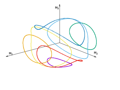
Figure 1: A few trajectories of a static Top with moments of inertia $I_{1}=1$, $I_{2}=2$, $I_{3}=3$. These trajectories were generated by a code emplying a Runge-Kutta 4th order integration scheme and step $h=0.001$. The initial data were randomly generated with the unique constraint of having all the same value of $\rho=2$. Conservation of $\rho$ and of the energy was achieved up to numerical precision.

3.2 The Throbbing Top

The mathematical description of a non-autonomous periodic Top, according to section 1, is set on the algebra

$$\mathbb{V}_{TT}\,\overset{\text{def}}{=}\,\mathcal{C}^{\infty}(\,\mathbb{T}\,\to\,\mathbb{V}_{\text{Top}}\,)\,\owns\,f=f\big{(}\overline{\boldsymbol{\mathit{M}}},t\big{)}$$ (57)

again with the bracket (52). As the time variable doesn’t enter in the bracket, $\rho$ is still a Casimir. This means that the energy, even if it is fluctuating, has to respect the bound (56). The phase space, that in the static case was the sphere $\mathbb{S}_{2}$, becomes $\mathbb{S}_{2}\times\mathbb{T}$.

We will assume that the unperturbed Hamiltonian is still given by (54). We are interested in perturbations of type

$$V=\frac{1}{2}\,\overline{\boldsymbol{\mathit{M}}}\mathsf{A}(t)\boldsymbol{\mathit{M}}$$ (58)

where $\mathsf{A}(t)$ is a $3\times 3$ diagonal matrix with time dependent coefficients. Physically, this will represent a Top for which the moments of inertia are changing in time.

The new dynamical system is

$$\dot{F}\,=\,\mathcal{H}F\,+\,\{V\}F\,,\quad\mathcal{H}\,=\,\{E\}\,+\,\partial_{t}$$ (59)

For instance, for $F=M_{i},\,i=1,2,3$ and $V$ given by (58) with

$$\mathsf{A}(t)=\begin{pmatrix}0&0&0\\ 0&\epsilon\cos(\nu t)&0\\ 0&0&0\end{pmatrix}$$ (60)

we are describing a Top with $I_{2}\,=\,I_{2}^{\emptyset}/(1+I_{2}^{\emptyset}\epsilon\cos(\nu t))$ being $I_{2}^{\emptyset}$ the static value of $I_{2}$. In figure 2 we plot some trajectories of this dynamical system. We observe the typical features of dynamical systems with cohexistence of order and chaos. The separatrices (the lines joining the hyperbolic equilibria $M_{1}=0,M_{3}=0$) disappear, and are replaced by orbits spanning a two-dimensional area. Around the elliptic equilibrium points (of coordinates respectively $M_{1}=0,M_{2}=0$ and $M_{2}=0,M_{3}=0$), some of the original trajectories are only deformed, some others are lost and replaced by a set of new equilibrium points; some of the new equilibrium points are elliptic, and new closed orbits appear around them.

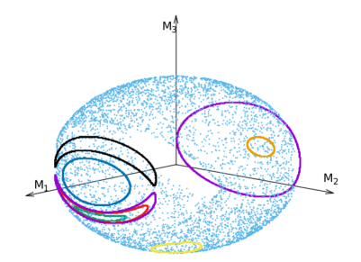
Figure 2: A few trajectories of a Throbbing Top with $I_{1}=1,\,I_{2}=2/(1+0.2\epsilon\cos(t)),\,I_{3}=3$. The initial data were generated as in 1, and the numerical method was the same as well. We checked also the conservation of $\rho$ along these trajectories.

3.3 The symmetric case

By definition a Top is symmetric if two moments of inertia are equal; here we fix $I_{1}=I_{2}\equiv I_{\perp}$. In this case the solutions of motion are uniform rotations around the third axis ($M_{3}$ is constant in time).

For a static symmetric top it is useful [10], [13] to introduce the coordinates $(\rho,X,\theta)$, $X\in(-1,1)$ and $\theta\in[0,2\pi)$, defined by

$$\{M_{1},M_{2},M_{3}\}\mapsto\{\rho,X,\theta\}\,\colon\left\{\begin{aligned} M_{1}&=\rho\sqrt{1-X^{2}}\cos(\theta)\\[3.44444pt] M_{2}&=\rho\sqrt{1-X^{2}}\sin(\theta)\\[3.44444pt] M_{3}&=\rho X\end{aligned}\right.$$ (61)

The bracket (52) restricted to $\mathbb{V}_{\text{symm}}$ becomes

$$\{F\}G=\frac{1}{\rho}\big{(}\partial_{X}\!F\,\partial_{\theta}G\,-\,\partial_{\theta}F\,\partial_{X}G\big{)}$$ (62)

The new bracket contains no derivatives in $\rho$, consistent with the definition of a Casimir. The Hamiltonian (54) becomes

$$E_{\text{symm}}\,=\,\frac{\rho^{2}}{2}\bigg{(}\frac{1-X^{2}}{I_{\perp}}+\frac{X^{2}}{I_{3}}\bigg{)}\,\equiv\,\frac{\rho^{2}}{2}\Delta\,X^{2}\,+\,\frac{\rho^{2}}{2I_{\perp}}$$ (63)

where we have set $\Delta=\frac{1}{I_{3}}-\frac{1}{I_{\perp}}$.

So we see that $X$ and $\theta$ behave like action-angle coordinates.

The coordinates $X$ and $\theta$ don’t cover the whole sphere, as the north and south poles are excluded. However, in the stationary case the poles are elliptic equilibria, so they are not very interesting for the dynamics. In the non-autonomous case the energy is still subject to the bound (56). If the bound is strengthened to strict inequalities then the dynamics will never reach the poles.

So, we restrict the algebra $\mathbb{V}_{TT}$ (defined in (57)) to the subalgebra of functions $f(X,\theta,t)$ analytic in $(X,\theta,t)$ and which respect the bounds (56) with strict inequality. The restriction to analytic functions is needed to introduce a scale of Banach norms, as will be discussed in subsection 3.4.

We start by making a further change of coordinates (sometimes called localization of $X$),

$$X\,=\,x_{0}+x\,\implies\,\partial_{X}\mapsto\partial_{x}$$ (64)

where $x_{0}\in(-1,1)$ is fixed and $x$ is sufficiently small so that $x_{0}+x\in(-1,1)$. This change of variables is simply a translation and it doesn’t affect the algebraic and metric properties that we introduced up to now. Functions in $\mathbb{V}_{\text{symm}}$ can be equivalently written as $f(x,\theta,t)$. Let us also define

$$Q\overset{\text{def}}{=}\partial^{2}_{xx}H|_{x=0}$$ (65)

so that, for instance, $\{E_{\text{symm}}\}\,=\,\rho x_{0}\Delta\partial_{\theta}+\{\tfrac{1}{2}Qx^{2}\}$

Now we will show that all the hypothesis of Lemma 1 are satisfied for the symmetric Throbbing Top, that is, by system (59) on the algebra $\mathbb{V}_{\text{symm}}$ with $E=E_{\text{symm}}$.

1. First we look for a subalgebra $\mathbb{B}$ of $\mathbb{V}_{\text{symm}}$, invariant by $\mathcal{H}$. Led again by analogy with classical mechanics, we choose

$$\mathbb{B}=\big{\{}F(\rho,x,\theta,t)\in\mathbb{V}\quad\text{s.t.}\quad F(\rho,0,\theta,t)=0,\,\partial_{x}F(\rho,0,\theta,t)=0\big{\}}$$ (66)

By definition we have $F\in\mathbb{B}\iff\mathcal{P}_{\geq 2}F_{2}=F_{2}$ (see Table 1 for the definition of $\mathcal{P}_{\geq 2}$), but neither $\{E_{\text{symm}}\}$ nor $\partial_{t}$ can decrease the degree in $x$ of a polynomial. So $\mathcal{H}\mathbb{B}\subseteq\mathbb{B}$.

$$\begin{array}[]{c}\hline\cr\hline\cr\oint\colon f(x,\theta,t)\mapsto\int_{0}^{2\pi}d\theta\int_{0}^{2\pi}dtf(x,\theta,t)\equiv f_{0,0}(x)\\[8.61108pt] \chi\overset{\text{def}}{=}1-\oint\colon f\mapsto\sum_{l,m\in\mathbb{Z}_{0}}f_{l,m}(x)e^{im\theta+ilt},\mathbb{Z}_{0}\overset{\text{def}}{=}\mathbb{Z}\backslash\{0\}\\[8.61108pt] \mathcal{P}_{k}\colon\sum_{n\geq 0}a_{n}x^{n}\mapsto a_{k}x^{k}\,\,k\in\mathbb{N},\,a_{n}\in\mathbb{R}\ \forall n\in\mathbb{N}\\[8.61108pt] \mathcal{P}_{\geq k}\colon\sum_{n\geq 0}a_{n}x^{n}\mapsto\sum_{n\geq k}a_{n}x^{n}\\[8.61108pt] \mathcal{R}_{s}\overset{\text{def}}{=}\oint\mathcal{P}_{0}+\mathcal{P}_{\geq 2}\\[8.61108pt] \mathcal{N}_{s}\overset{\text{def}}{=}\chi\mathcal{P}_{0}+\mathcal{P}_{1}\equiv 1-\mathcal{R}_{s}\\[8.61108pt] \mathcal{G}_{s}\colon f\mapsto\sum_{l,m\in\mathbb{Z}_{0}}\frac{-i\mathcal{P}_{\leq 1}f_{l,m}(x)}{\rho x_{0}\Delta m+l}e^{im\theta+ilt}\\[8.61108pt] \mathcal{A}\overset{\text{def}}{=}\Big{(}\oint Q\Big{)}^{-1}\oint\mathcal{P}_{0}(\partial_{x}-Q\partial_{\theta}\mathcal{G}_{s})\\[8.61108pt] \mathcal{K}\,\overset{\text{def}}{=}\,\rho^{2}x_{0}\Delta\mathcal{A}\,+\,\{\tfrac{1}{2}Qx^{2}\}\,x\mathcal{G}_{s}\,\big{(}\mathcal{P}_{0}\partial_{x}-\,Q\mathcal{A}-Q\partial_{\theta}\mathcal{G}_{s}\mathcal{P}_{0}\big{)}\\ \hline\cr\hline\cr\end{array}$$

Table 1: Here we group some of the operators defined on $\mathbb{V}$ and needed for the KAM algorithm. We are using the Fourier representation (76), the $1$s are to be intended as identity operators, $H$ is the Hamiltonian, and $Q$ has been defined in equation (65).

2. As a second step we build the projector $\mathcal{R}$ (and thus $\mathcal{N}=\mathbb{I}-\mathcal{R}$). We choose

$$\mathcal{R}\overset{\text{def}}{=}\mathcal{R}_{s}-\mathcal{K},\quad\mathcal{N}\overset{\text{def}}{=}\mathcal{N}_{s}+\mathcal{K}$$ (67)

where $\mathcal{R}_{s},\mathcal{N}_{s}$ and $\mathcal{K}$ are defined in table 1. It’s evident that $\mathcal{R}_{s}$ takes values in $\mathbb{B}$, and then $\mathcal{R}=\mathcal{R}_{s}-\mathcal{K}\equiv\mathcal{R}_{s}(1-\mathcal{K})$. In point (4) we show that $\mathcal{N}\mathcal{R}=0$ so we can conclude that they are both projectors.

3. The third step is to build the operator $\Gamma$. As we discussed at the beginning of section 2, it would be simpler to compute $\mathcal{G}\colon\mathbb{V}\to\mathbb{V}$ and then $\Gamma F=\{\mathcal{G}F\}$. The operator $\mathcal{G}_{s}$ from table 1 satisfies

$$\big{(}\rho x_{0}\Delta\partial_{\theta}\,+\,\partial_{t})\,\mathcal{G}_{s}F\,=\,\mathcal{N}_{s}F\,,\quad\forall F\in\mathbb{V}$$

This equation is called “homological equation” in classical mechanics. Unfortunately, the term in parenthesis above doesn’t correspond to our $\mathcal{H}$, which needs a more complicated pseudo-inverse.

4. Still making reference to table 1, consider the following operator:

$$\mathcal{G}\,=\,\mathcal{G}_{s}\,+\,\rho\,\theta\mathcal{A}\,-\,x\mathcal{G}_{s}Q(\mathcal{A}+\partial_{\theta}\mathcal{G}_{s}\mathcal{P}_{0})$$ (68)

It acts on elements of $\mathbb{V}$, but it doesn’t take values in $\mathbb{V}$, because the function $\theta$ doesn’t belong to $\mathbb{V}$. But we can formally compute

$$\Gamma f=\{\mathcal{G}f\}=\{\mathcal{G}_{s}f\}-\rho^{-1}\mathcal{A}f\partial_{x}-\{x\mathcal{G}_{s}Q(\mathcal{A}+\partial_{\theta}\mathcal{G}_{s}\mathcal{P}_{0})f\}$$ (69)

so $\Gamma$ goes from $\mathbb{V}$ to $\operatorname{der}\mathbb{V}$. So we proceed to check equation (15) that in this context reads

$$(\rho x_{0}\Delta\partial_{\theta}+\partial_{t}+\{\tfrac{1}{2}Qx^{2}\})\,(\mathcal{G}_{s}+\rho\theta\mathcal{A}-x\mathcal{G}_{s}Q(\mathcal{A}+\partial_{\theta}\mathcal{G}_{s}\mathcal{P}_{0}))f=\mathcal{N}f\\$$ (70)

We use $\{\tfrac{1}{2}Qx^{2}\}=xQ\partial_{\theta}-\tfrac{1}{2}x^{2}(\partial_{\theta}Q)\partial_{x}$ and we get

$$\chi\mathcal{P}_{\leq 1}f+\{\tfrac{1}{2}Qx^{2}\}\mathcal{G}_{s}f-x\chi\mathcal{P}_{\leq 1}Q(\mathcal{A}+\partial_{\theta}\mathcal{G}_{s}\mathcal{P}_{0})f+\underset{\bullet}{\underline{xQ\mathcal{A}f}}\\ +\underset{\sim}{\underline{\rho x_{0}\Delta\mathcal{A}f}}+\underset{\square}{\underline{\{\tfrac{1}{2}Qx^{2}\}x\mathcal{G}_{s}Q(\mathcal{A}+\partial_{\theta}\mathcal{G}_{s}\mathcal{P}_{0})f}}=(\chi\mathcal{P}_{0}+\mathcal{P}_{1})f+\underset{\sim}{\underline{\rho x_{0}\Delta\mathcal{A}f}}+\\ -\underset{\square}{\underline{\{\tfrac{1}{2}Qx^{2}\}x\mathcal{G}_{s}Q\mathcal{A}f}}+\underset{\bullet}{\underline{xQ\mathcal{A}f}}+\{\tfrac{1}{2}Qx^{2}\}x\mathcal{G}_{s}\mathcal{P}_{0}\partial_{x}f-\underset{\square}{\underline{\{\tfrac{1}{2}Qx^{2}\}x\mathcal{G}_{s}\mathcal{P}_{0}Q\partial_{\theta}\mathcal{G}_{s}f}}$$ (71)

All the terms underlined in the same way cancel among themselves, and we are left with

$$\{\tfrac{1}{2}Qx^{2}\}\mathcal{G}_{s}f+xQ\mathcal{A}f-x(\chi Q)\mathcal{A}f-x\chi Q\partial_{\theta}\mathcal{G}_{s}\mathcal{P}_{0}f\,=\,\oint\mathcal{P}_{1}f+\{\tfrac{1}{2}Qx^{2}\}x\mathcal{G}_{s}\mathcal{P}_{0}\partial_{x}f$$ (72)

Now we observe that $x\mathcal{P}_{0}\partial_{x}f=\mathcal{P}_{1}f$ so that there is a partial cancellation among the first and the latter term in the above equation, and there remains

$$\{\tfrac{1}{2}Qx^{2}\}\mathcal{G}_{s}\mathcal{P}_{0}f\,+\,x\big{(}\oint Q\big{)}\mathcal{A}f\,-\,x\chi Q\partial_{\theta}\mathcal{G}_{s}\mathcal{P}_{0}f=\,\oint\mathcal{P}_{1}f$$ (73)

Then we insert the explicit expressions of $\{\tfrac{1}{2}Qx^{2}\}$ and that of $\mathcal{A}$ as it can be found in table 1,

$$\underset{\diamond}{\underline{xQ\partial_{\theta}\mathcal{G}_{s}\mathcal{P}_{0}f}}\,+\,\underset{\triangle}{\underline{x\oint\mathcal{P}_{0}\partial_{x}f}}\,-\,\underset{\diamond}{\underline{x\oint Q\partial_{\theta}\mathcal{G}_{s}\mathcal{P}_{0}f}}\,-\,\underset{\diamond}{\underline{x\chi Q\partial_{\theta}\mathcal{G}_{s}\mathcal{P}_{0}f}}\,=\,\underset{\triangle}{\underline{\oint\mathcal{P}_{1}f}}$$ (74)

Again we underlined in the same way all the terms that cancels out. We conclude that equation (15) is satisfied.

5. Here we show that $\mathcal{G}\mathcal{R}=0$, so that $\mathcal{H}\mathcal{G}\mathcal{R}=\mathcal{NR}=0$. We start by writing explicitly

$$\mathcal{G}\mathcal{R}=\Big{(}\mathcal{G}_{s}+\theta\mathcal{A}-x\mathcal{G}_{s}Q(\mathcal{A}+\partial_{\theta}\mathcal{G}_{s}\mathcal{P}_{0})\Big{)}\Big{(}\mathcal{R}_{s}-\rho\Delta x_{0}\mathcal{A}-\{\tfrac{1}{2}Qx^{2}\}x\mathcal{G}_{s}(\mathcal{P}_{0}\partial_{x}-Q\mathcal{A}-Q\partial_{\theta}\mathcal{G}_{s}\mathcal{P}_{0})\Big{)}$$

Next we observe that, by applying the following equalities

$$\mathcal{G}_{s}\mathcal{R}_{s}\propto\chi\mathcal{P}_{\leq 1}(\oint\mathcal{P}_{0}+\mathcal{P}_{\geq 2}))=0$$

$$\mathcal{AR}_{s}f=\Big{(}\oint Q\Big{)}^{-1}\Big{(}\oint\mathcal{P}_{0}\partial_{x}\mathcal{P}_{\geq 2}-\oint Q\partial_{\theta}\mathcal{G}_{s}\mathcal{R}_{s}\Big{)}=0$$

$$\mathcal{AA}\propto\mathcal{A}\oint\mathcal{P}_{0}=0$$

$$\mathcal{G}_{s}\mathcal{A}\propto\mathcal{G}_{s}\oint\mathcal{P}_{0}=0$$

many terms cancel, and we are left with

$$\mathcal{G}\mathcal{R}=\Big{[}-\mathcal{G}_{s}-\theta\mathcal{A}+x\mathcal{G}_{s}Q(\mathcal{A}+\partial_{\theta}\mathcal{G}_{s}\mathcal{P}_{0})\Big{]}\,\underbrace{\{\tfrac{1}{2}Qx^{2}\}x\mathcal{G}_{s}(\mathcal{P_{0}}\partial_{x}-Q\mathcal{A}-Q\partial_{\theta}\mathcal{G}_{s}\mathcal{P}_{0})}_{\in\operatorname{ran}(\mathcal{R}_{s})}=0$$ (75)

We can conclude that Proposition 1 can be applied to the symmetric periodic Throbbing Top.

3.4 A scale of Banach norms for $\mathbb{V}_{\text{symm}}$

Functions in $\mathbb{V}_{\text{symm}}$ are analytic and thus admit the Fourier representation

$$F(x,\theta,t)\,=\,\sum_{l,m\in\mathbb{Z}}F_{l,m}(x)\,e^{ilt+im\theta}$$ (76)

Analyticity allows to build a complex extension $(-1,1)$, the domain of $X$ (and of $x$). Let $\mathbb{B}_{r}(X)\subseteq\mathbb{C}$ be a ball in the complex plane, of radius $r\in\mathbb{R}_{+}$ centered at $X$. The radius $r$ has to be sufficiently small so that $|X\pm r|<1$. Then we define the set

$$\mathbb{A}_{r}\overset{\text{def}}{=}\bigcup_{X\in(-1,1)}\mathbb{B}_{r}(X)$$ (77)

The algebra $\mathbb{V}_{\text{symm}}$ is a subalgebra of

$$\mathbb{V}_{r}\,\overset{\text{def}}{=}\,\mathcal{C}^{\infty}(\mathbb{A}_{r}\otimes\mathbb{T}^{2})$$ (78)

for any $r$. Moreover, we restrict to the subset of analytic functions, so that each space $\mathbb{V}_{r}$ is endowed with the Banach norm

$$\big{\|}f\big{\|}_{r}\overset{\text{def}}{=}\sum_{l,m\in\mathbb{Z}}\big{|}f_{l,m}\big{|}_{r}\,e^{r(|l|+|m|)}\,,\quad\big{|}f_{l,m}\big{|}_{r}\overset{\text{def}}{=}\sup_{X\in\mathbb{A}_{r}}|f(X)|$$ (79)

So we have a scale of Banach norms $\{\big{\|}\quad\big{\|}_{r}\}_{r\in\mathbb{R}_{+}}$ and a scale of Banach spaces $\{\mathbb{V}_{r}\}_{r\in\mathbb{R}_{+}}$. Some properties of these norms are collected in the following Proposition (the proof can be easily reconstructed by adapting the proof of Lemma 1 of [12]).

Proposition 3.

Consider the Lie algebra $\mathbb{V}_{\text{symm}}$ with the scale of Banach norms (79). Let $r,\delta,d\in\mathbb{R}_{+}$ with $d+\delta<r$. Let also $W\in\mathbb{V}_{r},\,Z\in\mathbb{V}_{r-\delta}$ . Then

$$\|\partial_{X}W\|_{r-d}\,\leq\,\frac{1}{d}\|W\|_{r}$$ (80)

$$\|\partial_{\theta}W\|_{r-d}\,\leq\,\frac{1}{ed}\|W\|_{r}$$ (81)

$$\|\{W\}Z\|_{r-d-\delta}\,\leq\,\frac{2}{\rho ed(d+\delta)}\|W\|_{r}\|Z\|_{r-\delta}$$ (82)

Instead in the appendix A we prove the following

Proposition 4.

Consider the Lie algebra $\mathbb{V}_{\text{symm}}$ with the scale of Banach norms (79). Let $V,Q\in\mathbb{V}_{r}$ for some $r\in\mathbb{R}_{+}$. Define two operators $\mathcal{R},\mathcal{N}$ by (67) and an operator $\Gamma$ by (69). Assume there exist real numbers $\gamma,\rho,\Delta>0$, $\tau>1$, $0<q<1$ and $-1<x_{0}<1$ such that:

1. $x_{0},\rho,\Delta,\gamma$ and $\tau$ satisfy $\,\big{|}\,\rho\Delta x_{0}m\,+\,l\,\big{|}\,\geq\,\gamma\,\big{(}|l|+|m|\big{)}^{-\tau},\quad\forall l,m\in\mathbb{Z}_{0}$;

2. $|Q_{00}|\,\geq\,q$;

3. $\|Q\|_{r}\,\leq\,q^{-1}$;

Then $\forall d,\delta\in\mathbb{R}_{+},d+\delta<r$ and $\,\forall W\in\mathbb{V}_{r}\,,\,\forall Z\in\mathbb{V}_{r-\delta}$, the following inequalities hold

$$\|(\Gamma W)Z\|_{r-\delta-d}\,\leq\,\frac{C\,\|W\|_{r}\,\|Z\|_{r-\delta}}{q^{3}d(d+\delta)^{2\tau+2}}$$ (83)

$$\|\mathcal{N}W\|_{r-\delta}\leq\frac{\tilde{C}\,\|W\|_{r}}{q^{3}\,\delta^{2\tau+3}}$$ (84)

$$\|\mathcal{R}W\|_{r-\delta}\leq\frac{\tilde{C}\,\|W\|_{r}}{q^{3}\,\delta^{2\tau+3}}$$ (85)

where $C$ and $\tilde{C}$ are constants depending on $\tau,\gamma,e,q,\rho,\delta,d$.

The inequalities (83) and (84), are respectively of type (i) and (ii) of Proposition 2, with

$$\Lambda(d,\delta)\,=\,\frac{C}{q^{3}\,d\,(d+\delta)^{2\tau+2}}\,,\qquad\Xi(\delta)\,=\,\frac{\tilde{C}}{q^{3}\,\delta^{2\tau+3}}$$ (86)

We see that some extra hypothesis on $Q$ and on the product $\rho\Delta x_{0}$ are required. In particular condition (1) of Proposition 4 is usually called the “Diophantine condition”. Instead hypothesis (2) goes generally under the name of “non-degeneracy condition”. Finally, condition (iii) of Proposition 2 defines the parameter $\epsilon$, that in this case equals

$$\epsilon_{\mu} =\,\frac{1}{2}\sup_{n\in\mathbb{N}}\bigg{(}\frac{1}{n!}\,\prod_{j=1}^{n}\Lambda\Big{(}\tfrac{\mu}{n},\tfrac{(j-1)\mu}{n}\Big{)}\bigg{)}^{-1/n}\,=\,\frac{1}{2}\sup_{n\in\mathbb{N}}\bigg{(}\frac{1}{n!}\,\prod_{j=1}^{n}\frac{C}{q^{3}\,\tfrac{\mu}{n}\,\big{(}\tfrac{j\mu}{n}\big{)}^{2\tau+2}}\bigg{)}^{-1/n}\,=$$

$$=\,\frac{q^{3}\mu^{2\tau+3}}{2\,C}\,\sup_{n\in\mathbb{N}}\Big{(}\frac{n^{n}}{n!}\Big{)}^{2\tau+3}\,=\,\frac{q^{3}\mu^{2\tau+3}}{2\,C}\,\sup_{n\in\mathbb{N}}\Big{(}e^{1-1/n}\Big{)}^{2\tau+3}=\,\frac{q^{3}\mu^{2\tau+3}}{2\,C}$$

So, if $q,\mu,\tau$ and $C$ are chosen so that $0<\epsilon_{\mu}<\infty$, we can conclude that also Proposition 2 applies to the symmetric and periodic Throbbing Top.

3.5 A KAM theorem for the Symmetric Throbbing Top

Now we prove a KAM theorem for the symmetric Throbbing Top by iteratively applying Proposition 1.

Theorem 1.

Consider the dynamical system (59) on the algebra $\mathbb{V}_{\text{symm}}$ and with $E=E_{\text{symm}}$ (Throbbing Top). Define $Q$ as in equation (65) and $\rho,\Delta,\gamma,\tau,q\in\mathbb{R}_{+}$ as in Proposition 4. Then there exist $\epsilon_{0},r\in\mathbb{R}_{+}$ such that if $\|V\|_{r}\leq\epsilon$, the for a large class of initial data, the trajectories of the Throbbing Top can be mapped to trajectories of a static Top $\mathcal{H}_{\infty}$.

Proof.

We have shown in the previous section that Proposition 1 can be applied to the symmetric and periodic Throbbing Top, by choosing $\mathbb{B}$ as in (66), $\mathcal{R}$ as in (67) and $\Gamma$ as in (69). Thus by formula (20) we can map $\mathcal{H}+\{V\}$ into $\mathcal{H}_{*}+\{V_{*}\}$. This is possible, in particular, if $X(t=0)=x_{0}$ satisfy the Diophantine condition (1) of Proposition 4.. We have to choose a loss $\mu_{0}\in\mathbb{R}_{+}$ such that $\mu_{0}<r/3$, so that $\|V_{*}\|_{r-3\mu}<\kappa\,\epsilon_{0}^{2}$.

Now we want to show that Proposition 1 can be applied to $\mathcal{H}_{*}+\{V_{*}\}\equiv\,\mathcal{H}+\{RV\}+\{V_{*}\}$, so with the same values of $\rho,\Delta$ and $x_{0}$ but with the replacements

$$Q\,\to\,Q^{*}\overset{\text{def}}{=}Q+\partial^{2}_{xx}(\mathcal{R}V)\,,\quad\quad r\to r_{*}\equiv r-\mu\,,\quad\quad V\to V_{*}$$ (87)

We need to verify that there exist a new constant $q_{*}$ for which hypothesis (2) and (3) of Proposition 4 are again satisfied. By using inequality (85) of Proposition 4,

$$\|Q^{*}-Q\|_{r-\mu}\,=\,\|\partial^{2}_{xx}\mathcal{R}V\|_{r-\mu}\,\leq\,\frac{2}{r^{2}}\|\mathcal{R}V\|_{r}\,\leq\,\frac{2\,\epsilon\,\tilde{C}}{r^{2}q^{3}\mu^{2\tau+3}}$$ (88)

where we used equations (80), (85), and the Cauchy inequality (38). In the same way

$$|Q^{*}_{0,0}-Q_{0,0}|\,=\,\Big{|}\oint\partial^{2}_{xx}\mathcal{R}V\Big{|}\,\leq\,\frac{2}{r^{2}}\Big{|}\oint\mathcal{R}V\Big{|}_{r}\,\leq\,\frac{2\,\epsilon\,\tilde{C}}{r^{2}q^{3}\mu^{2\tau+3}}$$ (89)

So we have

$$\|Q^{*}\|_{r-\mu}\,\leq\,\|Q\|_{r_{0}-\mu}\,+\,\|Q^{*}-Q\|_{r_{0}-\mu}\,\leq\,\frac{1}{q}\,+\,\frac{\epsilon\tilde{C}}{r^{2}q^{3}\mu^{2\tau+3}}\,\leq\,\frac{1}{q-\frac{\epsilon\tilde{C}}{r^{2}q^{3}\mu^{2\tau+3}}}\,\equiv\,\frac{1}{q_{*}}$$ (90)

where the last inequality holds as long as

$$0\leq\frac{\epsilon\tilde{C}}{r^{2}q^{3}\mu^{2\tau+}}\leq q\leq 1$$ (91)

This condition is to be confronted with formula (3.4); they are compatible if

$$q\,\,\geq\,\tilde{C}/(C\,r^{2})$$ (92)

At the same time, $|Q_{0,0}|\,\leq\,|Q_{0,0}-Q^{*}_{0,0}|\,+\,|Q^{*}_{0,0}|$ so

$$|Q^{*}_{0,0}|\,\geq\,|Q_{0,0}|-|Q^{*}_{0,0}-Q_{0,0}|\,\geq\,q\,-\,\frac{\epsilon\tilde{C}}{q^{3}\mu^{2\tau+5}}\,\equiv\,q_{*}$$ (93)

So Proposition 1 can be applied to $\mathcal{H}_{*}+\{V_{*}\}$. We may build a sequence of dynamical systems by

$$e^{[\Gamma_{i}V_{i}]}(\mathcal{H}_{i}+\{V_{i}\})=\mathcal{H}_{i+1}+\{V_{i+1}\}$$ (94)

$$V_{0}\equiv V\,,\quad Q^{0}\equiv Q\,,\quad\mathcal{H}_{i}=x_{0}\rho\Delta\partial_{\theta}+\partial_{t}+\{\tfrac{1}{2}Q^{i}x^{2}\}$$ (95)

$$\Gamma_{i}f=\{\mathcal{G}f\}=\{\mathcal{G}_{s}f\}-\rho^{-1}\mathcal{A}_{i}f\partial_{x}-\{x\mathcal{G}_{s}Q^{i}(\mathcal{A}_{i}+\partial_{\theta}\mathcal{G}_{s}\mathcal{P}_{0})f\}$$ (96)

$$\mathcal{A}_{i}=\Big{(}\oint Q^{i}\Big{)}^{-1}\oint\mathcal{P}_{0}(\partial_{x}-Q^{i}\partial_{\theta}\mathcal{G}_{s}\mathcal{P}_{0}).$$ (97)

The sequence converges to the static Top

$$\mathcal{H}_{\infty}\,=\,\mathcal{H}\,+\,\sum_{i=0}^{\infty}\mathcal{R}_{i}V_{i}$$ (98)

To show that the sequence exists, we need three sequences $\{\epsilon_{i},\mu_{i},q_{i}\}_{i\in\mathbb{N}}$ such that

$$\Gamma_{i}V_{i}\colon\mathbb{V}_{r_{i}}\to\mathbb{V}_{r_{i+1}}\,,\quad\|Q^{i}\|_{r_{i}}<(q_{i})^{-1}\,,\quad|{Q^{i}}_{0,0}|>q_{i}\,,\quad\|V_{i}\|_{r_{i}}<\epsilon_{\mu_{i}}^{2}$$ (99)

where $r_{i}\equiv r-\sum_{j=1}^{i-1}\mu_{j}$. Moreover they must satisfy:

1. $\epsilon_{i}\,=\,q^{3}_{i}{\mu_{i}}^{2\tau+3}/(2\,C)$ as we computed in section 3.4;

2. $q_{i}\,\geq\tilde{C}/(Cr_{i}^{2})$, coherently with equation (92);

3. $0<\mu_{i}<\tfrac{r_{i}}{3}$, as required by Proposition 1;

4. $\sum_{i=1}^{\infty}\mu_{i}<r$, to ensure that

   $$r_{\infty}=r-\sum_{j=1}^{\infty}\mu_{j}>0$$

   and so that the operator $\mathcal{H}_{\infty}$ is well defined on $\mathbb{V}_{r_{\infty}}$;

5. $\lim_{i\to\infty}\epsilon_{i}=0$, so we can conclude that $V_{\infty}\overset{\text{def}}{=}\lim_{i\to\infty}V_{i}=0$;

6. $0<q_{\infty}<q_{i}<1,\quad\forall i\in\mathbb{N}$ as required by Proposition 4;

We choose

$$\epsilon_{i}\,=\,\frac{\epsilon_{0}}{(i+1)^{2(2\tau+3)}},\qquad\mu_{i}\,=\,\frac{1}{(1+i)^{2}}\bigg{(}\frac{2\,C\,\epsilon_{0}}{q_{i}^{3}}\bigg{)}^{\tfrac{1}{2\tau+3}}$$ (100)

so that condition (a) is satisfied. Also condition (e) is evidently satisfied. Now we compute

$$\sum_{i=0}^{\infty}\mu_{i}\,=\,\sum_{i=0}^{\infty}\frac{1}{(1+i)^{2}}\bigg{(}\frac{2\,C\,\epsilon_{0}}{q_{i}^{3}}\bigg{)}^{\tfrac{1}{2\tau+3}}\,\leq\,\bigg{(}\frac{2\,C\,\epsilon_{0}}{q_{\infty}^{3}}\bigg{)}^{\tfrac{1}{2\tau+3}}\,\sum_{i=1}^{\infty}\frac{1}{i^{2}}\,\leq\,\frac{\pi^{2}}{6}\bigg{(}\frac{2\,C\,\epsilon_{0}}{q_{\infty}^{3}}\bigg{)}^{\tfrac{1}{2\tau+3}}$$ (101)

Both conditions (c) and (d) are satisfied by imposing $\sum_{i=0}^{\infty}\mu_{i}<r/3$ and, by the result above, we get

$$\bigg{(}\frac{2\,C\,\epsilon_{0}}{q_{\infty}^{3}}\bigg{)}^{\frac{1}{2\tau+3}}\leq\,\frac{2\,r}{\pi^{2}}$$ (102)

Then for the sequence $\{q_{i}\}_{i\in\mathbb{N}}$ we make the ansatz

$$q_{i}=q_{i-1}\Big{(}1-\frac{1}{(i+1)^{2}}\Big{)}=q_{0}\prod_{j=2}^{i+1}\Big{(}1-\frac{1}{j^{2}}\Big{)}$$ (103)

By taking the logarithm of both sides, and using that $\log(1-x)\geq-\log(4)x$ for $x\in[\tfrac{1}{2},1]$, we get

$$\log(q_{i})=\log(q_{0})+\sum_{j=2}^{i+1}\log\Big{(}1-\frac{1}{j^{2}}\Big{)}\geq\\ \geq\log(q_{0})-\sum_{j=2}^{i+1}\frac{\log(4)}{j^{2}}\geq\log(q_{0})-\sum_{j=1}^{\infty}\frac{\log(4)}{j^{2}}=\log(q_{0}\,2^{-\pi^{2}/3})$$ (104)

We set $q_{\infty}=q_{0}\,2^{-\pi^{2}/3}$ and $q_{0}<1$ so condition (f) is satisfied. If we plug this value for $q_{\infty}$ into equation (102) we get

$$\epsilon_{0}\,\leq\,\frac{q_{0}^{3}}{C}\,\bigg{(}\frac{r}{\pi^{2}}\bigg{)}^{2\tau+3}2^{(4+2\tau-\pi^{2})(2\tau+3)/(1-\pi^{2})}$$ (105)

Finally, we rewrite condition (b) as $r^{2}\geq\tilde{C}/(qC)$ and, being $1/q\geq 1$, we get a lower bound on $r$,

$$r\geq\sqrt{\tilde{C}/C}$$ (106)

∎

4 Conclusions

So, in this paper we have provided an algorithm to perform perturbation theory for a Hamiltonian system on a Lie algebra. We assume to have a flow (unperturbed) that preserves some Lie subalgebra of the Lie algebra. When a perturbation is added to the given flow, the subalgebra is not preserved anymore. However, it is possible to conjugate the perturbed flow to a new one, that preserves the same subalgebra of the unperturbed system, up to terms quadratic in the perturbation.

while extending its scope beyond the original one. Variants of the original theorem of Kolmogorov [14] have already been proposed: for classical systems without action-angle coordinates [9], for classical system with degeneracy in the Hamiltonian [3], [22], or in theorin the volume preserving maps and flows [15]; all of these cases are encompassed in our formula. Nevertheless we can do more, and apply our method to non-canonical Poisson systems, which are gaining increasing importance in physics, since some pioneering works in the 1980ies [20], [16].

We have applied our theorem to the simple example of a non-autonomous symmetric Top. The Top is a non-canonical Hamiltonian system with a degenerate bracket (52), which is not written in canonical coordinates. However, with a change of variables we can reduce it to a canonical form. When the moments of inertia have a prescribed time-dependence, the system becomes non-autonomous and is described by another angle variable (if it is periodically time-dependent). One novelty with respect to classical mechanics is that the phase space has not the structure of a cotangent bundle. We have shown that our formula can be iteratively applied, to prove a KAM theorem for this dynamical system.

While on the one side we have shown that our method fits in a typical KAM scheme, even if the system under consideration fails the hypothesis of non-degeneracy, we have not used many potentialities of our method. For instance, we have introduced a set of canonical coordinates: it would be interesting to reconsider the problem in the coordinates $(\overline{\boldsymbol{\mathit{M}}},t)$: this can be done with our method, after a proper choice of the subalgebra $\mathbb{B}$ and of the operators $\mathcal{R}$ and $\Gamma$. However, we think that the most interesting development would be to write an iteration mechanism that works on any Lie algebra to provide an algebraic KAM theorem.

Appendix A Proof of Proposition 4

By definition,

$$(\Gamma W)Z\,=\,\{\mathcal{G}_{s}W\}Z-(\mathcal{A}W)\,\partial_{x}Z-\{x\mathcal{G}_{s}Q\mathcal{A}W\}Z-\{x\mathcal{G}_{s}Q\partial_{\theta}\mathcal{G}_{s}\mathcal{P}_{0}W\}Z$$ (107)

We will study each of the four terms on the r.h.s. separately. About the first one,

$$\|\{\mathcal{G}_{s}W\}Z\|_{r-\delta-d}\,=$$

$$=\,\sum_{L,M\in\mathbb{Z}} \frac{e^{(r-\delta-d)(|L|+|M|)}}{\rho}\bigg{|}\sum_{l,m\in\mathbb{Z}_{0}}\frac{W_{l,m,1}\,(M-m)\,Z_{L-l,M-m}\,-\,m\,(\mathcal{P}_{\leq 1}W_{l,m})\,\partial_{x}Z_{L-l,M-m}}{x_{0}\Delta\rho m+l}\bigg{|}_{r-d}\leq$$

$$\leq \,\sum_{L,M\in\mathbb{Z};l,m\in\mathbb{Z}_{0}}\,e^{(r-\delta-d)(|L-l|+|M-m|)}\,e^{(r-\delta-d)(|l|+|m|)}\frac{(|m|+|l|)^{\tau}}{\gamma\rho}\,\times$$

$$\,\times\bigg{(}|W_{l,m,1}|_{r-\delta-d}\,|M-m|\,|Z_{L-l,M-m}|_{r-\delta-d}\,-\,|m|\,\big{|}\mathcal{P}_{\leq 1}W_{l,m})\big{|}_{r-\delta-d}\,\big{|}\partial_{x}Z_{L-l,M-m}\big{|}\bigg{)}\bigg{|}_{r-\delta-d}\leq$$

$$\leq \,\frac{1}{\rho\gamma}\sum_{L,M,l,m\in\mathbb{Z}}e^{r(|l|+|m|)}\,\bigg{(}\frac{1}{ed}\,\Big{(}\frac{\tau}{e(d+\delta)}\Big{)}^{\tau}e^{(r-\delta)(|L-l|+|M-m|)}\,\frac{|W_{l,m}|_{r}}{d+\delta}\,|Z_{L-l,M-m}|_{r-\delta-d}\,+$$

$$+\ \Big{(}\frac{\tau+1}{e(d+\delta)}\Big{)}^{\tau+1}\,e^{(r-\delta-d)(|L-l|+|M-m|)}\,|W_{l,m}|_{r-\delta-d}\,\frac{|Z_{L-l,M-m}|_{r-\delta}}{d}\bigg{)}\leq$$

In going from the 4th to the 5th line we used the condition (1). Now

$$\|\{\mathcal{G}_{s}W\}Z\|_{r-\delta-d}\,\leq\,\frac{\tau^{\tau}+(\tau+1)^{(\tau+1)}}{\gamma\rho e^{\tau+1}(d+\delta)^{\tau+1}d}\,\|W\|_{r}\,\|Z\|_{r-\delta}\equiv\frac{C_{1}}{(d+\delta)^{\tau+1}d}\,\|W\|_{r}\,\|Z\|_{r-\delta}$$ (108)

and in the last passage we introduced a constant $C_{1}$ for conciseness. Next we consider

$$\mathcal{A}W =\,\frac{1}{Q_{0,0}}\bigg{(}\,\mathcal{P}_{0}\,\sum_{n\geq 0}\,(n+1)\,W_{0,0,n+1}\,x^{n}-\,\oint\sum_{L,M\in\mathbb{Z};l,m\in\mathbb{Z}_{0}}\,\frac{me^{iLt+iM\theta}}{x_{0}\rho\Delta m+l}\,Q_{L-l,M-m}\,W_{l,m,0}\bigg{)}\,=$$

$$=\,\frac{W_{0,0,1}}{Q_{0,0}}\,-\,\frac{1}{Q_{0,0}}\sum_{l,m\in\mathbb{Z}_{0}}\frac{m}{x_{0}\rho\Delta m+l}\,Q_{-l,-m}\,W_{l,m,0}$$

So that

$$|\mathcal{A}W| \leq\ \Big{|}\frac{W_{0,0,1}}{Q_{0,0}}\Big{|}+\sum_{l,m\in\mathbb{Z}_{0}}\Big{|}\frac{mQ_{-l,-m}W_{l,m,0}}{Q_{0,0}(x_{0}\rho\Delta m+l)}\Big{|}\leq$$

$$\leq\ \frac{1}{q}\,\|\partial_{x}W_{0,0}\|_{r-\delta-d}\,+\,\frac{1}{q\gamma}\,\sum_{l,m\in\mathbb{Z}_{0}}\,(|m|+|l|)^{(\tau+1)}\,\|\mathcal{P}_{0}W\|_{r}\,e^{-r(|m|+|l|)}\,|Q_{-l,-m}|$$

where we used $|\mathcal{P}_{0}W_{l,m}|_{r}\leq\|\mathcal{P}_{0}W\|_{r}e^{-r(|l|+|m|)}$; also, in passing from the first to the second line we employed hypothesis (2). Continuing:

$$|\mathcal{A}W| \leq\ \frac{\|W\|_{r}}{q(d+\delta)}+\,\frac{(\tau+1)^{\tau+1}}{q\gamma(er)^{\tau+1}}\|W\|_{r}\sum_{l,m\in\mathbb{Z}_{0}}|Q_{l,m}|\leq$$

$$\leq\ \frac{\|W\|_{r}}{q(d+\delta)}\,+\,\frac{(\tau+1)^{\tau+1}}{q^{2}\gamma(er)^{\tau+1}}\|W\|_{r}\leq\ \frac{C_{2}\|W\|_{r}}{q^{2}(d+\delta)^{\tau+1}}$$

where in the last passage we used $\delta+d\leq r$ so that $r^{-1}\leq(d+\delta)^{-1}$, and $C_{2}$ is a constant. Then for the second term of equation (107) we have

$$\|(\mathcal{A}W)\partial_{x}Z\|_{r-\delta-d}\,\leq\,\sum_{l,m\in\mathbb{Z}}e^{r(|l|+|m|)}\,|aW|\,\frac{1}{d}\,|Z_{l,m}|_{r-\delta}\,\leq\,\frac{C_{2}\|W\|_{r}\|Z\|_{r-\delta}}{q^{2}\,d\,(d+\delta)^{\tau+1}}$$ (109)

The third term of equation (107) reads

$$\{x\mathcal{G}_{s}Q\mathcal{A}W\}Z\,=\,\frac{1}{\rho}\sum_{L,M\in\mathbb{Z}}\,e^{iLt+iM\theta}(\mathcal{A}W)\,\sum_{l,m\in\mathbb{Z}_{0}}\Big{(}\footnotesize{\frac{Q_{l,m}\,(M-m)\,Z_{L-l,M-m}\,-\,x\,m\,Q_{l,m}\,\partial_{x}Z_{L-l,M-m}}{x_{0}\rho\Delta m+l}}\Big{)}$$

so that

$$\big{\|}\{x\mathcal{G}_{s}Q \mathcal{A}W\}Z\big{\|}_{r-\delta-d}\,\leq$$

$$\leq \,\frac{|\mathcal{A}W|}{\rho}\,\sum_{L,M\in\mathbb{Z}}\,e^{(r-\delta-d)(|L|+|M|)}\,\bigg{|}\sum_{l,m\in\mathbb{Z}_{0}}\frac{Q_{l,m}\,(M-m)\,Z_{L-l,M-m}\,-\,x\,m\,Q_{l,m}\,\partial_{x}Z_{L-l,M-m}}{x_{0}\rho\Delta m+l}\bigg{|}_{r-\delta-d}\,\leq$$

$$\leq \,\frac{|\mathcal{A}W|}{\rho\gamma}\,\sum_{L,M,l,m\in\mathbb{Z}}\,e^{(r-\delta-d)(|L-l|+|M-m|)}\,\,e^{(r-\delta-d)(|l|+|m|)}|Q_{l,m}|\times$$

$$\,\times\bigg{(}|M-m|\,\frac{(|m|+|l|)^{\tau}}{\gamma}\,|Z_{L-l,M-m}|_{r-\delta-d}\,+\,|x|_{r-\delta-d}\,\,\big{|}\partial_{x}Z_{L-l,M-m}\big{|}_{r-\delta-d}\,\frac{(|m|+|l|)^{\tau+1}}{\gamma}\,\bigg{)}\leq$$

$$\leq \frac{|\mathcal{A}W|}{\rho\gamma}\,\bigg{(}\frac{1}{ed}\,\|Z\|_{r-\delta}\,\Big{(}\frac{\tau}{e(d+\delta)}\Big{)}^{\tau}\|Q\|_{r}\,+\,\frac{|r|}{d}\,\Big{(}\frac{\tau+1}{e(d+\delta)}\Big{)}^{\tau+1}\|Z\|_{r-\delta}\|Q\|_{r}\bigg{)}\,\leq\,\,\frac{C_{3}\|W\|_{r}\|Z\|_{r-\delta}}{q^{3}\,d\,(d+\delta)^{2\tau+2}}$$

where $C_{3}$ is another constant.

Finally, the fourth term of equation (107) is

$$\{x \mathcal{G}_{s}Q\partial_{\theta}\mathcal{G}_{s}\mathcal{P}_{0}W\}Z\,=\,\bigg{\{}x\mathcal{G}_{s}\sum_{L,M,l,m\in\mathbb{Z}_{0}}\,e^{iLt+iM\theta}\frac{mW_{l,m,0}Q_{L-l,M-m}}{x_{0}\rho\Delta m+l}\,\sum_{l_{1},m_{1}\in\mathbb{Z}}Z_{l_{1},m_{1}}e^{il_{1}t+im_{1}\theta}\bigg{\}}\,=$$

$$= \,\sum_{L_{1},M_{1}\in\mathbb{Z};L,M,l,m\in\mathbb{Z}_{0}}\,e^{iL_{1}t+iM_{1}\theta}\frac{m\,W_{l,m}\,Q_{L-l,M-m}\,(M_{1}-M)\,Z_{L_{1}-L,M_{1}-M}\,-\,x\,M\,m\,W_{l,m}\,Q_{L-l,M-m}\,\partial_{x}Z_{L_{1}-L,M_{1}-M}}{\rho(x_{0}\rho\Delta M+L)(x_{0}\rho\Delta m+l)}$$

and so

$$\|\{x\mathcal{G}_{s}Q\partial_{\theta}\mathcal{G}_{s}\mathcal{P}_{0}W\}Z\|_{r-\delta-d}\leq\\ \leq\sum_{L_{1},M_{1},L,M,l,m\in\mathbb{Z}}\bigg{(}e^{(r-\delta-d)(|L_{1}-L|+|M_{1}-M|)}\,e^{(r-\delta-d)(|L|+|M|)}\,|W_{l,m,0}|\,|Q_{L-l,M-m}|\,\frac{(|m|+|l|)^{\tau+1}}{\rho\gamma^{2}}\times\\[4.30554pt] \times\Big{(}|M_{1}-M|\,|Z_{L_{1}-L,M_{1}-M}|\,(|M|+|L|)^{\tau}\,+\,|x|(|M|+|L|)^{\tau+1}|\partial_{x}Z_{L_{1}-L,M_{1}-M}|_{r-\delta-d}\bigg{)}\,\leq\\[4.30554pt] \leq\frac{\|Z\|_{r-\delta}}{q\rho\gamma^{2}de^{\tau+1}}\,\|W\|_{r}\bigg{(}\bigg{(}\frac{2\tau}{d+\delta}\bigg{)}^{\tau}\bigg{(}\frac{2(\tau+1)}{e(d+\delta)}\bigg{)}^{\tau+1}+|r|\bigg{(}\frac{2(\tau+1)}{d+\delta}\bigg{)}^{\tau+1}\bigg{(}\frac{2(\tau+1)}{e(d+\delta)}\bigg{)}^{\tau+1}\bigg{)}\equiv\\[4.30554pt] \,\equiv\,\frac{C_{4}\|W\|_{r}\|Z\|_{r-\delta}}{q\,d\,(d+\delta)^{2\tau+1}}$$ (110)

with a fourth constant $C_{4}$. By defining

$$C\,=\,(C_{1}\,q^{3}+C_{2}\,q)(d+\delta)^{\tau+1}+C_{3}+(d+\delta)q^{2}C_{4}$$ (111)

we end up with the thesis.

To prove the second and third inequalities, we start by observing that

$$\|\mathcal{N}_{s}V\|_{r-\mu}=\|\chi\mathcal{P}_{0}V+\mathcal{P}_{1}V\|_{r-\mu}\leq\|V\|_{r-\mu}$$ (112)

$$\|\mathcal{R}_{s}V\|_{r-\mu}=\|\oint\mathcal{P}_{0}V+\mathcal{P}_{2}V\|_{r-\mu}\leq\|V\|_{r-\mu}$$ (113)

Then we consider

$$\|\mathcal{K}V\|_{r-\mu}\,\leq\,|x_{0}\Delta\rho\mathcal{A}V|\,+\,\big{\|}\{\tfrac{1}{2}Qx^{2}\}x\mathcal{G}_{s}(\mathcal{P}_{0}\partial_{x}-Q\mathcal{A}-Q\partial_{\theta}\mathcal{G}_{s}\mathcal{P}_{0})V\big{\|}_{r-\mu}$$ (114)

By (109),

$$|x_{0}\Delta\rho\mathcal{A}V|\,\leq\,|x_{0}|\,\rho\Delta\,\big{|}\mathcal{A}V\big{|}\,\leq\,\rho\Delta\,\frac{C_{2}}{q^{2}\,\mu^{\tau+1}}\,\|V\|_{r}$$ (115)

To the next term we apply equation (82) of Proposition 3 with $\delta=d=\mu/2$,

$$\big{\|}\{\tfrac{1}{2}Qx^{2}\}x\mathcal{G}_{s}(\mathcal{P}_{0}\partial_{x}-Q\mathcal{A}-Q\partial_{\theta}\mathcal{G}_{s}\mathcal{P}_{0})V\big{\|}_{r-\mu}\leq\\ \leq\frac{4}{\rho e\mu^{2}}\big{\|}\tfrac{1}{2}Qx^{2}\big{\|}_{r}\,\big{\|}x\mathcal{G}_{s}(\mathcal{P}_{0}\partial_{x}-Q\mathcal{A}-Q\partial_{\theta}\mathcal{G}_{s}\mathcal{P}_{0})V\big{\|}_{r-\mu/2}$$ (116)

We have

$$\big{\|}\tfrac{1}{2}Qx^{2}\big{\|}_{r}\,\leq\,\tfrac{1}{2}\|Q\|_{r}|x^{2}|_{r}\leq(2q)^{-1}$$ (117)

and

$$\big{\|}x\mathcal{G}_{s} \mathcal{P}_{0}\partial_{x}V\big{\|}_{r-\mu/2}\,=\sum_{l,m\in\mathbb{Z}_{0}}\Big{|}\frac{V_{lm1}x}{x_{0}\rho\Delta m+l}\Big{|}_{r-\tfrac{\mu}{2}}\,e^{(r-\mu/2)(|l|+|m|)}\leq$$

$$\leq\,\sum_{l,m\in\mathbb{Z}_{0}}|V_{lm1}x|_{r-\mu/2}\,\big{(}|m|+|l|\big{)}^{\tau}\gamma^{-1}\,e^{(r-\mu/2)(|l|+|m|)}\,\leq\,\frac{1}{\gamma}\Big{(}\frac{2\tau}{e\mu}\Big{)}^{\tau+1}\|V\|_{r}$$

and also

$$\big{\|}x\mathcal{G}_{s}Q\mathcal{A}V\big{\|}_{r-\mu/2} =\,\big{|}\mathcal{A}V\big{|}\,|x|_{r-\mu/2}\,\big{\|}\mathcal{G}_{s}Q\big{\|}_{r-\mu/2}\,\leq$$

$$\leq\big{|}\mathcal{A}V\big{|}\sum_{l,m\in\mathbb{Z}_{0}}\gamma^{-1}(|l|+|m|)^{\tau}e^{(r-\mu/2)(|l|+|m|)}|Q_{l,m}|\,\leq$$

$$\leq\,\frac{C_{2}}{\gamma q^{2}\mu^{\tau+1}}\,\|V\|_{r}\,\frac{1}{}\,\bigg{(}\frac{2\tau}{e\mu}\bigg{)}^{\tau}\|Q\|_{r}\leq\,\frac{C_{2}}{\gamma q^{3}\mu^{\tau+1}}\,\bigg{(}\frac{2\tau}{e\mu}\bigg{)}^{\tau}\|V\|_{r}$$

And finally

$$\big{\|}x\mathcal{G}_{s} Q\partial_{\theta}\mathcal{G}_{s}\mathcal{P}_{0}V\big{\|}_{r-\tfrac{\mu}{2}}\,=\sum_{L,M\in\mathbb{Z}_{0}}\frac{e^{(r-\tfrac{\mu}{2})(|L|+|M|)}}{|x_{0}\Delta\rho M+L|}\bigg{|}\sum_{l,m\in\mathbb{Z}_{0}}\frac{mQ_{L-l,M-m}v_{l,m,0}}{x_{0}\Delta\rho m+l}\bigg{|}\leq$$

$$\leq\sum_{L,M,l,m\in\mathbb{Z}}e^{(r-\tfrac{\mu}{4})(|L|+|M|)}e^{-\tfrac{\mu}{4}(|L|+|M|)}\frac{(|M|+|L|)^{\tau}}{\gamma}\frac{(|m|+|l|)^{\tau}}{\gamma}|Q_{L-l,M-m}||V_{l,m,0}|\,\leq$$

$$\leq\,\Big{(}\frac{4\tau}{e\mu}\Big{)}^{\tau}\sum_{L,M,l,m\in\mathbb{Z}}e^{r(|L|+|M|)-\tfrac{\mu}{4}(|L-l|+|M-m|)-\tfrac{\mu}{4}(|l|+|m|)}\frac{(|m|+|l|)^{\tau}}{\gamma^{2}}|Q_{L-l,M-m}||V_{l,m,0}|\leq$$

$$\leq\Big{(}\frac{4\tau}{e\mu}\Big{)}^{\tau}\Big{(}\frac{4(\tau+1)}{e\mu}\Big{)}^{\tau+1}\frac{\|V\|_{r}}{\gamma^{2}q}$$

We can conclude that

$$\|\mathcal{K}V\|_{r-\mu}\leq\frac{\tilde{C}\|V\|_{r}}{q^{3}\mu^{2\tau+3}}\\$$ (118)

and so

$$\|\mathcal{N}V\|_{r-\mu}\,\leq\,\|\mathcal{N}_{s}V\|_{r-\mu}\,+\,\|\mathcal{K}V\|_{r-\mu}\,\leq\,\|V\|_{r}\,+\,\frac{\tilde{C}_{1}\|V\|_{r}}{q^{3}\mu^{2\tau+3}}\,\equiv\,\frac{\tilde{C}\|V\|_{r}}{q^{3}\,\mu^{2\tau+3}}$$ (119)

and analogously

$$\|\mathcal{R}V\|_{r-\mu}\,\leq\,\|\mathcal{R}_{s}V\|_{r-\mu}\,+\,\|\mathcal{K}V\|_{r-\mu}\,\leq\,\|V\|_{r}\,+\,\frac{\tilde{C}_{1}\|V\|_{r}}{q^{3}\mu^{2\tau+3}}\,\equiv\,\frac{\tilde{C}\|V\|_{r}}{q^{3}\,\mu^{2\tau+3}}$$ (120)

where $\tilde{C}_{1},\tilde{C}$ are constants depending on $\mu,\tau,\gamma,q,\rho,\Delta,e$. This concludes the proof.

References

- [1] H. Alishah and R. De La Llave. Tracing KAM Tori in Presymplectic Dynamical Systems. Journal of Dynamics and Differential Equations, 24(4):685–711, 2012.
- [2] V. I. Arnol’d. Proof of a theorem by A. N. Kolmogorov on the persistence of quasi- periodic motions under small perturbations of the Hamiltonian. Russian Mathematical Survey, 18(5), 1963.
- [3] V. I. Arnol’d. Small Denominators and problems of stability of motion in Classical and Celestial Mechanics. Russ. Math. Surv., 18(6):85, 1963.
- [4] V. I. Arnol’d. Mathematical Methods of Classical Mechanics. Graduate Texts in Mathematics. Springer-Verlag, New York, 2 edition, 1989.
- [5] G. Benettin, L. Galgani, A. Giorgilli, and J.-M. Strelcyn. A proof of Kolmogorov’s theorem on invariant tori using canonical transformations defined by the Lie method. Il Nuovo Cimento B (1971-1996), 79(2):201–223, 1984.
- [6] J. B. Bost. Tores invariants des systèmes dynamiques hamiltoniens. In Astérisque, volume 133-134, pages 113–157, 1986.
- [7] H. W. Broer. KAM theory: The legacy of Kolmogorov’s 1954 paper. Bulletin of the American Mathematical Society, 41(04):507–522, 2004.
- [8] R. De La Llave. A tutorial on KAM theory. In Smooth ergodic Theory & its applications, volume 69, pages 175–292, Providence, 2001. American Math Society.
- [9] R. De La Llave, A. González, A. Jorba, and J. Villanueva. KAM theory without action-angle variables. Nonlinearity, 18(2):855–895, 2005.
- [10] A. Deprit. Free Rotation of a Rigid Body Studied in the Phase Plane. American Journal of Physics, 35(5):424–428, 1967.
- [11] J. Féjoz. Introduction to KAM theory with a view to celestial mechanics. In Maitine Bergounioux, Gabriel Peyré, Christoph Schnörr, Jean-Baptiste Caillau, and Thomas Haberkorn, editors, Variational Methods. De Gruyter, Berlin, Boston, January 2016.
- [12] A. Giorgilli. Quantitative Methods in Classical Perturbation Theory. In From Newton to chaos: modern techniques for understanding and coping with chaos in N–body dynamical system, pages 21–38. Plenum Press, New York, a.e. roy e b.d. steves edition, 1995.
- [13] P. Gurfil, A. Elipe, W. Tangren, and M. Efroimsky. The Serret–Andoyer Formalism in Rigid-Body Dynamics: I. Symmetries and Perturbations. Regular and Chaotic Dynamics, 12(4):389–425, 2007.
- [14] A. N. Kolmogorov. On the preservation of conditionally periodic motions for a small change in Hamilton’s function. Dokl. Akad. Nauk, SSSR, 98:527–530, 1954.
- [15] Y. Li and Y. Yi. Persistence of invariant tori in generalized Hamiltonian systems. Ergod. Th. Dynam. Sys., 22(04), 2002.
- [16] R. G. Littlejohn. Hamiltonian perturbation theory in noncanonical coordinates. Journal of Mathematical Physics, 23(5):742–747, 1982.
- [17] J. E Marsden, R Montgomery, P. J Morrison, and W. B Thompson. Covariant poisson brackets for classical fields. Annals of Physics, 169(1):29–47, June 1986.
- [18] J. E. Marsden, P. J. Morrison, and A. J. Weinstein. The Hamiltonian structure of the BBGKY hierarchy equations. In J. E. Marsden, editor, Fluids and plasmas : geometry and dynamics, pages 115–124. American Mathematical Society, Providence, R.I., 1984.
- [19] J. E. Marsden and T. S. Ratiu. Introduction to mechanics and symmetry: a basic exposition of classical mechanical systems, volume 17. Springer Science & Business Media, 2013.
- [20] P. J. Morrison. Poisson brackets for fluid and plasmas. In Mathematical Methods in Hydrodynamics and Integrability in Dynamical Systems, volume 88, page 36, New York, 1982. American Institute of Physics.
- [21] J Moser. Stable and Random Motions in Dynamical Systems: With Special Emphasis on Celestial Mechanics (AM-77). Princeton University Press, rev - revised edition, 1973.
- [22] G. Pinzari and L. Chierchia. Properly-degenerate KAM theory (following V. I. Arnold). Discrete and Continuous Dynamical Systems - Series S, 3(4):545–578, 2010.
- [23] M. Reed and B. Simon. Functional Analysis, Volume 1. Academic Press, 1981.
- [24] J. J. Sakurai. Modern Quantum Mechanics. Cambridge University Press, 2nd edition, 2017.
- [25] M. Vittot. Perturbation Theory and Control in Classical or Quantum Mechanics by an Inversion Formula. Journal of Physics A: Mathematical and General, 37(24):6337–6357, 2004. arXiv: math-ph/0303051.