Het-node2vec: second order random walk sampling for heterogeneous multigraphs embedding

Abstract

The development of Graph Representation Learning methods for heterogeneous graphs is fundamental in several real-world applications, since in several contexts graphs are characterized by different types of nodes and edges. We introduce a an algorithmic framework (Het-node2vec) that extends the original node2vec node-neighborhood sampling method to heterogeneous multigraphs. The resulting random walk samples capture both the structural characteristics of the graph and the semantics of the different types of nodes and edges. The proposed algorithms can focus their attention on specific node or edge types, allowing accurate representations also for underrepresented types of nodes/edges that are of interest for the prediction problem under investigation. These rich and well-focused representations can boost unsupervised and supervised learning on heterogeneous graphs.

1 Introduction

In the field of biology, medicine, social science, economy, and many other disciplines, the representation of relevant problems through complex graphs of interrelated concepts and entities motivates the increasing interest of the scientific community towards Network Representation Learning [39]. Indeed by learning low-dimensional representations of network vertices that reflect the network topology and the structural relationships between nodes, we can translate the non-Euclidean graph representation of nodes and edges into a fully Euclidean embedding space that can be easily ingested into vector-based machine learning algorithms to efficiently carry out network analytic tasks, ranging from vertex classification and edge prediction to unsupervised clustering, node visualization and recommendation systems [10, 38, 17, 33, 32].

To this aim, in the past decade most of research efforts focused on homogeneous networks, by proposing matrix factorization-based methods [19], random walk based methods [22, 10], edge modeling methods [28], Generative Adversarial Nets [31], and deep learning methods [2, 12].

Nevertheless, the highly informative representation provided by graphs that include different types of entities and relationships is the reason behind the development of increasingly complex networks, also including Knowledge Graphs [5], sometimes referred as multiplex-heterogeneous networks [29], or simply as heterogeneous networks [7] (Section 3), where different types of nodes and edges are used to integrate and represent the information carried by multiple sources of information. Following this advancements, Heterogeneous Network Representation Learning (HNRL) algorithms have been recently proposed to process such complex, heterogeneous graphs [36].

The core issue with HNRL is to simultaneously capture the structural properties of the network and the semantic properties of the heterogeneous nodes and edges; in other words, we need node and edge type-aware embeddings that can preserve both the structural and the semantic properties of the underlying heterogeneous graph.

In this context, from an algorithmic point of view, two main lines of research have recently emerged, both inspired by homogeneous network representation learning [7]: the first one leverages results obtained by methods based on the "distributional hypothesis", firstly exploited to capture the semantic similarity of words [18], and then extended to capture the similarity between graph nodes [10]; the second one exploits neural networks specifically designed to process graphs, using e.g. convolutional filters [16], and more generally direct supervised feature learning through graph convolutional networks [12].

The methods of the first research line share the assumption that nodes having the same structural context or being topologically close in the network (homophily) are also close in the embedding space. Some of those methods separately process each homogeneous networks included in the original heterogeneous graph. As an example, in [27] the heterogeneous network is firstly projected into several homogeneous bipartite networks; then, an embedding representing the integrated multi-source information is computed by a joint optimization technique combining the skip-gram models individually defined on each homogeneous graph. A similar decomposition is initially applied in [41], where the original heterogeneous graph is split into a set of hierarchically structured homogeneous graphs. Each homogeneous graph is then processed through node2vec [10], and the embedding of the heterogeneous network is finally obtained by using recursive regularization, which encourages the different embeddings to be similar to their parent embedding. Another approach in this context constraints the random walks used to collect node contexts for the embeddings into specific meta-paths: the walker can step only between pre-specified pairs of vertices, thus better capturing the structural and semantic charateristics of the nodes [6]. Other related approaches combine vertex pair embedding with meta-path embeddings [21], or improves the heterogeneous Spacey random walk algorithm by imposing meta-paths, graphs and schema constraints [14].

Differently from the "distributional hypothesis" approach that usually applies shallow neural networks to learn the embeddings, graph neural networks-based (GNN) approaches apply deep neural-network encoders to provide more complex representations of the underlying graph [35]. By this approach the deep neural network recursively aggregates information from neighborhoods of each node, in such a way that the node neighborhood itself defines a computation graph that learns how to propagate information across the graph to compute the node features [12, 9].

As it often happens for the distributional approach, the usual strategy used by GNN to deal with heterogeneous graphs is to decompose them into its homogeneous components. For instance, Relational Graph Convolutional Networks [25] maintain distinct weight matrices for each different edge type, or Heterogeneous Graph Neural Networks [37], apply first level Recurrent Neural Networks (RNN) to separately encode features for each type of neighbour nodes, and then a second level RNN to combine them. Also Decagon [40], which has been successfully applied to model polypharmacy side effects, uses a graph decomposition approach by which node embeddings are separately generated by edge type and the resulting computation graphs are then aggregated. Other approaches add meta-path edges to augment the graph [34] or learns attention coefficients that weight the importance of different types of vertices [3].

The drawbacks of all the aforementioned GNN approaches is that some relations may not have sufficient occurrences, thus leading to poor relation-specific weights in the resulting GNN. To overcome this problem, an Heterogeneous GNN [15] that uses the Transformer-like self-attention architecture have been recently proposed.

Despite the impressive advancements achieved in recent years by all the aforementioned methods (distributional approaches and GNN-based approaches), they both show drawbacks and limitations.

Indeed, methods based on the "distributional hypothesis", which base the embeddings on the random neighborhood sampling, usually rely on the manual exploration of heterogeneous structures, i.e. they require human-designed meta-paths to capture the structural and semantic dependencies between the nodes and edges of the graph. This requires human intervention and non-automatic pre-processing steps for designing the meta-paths and the overall network scheme. Moreover, similarly to Heterogeneous GNN, in most cases they treat separately each type of homogeneous networks extracted from the original heterogeneous one and are not able to focus on specific types of nodes or edges that constitute the objective of the underlying prediction task (e.g. prediction of a specific edge type).

For what regards GNN, an open issue is represented by their computational complexity, which is exacerbated by the intrinsic complexity of heterogeneous graphs, thus posing severe scaling limitations when dealing with big heterogeneous graphs. Moreover in most cases heterogeneous GNN models use different weight matrices for each type of edge or node, thus augmenting the complexity of the learning model. Some GNN methods augment the graphs by leveraging human-designed meta paths, thus showing the same limitation of distributional approaches, i.e. the need of human intervention and non-automatic pre-processing steps.

To overcome some of these drawbacks we propose a general framework to deal with complex heterogeneous networks, in the context of the previously discussed "distributional hypothesis" random-walk based research line. The proposed approach, that we named Het-node2vec to remark its derivation from the classical node2vec algorithm [10], can process heterogeneous multi-graphs characterized by multiple types of nodes and edges and can scale up with big networks, due to its intrinsic parallel nature. Het-node2vec does not require manual exploration of heterogeneous structures and meta-paths to deal with heterogeneous graphs, but directly models the heterogeneous graph as a whole, without splitting the heterogeneous graph in its homogeneous components. It can focus on specific edges or nodes of the heterogeneous graph, thus introducing a sort of “attention” mechanism [1], conceptually borrowed from the deep neural network literature, but realized in an original and simple way in the world of random walk visits of heterogeneous graphs. Our proposed approach is particularly appropriate when we need to predict edge or node types that are underrepresented in the heterogeneous network, since the algorithm can focus on specific types of edges or nodes, even when they are largely outnumbered by the other types. At the same time the proposed algorithms learn embeddings that are aware of the different types of nodes and edges of the heterogeneous network and of the topology of the overall network.

In the next section we summarize node2vec, since Het-node2vec can be considered as its extension to heterogeneous graphs. Then, we present Het-node2vec declined in three flavours to process respectively graphs having Heterogeneous Nodes and Homogeneous Edges (HeNHoE-2vec), Homogeneous Nodes and Heterogeneous Edges (HoNHeE-2vec), and full Heterogeneous graphs having both Heterogeneous Nodes and Edges, through HeNHeE-2vec, a more general model that integrates HeNHoE-2vec  and HoNHeE-2vec.

2 Homogeneous node2vec

Leskovec’s node2vec classical algorithm applies a $2^{nd}$ order random walk to obtain samples in the neighborhood of a given node [10].

Let $X(t)$ be a random variable representing the node $v\in V$ visited at time (step) $t$ during a random walk (RW) across a graph $G=(V,E)$. Considering a $2^{nd}$ order RW we are interested at estimating the probability $P$ of a transition from $X(t)=v$ to $X(t+1)=x$, given that node $r$ was been visited in the previous step of the RW, i.e. $X(t-1)=r$:

$$P(X(t+1)=x|X(t)=v,X(t-1)=r)$$ (1)

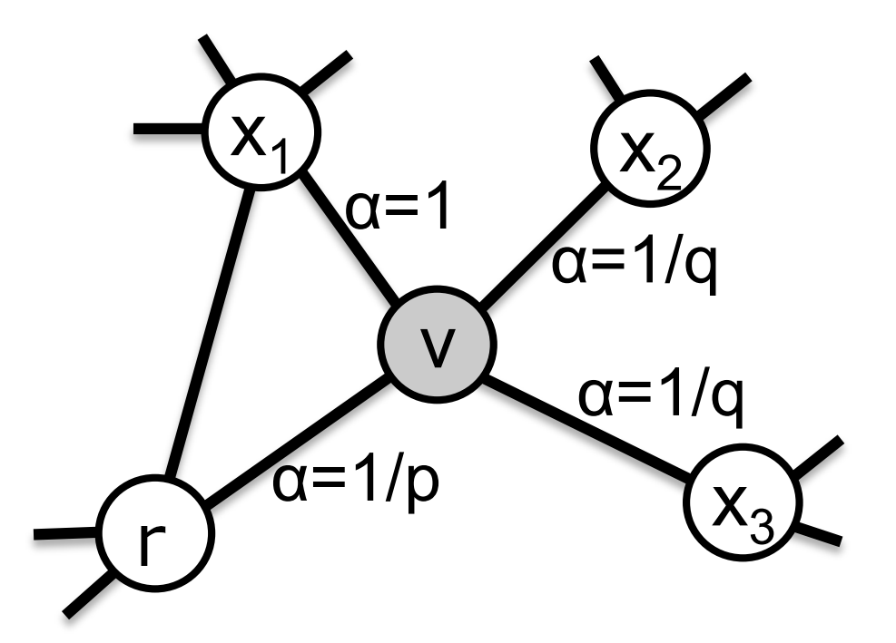
Figure 1: A step (at time $t$) of a $2^{nd}$ order random walk in a homogeneous graph presented in [10]. At time $t-1$ the random walk was in $X(t-1)=r$, and has just moved from node $r$ to node $v$ (image taken from [10]). Then, the probability of moving to any neighboring node is given by $\alpha w_{v,x}$, where $w_{v,x}$ is the edge weight, and $\alpha$ depends on a “return” parameter, $p$, and on an “outward” parameter $q$.

According to Leskovec (see Fig.1), this probability can be modeled by a (normalized) transition matrix $\Pi$ with elements:

$$\pi_{xvr}=\alpha_{p,q}w_{v,x}$$

where $w_{v,x}$ is the weight of the edge $(v,x)\in E$ and $\alpha_{p,q}$ is defined as:

$$\alpha_{p,q}=\left\{\begin{matrix}\frac{1}{p}\text{ if }d_{r,x}=0\\ \\ 1\text{ if }d_{r,x}=1\\ \\ \frac{1}{q}\text{ if }d_{r,x}=2\\ \end{matrix}\right.$$

where:

• $d_{r,x}$ is the “distance” from node $r$ to node $x$, that is the length of the shortest path from $r$ to $x$, whereby $d\in\{0,1,2\}$;

• $p$ is called the return (inward) hyper-parameter, and controls the likelihood of immediately revisiting a node in the walk;

• $q$ is the in-out hyper-parameter which controls the probability of exploring more distant parts of the graphs.

The advantage of this parametric "biased" RW is that by tuning $p$ and $q$ parameters we can both leverage the homophily (through a Depth-First Sampling (DFS)-like visit) and the structural (through a Breath-First Sampling (BFS)-like visit) characteristics of the graph under study. More precisely:

• setting $p<min(1,q)$ promotes the tendency of the $RW_{2}$ to backtrack a step, thus keeping the walk local by returning to the source node $r$;

• parameter $q$ allow us to simulate a DFS ($q<1$), thus capturing the homophily characteristics of the node, or a BFS ($q>1$), thus capturing the structural characteristics of the node.

3 Heterogeneous node2vec

Het-node2vec  introduces $2^{nd}$ order RWs that are node and edge type-aware, in the sense that the RW are biased according to the different types of nodes and edges in the graph. This is accomplished by introducing “switching” parameters that control the way the RW can move between different node and edge types, thus adding a further bias to the RW towards specific types of nodes and edges. From this standpoint our approach resembles the method proposed in [29], where “jumps” between different types of edges or nodes (inspired to Levy flights [11, 24, 4]) are stochastically run across an heterogeneous graph. Nevertheless, the authors focused on a different problem using a different algorithm: they proposed a first order random walk with restart in heterogeneous multi-graphs to predict node labels, while our approach performs biased second order random walks for graph representation learning purposes.

Het-node2vec adopts a sort of “attention” mechanism [30] in the world of RW, in the sense that RW samples are concentrated on the parts of the graph most important for the problem under investigation, while other less important parts received less attention, i.e. they are visited less intensely by the RW algorithm.

In this section we introduce three algorithms that extend node2vec to heterogeneous networks:

1. HeNHoE-2vec: Heterogeneous Nodes and Homogeneous Edges to vector

2. HoNHeE-2vec: Homogeneous Nodes and Heterogeneous Edges to vector

3. HeNHeE-2vec: Heterogeneous Nodes and Heterogeneous Edges to vector

The algorithms differ in the way the "biased" random walk is implemented, but share the common idea that the random walk can switch to nodes of different type (HeNHoE-2vec) or can switch to edges of different type (HoNHeE-2vec) or can switch to both nodes and edges of different type (HeNHeE-2vec).

In particular HoNHeE-2vec  and HeNHeE-2vec  can manage multigraphs, i.e. graphs characterized by multiple edges of different types between the same two nodes.

It is worth noting that HeNHoE-2vec  and HoNHeE-2vec  are special cases of HeNHeE-2vec.

3.1 Heterogeneous networks

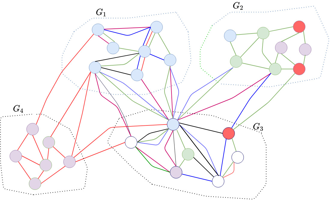
Figure 2: A heterogeneous multigraph with nodes and edges of different types. Different colors are used to represent node and edges types. Multiple types of edges may connect the same pair of nodes.

Fig. 2 represents a heterogeneous network with different types of nodes and edges. Different colours represent different node and edge types. The proposed algorithms are able to manage heterogeneous networks and multigraphs, i.e. graphs where the same pair of nodes may be connected by multiple types of edges. For didactic purposes, we show a graph with four different subgraphs in Figure 2 to illustrate the requirements for the three algorithms.

$G_{1}$ is a multigraph having nodes of the same type (cyan nodes) but edges of different types (edges having different colours) and multiple edges may connect the same pair of nodes: for this subgraph we can apply HoNHeE-2vec, since this algorithm can manage homogeneous nodes and heterogeneous edges.

$G_{2}$ is a graph having different types of nodes, but the same type of edges (green edges): for this subgraph we can apply HeNHoE-2vec, since this algorithm can manage heterogeneous nodes and homogeneous edges.

$G_{3}$ is a multigraph having both different types of nodes and edges, and the same pair of nodes may be connected by multiple edges: for this subgraph we can apply HeNHeE-2vec, since this algorithm can manage heterogeneous nodes and heterogeneous edges.

Finally $G_{4}$ is a graph with both homogeneous nodes and edges (violet nodes and red edges): for this subgraph the classical node2vec suffices, since this algorithm can be applied to graphs having homogeneous nodes and edges.

Note that the overall graph depicted in Fig. 2 can be managed with HeNHeE-2vec, since this algorithm generalizes both node2vec, HoNHeE-2vec  and HeNHoE-2vec.

3.2 HeNHoE-2vec. Heterogeneous Nodes Homogeneous Edges to vector algorithm

3.2.1 The algorithm

This algorithm extends node2vec by specifying the probabilities for the RW to switch between nodes with different types, adding the possibility to switch to another node $x_{o}$ having a type different from the source node $v_{s}$. One idea for the algorithm is that if we have a total of $n$ node types, we can either define the probability of switching between any two pairs of types, or we can define up to $n-2$ types as ’special’ and specify the probability of switching from a non-special node to a special node or vice versa, and analogously with edges. In most cases, we would define one category as ’special’.

More precisely, given a function that returns the type of each node $\phi:V\rightarrow\Sigma_{V}=\{V_{1},...,V_{N}\}$, where $V_{1},...,V_{N}$ represent different types of nodes, we may have a move from $v_{s}$ to $x_{o}$ such that $\phi(x_{o})\neq\phi(v_{s})$, using a switching parameter $s$ to modulate the probability to move toward a heterogeneous node. Note that the subscript s stands for same type of the source node $v_{s}$, while o stands for other type (see Fig. 3). More precisely we have:

• $r_{s}$ or $r_{o}$: the node visited before $v_{s}$ (preceding node) having ($r_{s}$) the same type as $v_{s}$, i.e. $\phi(r_{s})=\phi(v_{s})$, or a different type ($r_{o}$), i.e. $\phi(r_{o})\neq\phi(v_{s})$;

• $x_{s}$: the nodes in the neighborhood of $v_{s}$ and having same type as $v_{s}$: $\phi(x_{s})=\phi(v_{s})$;

• $x_{o}$: the nodes in the neighborhood of $v_{s}$ having type different from $v_{s}$: $\phi(x_{o})\neq\phi(v_{s})$.

The transition matrix used to decide where to “move” next is computed by introducing a “switch” parameter $s$, used in the calculation of $\alpha_{p,q,s}$:

$$P(X(t+1)=x|X(t)=v,X(t-1)=r)=\pi_{xvr}=\alpha_{p,q,s}w_{v,x}$$ (2)

$$\alpha_{p,q,s}=\left\{\begin{matrix}\text{if }\phi(v)=\phi(x):\hskip 14.22636pt\left\{\begin{matrix}\alpha=\frac{1}{p}\text{ if }d_{r,x}=0\\ \\ \alpha=1\text{ if }d_{r,x}=1\\ \\ \alpha=\frac{1}{q}\text{ if }d_{r,x}=2\\ \end{matrix}\right.\\ \\ \text{else }:\hskip 59.75095pt\left\{\begin{matrix}\alpha=\frac{1}{ps}\text{ if }d_{r,x}=0\\ \\ \alpha=\frac{1}{s}\text{ if }d_{r,x}=1\\ \\ \alpha=\frac{1}{qs}\text{ if }d_{r,x}=2\\ \end{matrix}\right.\\ \end{matrix}\right.$$ (3)

Eq. 3 shows an implementation of a $2^{nd}$ order RW for both the situations in which: a) at step $t+1$ we move to a node having the same type of $v_{s}$ ($\phi(v)=\phi(x)$); b) at step $t+1$ we move toward a node having a different type ($\phi(v)\neq\phi(x)$).

To better understand the dynamic of a $2^{nd}$ order RW in a heterogeneous network we consider two distinct cases (Fig. 3):

1. At step $t-1$ we start from a node of the same type of $X(t)=v_{s}$, and hence $X(t-1)=r_{s}$;

2. At step $t-1$ we start from a node having type different from $X(t)=v_{s}$, i.e. $X(t-1)=r_{o}$

These two cases in a $2^{nd}$ order RW are mutually exclusive in the sense that obviously for a fixed $t$ we may have either $X(t-1)=r_{s}$ or $X(t-1)=r_{o}$

The first case ($X(t-1)=r_{s}$) is depicted in Fig. 3 (A). When walking in the homogeneous graph which $v_{s}$ belong to, the $\alpha$ originally defined in [10] are used to weight edges toward $x_{s}$; when we move to another type of node, all the corresponding edges starting from $v_{s}$ are weighted through the switching parameter $s$ (eq. 3).

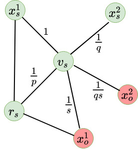
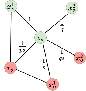
(A)	(B)

Figure 3: HeNHoE-2vec  $2^{nd}$ order $RW$. (A) starting from $X(t-1)=r_{s}$; (B) starting from $X(t-1)=r_{o}$. Green nodes are those having the same type of $X(t)=v_{s}$, while pink nodes are those have different type from $v_{s}$, i.e. “switch” nodes. On the edges the corresponding values of $\alpha_{p,q,s}$ are reported.

The second case ($X(t-1)=r_{o}$) is depicted in Fig. 3 (B). In this situation the node visited at step $t-1$ has a type different from that of $v_{s}$: for instance node $X(t-1)=r_{o}$ is a pink node while node node $X(t-1)=v_{s}$ is green, and the $\alpha_{p,q,s}$ values vary according to eq. 3).

The general idea of the proposed approach is to use the classical node2vec when moving inside a node homogeneous sub-graph; however, we consider the possibility to switch to other sub-graphs having different type of nodes, based on the value of an additional switching hyper-parameter $s$.

Essentially, if $s<1$, a switch between heterogeneous sub-graphs is encouraged. Moreover if $q<1$ Depth-First-Search sampling (DFS) is encouraged, where consecutively sampled nodes tend to have an increasing distance from the starting node.

Conversely, if $s>1$, switches are discouraged and the $RW$ tends to more cautiously stay in the same homogeneous graph. This especially happens when also $q>1$, encouraging a Breadth-First visit.

Summarizing, with respect to the original node2vec setting, that considers the interplay between the parameter $q$ that controls the depth-first or breadth-first like steps, and the $p$ “return” parameter that controls the probability of returning to the previous node, HeNHoE-2vec  introduces the novel $s$ “switching” parameter that allows us a node type-aware RW across the graph.

3.2.2 Simple, Multiple and Special node switching.

A single new parameter $s$ allows us to maintain the memory about the diversity of types between the preceding node and the node where to move. We name this modality of switching between different types of nodes as simple switching. Nevertheless note that, using only one $s$ parameter for all the switches between different node types, we loose the specificity of switching between two specific types of nodes of the overall heterogeneous network.

Multiple switching

To overcome this problem we can introduce different $s_{ij}$ for each switch from type $V_{i}$ to type $V_{j}$ (and viceversa). This approach, that we name multiple switching can introduce more control on the specificity of the switching process, but at the expenses of a major complexity of the resulting model. Indeed if we have $n$ different types of nodes we can introduce till to $\binom{n}{2}=\mathcal{O}(n^{2})$ different node switching parameters.

Special node switching

To avoid the complexity induced by multiple switching parameters, and to focus on specific node types, we can define a subset of the $n$ node types as special and we could simply specify the probability of switching from a non-special node to a special node or vice versa. This can be easily accomplished by relabeling the node types included in the special set as “special” and those not included as “non special”: in this way we can bring back to the simple switching algorithm (eq. 3) with only two types of nodes defined.

It is easy to see that this special node switching is a special case of the multiple switching: for instance if we have four node types and $V_{1}$ nodes are special and the other ones non special, we can set $s_{12}=s_{13}=s_{14}=c$, and by setting $c<1$ we can focus on switching to node of type $V_{1}$.

3.2.3 Versus specific switching

We note that we have considered only undirected edges. With an edge $(x,y)$ and $\phi(x)\neq\phi(y)$, say $x\in V_{1}$, and $y\in V_{2}$, we have the same switching parameter $s$ or $s_{12}$ when both moving from $x$ to $y$ and from $y$ to $x$. This is fine, but in this way we cannot capture the versus specific switching. For instance, if we would like to focus on $V_{1}$ nodes and we are in $y\in V_{2}$, by setting $s<<1$ we improve the probability to switch to $x\in V_{1}$. But if the neighbours of $x$ are nodes of type $V_{1}$, it is likely that at the next step we will come back to $y$. In this way we cannot specifically focus the RW on nodes of type $V_{1}$. To overcome this problem we could define different switching values $s_{12}\neq s_{21}$, thus modeling in different way the switch from $V_{1}$ to $V_{2}$ ($s_{12}$) with respect to the switch from $V_{2}$ to $V_{1}$ ($s_{21}$). This approach could be also applied to special nodes, by setting two different switching parameters for moving from special to non special and from non special to special nodes.

By using versus-specific switching we can obtain node embeddings more biased toward a specific type of nodes. For instance if we have $\Sigma_{V}=\{V_{1},V_{2}\}$, that is two types of nodes, by setting $s_{12}<s_{2,1}$ we improve the probability of switching to a node of type $V_{2}$. Indeed, for any $v,x,r\in V$ s.t. $\phi(v)=V_{1}$ and $\phi(x)=V_{2}$, with $(v,x),(r,v)\in E$, it is easy to see that the following property holds:

$$s_{12}<s_{21}\Longrightarrow\pi_{xvr}>\pi_{vxr}$$ (4)

that is it is more likely to move from a node labeled with $V_{1}$ towrard a node labeled with $V_{2}$ than viceversa. In this way we can focus on nodes labeled with $V_{2}$, thus introducing a sort of “attention bias” toward embeddings of nodes belonging to class $V_{2}$.

3.2.4 Computing transition probabilities

The value for the hyper-parameter $s$ (or $s_{i,j}$) should be “tuned” in order to obtain “good” node/edge embeddings, that is embeddings exploiting the topology of the overall heterogeneous network. This could be done by Bayesian optimization/grid search/random search. If we set $s<1$ or $s>1$ we can respectively encourage or discourage the visit of different types of nodes- On the contrary, by setting $s=1$ we in practice transform a heterogeneous network to a homogeneous one, and eq. 3 reduces itself to the original $2^{nd}$ order random walk of the Leskovec’s node2vec. Moreover if we set $p=1$ and $q=1$ we obtain a $1^{st}$ order random walk. If we finally set $s=p=q=1$ we obtain a $1^{st}$ order random walk in a homogeneous network, since we treat nodes in the same way without considering their different types.

We may have at most six different $\alpha_{p,q,s}$ values associated to the edges that connect $X(t)=v_{s}$ to either nodes of the same type or nodes of different type of $v_{s}$, namely $X(t+1)=x$, coming either from a node $X(t-1)=r_{s}$ or $X(t-1)=r_{o}$.

These $\alpha$ values are used to compute the unnormalized transition probability matrix $\Pi$ associated with the heterogeneous network. For instance, looking at Fig. 3, the unnormalized probability of moving from $v_{s}$ to the node $x_{s}^{2}$ of the same black subgraph is:

$$P\big{(}X(t+1)=x_{s}^{2}|X(t)=v_{s},X(t-1)=r_{o}\big{)}= \pi_{x_{s}^{2}v_{s}r_{o}}=\alpha_{pqs}w_{v_{s}x_{s}^{2}}=\frac{1}{q}w_{v_{s}x_{s}^{2}}$$

As another example, the unnormalized probability of moving from $v_{s}$ to a node $x_{o}^{2}$ belonging to a different subgraph is:

$$P\big{(}X(t+1)=x_{o}^{2}|X(t)=v_{s},X(t-1)=r_{o}\big{)}= \pi_{x_{o}^{2}v_{s}r_{o}}=\alpha_{pqs}w_{v_{s}x_{o}^{2}}=\frac{1}{qs}w_{v_{s}x_{o}^{2}}$$

As a final example, the unnormalized probability of coming back to node $r_{o}$ is:

$$P\big{(}X(t+1)=r_{o}|X(t)=v_{s},X(t-1)=r_{o}\big{)}= \pi_{r_{o}v_{s}r_{o}}=\alpha_{pqs}w_{v_{s}r_{o}}=\frac{1}{ps}w_{v_{s}r_{o}}$$

To normalize the transition probabilities $\pi$ to normalized probabilities $\hat{\pi}$, we can divide the unnormalized transition probabilities for the sum of the unnormalized ones connecting $v_{s}$ to its neighbours $N(v_{s})$:

$$\hat{\pi}_{xv_{s}r}=\sum_{v\in N(v_{s})}\frac{\pi_{xv_{s}r}}{\pi_{vv_{s}r}}$$

3.3 HoNHeE-2vec. Homogeneous Nodes Heterogeneous Edges to vector algorithm

3.3.1 The algorithm

This algorithm explicitly considers multigraphs, and can be applied to graphs with homogeneous nodes and heterogeneous edges, including edges of different types between the the same two nodes.

We can define a function $\psi:E\rightarrow\Sigma_{E}$, where $\Sigma_{E}$ represent different edge types.

We say that we have an “edge switch” in a $2^{nd}$ order random walk when, having $X(t-1)=r$, $X(t)=v$, $X(t+1)=x$, the edge $(r,v)$ has different type than $(v,x)$, i.e. $\psi(r,v)\neq\psi(v,x)$.

Looking at Fig. 4, to model the $2^{nd}$ order transition probabilities of moving from $v$ to one of its neighbouring nodes $x$, i.e.

$$P(X(t+1)=x|X(t)=v,X(t-1)=r)=\pi_{vxr}=\beta_{pqe}w_{vx}$$ (5)

where $w_{vx}$ is the weight of the edge $(v,x)$, we need to define the coefficient $\beta_{p,q,e}$ that biases the RW according to the three parameters $<p,q,e>$. Basically the algorithm is similar to HeNHoE-2vec, but this time a new parameter $e$ controls the probability of “edge switching” instead of “node switching” and can model the multigraph case with homogeneous nodes.

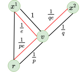
Figure 4: $2^{nd}$ order $RW$ according to the HoNHeE-2vec  algorithm. The node $v$ represents the node visited at step $t$, while $r$ the node visited at step $t-1$. Red edges represent switching edges. The weights over the edges represent the $\beta_{p,q,e}$ values according to eq. 7.

3.3.2 Computing transition probabilities

In Fig. 4 red edges refer to an edge switch, i.e. $\psi(r,v)\neq\psi(v,x)$, and the corresponding values of $\beta$ are shown. Depending on the distance of the node $x$ from $r$ and on the possible "switch" to another type of edge, we may have six different values of $\beta$ and of the resulting unnormalized transition probabilities $\pi_{v,x}$(see Fig. 4):

$$P\big{(}X(t+1)=r,\psi(r,v)=\psi(v,r)|X(t)=v,X(t-1)=r\big{)}=\pi_{rvr} = \frac{1}{p}w_{vr}$$

$$P\big{(}X(t+1)=r,\psi(r,v)\neq\psi(v,r)|X(t)=v,X(t-1)=r\big{)}=\pi_{(rv)r} = \frac{1}{pe}w_{vr}$$

$$P\big{(}X(t+1)=x^{1},\psi(r,v)=\psi(v,x^{1})|X(t)=v,X(t-1)=r\big{)}=\pi_{x^{1}vr} = w_{vx^{1}}$$

$$P\big{(}X(t+1)=x^{1},\psi(r,v)\neq\psi(v,x^{1})|X(t)=v,X(t-1)=r\big{)}=\pi_{(x^{1}v)r} = \frac{1}{e}w_{vx^{1}}$$

$$P\big{(}X(t+1)=x^{2},\psi(r,v)=\psi(v,x^{2})|X(t)=v,X(t-1)=r\big{)}=\pi_{x^{2}vr} = \frac{1}{q}w_{vx^{2}}$$

$$P\big{(}X(t+1)=x^{2},\psi(r,v)\neq\psi(v,x^{2})|X(t)=v,X(t-1)=r\big{)}=\pi_{(x^{2}v)r} = \frac{1}{qe}w_{vx^{2}}$$

The notation $\pi_{(vx)}$ using round brackets around the edge $(v,x)$ indicates that in the step from $v$ to $x$ an edge switch has occurred.

Summarizing, considering a network with homogeneous nodes and heterogeneous edges $G=(V,E,\psi)$, with $\psi:E\rightarrow\Sigma_{E}$, then the $2^{nd}$ order transition probabilities:

$$P\left(X(t+1)=x|X(t)=v,X(t-1)=r\right)=\pi_{vxr}=\beta_{pqe}w_{vx}$$

where $e$ is the "edge switching" parameter, can be modeled by computing $\beta_{pqe}$ in the following way:

$$\beta_{p,q,e}=\left\{\begin{matrix}\text{if }\psi(r,v)=\psi(v,x):\hskip 14.22636pt\left\{\begin{matrix}\beta=\frac{1}{p}\text{ if }d_{r,x}=0\\ \beta=1\text{ if }d_{r,x}=1\\ \\ \beta=\frac{1}{q}\text{ if }d_{r,x}=2\\ \end{matrix}\right.\\ \\ \text{else }:\hskip 76.82234pt\left\{\begin{matrix}\beta=\frac{1}{pe}\text{ if }d_{r,x}=0\\ \\ \beta=\frac{1}{e}\text{ if }d_{r,x}=1\\ \\ \beta=\frac{1}{qe}\text{ if }d_{r,x}=2\\ \end{matrix}\right.\\ \end{matrix}\right.$$ (7)

3.3.3 Characteristics of the algorithm

In eq. 7 the "if $\psi(r,v)=\psi(v,x)$" branch manages a $2^{nd}$ order RW when no edge switch is performed: in practice this is the classical node2vec algorithm. The else branch manages the switch to another type of edge instead, i.e. the case when $\psi(r,v)\neq\psi(v,x)$.

The $e>0$ parameter controls the probability of “switching” between two different types of edges: low values of $e$ improve the probability to switch in the random walk from ad edge of a given type to an edge of a different type.

By setting $e=1$, we treat the heterogeneous edges as homogeneous and in practice we reduce the algorithm to the classical node2vec.  The meaning of the $p$ and $q$ parameter is the same of node2vec.

Analogously to HeNHoE-2vec, we may introduce multiple $e$ parameters, one for each pair of types of edges, to model switches from a specific type of edge to another specific type. This can introduce more control in the biased random walk, but at the expenses of a more complex model.

To reduce complexity and to focus on on specific edge types, we can subdivide the in “special” and “non special”, as just discussed for the case of heterogeneous nodes (Section 3.2.2)

This algorithm can be applied to the synthetic lethality link prediction problem [20], when we have homogeneous nodes and heterogeneous edges. In this use case, we would define SLI edges as ’special’.

3.4 HeNHeE-2vec. Heterogeneous Nodes Heterogeneous Edges to vector algorithm

3.4.1 The algorithm

This algorithm can be applied to multigraphs $G=(V,E,\phi,\psi)$ with $\phi:V\rightarrow\Sigma_{V}$ and $\psi:E\rightarrow\Sigma_{E}$ having different types of nodes and edges.

The general idea behind this algorithm is to allow us to “switch” between both different types of nods (as in the HeNHoE-2vec), and also between different types of edges (as in the HoNHeE-2vec). To this end we need $4$ parameters, i.e. $p,q$, the original node2vec parameters that control BFS and DFS-like visit of the graph and the probability to come back to the previous node $X(t-1)$, and two additional parameters $s$ and $e$ that control the probability to switch respectively to another type of node or edge.

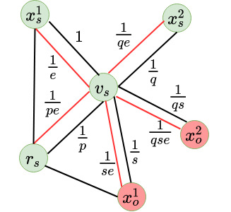
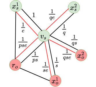
(A)	(B)

Figure 5: $2^{nd}$ order $RW$ according to the HeNHeE-2vec  algorithm. The node $v_{s}$ represents the node visited at step $t$. Red edges represent switching edges. The weights over the edges represent the $\gamma_{p,q,s,e}$ values according to eq. 7. (A) RW starting at $X(t-1)=r_{s}$, where nodes $r_{s}$ and $v_{s}$ share the same type; (B) RW starting at $X(t-1)=r_{o}$, where nodes $r_{o}$ and $v_{s}$ have different types.

Looking at Fig. 5, $v_{s}$ represents the node visited by the RW at the first step of a $2^{nd}$ order RW, i.e. $X(t)=v_{s}$. For node visited at the previous step, there are two possibilities: we can start from a node $X(t-1)=r_{s}$ having the same type of $v_{s}$ (Fig. 5, Left), or from a node $X(t-1)=r_{o}$ having a different type of $v_{s}$ (Fig. 5, Right):

1. $X(t-1)=r_{s}$, , with $\phi(r_{s})=\phi(v_{s})$

2. $X(t-1)=r_{o}$, with $\phi(r_{o})\neq\phi(v_{s})$

At step $t+1$ we can move back from $v_{s}$ to $r_{s}$ if $X(t-1)=r_{s}$ or to $r_{o}$ if $X(t-1)=r_{o}$, or we can move to a a node $x$ of the same type of $v_{s}$ at distance $1$ ($x_{s}^{1}$) or at distance $2$ ($x_{s}^{2}$) from $r_{s}$ or $r_{o}$, or we can alternatively move to a node $x$ having different type of $v_{s}$, at distance distance $1$ ($x_{o}^{1}$) or at distance $2$ ($x_{o}^{2}$) from $r_{s}$ or $r_{o}$:

1. $X(t+1)=r_{s}$, with $\phi(r_{s})=\phi(v_{s})$

2. $X(t+1)=r_{o}$, with $\phi(r_{o})\neq\phi(v_{s})$

3. $X(t+1)=x_{s}^{1}$, with $\phi(x_{s}^{1})=\phi(v_{s})$

4. $X(t+1)=x_{s}^{2}$, with $\phi(x_{s}^{2})=\phi(v_{s})$

5. $X(t+1)=x_{o}^{1}$, with $\phi(x_{o}^{1})\neq\phi(v_{s})$

6. $X(t+1)=x_{o}^{2}$, with $\phi(x_{o}^{2})\neq\phi(v_{s})$

Hence, looking at Fig. 5, considering a network with heterogeneous nodes and heterogeneous edges $G=(V,E,\phi,\psi)$, with $\phi:V\rightarrow\Sigma_{V}$ and $\psi:E\rightarrow\Sigma_{E}$, the $2^{nd}$ order transition probabilities

$$P\left(X(t+1)=x|X(t)=v,X(t-1)=r\right)=\pi_{xvr}=\gamma_{pqse}w_{vx}$$

where $s$ is the "node switching" and $e$ the "edge switching" parameters, can be modeled by computing $\gamma_{pqse}$ through the HeNHeE-2vec  algorithm:

$$\gamma_{pqse}=\left\{\begin{matrix}\text{if }\psi(r,v_{s})=\psi(v_{s},x):\hskip 14.22636pt\left\{\begin{matrix}\text{if }\phi(x)=\phi(v_{s}):\hskip 14.22636pt\left\{\begin{matrix}\gamma=\frac{1}{p}\text{ if }d_{r,x}=0\\ \gamma=1\text{ if }d_{r,x}=1\\ \gamma=\frac{1}{q}\text{ if }d_{r,x}=2\\ \end{matrix}\right.\\ \\ \text{else }:\hskip 62.59596pt\left\{\begin{matrix}\gamma=\frac{1}{ps}\text{ if }d_{r,x}=0\\ \gamma=\frac{1}{s}\text{ if }d_{r,x}=1\\ \gamma=\frac{1}{qs}\text{ if }d_{r,x}=2\\ \end{matrix}\right.\\ \\ \end{matrix}\right.\\ \\ \text{else }:\hskip 82.51282pt\left\{\begin{matrix}\text{if }\phi(x)=\phi(v_{s}):\hskip 14.22636pt\left\{\begin{matrix}\gamma=\frac{1}{pe}\text{ if }d_{r,x}=0\\ \gamma=\frac{1}{e}\text{ if }d_{r,x}=1\\ \gamma=\frac{1}{qe}\text{ if }d_{r,x}=2\\ \end{matrix}\right.\\ \\ \text{else }:\hskip 62.59596pt\left\{\begin{matrix}\gamma=\frac{1}{pse}\text{ if }d_{r,x}=0\\ \gamma=\frac{1}{se}\text{ if }d_{r,x}=1\\ \gamma=\frac{1}{qse}\text{ if }d_{r,x}=2\\ \end{matrix}\right.\\ \\ \end{matrix}\right.\end{matrix}\right.$$ (8)

3.4.2 Characteristics of the algorithm

HeNHeE-2vec  is a general algorithm to perform $2^{nd}$ order RW in heterogeneous multigraphs, characterized by the following features:

• can be applied to multigraphs having multiple types of nodes and edges

• can explore the graph according to a continuum between a BFS and a DFS visit (by tuning the $q$ parameter)

• can control the probability of walking a step back to the original source node (by the $p$ parameter)

• can control the probability to switch to different types of nodes (by the $s$ parameter)

• can control the probability to switch to different types of edges (by the $e$ parameter)

HeNHeE-2vec  is a generalization of the the previously presented algorithms. Indeed:

• if we set $e=1$ we obtain HeNHoE-2vec.

• if we set $s=1$ we obtain HoNHeE-2vec.

• if we set $e=1$ and $s=1$ we obtain node2vec.

Analogously to HeNHoE-2vec  and HoNHeE-2vec, we may introduce multiple $s$ and $e$ switching parameters, one for each pair of different types of nodes and edges. This approach on the one hand allow us to better control the biased RW, but on the other hand introduces a more complex model, with a large number of parameters to be tuned. Also in this case, analogously to Section 3.2.2, we can introduce “special” nodes and edges.

The algorithm is inherently parallel since we can generate multiple samples of $2^{nd}$ order RW in general heterogeneous networks starting at the same time from each node of the graph.

The complexity of a single $2^{nd}$ order RW step for single node of the graph is $\mathcal{O}(1)$. To perform one step for each node of the graph, the complexity is $\mathcal{O}(n)$ with $n=|V|$. To perform a random walk of length $k$, the complexity is $\mathcal{O}(kn)$, and to perform $m$ RW of length $k$ for each node the complexity is $\mathcal{O}(kmn)$. If $km<<n$ then the complexity is $\mathcal{O}(n)$, and if $km\simeq n$, then the complexity is $\mathcal{O}(n^{2})$.

As an example of possible relevant applications of HeNHeE-2vec, we could consider the analysis of KG-COVID-19 [23], or the analysis of the heterogeneous Monarch network [26].

4 Conclusion

We proposed Het-node2vec an algorithmic framework to run biased $2^{nd}$ order random walks on heterogeneous networks, to obtain embeddings that are node and edge-type aware. The proposed approach can be viewed as an extension of the classical node2vec algorithm, since the random walk is further biased, according to the type of nodes and edges. This is accomplished through simple “switching” mechanisms, controlled by appropriated “switching parameters”, by which a random walk can stochastically move between different types of nodes and edges, and can focus on specific types of nodes and edges that are of particular interest for the specific learning problem under investigation. The algorithms are general enough to be applied to general unsupervised and supervised problems involving graph representation learning, ranging from edge and node label prediction to graph clustering, considering different possible application domains, ranging from biology and medicine to economy, social sciences and more in general for the analysis of complex heterogeneous systems.

References

- [1] Dzmitry Bahdanau, Kyunghyun Cho, and Yoshua Bengio. Neural machine translation by jointly learning to align and translate. In Yoshua Bengio and Yann LeCun, editors, 3rd International Conference on Learning Representations, ICLR 2015, San Diego, CA, USA, May 7-9, 2015, Conference Track Proceedings, 2015.
- [2] Shaosheng Cao, Wei Lu, and Qiongkai Xu. Deep neural networks for learning graph representations. In Proceedings of the Thirtieth AAAI Conference on Artificial Intelligence, AAAI’16, page 1145–1152. AAAI Press, 2016.
- [3] Chaochao Chen, Xinxing Yang, Jun Zhou, Xiaolong Li, and Le Song. Heterogeneous graph neural networks for malicious account detection. In Proc. of CIKM, pages 2077–2085, 10 2018.
- [4] Yuzhou Chen, Yulia R Gel, and Konstantin Avrachenkov. Lfgcn: Levitating over graphs with levy flights. arXiv preprint arXiv:2009.02365, 2020.
- [5] Yuanfei Dai, Shiping Wang, Neal N. Xiong, and Wenzhong Guo. A survey on knowledge graph embedding: Approaches, applications and benchmarks. Electronics, 9(5-750), 2020.
- [6] Yuxiao Dong, Nitesh V. Chawla, and Ananthram Swami. Metapath2vec: Scalable representation learning for heterogeneous networks. In Proceedings of the 23rd ACM SIGKDD International Conference on Knowledge Discovery and Data Mining, KDD ’17, page 135–144, New York, NY, USA, 2017. Association for Computing Machinery.
- [7] Yuxiao Dong, Ziniu Hu, Kuansan Wang, Yizhou Sun, and Jie Tang. Heterogeneous network representation learning. In Christian Bessiere, editor, Proceedings of the Twenty-Ninth International Joint Conference on Artificial Intelligence, IJCAI-20, pages 4861–4867. International Joint Conferences on Artificial Intelligence Organization, 7 2020. Survey track.
- [8] Charles C Fries. Meaning and linguistic analysis. Language, 30(1):57–68, 1954.
- [9] Justin Gilmer, Samuel S. Schoenholz, Patrick F. Riley, Oriol Vinyals, and George E. Dahl. Neural message passing for quantum chemistry. In Proceedings of the 34th International Conference on Machine Learning - Volume 70, ICML’17, page 1263–1272. JMLR.org, 2017.
- [10] Aditya Grover and Jure Leskovec. Node2vec: Scalable feature learning for networks. In Proceedings of the 22nd ACM SIGKDD International Conference on Knowledge Discovery and Data Mining, KDD ’16, page 855–864, New York, NY, USA, 2016. Association for Computing Machinery.
- [11] Quantong Guo, Emanuele Cozzo, Zhiming Zheng, and Yamir Moreno. Levy random walks on multiplex networks. Scientific reports, 6(1):1–11, 2016.
- [12] William L. Hamilton, Rex Ying, and Jure Leskovec. Inductive representation learning on large graphs. In Proceedings of the 31st International Conference on Neural Information Processing Systems, NIPS’17, page 1025–1035, Red Hook, NY, USA, 2017. Curran Associates Inc.
- [13] Zellig S Harris. Distributional structure. Word, 10(2-3):146–162, 1954.
- [14] Yu He, Yangqiu Song, Jianxin Li, Cheng Ji, Jian Peng, and Hao Peng. Hetespaceywalk: A heterogeneous spacey random walk for heterogeneous information network embedding. In Proceedings of the 28th ACM International Conference on Information and Knowledge Management, CIKM ’19, page 639–648, New York, NY, USA, 2019. Association for Computing Machinery.
- [15] Ziniu Hu, Yuxiao Dong, Kuansan Wang, and Yizhou Sun. Heterogeneous graph transformer. In Proceedings of The Web Conference 2020, WWW ’20, New York, NY, USA, 2020. Association for Computing Machinery.
- [16] Thomas Kipf and Max Welling. Semi-supervised classification with graph convolutional networks. In Proceedings of ICLR’17, 09 2017.
- [17] V. Martinez, F. Berzal, and JC Cubero. A survey of link prediction in complex networks. ACM Computing Surveys, 49(6), 2017.
- [18] Tomas Mikolov, Ilya Sutskever, Kai Chen, Greg Corrado, and Jeffrey Dean. Distributed representations of words and phrases and their compositionality. In Proceedings of the 26th International Conference on Neural Information Processing Systems - Volume 2, NIPS’13, page 3111–3119, Red Hook, NY, USA, 2013. Curran Associates Inc.
- [19] Nagarajan Natarajan and Inderjit S. Dhillon. Inductive matrix completion for predicting gene–disease associations. Bioinformatics, 30(12):i60–i68, 06 2014.
- [20] N. O’Neil, M. Bailey, and P. Hieter. Synthetic lethality and cancer. Nat Rev Genet, 18:613–623, 2017.
- [21] Chanyoung Park, Donghyun Kim, Qi Zhu, Jiawei Han, and Hwanjo Yu. Task-guided pair embedding in heterogeneous network. In Proceedings of the 28th ACM International Conference on Information and Knowledge Management, CIKM ’19, page 489–498, New York, NY, USA, 2019. Association for Computing Machinery.
- [22] Bryan Perozzi, Rami Al-Rfou, and Steven Skiena. Deepwalk: Online learning of social representations. In Proceedings of the 20th ACM SIGKDD International Conference on Knowledge Discovery and Data Mining, KDD ’14, page 701–710, New York, NY, USA, 2014. Association for Computing Machinery.
- [23] J Reese, U Deepak, T. Callahan, et al. Kg-covid-19: A framework to produce customized knowledge graphs for covid-19 response. Patterns, page 100155, 2021.
- [24] Alejandro P Riascos and José L Mateos. Long-range navigation on complex networks using lévy random walks. Physical Review E, 86(5):056110, 2012.
- [25] M. Schlichtkrull, T.N. Kipf, P. Bloem, vandenBerg R., I. Titov, and M. Welling. Modeling relational data with graph convolutional networks. In The Semantic Web. ESWC 2018, volume 10843 of Lecture Notes in Computer Science. Springer, 2018.
- [26] KA Shefchek, NL Harris, M Gargano, et al. The monarch initiative in 2019: an integrative data and analytic platform connecting phenotypes to genotypes across species. Nucleic Acids Res., 48(D1):D704–D715, 2020.
- [27] Jian Tang, Meng Qu, and Qiaozhu Mei. Pte: Predictive text embedding through large-scale heterogeneous text networks. In Proceedings of the 21th ACM SIGKDD International Conference on Knowledge Discovery and Data Mining, KDD ’15, page 1165–1174, New York, NY, USA, 2015. Association for Computing Machinery.
- [28] Jian Tang, Meng Qu, Mingzhe Wang, Ming Zhang, Jun Yan, and Qiaozhu Mei. Line: Large-scale information network embedding. In WWW ’15: Proceedings of the 24th International Conference on World Wide Web, WWW ’15, page 1067–1077, Republic and Canton of Geneva, CHE, 2015. International World Wide Web Conferences Steering Committee.
- [29] Alberto Valdeolivas, Laurent Tichit, Claire Navarro, Sophie Perrin, Gaelle Odelin, Nicolas Levy, Pierre Cau, Elisabeth Remy, and Anaïs Baudot. Random walk with restart on multiplex and heterogeneous biological networks. Bioinformatics, 35(3):497–505, 2019.
- [30] Petar Velickovic, Guillem Cucurull, A. Casanova, A. Romero, P. Liò, and Yoshua Bengio. Graph attention networks. ArXiv, abs/1710.10903, 2018.
- [31] H. Wang, J. Wang, J. Wang, M. Zhao, W. Zhang, F. Zhang, W. Li, X. Xie, and M. Guo. Learning graph representation with generative adversarial nets. IEEE Transactions on Knowledge and Data Engineering, pages 1–1, 2019.
- [32] Pengyang Wang, Jiawei Zhang, Guannan Liu, Yanjie Fu, and Charu Aggarwal. Ensemble-spotting: Ranking urban vibrancy via poi embedding with multi-view spatial graphs. In Proceedings of the 2018 SIAM International Conference on Data Mining (SDM), pages 351–359, 2018.
- [33] Xiao Wang, Peng Cui, Jing Wang, Jian Pei, Wenwu Zhu, and Shiqiang Yang. Community preserving network embedding. In Proceedings of the Thirty-First AAAI Conference on Artificial Intelligence, AAAI’17, page 203–209. AAAI Press, 2017.
- [34] Xiao Wang, Houye Ji, Chuan Shi, Bai Wang, Yanfang Ye, Peng Cui, and Philip S Yu. Heterogeneous graph attention network. In The World Wide Web Conference, WWW ’19, page 2022–2032, New York, NY, USA, 2019. Association for Computing Machinery.
- [35] Z. Wu, S. Pan, F. Chen, G. Long, C. Zhang, and P. S. Yu. A comprehensive survey on graph neural networks. IEEE Transactions on Neural Networks and Learning Systems, pages 1–21, 2020.
- [36] Y. Xie, B. Yu, S. Lv, C. Zhang, G. Wang, and M. Gong. A survey on heterogeneous network representation learning. Pattern Recognition, 116(107936), 2021.
- [37] Chuxu Zhang, Dongjin Song, Chao Huang, Ananthram Swami, and Nitesh V. Chawla. Heterogeneous graph neural network. In Proceedings of the 25th ACM SIGKDD International Conference on Knowledge Discovery and Data Mining, KDD ’19, page 793–803, New York, NY, USA, 2019. Association for Computing Machinery.
- [38] D. Zhang, J. Yin, X. Zhu, and C. Zhang. Homophily, structure, and content augmented network representation learning. In 2016 IEEE 16th International Conference on Data Mining (ICDM), pages 609–618, 2016.
- [39] D. Zhang, J. Yin, X. Zhu, and C. Zhang. Network representation learning: A survey. IEEE Transactions on Big Data, 6(1):3–28, 2020.
- [40] Marinka Zitnik, Monica Agrawal, and Jure Leskovec. Modeling polypharmacy side effects with graph convolutional networks. Bioinformatics, 34(13):i457–i466, 06 2018.
- [41] Marinka Zitnik and Jure Leskovec. Predicting multicellular function through multi-layer tissue networks. Bioinformatics, 33(14):i190–i198, 07 2017.