Compositeness, Bargmann-Wigner solutions within a U(1)-interaction quantum-field-theory expansion, and charge

Abstract

New solutions of the Bargmann-Wigner equations are obtained: free fermion-antifermion pairs, each satisfying Dirac’s equation, with parallel momenta and momenta on a plane, produce vectors satisfying Proca’s equations. These equations are consistent with Dirac’s and Maxwell’s equations, as zero-order conditions within a Lagrangian expansion for the U(1)-symmetry quantum field theory. Such vector solutions’ demand that they satisfy Maxwell’s equations and quantization fix the charge. The current equates the vector field, reproducing the superconductivity London equations, thus, binding and screening conditions. The derived vertex connects to QCD superconductivity and constrains four-fermion interaction composite models.

^∗ email: bespro@fisica.unam.mx

I Introduction

The Standard Model[1]-[3] (SM) accurately describes elementary particles and their hypercharge ($Y$), weak (left-handed, $L$) and color ($c$) interactions, defined by the gauge groups U(1)${}_{Y}\times$SU(2)${}_{L}\times$SU(3)_c, respectively; yet, puzzles remain as the origin of phenomenological constants, like the interactions’ coupling constants.

Insight on these was provided on proposed structures that generalize physical features: grand-unified theories[4] assume a common group for the interactions, requiring a unique coupling constant at the unification scale, and setting constraints on their values.

Compositeness, which refers to related properties in systems built from simpler ones, underlies many physical systems and provides information on them. The quark model[5] is one of its paradigms, as hadron features are derived from the quarks’. Likewise, theories with more fundamental elements were proposed to explain SM features[6, 7]; supersymmetry generalizes the SM composite quantum numbers to additional feasible fermions and bosons[8]; and SM structures can predict such constants[9, 10], all suggesting elementary composite configurations may provide clues, for which we review relevant physical and formal setups.

In superconductivity, compositeness is also present. For its Bardeen-Cooper-Schrieffer’s[11] (BCS) theory, the relevant degree of freedom is a Cooper pair conformed of an electron and a hole. In addition, interaction screening allows for free-particle behavior, which may enable elementary-particle properties to become manifest.

An early application of this scheme in particle physics[12] describes a mass-generating mechanism for fermions and composite bosons, relating their masses, through a hypothesised interaction built from four fermions, with binding and self-consistency features. A correspondence was argued between such a composite model and the U(1) theory[13]. The idea of a quark condensate generating the Higgs[14, 15], with a binding effect analogous to superconductivity, remains feasible. Such a mechanism is dynamical, as for radiative corrections[16].

We use the simpler Abelian U(1)-group gauge symmetry, relevant at all ranges. With focus on fundaments, a gauge-interaction quantum field theory is a useful framework as a four-vector’s spin-1 degree of freedom can be constructed in terms of two fermions’ spin-1/2. The U(1) interaction picks a particular four-fermion interaction as effective theory for the Nambu-Jona Lasinio model[17]; it comprises physically the hypercharge and the electromagnetic interactions, and an effective version for the strong interaction that, e. g., models the quark anti-quark potential[18].

Framed within the U(1) theory, the Bargmann-Wigner equations[19] depart from a fermion-antifermion pair, each element satisfying Dirac’s equation, that conforms a current element satisfying Proca’s, all comprising a composite configuration.

In this paper, we present a new class of Bargmann-Wigner solutions, which signifies their space is dimensionally larger. We show that these equations constitute zero-order terms, within a generated expansion for the Lagrangian, for a U(1)-interaction quantum field theory, constituting a compositeness limit. For such systems, we show that Maxwell’s equations and quantization fix the coupling constant. Such configurations satisfy superconductivity conditions through the London equations, connecting the current and the U(1) vector. Finally, we argue that this setup applies to QCD superconductivity, among other systems. The material is organized thus: Section II develops a Lagrangian expansion that contains the free Dirac’s and Maxwell’s equations as zero-order conditions; in Section III, these are connected to the Bargmann-Wigner equations, presenting more solutions. Section IV derives a charge from Maxwell’s equations consistency and quantization. Section V shows that the London’s equations are implied, linking fermion-antifermion states to superconductivity. Section VI analyzes other applications and draws conclusions. Appendixes A-F present calculations in detail; notably, Appendix B contains Bargmann-Wigner solutions with fermion-antifermion same-momentum and arbitrary spin configurations, and with combinations of momenta on the same plane, including a confined configuration. Appendix C presents the adapted Bargmann-Wigner equations used.

II U(1) expansion

A U(1)-symmetry imposes four-vector field $A_{\mu}(x)$ minimal substitution on Dirac’s equation[20], setting its interaction with the fermion represented by $\psi$, a four-complex column wave function accounting for spin and the antiparticle, with the U(1) four-current given by $gj_{\mu}=g\bar{\psi}\gamma_{\mu}\psi$, with coupling $g$. The $x$ space-time coordinate dependence is hence usually omitted. The U(1) Lagrangian ${\cal L}(A_{\mu},\psi)={\cal L}_{D}(\psi)+{\cal L}_{K}(A_{\mu})+{\cal L}_{I}(A_{\mu},j_{\mu})$ contains the free-Dirac ($D$), vector-kinetic ($K$) components and interaction term ($I$) ${\cal L}_{I}(A_{\mu},j_{\mu})=-gA_{\mu}j^{\mu}$. Defining the the lowest-order solution through an external c-number current[21] $j^{s}_{\mu}$ leads to

$${\cal L}_{C}(A_{\mu},\psi)={\cal L}(A_{\mu},\psi)-{\cal L}_{I}(A_{\mu},j^{\mu})+{\cal L}_{I}(A_{\mu},j_{\mu}^{s})={\cal L}_{D}(\psi)+{\cal L}_{K}(A_{\mu})+{\cal L}_{I}(A_{\mu},j_{\mu}^{s})$$ (1)

as zero-order term, with corrections ${\cal L}_{I}(A_{\mu},j_{\mu})-{\cal L}_{I}(A_{\mu},j_{\mu}^{s})$.

Next, we obtain the equations of motion to this order, showing that extended Bargmann-Wigner equations connect to them, allowing for a charge definition, and implying that $A_{\mu}$ satisfies the superconductivity[11] London’s equations. We shall use the relativistic-quantum-mechanics framework and the quantization/normalization condition.

III Dirac’s and Maxwell’s equations connection to Bargmann-Wigner equations

The Euler-Lagrange equations for ${\cal L}_{C}(A_{\mu},\psi)$ in Eq. 1 imply Dirac’s free-particle equation for a U(1)-charged fermion

$$(i\partial_{\mu}\gamma^{\mu}-m)\psi(x)=0,$$ (2)

with $m$ its mass, $\gamma_{\mu}$ 4$\times$4 matrices satisfying the Clifford algebra $\{\gamma_{\mu},\gamma_{\nu}\}=2Ig_{\mu\nu}$, transforming under the Lorentz group as vectors, $I$ the identity matrix, and $g_{\mu\nu}$ the metric. These matrices are given in the Dirac representation in Appendix A, with solutions in Appendix B.

Now, with the current notation ${j^{s}}^{\mu}\rightarrow j^{\mu}$, not specifying the zero order, variations of $\cal L_{C}$ over $A_{\mu}$ lead to Maxwell’s equations

$${\partial}^{\nu}({\partial}_{\nu}A^{s}_{\mu}-{\partial}_{\mu}A^{s}_{\nu})=4\pi gj_{\mu},$$ (3)

where $A^{s}_{\mu}$ provides the solution to Maxwell’s equations at this order. The homogenous equations are also implied for $F_{\mu\nu}={\partial}_{\mu}A^{s}_{\nu}-{\partial}_{\nu}{A^{s}}_{\mu}$

$$\frac{1}{2}\partial^{\mu}\epsilon_{\mu\nu\eta\sigma}{F}^{\eta\sigma}=0.$$ (4)

The Bargmann-Wigner[19] equations (applied for two quanta, Appendix C) comprise two identical spinors satisfying each Dirac’s equation 2. These conform a vector satisfying in turn Proca’s equations[22] (which generalize Maxwell’s equations to the massive case)

$$(\hbar c)^{2}[{\partial}^{\nu}({\partial}_{\mu}j_{\nu}-{\partial}_{\nu}j_{\mu})]=(2mc^{2})^{2}{j}_{\mu}.$$ (5)

The current is thus equated to its derivatives with an explicit Maxwell structure, and mass $2m$, as $\partial^{\mu}j_{\mu}=0$ (Lorentz gauge). These equations translate such spin-1/2 elements to non-diagonal current components, for an electron and a positron wave functions $j_{\mu}=\langle\psi_{c}|\gamma_{0}\gamma_{\mu}|\psi\rangle$, where $\psi_{c}=C\gamma_{0}\psi^{*}$, $C=i\gamma^{2}\gamma^{0}$ is the charge-conjugation matrix in the Dirac representation, for relevant cases (Appendix C). Fig. 1 represents these solutions, reinterpreted as a fermion-antifermion pair, as they connect to states in a Feynman diagram in which it converts to a massive vector. Given the antisymmetric form $F^{j}_{\mu\nu}={\partial}_{\mu}j_{\nu}-{\partial}_{\nu}j_{\mu}$, Maxwell’s homogeneous equations are satisfied, as in Eq. 4. Same-momentum opposite spin, and arbitrary energy, spin, and momentum on a plane, extend the basis for larger kinematical regions, implying a feasible description of more than one fermion-antifermion pair (Appendix C). For the fermion self-energy, the U(1) theory leads to an effective (four-fermion) Hartree interaction, which connects to the contact vector-vector term in ${\cal L}_{I}(A_{\mu},j_{\mu}^{s})$, constituting an interaction case in the Nambu-Jona Lasinio model[17].

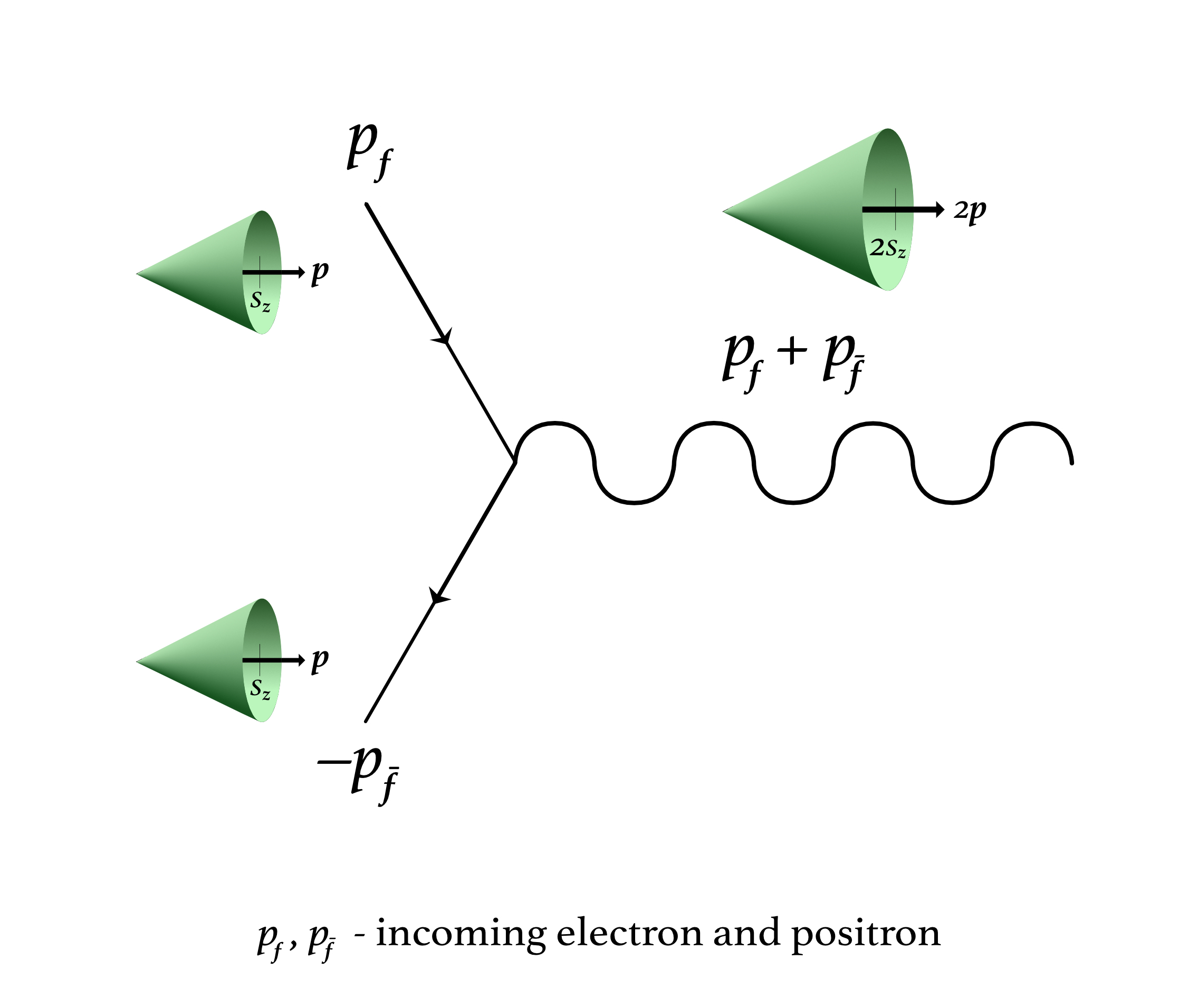
Figure 1: Feynman diagram with vertex $ig\gamma_{\mu}$, related to solutions at fixed volume $V$, as described in Eq. 3. Incoming fermion-antifermion $f$-$\bar{f}$ have four-momenta $p_{f}$, $p_{\bar{f}}$. The Bargmann-Wigner solutions here have parallel momenta with $p_{f}=p_{\bar{f}}=(E,0,0,p_{z})$, energy $E=\sqrt{m^{2}+|{\bf p}|^{2}}$, ${\bf p}=(0,0,p_{z})$, each with spin $s_{z}$, represented by the small cones, producing massive vector $A^{s}_{\mu}$ with four-momentum $p_{f}+p_{\bar{f}}$, polarization $2s_{z}$. The inverse process represents vector-particle annihilation into two fermions.

For the field $A^{s}_{\mu}$ in Maxwell’s equations 3, generated by $j_{\mu}$, the equations in 5 are a necessary consistency condition restricting $g$. With their common element $j_{\mu}$ on the right-hand side, matching these equations implies the former is the latter times $4\pi g/(2mc^{2})^{2}$. We rewrite Eq. 5 in terms of

$$A^{\psi}_{\mu}=\frac{(\hbar c)^{2}}{(2mc^{2})^{2}}\bar{\psi}\gamma_{\mu}\psi.$$ (6)

Using the Lorentz-gauge condition

$${\square}A^{\psi}_{\mu}=-\bar{\psi}\gamma_{\mu}\psi,$$ (7)

where the ${\square}=\partial^{\mu}\partial_{\mu}$ is the d’Alambertian. Comparing the same elements, with derivatives acting upon them, leads to

$$4\pi gA^{\psi}_{\mu}=-A^{s}_{\mu}.$$ (8)

This equation ascertains $A^{\psi}_{\mu}$ is the charge-independent component.

IV Vector quantization and the U(1) charge

Quantum field theory imposes field quantization, which identifies the factor connecting $A^{\psi}_{\mu}$ with $A^{s}_{\mu}$ in Eq. 6, as they constitute the same quantum. We require the normalization condition on conserved quantities as a proxy to quantization rules for vectors[23].

A vector component extended to be massive, is analyzed in Appendix D. The Maxwell’s energy-quantization condition[23, 24], for Eq. 3, for such a vector with momentum $2{\bf p}$, and mass $2m$, is

$$\int d^{3}x\frac{1}{4\pi}[\frac{1}{2}(|{\bf E}^{s}|^{2}+|{\bf B}^{s}|^{2})+\frac{(2m)^{2}}{2}(2{A^{s}}_{0}{A^{s}}_{0}-g_{00}{A^{s}}_{\mu}{A^{s}}^{\mu})]=2E,$$ (9)

where $E=\sqrt{(mc^{2})^{2}+|c\bf p|^{2}}$, and we define the electric and magnetic components from ${A^{s}}^{\mu}=({A^{0}}^{s},{\bf A}^{s})$

$${\bf E}^{s} = -\partial^{0}{{\bf A}^{s}}-{\mbox{\boldmath$\nabla$\unboldmath}}{A^{0}}^{s}$$ (10)

$${\bf B}^{s} = {\mbox{\boldmath$\nabla$\unboldmath}}\times{\bf A}^{s},$$

valid for a U(1) complex field, in correspondence with the Klein-Gordon equation case.

On the other hand, a Proca positive-energy free field with the same four-momentum quantum-mechanical normalization in Eq. 7 requires[25]

$$-\int d^{3}x{A^{\psi}_{\mu}}^{*}\frac{i}{2c}\overleftrightarrow{\partial}^{0}{A^{\psi}}^{\mu}=1.$$ (11)

This massive-vector quantization condition and that of the U(1) field connection in Eq. 9 implies, comparing their normalization constants (Appendixes B, D)

$$\sqrt{4\pi\hbar c}A^{\psi}_{\mu}=-A^{s}_{\mu}.$$ (12)

Combining this equation and the Dirac and U(1) vector relation in Eq. 8 fixes $g$:

$$g/\sqrt{\hbar c}=1/\sqrt{4\pi},$$ (13)

whose value is $g_{eLH}/\sqrt{\hbar c}=\sqrt{4\pi}g/\sqrt{\hbar c}=1$ in Lorentz-Heaviside units.

The conserved property of the constructed energy and probability in Eqs. 9, 11, respectively, ensure that $g$ is Lorentz and gauge invariant. The obtained value, $\alpha_{g}^{-1}=\hbar c/g^{2}=4\pi\simeq 12.6$, is between the couplings[26]: weak $g_{w}$, hypercharge $g^{\prime}$ and strong $g_{s}$ (associated to its U(1) effective form[27]) at low energies, consistently with unification conditions. Links to SM interactions are feasible, through a unification model. The unification coupling constrains SM ones, as obtained in other theories and energy scales[4, 28]. One connection is through quantum chromodynamics, for its asymptotically-free behaviour[29] relates to a unification energy scale, with $g$ interpreted as the effective U(1) component[27] sets $(4/3)g_{s}^{2}=g^{2}$, implying $\alpha_{g_{s}}^{-1}=\frac{16\pi}{3}\simeq 16.76$ . Such values are consistent with the unified coupling constant in some models[30], with emphasis on those with compositeness[31]. A generic U(1) interaction with stationary coupling running up to the unification scale, within feasible models[32] accounts for such scales at high-energy. Such a value is also consistent with compositeness theories under fixed-point conditions for the coupling[15].

V Fermion-antifermion self-superconductor

The Maxwell’s equations also relate the current to the vector potential. Using Eqs. 6, 8, and 13, extended London’s equations are obtained

$$j_{\mu}=-\frac{g\left(\frac{2mc}{\hbar}\right)^{3}A^{s}_{\mu}}{2mc},$$ (14)

as $A^{s}_{\mu}$ reproduces superconductivity behavior. Paired particles with $2m$ mass associate this superconductivity condition to the density $n_{j}=\left(\frac{2mc}{\hbar}\right)^{3},$ with cube unit size of reduced Compton wavelength[33] $\lambda_{C}=\frac{\hbar}{2mc}$. We compare them using the generalized Gordon identity[34] (Appendix F) for the interactive case

$$\bar{\psi}i\overleftrightarrow{\partial}_{\mu}\psi-2g\bar{\psi}\psi A_{\mu}+\frac{i}{2}{\partial}^{\nu}\bar{\psi}[\gamma_{\mu},\gamma_{\nu}]\psi=2m\bar{\psi}\gamma_{\mu}\psi.$$ (15)

Such identities contain the Bargmann-Wigner equations in the compositeness limit. With proper normalization and multiplying by $g$, the U(1) four-current $gj_{\mu}=g\bar{\psi}\gamma_{\mu}\psi$ has[11], on the left-hand side, a paramagnetic contribution (first term), and a diamagnetic (second) term, where ${\bf A}(x)$ is the U(1) vector potential, reproducing for the current the structure of London’s superconductivity equations[35] (in the London gauge ${\mbox{\boldmath$\nabla$\unboldmath}}\cdot{\bf A}=0$)

$$g{\bf j}(x)=-\frac{{g}^{2}{\bf A}(x)n_{c}}{mc},$$ (16)

where $n_{c}$ is the electron density, to be compared with the local scalar bilinear $\bar{\psi}\psi$. Eq. 16 is a valid approximation to Eq. 15 with only the second term on the left-hand side, in the regime of small wave-function variation, e. g., $|\bar{\psi}i\overleftrightarrow{\partial}_{\mu}\psi/\bar{\psi}\psi|\ll|2gA_{\mu}|$. For this second superconducting component in Eq. 15, the U(1) field is associated to the system’s length $L$. Over long distances $L\gg\lambda_{C}$, such component’s contribution is negligible as compared to the third component, which contains the Maxwell’s equations contribution in Eq. 5, (Appendix F) and depends on $\lambda_{C}$, implying this constitutes a sizable component in a fermion’s generated interactive field. As for the Meissner effect, a current is generated without friction, as a classical expansion of this equation manifests it. Unlike the usual London equations, which describe current under external fields, here they are self-consistent; also, the current oscillates, not decays. Substitution of Eq. 15 into ${\cal L}_{I}(A_{\mu},j_{\mu}^{s})$ implies such a term is atractive, as the on-shell $A_{\mu}$ (Appendix D) is space-like.

This scheme applies to models and scenarios in which compositeness is assumed explicitly, starting with the application of the BCS model within quantum field theory through the Nambu Jona-Lasinio model[12]; SM extensions reproduce spontaneous symmetric breaking[14, 15] through quark condensates, with supersymmetry[36], technicolor[37], and some unification models.

VI Applications and conclusions

Methods are added to known cases as extensions [28, 37] requiring composite elements. Compositeness can be applied to SM couplings[9], as connections were recently exploited to obtain information on the quark masses[10]. As the current is a particular bilinear-spinor term, similarly to superconductor Cooper pairs[38], a composite regime is feasible, under some conditions. Generically, a 4-fermion interaction is self-consistent, as described in the Hartree approximation[39] or as order parameter in the Landau-Ginzburg theory[40]. The generation of a boson quantum within superconducty[11, 12] suggests screening and binding conditions.

The consistency of the implied Bargmann-Wigner condition in Eq. 5 with Maxwell’s equations and quantization fixes the effective U(1) charge. Derived London’s equations imply superconductivity conditions, as a zero-order contribution within an induced expansion. Universal $m$-independent properties follow.

The resulting fermion-antifermion pair with parallel momenta induces a $2m$ vector resonance described by the $A^{s}_{\mu}$ relation to the current through the extended London equations 14. Such a vector superconductive state constitutes zitterbewegung[41], and could be attained by stabilizing their interaction and with external fields[42]-[44], recreating screening and binding conditions. It should alter “fermonium” (fermion-antifermion) properties, possibly detectable in positronium (an e⁺ e^- system).

Such a vector resonance is also consistent with the interpretation of the expansion through a massive contribution. The component ${\cal L}_{m}(A^{\mu})={\cal L}_{I}(A^{\mu},A_{\mu})=\frac{(2m)^{2}}{2}A_{\mu}A^{\mu}$ corresponds to a $2m$ mass term for ${A}^{\mu}$ in which one may depart in an expansion that includes a massive vector term: ${\cal L}_{D}(\psi)+{\cal L}_{K}(A_{\mu})+{\cal L}_{m}(A^{\mu})$ and orders in ${\cal L}_{I}(A_{\mu},\psi)-{\cal L}_{m}(A^{\mu})$. Some models construct SM vectors fields dynamically and as composite objects[45]. The massive vector $A^{s}_{\mu}$ (or $j^{\psi}_{\mu}$ ,) constructed a free fermion-antifermion pair constitutes an $A_{\mu}$ component, within the zero-order Lagrangian expansion.

Feasible connections arise for the U(1) compositeness regime, in limits studied in quantum electrodynamics (QED). In the infrared limit[46], reduced photon-interaction diagrams create conditions for the prevalence of a momentum-independent renormalized coupling term. At high energy, QED predicts a fixed point[47], for not too large couplings, in which four-fermion interactions become renormalizable, allowing for coupling momentum-independence, with applications as constructing realistic technicolor models[48]. In addition, QCD’s asymptotic freedom make the paper’s free-particle solutions and conditions relevant for this regime.

High density implies high-energy conditions, and under asymptotic-freedom for QCD, free-particle behavior and an attractive interaction generate superconducting conditions[49]. These conditions are feasible in nuclear physics too[50]. For Fermi liquids under QCD superfluidity or superconducting conditions, at the Fermi-gas surface, four-fermion vertices are relevant with the kinematic structure associated with Cooper pairing (i.e. two quarks scattering with equal and opposite spatial momenta)[51, 52]. This paper’s new solutions provide parametrizations for superconducting confined systems, sensible to boundary conditions[53]. In addition, its derived fermion-antifermion interaction components provides matrix elements for Dirac-equation wave functions and their conjugates, relevant in the theory of superconductivity[54].

An expansion with a c-number current constructed from a fermion-antifermion is assumed, akin to a mean-field, with corrections to such one-particle self-component solution extracted from the coupled Maxwell-Dirac equations, producing the fermion-vector interaction. Solutions were found for the Dirac equation under a massive vector free field[55], generalizing Volkow’s solution for a massless vector. Other corrections should consider second quantization, many-particle contributions, three-dimensional effects, loop corrections, and renormalization.

Under compositeness conditions, for a U(1) quantum field theory, the coupling is derived from the consistency of a quantized current from fermion-antifermion free solutions, and Maxwell’s equations. The point of view emerges that such a constant is inherent to a theory[56]. Superconducting conditions are induced, within a generated expansion. The next task is to obtain the subsequent corrections to such a constant.

Acknowledgements

The author acknowledges discussions with A. A. Santaella on the extended Gordon identities and Bargmann-Wigner equations applications, and support from L. Novoa and M. Casañas at the IF-UNAM with graphics, and from the Dirección General de Asuntos del Personal Académico, UNAM, through Project IN117020.

Appendix A: Gamma-matrix identities and the Dirac representation

Among $4\times 4$ $\gamma^{\mu}$ matrix properties, we list[21]:

$$\gamma_{\mu}\gamma_{\nu}=g_{\mu\nu}-i\sigma_{\mu\nu}$$ (A1)

where $\sigma_{\mu\nu}=\frac{i}{2}[\gamma_{\mu},\gamma_{\nu}].$

$$\gamma_{\mu}\gamma_{\nu}\gamma_{\eta}=g_{\mu\nu}\gamma_{\eta}+g_{\nu\eta}\gamma_{\mu}-g_{\mu\eta}\gamma_{\nu}+i\epsilon_{\mu\nu\eta\sigma}\gamma_{5}\gamma^{\sigma},$$ (A2)

the chirality $\gamma_{5}=i\gamma^{0}\gamma^{1}\gamma^{2}\gamma^{3}$, and $\epsilon_{\mu\nu\eta\sigma}$ is the four-dimensional Levi-Civita tensor:

$$\epsilon^{\mu\nu\eta\sigma}=\left\{\begin{matrix}1&{\rm if\ \{\mu,\nu,\eta,\sigma\}\ is\ an\ even\ permutation\ of\ \{0,1,2,3\}}\\ -1&\!\!\!\!\!\!\!\!\!\!\!\!\!\!\!\!\!\!\!\!\!\!\!\!\!\!\!\!\!\!\!\!\!\!\!\!\!\!\!\ \ {\rm if\ \{\mu,\nu,\eta,\sigma\}\ is\ an\ odd\ permutation\ }\\ 0&\ \ \ \!\!\!\!\!\!\!\!\!\!\!\!\!\!\!\!\!\!\!\!\!\!\!\!\!\!\!\!\!\!\!\!\!\!\!\!\!\!\!\!\!\!\!\!\!\!\!\!\!\!\!\!\!\!\!\!\!\ \!\!\!\!\!\!\!\!\!\!\!\!\!\!\!\!\!\!\!\!\!\!\!\!\!\!\!\!\!\!\!\!\!\!\!\!\!\!\!\!\!\!\!\!\!\!\!\!\!\!\!\!{\rm otherwise}\end{matrix}\right.$$ (A3)

The Dirac representation for the $\gamma^{\mu}$ matrices is given next, where we use the $2\times 2$ Pauli matrices,

$$\sigma^{1}=\left(\begin{matrix}0&1\\ 1&0\end{matrix}\right)\ \ \sigma^{2}=\left(\begin{matrix}0&-i\\ i&0\end{matrix}\right)\ \ \sigma^{3}=\left(\begin{matrix}1&0\\ 0&-1\end{matrix}\right)$$ (A4)

and $I_{2\times 2}$, the identity matrix, to define them:

$$\gamma^{0}=\left(\begin{matrix}I_{2\times 2}&0\\ 0&-I_{2\times 2}\end{matrix}\right)\ \ \gamma^{j}=\left(\begin{matrix}0&\sigma^{j}\\ -\sigma^{j}&0\end{matrix}\right)\ \ j=1,2,3.$$ (A5)

Appendix B: Dirac’s equation fermion-antifermion solution combinations

Dirac’s free equation in 2 contains particle and antiparticle ($x$-dependent) solutions $\psi_{u}(p,s_{\alpha})$, $\psi_{v}(p,s_{\alpha})$ with $p$, $s_{\alpha}$, the associated momentum, and spin four-vectors, respectively. Negative-energy solutions are associated to antiparticles, with opposite quantum numbers assigned within the Dirac-sea interpretation, assumed in the notation, while second quantization provides a symmetric and consistent treatment. $p$ is chosen with spatial components along $\hat{\bf z}$: $p^{\mu}=(E,0,0,p_{z})=(\sqrt{p_{z}^{2}+m^{2}},0,0,p_{z})$. The wave functions are separated $\psi_{u}(p,s_{\alpha})=u(p,s_{\alpha})e^{-ipx}$, $\psi_{v}(p,s_{\alpha})=v(p,s_{\alpha})e^{ipx}$, where $u(p,s_{\alpha})$, $v(p,s_{\alpha})$ are associated spin states. We construct them from

$$u_{1}=\left(\begin{array}[]{lcr}1\\ 0\\ 0\\ 0\end{array}\right),\ \ u_{2}=\left(\begin{array}[]{lcr}0\\ 1\\ 0\\ 0\end{array}\right)$$ (B9)

$$v_{1}=\left(\begin{array}[]{lcr}0\\ 0\\ 1\\ 0\end{array}\right),\ \ v_{2}=\left(\begin{array}[]{lcr}0\\ 0\\ 0\\ 1\end{array}\right),$$ (B18)

with

$$u(p,s_{+,-}) = \frac{1}{\sqrt{2m(E+m)}}(E\gamma_{0}-p_{z}\gamma_{3}+m)u_{1,2}$$ (B19)

$$v(p,s_{+,-}) = \frac{1}{\sqrt{2m(E+m)}}(-E\gamma_{0}+p_{z}\gamma_{3}+m)v_{2,1}$$

classified by the spin operator $-\frac{1}{2}\gamma_{5}n\cdot\gamma\ p\cdot\gamma$, defined by the helicity vector $n=\frac{1}{m}(|{\bf p}|,E{\bf p}/|{\bf p}|)$:

$$\frac{1}{2m}\gamma_{5}(p_{z}\gamma^{0}-E\gamma^{3})u(p,s_{+}) = \frac{1}{2}u(p,s_{+})$$ (B21)

$$\frac{1}{2m}\gamma_{5}(p_{z}\gamma^{0}+E\gamma^{3})v(p,s_{+}) = -\frac{1}{2}v(p,s_{+}),$$

$$\frac{1}{2m}\gamma_{5}(p_{z}\gamma^{0}+E\gamma^{3})v(p,s_{-}) = \frac{1}{2}v(p,s_{-}),$$

where e. g. $u(p,s_{+})$ is a positive-energy $p_{z}$-momentum positive spinor and $v(p_{z},s_{-})$ is a $p_{z}$-momentum negative spinor, both along $\hat{\bf z}$. We use spinor normalization

$$\langle u(p,s_{\alpha})|u(p,s_{\alpha})\rangle=\langle v(p,s_{\beta})|v(p,s_{\beta})\rangle=E/m.$$ (B22)

Relevant current elements for $u$- and $v$-type states, produce the transverse and longitudinal polarization current matrix elements, respectively:

$$j^{\mu++}_{vu}=j^{\mu++*}_{uv}=\langle\psi_{v}(p,s_{+})|\gamma_{0}\gamma^{\mu}|\psi_{u}(p,s_{+})\rangle = \frac{m}{E}e^{-2iEt+2ip_{z}z}\left(0,1,i,0\right)$$ (B23)

$$j^{\mu+-}_{vu}={j^{\mu-+*}_{uv}}=\langle\psi_{v}(p,s_{-})|\gamma_{0}\gamma^{\mu}|\psi_{u}(p,s_{+})\rangle = \frac{-1}{E}e^{-2iEt+2ip_{z}z}\left(k_{z},0,0,E\right).$$ (B24)

Bargmann-Wigner solutions on a plane

A generalization is made for a stationary fermion-antifermion pair. We define fermion states with two momenta on a plane: $p_{yz}=(E_{yz},0,p_{y},p_{z})$, $E_{yz}=\sqrt{p_{y}^{2}+p_{z}^{2}+m^{2}}$ and $\tilde{p}_{yz}=(\tilde{E}_{yz},0,\tilde{p}_{z},\tilde{p}_{y})$, ${\tilde{E}}_{yz}=\sqrt{{\tilde{p}}_{y}^{2}+{\tilde{p}}_{z}^{2}+m^{2}}$ and possible spin combinations: The wave functions are $\psi_{u}(p_{yz},s_{\alpha})=u(p_{yz},s_{\alpha})e^{-ip_{yz}x}$, $\psi_{v}(p_{yz},s_{\alpha})=v(p_{yz},s_{\alpha})e^{ip_{yz}x}$, where $u(p_{yz},s_{\alpha})$, $v(p_{yz},s_{\alpha})$ are associated spin states. We construct them with

$$u(p_{yz},s_{+,-})=\frac{1}{\sqrt{2m(E+m)}}(E\gamma_{0}-p_{y}\gamma_{2}-p_{z}\gamma_{3}+m)u_{1,2}$$ (B25)

$$v(p_{yz},s_{+,-})=\frac{1}{\sqrt{2m(E+m)}}(-E\gamma_{0}+p_{y}\gamma_{2}+p_{z}\gamma_{3}+m)v_{2,1},$$

with $u_{1,2}$, $v_{1,2}$ in Eqs. B9. They are classified by the appropriate spin operator, along $n_{yz}$ $-\frac{1}{2}\gamma_{5}n_{yz}\cdot\gamma p_{yz}\cdot\gamma$, defining, e. g.,

$$-\frac{1}{2}\gamma_{5}n_{yz}\cdot\gamma p_{yz}\cdot\gamma u(p_{yz},s_{+})=\frac{1}{2}u(p_{yz},s_{+})$$ (B26)

$$-\frac{1}{2}\gamma_{5}n_{yz}\cdot\gamma p_{yz}\cdot\gamma v(_{yz},s_{-})=\frac{1}{2}v(_{yz},s_{-}),$$

The fermion and anti-fermion wave functions

$$|M_{u}\ \rangle = a|\psi_{u}(p_{yz},+)\rangle+b|\psi_{u}(\tilde{p}_{yz},+)\rangle+c|\psi_{u}(p_{yz},-)\rangle+d|\psi_{u}(\tilde{p}_{yz},-)\rangle$$ (B27)

$$|M_{v}\ \rangle = a^{*}|\psi_{v}(p_{yz},+)\rangle-b^{*}|\psi_{v}(\tilde{p}_{yz},+)\rangle+c^{*}|\psi_{v}(p_{yz},-)\rangle-d^{*}|\psi_{v}(\tilde{p}_{yz},-)\rangle$$ (B28)

produce current matrix elements: $\langle M_{v}|\gamma_{0}\gamma^{\mu}|M_{u}\rangle=a^{2}j^{\mu++}_{vu\ _{yz}}+b^{2}j^{\mu++}_{{\tilde{v}\tilde{u}\ _{yz}}}+c^{2}j^{\mu--}_{vu\ _{yz}}+d^{2}j^{\mu--}_{{\tilde{v}\tilde{u}\ _{yz}}}+ac(j^{\mu-+}_{{vu\ _{yz}}}+j^{\mu+-}_{{uv\ _{yz}}})+bd(j^{\mu-+}_{{\tilde{v}\tilde{u}\ _{yz}}}+j^{\mu+-}_{{\tilde{v}\tilde{u}\ _{yz}}})$, where $a$, $b$, $c$, $d$ are arbitrary constants, producing current matrix elements:

$$j^{\mu++}_{vu\ _{yz}}=\langle\psi_{v}(p_{yz},s_{+})|\gamma_{0}\gamma^{\mu}|\psi_{u}(p_{yz},s_{+})\rangle =$$

$$-\frac{e^{-2i\left({E}t-p_{y}y-p_{z}z\right)}}{{E}}(p_{y},-im,\frac{{E}^{2}+2{E}m+m^{2}+p_{y}^{2}-p_{z}^{2}}{2({E}+m)},\frac{p_{y}p_{z}}{{E}+m})$$ (B29)

$$j^{\mu++}_{{\tilde{v}\tilde{u}\ _{yz}}}=\langle\psi_{v}(\tilde{p}_{yz},s_{+})|\gamma_{0}\gamma^{\mu}|\psi_{u}(\tilde{p}_{yz},s_{+})\rangle =$$

$$\frac{e^{-2i\left({E^{\prime}}t-p^{\prime}_{y}y-p^{\prime}_{z}z\right)}}{{E^{\prime}}}(p^{\prime}_{y},-im,\frac{{E^{\prime}}^{2}+2{E^{\prime}}m+m^{2}+{p^{\prime}_{y}}^{2}-{p^{\prime}_{z}}^{2}}{2({E^{\prime}}+m)},\frac{p^{\prime}_{y}p^{\prime}_{z}}{{E^{\prime}}+m})$$ (B30)

$$j^{\mu--}_{{vu\ _{yz}}}=\langle\psi_{v}(p_{yz},s_{-})|\gamma_{0}\gamma^{\mu}|\psi_{u}(p_{yz},s_{-})\rangle =$$

$$-\frac{e^{-2i\left({E}t-p_{y}y-p_{z}z\right)}}{{E}}(p_{y},im,\frac{{E}^{2}+2{E}m+m^{2}+p_{y}^{2}-p_{z}^{2}}{2({E}+m)},\frac{p_{y}p_{z}}{{E}+m})$$ (B31)

$$j^{\mu--}_{{\tilde{v}\tilde{u}\ _{yz}}}=\langle\psi_{v}(\tilde{p}_{yz},s_{-})|\gamma_{0}\gamma^{\mu}|\psi_{u}(\tilde{p}_{yz},s_{-})\rangle =$$

$$\frac{e^{-2i\left({E^{\prime}}t-p^{\prime}_{y}y-p^{\prime}_{z}z\right)}}{{E^{\prime}}}(p_{y},im,\frac{{E^{\prime}}^{2}+2{E^{\prime}}m+m^{2}+{p^{\prime}_{y}}^{2}-{p^{\prime}_{z}}^{2}}{2({E^{\prime}}+m)},\frac{p^{\prime}_{y}p^{\prime}_{z}}{{E^{\prime}}+m})$$ (B32)

$$j^{\mu-+}_{{vu\ _{yz}}}=j^{\mu+-}_{{vu\ _{yz}}}=\langle\psi_{v}(p_{yz},s_{-})|\gamma_{0}\gamma^{\mu}|\psi_{u}(p_{yz},s_{+})\rangle =$$

$$-\frac{e^{-2i\left({E}t-p_{y}y-p_{z}z\right)}}{{2E}}(2ip_{z},0,\frac{2ip_{y}p_{z}}{{E}+m},\frac{i\left({E}^{2}+2{E}m+m^{2}-p_{y}^{2}+p_{z}^{2}\right)}{{E}+m})$$ (B33)

$$j^{\mu-+}_{{\tilde{v}\tilde{u}\ _{yz}}}=j^{\mu+-}_{{\tilde{v}\tilde{u}\ _{yz}}}=\langle\psi_{v}(\tilde{p}_{yz},s_{-})|\gamma_{0}\gamma^{\mu}|\psi_{u}(\tilde{p}_{yz},s_{+})\rangle =$$

$$\frac{e^{-2i\left({E^{\prime}}t-p^{\prime}_{y}y-p^{\prime}_{z}z\right)}}{{2E^{\prime}}}(2ip^{\prime}_{z},0,\frac{2ip^{\prime}_{y}p^{\prime}_{z}}{{E^{\prime}}+m},\frac{i\left({E^{\prime}}^{2}+2{E^{\prime}}m+m^{2}-{p^{\prime}_{y}}^{2}+{p^{\prime}_{z}}^{2}\right)}{{E^{\prime}}+m})$$ (B34)

A U(1) vector is thus obtained from a fermion-antifermion pair. The constants $a$, $b$, $c$, $d$ are set by the boundary conditions.

Appendix C: Bargmann-Wigner equations

Eq. 2 is written equivalently in the transposed version

$$\psi^{t}(i\overleftarrow{\partial}_{\mu}{\gamma^{\mu}}^{t}-m)=0$$ (C1)

$$\psi^{t}CC^{t}(i\overleftarrow{\partial}_{\mu}{\gamma^{\mu}}^{t}-m)C=0$$ (C2)

$$\psi^{t}C(i\overleftarrow{\partial}_{\mu}{\gamma^{\mu}}+m)=0$$ (C3)

In the Dirac matrix representation, the charge conjugation operator is $C=i\gamma^{2}\gamma^{0}$, which satisfies $CC^{t}=C^{t}C=-C^{2}=1$, $C^{t}{\gamma^{\mu}}^{t}C=-\gamma^{\mu}$. The matrix pair configuration $\Psi_{\scriptscriptstyle{BW}}=\psi\psi^{t}C$ has only symmetric elements[57], implying $\Psi_{{\scriptscriptstyle{BW}}}=(j_{{\scriptscriptstyle{BW}}}^{\mu}\gamma_{\mu}+F_{{\scriptscriptstyle{BW}}}^{\mu\nu}\sigma_{\mu\nu})C$, with $\sigma_{\mu\nu}$ defined after Eq. A1. In the original Bargmann-Wigner equations, the mass element is associated with a fermion quantum. Here, the equations describe two quanta, with the action of the derivative operating on same-momentum ket bra (particle anti-particle) contributions

$$(\partial_{\mu}|\psi_{u}(p,s_{\alpha})\rangle)\langle\psi_{v}(p,s_{\alpha})|=\frac{1}{2}[(\partial_{\mu}|\psi_{u}(p,s_{\alpha})\rangle)\langle\psi_{v}(p,s_{\alpha})|+|\psi_{u}(p,s_{\alpha})\rangle(\langle\psi_{v}(p,s_{\alpha})|\overleftarrow{\partial}_{\mu})].$$

Application of the Dirac operators as in Eqs. 2, C3 from the left and right, respectively, lead to the conditions

$$F_{{\scriptscriptstyle{BW}}\mu\nu}=\frac{1}{2}(\partial_{\mu}j_{{{\scriptscriptstyle BW}}\nu}-\partial_{\nu}j_{{\scriptscriptstyle{BW}}\mu})$$ (C5)

$$\frac{1}{2}\partial^{\mu}F_{{\scriptscriptstyle{BW}}\mu\nu}=-m^{2}j_{{\scriptscriptstyle{BW}}\nu}.$$ (C6)

Substitution of the first into the second leads to Proca’s equations

$$\partial_{\mu}\partial^{\mu}j_{{\scriptscriptstyle{BW}}\nu}-\partial_{\nu}\partial^{\mu}j_{{\scriptscriptstyle{BW}}\mu}=-4m^{2}j_{{\scriptscriptstyle{BW}}\nu},$$ (C7)

which reduce to $\Box j_{{\scriptscriptstyle{BW}}\nu}=-4m^{2}j_{{\scriptscriptstyle{BW}}\nu}$, as $\partial^{\mu}j_{{\scriptscriptstyle{BW}}\mu}=0$.

The association is to a fermion and anti-fermion connecting through the amplitudes

$$F_{{\scriptscriptstyle{BW}}}^{\mu\nu}={\rm tr}\Psi_{{\scriptscriptstyle{BW}}}{\sigma^{\mu\nu}}={\rm tr}\psi\psi^{t}C{\sigma^{\mu\nu}}=\langle\psi_{v}(p,s_{\alpha})|\gamma_{0}\sigma^{\nu\mu}|\psi_{u}(p,s_{\alpha})\rangle$$ (C8)

$$j_{{\scriptscriptstyle{BW}}}^{\mu}={\rm tr}\Psi_{{\scriptscriptstyle BW}}\gamma^{\dagger}_{\mu}={\rm tr}\psi\psi^{t}C\gamma^{\mu}=\langle\psi_{v}(p,s_{\alpha})|\gamma_{0}\gamma^{\mu}|\psi_{u}(p,s_{\alpha})\rangle,$$ (C9)

using the trace and the charge-conjugation properties: $\langle\psi_{v}(p,s_{\alpha})|\gamma_{0}=(C|\psi_{u}(p,s_{\alpha})\rangle)^{t}$, and the $\gamma$-matrices order is chosen so as to fit the state matrix elements.

Appendix D: Massive vector

We normalize solutions $A^{\psi}_{\mu}$ to the derived equation from Eqs. 6 and 7

$$[{\square}+(2m)^{2}]A^{\psi}_{\mu}=0.$$ (D1)

The classical counterpart is $A^{\psi}_{\mu cl}=\frac{1}{\sqrt{2}}(A^{\psi}_{\mu}+{A^{\psi}_{\mu}}^{*})$, and each component corresponds to a quantum’s creation/annihilation.

Eq. B23 presents a massive on-shell vector $A^{\psi}$, with momentum $2p_{z}$, and circular polarization along the transverse directions $\hat{\bf x}$, $\hat{\bf y}$ is assumed enclosed in a volume $V$

$$A^{\psi}_{\mu}=N^{\psi}\varepsilon_{\mu}e^{-i2kx},\ \ \\$$ (D2)

where the momentum is $2p_{z}=2\hbar k_{z}$, $2kx=2(Et-p_{z}z)/\hbar$, $\varepsilon_{\mu}=\frac{1}{\sqrt{2}}(0,1,i,0)$, $\partial^{\mu}A^{\psi}_{\mu}=0$ as required, and $N^{\psi}=\sqrt{\frac{\hbar c}{2EV}}$ is fixed from the normalization condition in Eq. 11.

The electric and magnetic fields are, using Eq. 10,

$${\bf E}^{\psi} = (F^{\psi 01},F^{\psi 02},F^{\psi 03})=-(\partial_{t}A^{\psi 1}+\partial_{x}A^{\psi 0},\partial_{t}A^{\psi 2}+\partial_{y}A^{\psi 0},\partial_{t}A^{\psi 3}+\partial_{z}A^{\psi 0})$$

$${\bf B}^{\psi} = (F^{\psi 32},-F^{\psi 31},F^{\psi 21})=(\partial_{y}A^{\psi 3}-\partial_{z}A^{\psi 2},\partial_{z}A^{\psi 1}-\partial_{x}A^{\psi 3},\partial_{x}A^{\psi 2}-\partial_{y}A^{\psi 1}).$$

(D3)

This gives for Eq. D2,

$${\bf E}^{\psi} = \frac{2N^{\psi}E}{c\hbar}e^{-i2kx}\frac{1}{\sqrt{2}}(i,-1,0)$$ (D4)

$${\bf B}^{\psi} = \frac{2N^{\psi}p_{z}}{\hbar}e^{-i2kx}\frac{1}{\sqrt{2}}(1,i,0).$$ (D5)

$A^{s}_{\mu}$ is similarly obtained, while its mass term is constructed using 6 and 8, leading to the same equation as D1, with solution

$$A^{\psi}_{\mu}=N^{s}\varepsilon_{\mu}e^{-i2kx},\ \ \\$$ (D6)

This expression contains $\hbar$, while in principle, one can revert to classical variables using the established equivalences for the frequency $\omega$ and the wave number $k$ in terms of the energy and momentum, ${E}=\hbar{\omega}$, ${\bf p}=\hbar{\bf k}$. We follow Eq. 9, finding $N^{s}=\hbar c\sqrt{\frac{1}{2EV}}$.

Appendix E: Electromagnetic unit independence of charge definition

The obtained charge in Eq. 13 is a unit-independent result. Instead of the $g$ factor $4\pi$ for $j_{\mu}$ in Maxwell’s Eq. 3, charge units $g_{f}=fg$ require $A^{s}_{f\mu}=(1/f)A^{s}_{\mu}$ to maintain the Lorentz force, so Eq. 3 is rewritten

$${\partial}^{\nu}({\partial}_{\nu}A^{s}_{f\mu}-{\partial}_{\mu}A^{s}_{f\nu})=\frac{4\pi}{f^{2}}g_{f}\bar{\psi}\gamma_{\mu}\psi.$$ (E1)

The combined expression giving the energies in Eqs. 9 is unmodified, $\frac{4\pi}{f^{2}}gfA^{\psi}_{\mu}=\frac{4\pi}{f^{2}}g_{f}A^{\psi}=-\frac{1}{f}A^{s}_{\mu}=-A^{s}_{f\mu}$, so $\frac{4\pi}{f^{2}}g_{f}A^{\psi}_{\mu}=-A^{s}_{f\mu}$. Eq. 9 is converted to

$$\int d^{3}x\frac{f^{2}}{4\pi}[\frac{1}{2}(|{\bf E}_{f}^{s}|^{2}+|{\bf B}_{f}^{s}|^{2})+\frac{(2m)^{2}}{2}(2{A^{s}_{f}}_{0}{A^{s}_{f}}_{0}-g_{00}{A^{s}_{f}}_{\mu}{A^{s}_{f}}^{\mu})]=2E.$$ (E2)

Eq. 12 transforms to $\frac{1}{f}\sqrt{4\pi\hbar c}A^{\psi}_{\mu}=-A^{s}_{f\mu}$, leading to $g_{f}/\sqrt{\hbar c}=\frac{f}{\sqrt{4\pi}}$. $f=\sqrt{4\pi}$ converts Gaussian to Lorentz-Heaviside units. This demonstration can be summarized by tracing the $4\pi$ in Eqs. 3, 9, as the substitution $4\pi\rightarrow 4\pi/f^{2}$ extends it to arbitrary units.

Appendix F: Tensor extended identities

Dirac’s Hermitian conjugate equation is

$$\psi^{\dagger}(x)\{[-i\overleftarrow{\partial}_{\mu}-g_{e}A_{\mu}(x)]\gamma^{0}\gamma^{\mu}-m\gamma^{0}\}=0.$$ (F1)

To obtain Eq. 15, we sum the equations obtained by partial contraction: multiplying Eq. 2 by $\bar{\psi}\gamma_{\mu}$, $\bar{\psi}=\psi^{\dagger}\gamma_{0}$, from the left, and Eq. F1 by $\gamma_{\mu}\psi$ from the right. Using Appendix A (Eq. A1), we get the generalized Gordon identity[34] for the interactive case quoted.

This identity can be extended to the antisymmetric component. The third term contains another superconductivity component. To rewrite this term with single $\gamma^{\mu}$ matrices, one relies on the identity derived by multiplying Eq. 2 by $\bar{\psi}\gamma_{\mu}\gamma_{\nu}$ and Eq. F1 by $\gamma_{\nu}\gamma_{\mu}\psi$, and subtracting the expressions. One finds

$$\epsilon_{\mu\nu\eta\sigma}\bar{\psi}i\overleftrightarrow{\partial}^{\eta}\gamma_{5}\gamma^{\sigma}\psi+\epsilon_{\mu\nu\eta\sigma}2\bar{\psi}\gamma_{5}\gamma^{\sigma}\psi g_{e}A^{\eta}+{\partial}_{\mu}\bar{\psi}\gamma_{\nu}\psi-{\partial}_{\nu}\bar{\psi}\gamma_{\mu}\psi=mi\bar{\psi}[\gamma_{\mu},\gamma_{\nu}]\psi,$$ (F2)

where we apply Eq. A2, and $\epsilon_{\mu\nu\eta\sigma}$ is the Levi-Civita tensor, given in Eq. A3. The combination of this equation and Eq. 15 shows the Bargmann-Wigner in Eq. 5 as a particular case with a Maxwell’s equations structure.

References

• [1] S. L. Glashow, Partial-symmetries of weak interactions, Nucl. Phys. 22, 579-588 (1961).
• [2] S. Weinberg, A Model of Leptons, Phys. Rev. Lett. 19, 1264-1266 (1967).
• [3] A. Salam, Weak and electromagnetic interactions in Elementary Particle Theory, Proceedings of the eighth Nobel symposium, 367-377 (Almquist and Wiskell, Stockholm, 1968.)
• [4] H. Georgi and S. Glashow, Unity of All Elementary-Particle Forces, Phys. Rev. Lett. 32, 438-441 (1974).
• [5] Y. Neeman and M. Gell-Mann, Symmetries of baryons and mesons, Phys. Rev. 125, 1067-1084 (1962).
• [6] H. Harari and S. Seiberg, A dynamical theory for the rishon model, Phys. Lett. B 98, 269-273 (1981).
• [7] H. Fritzsch and G. Mandelbaum The substructure of the weak bosons and the weak mixing angle, Phys. Lett. B 109, 224-226, (1982).
• [8] J. Wess and J. Bagger, Supersymmetry and Supergravity (Princeton, New Jersey, 1991).
• [9] J. Besprosvany, Standard-model coupling constants from compositeness, Mod. Phys. Lett. A 18, 1877-1885 (2003).
• [10] J. Besprosvany and R. Romero, Heavy quarks within the electroweak multiplet, Phys. Rev. D 99, 073001 (2019).
• [11] J. R. Schrieffer, Theory of Superconductivity (W. A. Benjamin, New York, 1964).
• [12] Y. Nambu and G. Jona-Lasinio, Dynamical Model of Elementary Particles Based on an Analogy with Superconductivity I, Phys. Rev. 122, 345-358 (1961).
• [13] D. Bjorken, A dynamical origin of the electromagnetic fields, Ann. Phys. (N.Y.) 24, 174-187 (1963).
• [14] W. A. Bardeen, C. T. Hill, and M. Lindner, Minimal dynamical symmetry breaking of the standard model, Phys. Rev. D 41, 1647-1660 (1990).
• [15] V.A. Miransky, M. Tanabashi and K. Yamawaki, DYNAMICAL ELECTROWEAK SYMMETRY BREAKING WITH LARGE ANOMALOUS DIMENSION AND t QUARK CONDENSATE, Phys. Lett. B 221, 177-183 (1989).
• [16] S. Coleman and E. Weinberg, Radiative Corrections as the Origin of Spontaneous Symmetry Breaking, Phys. Rev. D 7, 1888-1910 (1973).
• [17] Y. Nambu and G. Jona-Lasinio, Dynamical Model of Elementary Particles Based on an Analogy with Superconductivity II, Phys. Rev. 124, 246-254 (1961).
• [18] W. Buchmüller and S.-H. H. Tye, Quarkonia and quantum chromodynamics, Phys. Rev. D. 24, 132-153 (1981).
• [19] V. Bargmann and E. P. Wigner, Group theoretical discussion of relativistic wave equations, Proceedings of the National Academy of Sciences of the United States of America 34, 211-223 (1948).
• [20] P. A. M. Dirac, The Quantum Theory of the Electron, Proceedings of the Royal Society A: Mathematical, Physical and Engineering Sciences 117, 610-624 (1928).
• [21] C. Itzykson and J. B. Zuber, Quantum field theory (McGraw-Hill, N.Y., 1980).
• [22] A. Proca, Compt. Rend. 190, 1377 (1937).
• [23] S. Gasiorowicz, Quantum Physics (Wiley, New York, 1995).
• [24] M. Montesinos and E. Flores, Symmetric energy-momentum tensor in Maxwell, Yang-Mills, and Proca theories obtained using only Noether’s theorem, Rev. Mex. Fis. 52, 29-36 (2006).
• [25] W. Greiner, Relativistic Quantum Mechanics (Springer, Berlin, 2000).
• [26] M. Tanabashi et al., (Particle Data Group) The Review of Particle Physics, Phys. Rev. D 98, 030001 (2018).
• [27] Y. Sumino, QCD potential as a “Coulomb-plus-linear” potential, Phys. Lett. B 571, 173-183 (2003).
• [28] J. Besprosvany, Standard-model particles and interactions from field equations on spin (9+1)-dimensional space, Phys. Lett. B 578, 181-186 (2004).
• [29] D. J. Gross and F. Wilczek Ultraviolet behavior of non-abelian gauge theories, Phys. Rev. Lett. 30, 1343-1346 (1973).
• [30] M. Reiga, J. W. F. Valle, C. A. Vaquera-Araujoa, F. Wilczek, A model of comprehensive unification, Phys. Lett. B 774, 667-670 (2017).
• [31] N. M. Coyle and C. E. M. Wagner, Dynamical Higgs field alignment in the NMSSM, Phys. Rev D 101, 055037 (2020).
• [32] B. Fornal and B. Grinstein, SU(5) Unification without Proton Decay, Phys. Rev. Lett. 119, 241801 (2017).
• [33] A. H. Compton, A Quantum Theory of the Scattering of X-rays by Light Elements, Phys. Rev. 21, 482-502 (1923).
• [34] W. Gordon, Der Strom der Diracschen Elektronentheorie, Z. Phys. 50, 630-632 (1928).
• [35] F. London and H. London, The Electromagnetic Equations of the Supraconductor, Proceedings of the Royal Society A: Mathematical, Physical and Engineering Sciences 149, 71 (1935).
• [36] C.E.M. Wagner, Unification of couplings and the dynamical breakdown of the electroweak symmetry, 23rd Eloisatron workshop, Properties of SUSY particles* 469-483 (1993).
• [37] E. Farhi and L. Susskind, Technicolour, Phys. Rep. 74, 277-321 (1981).
• [38] L. N. Cooper, Bound Electron Pairs in a Degenerate Fermi Gas, Phys. Rev. 104, 1189-1190 (1956).
• [39] D. R. Hartree, The Wave Mechanics of an Atom with a Non-Coulomb Central Field, Math. Proc. Camb. Philos. Soc. 24, 89-110 (1928).
• [40] V. L. Ginzburg and L. D. Landau, On the theory of superconductivity, Zh. Eksp. Teor. Fiz. 20, 1064-1082 (1950); English translation in: Landau, L. D. Collected Papers Oxford: Pergamon Press, 546-568 (1965).
• [41] R. Gerritsma et al., Quantum simulation of the Dirac equation, Nature 463, 68-71 (2010).
• [42] T. Schaetz, Trapping ions and atoms optically, J. Phys. B: At. Mol. Opt. Phys. 50, 102001 (2017).
• [43] J. Goldman and G. Gabrielse, Optimized planar Penning traps for quantum-information studies, Phys. Rev A 81, 052335 (2010).
• [44] E. L. Raab, M. Prentiss, A. Cable, S. Chu, and D. E. Pritchard, Trapping of neutral sodium atoms with radiation pressure, Phys. Rev. Lett. 59, 2631-2634 (1987).
• [45] V.A. Miransky M. Tanabashi and K. Yamawaki, Is the t Quark Responsible for the Mass of W and Z Bosons?, Mod. Phys. Lett. A. 4, 1043-1053 (1989).
• [46] T. Appelquist and J. Carazzone, Infrared singularities and massive fields, Phys. Rev. D 11, 2856-2861 (1975).
• [47] J. B. Kogut, E. Dagotto, and A. Kocic, New Phase of Quantum Electrodynamics: A Nonperturbative Fixed Point in Four Dimensions, Phys. Rev. Lett. 60, 772-775 (1988).
• [48] G. F. Giudice and S. Raby, A new paradigm for the revival of technicolor theories, Nucl. Phys. B 368, 221-247 (1992).
• [49] M. Alford, COLOR-SUPERCONDUCTING QUARK MATTER, Annu. Rev. Nucl. Part. Sci. 51, 131-160 (2001).
• [50] G. Baym, Cold quantum gases: coherent quantum phenomena from Bose-Einstein condensation to BCS pairing of fermions, Nucl. Phys. A 751, 373-390, 2005.
• [51] T. Schäfer and T. Wilczek, High density quark matter and the renormalization group in QCD with two and three flavors, Phys. Lett. B 450, 325-331 (1999).
• [52] N. Evans, S. D.H. Hsu, and M. Schwetz, An effective field theory approach to color superconductivity at high quark density, Nucl. Phys. B 551, 275-289 (1999).
• [53] D. Ebert and K. G. Klimenko, Cooper pairing and finite-size effects in a Nambu-Jona-Lasinio-type four-fermion model, Phys. Rev. D 82, 025018 (2010).
• [54] D. Bailin and A. Love, SUPERFLUIDITY IN ULTRA-RELATIVISTIC QUARK MATTER, Nucl. Phys. B 190, 175-187 (1981).
• [55] S. Varró, New exact solutions of the Dirac equation of a charged particle interacting with an electromagnetic plane wave in a medium, Laser Phys. Lett. 10, 095301 (2013).
• [56] A. Einstein, Autobiographical Notes (Open Court, Illinois, 1991).
• [57] D. Lurie, Particles and Fields (Wiley, New York, 1968).