Study on pure annihilation type $B\to V\gamma$ decays
Hui Deng^a, Jing Gao^b,c, Lei-Yi Li^d,b, Cai-Dian Lü^b,c, Yue-Long Shen^a, Chun-Xu Yu^d

^a College of Information Science and Engineering, Ocean University of China, Qingdao 266100, China
^b Institute of High Energy Physics, CAS, P.O. Box 918(4) Beijing 100049, China

^c School of Physics, University of Chinese Academy of Sciences, Beijing 100049, China

^d School of Physics, Nankai University, Weijin Road 94, Tianjin 300071, China

Abstract
We investigate the pure annihilation type radiative $B$ meson decays $B^{0}\to\phi\gamma$ and $B_{s}\to\rho^{0}(\omega)\gamma$ in the soft-collinear effective theory. We consider three types of contributions to the decay amplitudes, including the direct annihilation topology, the contribution from the electro-magnetic penguin operator and the contribution of the neutral vector meson mixings. The numerical analysis shows that the decay amplitudes are dominated by the $\omega-\phi$ mixing effect in the $B^{0}\to\phi\gamma$ and $B_{s}\to\omega\gamma$ modes. The corresponding decay branching ratios are enhanced about three orders of magnitudes relative to the pure annihilation type contribution in these two decay channels. The decay rate of $B_{s}\to\rho^{0}\gamma$ is much smaller than that of $B_{s}\to\omega\gamma$ because of the smaller $\rho^{0}-\phi$ mixing. The predicted branching ratios $B(B^{0}\rightarrow\phi\gamma)=(3.99^{+1.67}_{-1.46})\times 10^{-9},\,B(B_{s}\rightarrow\omega\gamma)=(2.01^{+0.81}_{-0.71})\times 10^{-7}$ are to be tested by the Belle-II and LHC-b experiments.

1 Introduction

The exclusive radiative $B$ decay modes $B\to V\gamma$ are very interesting and valuable probes of flavor physics, since they provide an excellent platform to constrain standard model parameters, to test new physics models and to understand QCD factorization of the decay amplitudes[1]. Most $B\to V\gamma$ decays occur via the flavour-changing neutral-current transitions $b\to s\gamma$ or $b\to d\gamma$, and the quark level transition amplitudes are now approaching next-to-next-to-leading order accuracy [2, 3]. It is more profound to evaluate the exclusive decay modes $B\to V\gamma$, based on the effective theory with the expansion of the inverse powers of the $b$ quark mass. At leading power in $1/m_{b}$, the QCD factorization of $B\to V\gamma$ decays has been established up to next-to-leading order in $\alpha_{s}$ [4, 5, 6, 7, 8, 9, 10, 11]. The leading power factorization formula was confirmed in a more elegant way with soft-collinear effective theory (SCET) [12]. The exclusive $B\to V\gamma$ decays have also been investigated in the alternative approach of perturbative QCD factorization based on $k_{T}$ factorization [13].

In the modern accelerators with high luminosity, more accurate data have been accumulated, therefore, besides the leading power contributions we must consider power corrections on the theoretical side to improve the theoretical precision. Among the power suppressed corrections, the weak annihilation diagrams are of great importance as it might be mediated by tree operators, and they play an important role on the determination of the time-dependent CP asymmetry in $B\to V\gamma$, see Refs. [14, 15, 16, 17], as well as isospin asymmetries [18]. There exists a special type of radiative decays that the decay amplitude contains only annihilation type diagrams, including $B^{0}\to\phi\gamma$ and $B_{s}\to\rho^{0}(\omega)\gamma$ decays. Relatively less attentions are paid to them due to their tiny branching ratios [19]. The $B^{0}\to\phi\gamma$ decay is mediated by penguin annihilation topology, with very small Wilson coefficient. In addition, this decay mode is suppressed by $\Lambda/m_{b}$, since the emitted vector meson must be transversely polarized. In naive factorization, its branching ratio is estimated to be at the order of $10^{-13}$, and QCD corrections can enhance the result to about $10^{-12}$. In ref.[20], it was found that the electromagnetic penguin operator $O_{7\gamma}$ contribution through $B^{0}\to\gamma\gamma^{\ast}$ with the virtual photon connecting to the $\phi$ meson can increase the branching ratio for $B^{0}\to\phi\gamma$ to the order of $10^{-11}$. The predicted branching ratios within the framework of perturbative QCD factorization approach is also at this order [21]. For $B_{s}\to\rho^{0}(\omega)\gamma$ mode, the contribution from electromagnetic penguin operator is also of great importance, and the branching ratio is at the order of $10^{-10}\sim 10^{-9}$[20].

On the other hand, the radiative decays mediated by tensor transition form factors have much larger branching ratios. The measured branching fractions of $B^{0}\to\rho^{0}(\omega)\gamma$ and $B_{s}\to\phi\gamma$ read [22]

$$B(B^{0}\to\rho^{0}\gamma) = (8.6\pm 1.5)\times 10^{-7},$$

$$B(B^{0}\to\omega\gamma) = (4.4^{+1.8}_{-1.6})\,\,\,\times 10^{-7},$$

$$B(B_{s}\to\phi\gamma) = (3.4\pm 0.4)\times 10^{-5}.$$ (1)

They are at least four orders larger than the predicted $B^{0}\to\phi\gamma$ and $B_{s}\to\rho^{0}(\omega)\gamma$ decays. Such a large discrepancy might leads to large contribution to $B^{0}\to\phi\gamma$ and $B_{s}\to\rho^{0}(\omega)\gamma$ decays through the mixing between the neutral vector mesons $\omega,\rho^{0}$ and $\phi$. The $\omega-\phi$ mixing effect is regarded to be large in many $B$ meson and $D$ meson decays modes [23, 24, 25]. Thus it is valuable to investigate n the contribution of this effect in purely annihilation type $B\to V\gamma$ decays, which may be the dominant contribution. If the branching ratio of pure annihilation type $B$ decays can be significantly enhanced by the neutral meson mixing, the super-B factory and LHC-b might have the chance to find the signals of these processes.

This paper is arranged as follows: In the next section we will present the factorization formulas of $B^{0}\to\phi\gamma$ and $B_{s}\to\rho^{0}(\omega)\gamma$ decays, including the leading power contribution, and the contributions from the annihilation topology, the electro-magnetic penguin operator and the $\omega-\phi$ mixing effect. Numerical analysis will be presented in Section 3. The last section is closing remarks.

2 Theoretical overview of pure annihilation type radiative $B$($B_{s}$) decays

The effective Hamiltonian for $b\to D\gamma$ transitions, with $D=s,d$, reads:

$${\cal H}_{\rm eff}=\frac{G_{F}}{\sqrt{2}}\sum\limits_{p=u,c}\lambda_{p}\left[C_{1}O^{p}_{1}+C_{2}O^{p}_{2}+\sum_{i=3}^{10}C_{i}O_{i}+C_{7\gamma}O_{7\gamma}+C_{8g}O_{8g}\right]+h.c.\,,$$ (2)

where $\lambda_{p}=V^{*}_{pD}V_{pb}$ and $V_{ij}$ are elements of the CKM matrix, $O^{(p)}_{i}(\mu)$ are the relevant operators and $C_{i}(\mu)$ are the corresponding Wilson coefficients, which are shown in ref.[26, 27, 28].

The $B\to V\gamma$ decays contain several kinds of momentum modes, which is convenient to work in the light-cone coordinate system, where the collinear momentum of the vector meson $p$ can be expressed as $p=(n\cdot p,{\bar{n}}\cdot p,p_{\perp})\sim(\lambda^{2},1,\lambda)m_{b}~{}$, with the null vector $n$ and $\bar{n}$ satisfying $n\cdot\bar{n}=2$. The anti-collinear photon momentum $q$ scales as $(1,\lambda^{2},\lambda)m_{b}$. In addition, the momentum of soft quark inside the $B$ meson and intermediate hard-collinear quark or gluon can be expressed as $(\lambda,\lambda,\lambda)m_{b}$ and $(\lambda,1,\sqrt{\lambda})m_{b}$ respectively. All these modes are necessary to correctly reproduce the infrared behavior of full QCD. SCET provides a more transparent language of the factorization of multi-scale problems than diagrammatic approach. In SCET, the fields with typical momentum mode have definite power counting rules. The power behaviors of the fields appear at $B\to V\gamma$ decays are as follows

$$\xi_{c}\sim\lambda\,,\,\,\,\,\,A_{c}^{\mu}\sim(\lambda^{2},1,\lambda)\,,\,\,\,\,\,\xi_{hc}\sim\lambda^{1/2}\,,\,\,\,\,\,A_{hc}^{\mu}\sim(\lambda,1,\lambda^{1/2})\,,$$

$$\xi_{\bar{c}}\sim\lambda\,,\,\,\,\,\,A_{\bar{c}}^{\mu}\sim(1,\lambda^{2},\lambda)\,,\,\,\,\,\,q_{s}\sim\lambda^{3/2}\,,\,\,\,\,\,A_{s}^{\mu}\sim(\lambda,\lambda,\lambda)\,,\,\,\,\,\,h_{v}\sim\lambda^{3/2}\,.$$ (3)

Since SCET contains two kinds of collinear fields, i.e. hard-collinear and collinear fields, an intermediate effective theory, called $\rm SCET_{I}$, is introduced that contains soft, collinear and hard-collinear fields. The final effective theory, called $\rm SCET_{II}$, contains only soft and collinear fields. To obtain the amplitudes of radiative decays, one needs to do a two-step matching from ${\rm QCD}\to{\rm SCET_{I}}\to{\rm SCET_{II}}$. The matching procedure of leading power amplitude has been performed in ref.[12]. In the following we give a brief review in order that we can conveniently express the contribution of the neutral meson mixing.

In the first step the hard scale $m_{b}^{2}$ is integrated out by matching the operators $Q_{i}$ in the weak Hamiltonian onto a set of operators in ${\rm SCET_{I}}$. Merely considering the operators contributing at leading power, the matching takes the form

$${\cal H}_{\rm eff}\to C^{A}Q^{A}+C^{B}\otimes Q^{B}.$$ (4)

The $\otimes$ denotes a convolution over space-time or momentum fractions. The momentum-space Wilson coefficients depend only on quantities at the hard scale $m_{b}^{2}$. The specific form of the operators $Q^{(i)}$ is written by:

$$\ Q^{A} = \left(\bar{\xi}W_{hc}\right)(s\bar{n})\not\!\!{\cal A}^{em}_{c\perp}(tn)(1-\gamma_{5})h_{v},$$

$$Q^{B} = \left(\bar{\xi}W_{hc}\right)(s\bar{n})\not\!\!{\cal A}^{em}_{c\perp}(tn)\hbox to0.0pt{\hskip 2.27626pt/\hss}{{\cal A}}_{hc_{\perp}}(r\bar{n})(1+\gamma_{5})h_{v}.$$ (5)

The definition of SCET_I building block ${\cal A}_{hc}$ and Wilson line $W_{hc}$ have been given in [12]. The $B$-type operators are actually power suppressed in ${\rm SCET_{I}}$, but contribute at the same order as the $A$-type operator upon the transition to ${\rm SCET_{II}}$.

The matrix element of the operator $Q^{A}$ is proportional to the SCET form factor $\zeta_{V_{\perp}}$, i.e.,

$$\langle V_{\perp}(\varepsilon_{1})|\bar{\xi}\Gamma h_{v}|\bar{B}_{v}\rangle=2E\zeta_{V\perp}(E){\rm Tr}\left[{\not\!n\not\!\bar{n}\over 4}\not\!\varepsilon_{1\perp}^{*}\Gamma{1+\not\!v\over 2}\gamma_{5}\right].$$ (6)

The operators $Q^{B}$ can be further matched onto four-quark operators in ${\rm SCET_{II}}$ through time ordered product with ${\rm SCET_{I}}$ Lagrangian [29]

$$\int d^{4}x\langle V_{\perp}\gamma|T\{{\cal L}_{\xi q}^{(1)}(x),Q^{B}(0)\}|\bar{B}_{v}\rangle=\int ds\int dt\tilde{J}_{\perp}(s,t)O^{B}(s,t).$$ (7)

with

$$O^{B}(s,t)=[\bar{\xi}W_{c}](s\bar{n})(1+\gamma_{5})\not\!\!{\cal A}_{\perp\bar{\rm c}}^{\rm em}{\not\!\bar{n}\over 2}[W_{c}^{\dagger}\xi](0)[\bar{q}_{s}Y_{s}](tn)(1-\gamma_{5}){\not\!n\over 2}h_{v}(0).$$ (8)

When matching the operator $Q^{B}$ onto ${\rm SCET_{II}}$, the hard-collinear scale $m_{b}\Lambda$ is integrated out, and the matching coefficient gives rise to the jet function

$$\,J^{B}_{\perp}(\omega,u)=\int dt\,e^{-i\omega t}\int dse^{-2iEus}\,\tilde{J}^{B}_{\perp}(s,t)\,.$$ (9)

The final low-energy theory ${\rm SCET_{II}}$ contains only soft and collinear fields. At leading power the factorization theorem is proved in an elegant way with SCET since the soft and collinear fields decouple. The soft fields are restricted to the $B$-meson light-cone distribution amplitude (LCDA), and collinear ones to the vector meson LCDA defined as

$$\langle 0|[\bar{{q}}_{s}Y_{s}](tn)\,{\not\!n\over 2}\Gamma\,Y_{s}^{\dagger}{h}_{v}(0)|\bar{B}_{v}\rangle = -\frac{iF(\mu)\sqrt{m}_{B}}{2}\,{\rm tr}\bigg{[}{\not\!n\over 2}\Gamma\,\frac{1+\!\not\!v}{2}\gamma_{5}\bigg{]}\int_{0}^{\infty}d\omega\,e^{-i\omega tn\cdot v}\,\phi^{+}_{B}(\omega,\mu)\,$$

$$\langle V(p)|[\bar{\xi}W_{c}](s\bar{n})\,\Gamma\,{\not\!\bar{n}\over 2}W_{c}^{\dagger}{\xi}(0)|0\rangle = \frac{if_{V}\bar{n}\cdot p}{4}\,{\rm tr}\bigg{[}{\not\!n\not\!\bar{n}\over 4}\not\!\varepsilon^{*}\Gamma{\not\!\bar{n}\over 2}\bigg{]}\int_{0}^{1}d\omega\,e^{ius\bar{n}\cdot p}\,\phi_{V}(u,\mu).$$ (10)

The final factorization formula is then written by

$$\left\langle V\gamma\left|{\cal H}_{\rm eff}\right|\bar{B}\right\rangle|_{\rm LP} = 2m_{B}\left[C^{A}\zeta_{V_{\perp}}+\frac{\sqrt{m_{B}}F(\mu)f_{V_{\perp}}}{4}\left(C^{B}\otimes J_{\perp}\right)\otimes\phi^{V}_{\perp}\otimes\phi^{B}_{+}\right].$$ (11)

Up to the order of $\alpha_{s}$, the explicit expression of hard functions $C^{A}(\mu)$ and $C^{B}(\mu)$ have been given in [12](here we use $C^{B}$ instead of $C_{1}^{B}(\mu)$). The leading power contribution is dominant in the decays $B^{0}\to\rho^{0}(\omega)\gamma$ and $B_{s}\to\phi\gamma$, which will be employed in our evaluation of the contribution from mixing of neutral vector mesons.

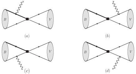
Figure 1: Weak annihilation diagrams for $B^{0}\to\phi\gamma$ decay.

2.1 Contribution from weak annihilation

Now we are ready to investigate the weak annihilation contribution to the purely annihilation type operators. The weak annihilation diagrams are shown in Fig. 1, all of which are mediated by the four-quark operators. In order to produce a transversely polarized vector meson, the four-quark operators must be matched to the $\rm SCET_{I}$ operators which are suppressed by $1/m_{b}$. Among the four diagrams in Fig. 1, diagram (c) is dominant because it is enhanced by a hard-collinear propagator compared with the other diagrams. Therefore we neglect diagrams (a,b,d), which are highly suppressed in our calculation. Only considering the contribution of the leading two particle Fock state of the vector meson, the physical $\rm SCET_{I}$ operator, which can contribute to purely annihilation type decays, is written by

$$Q_{1}=[\bar{\chi}_{\overline{hc}}(s\bar{n})(1+\gamma_{5})\gamma_{\perp}^{\mu}\eta_{\overline{hc}}+h.c.]\bar{\xi}_{hc}W_{hc}(tn)\gamma_{\mu}^{\perp}(1-\gamma_{5})h_{v},$$ (12)

with

$$\eta_{\overline{hc}}=-{1\over in\cdot D_{\overline{hc}}}i\not\!\!D_{{\overline{hc}}\perp}{\not\!n\over 2}\chi_{\overline{hc}}.$$ (13)

Although this operator is suppressed relative to the leading power SCET_I four quark operators, they share the same matching coefficients, since the relevant QCD diagrams in the matching procedure are the same. Therefore, the hard function at one loop level can be extracted from the effective Wilson coefficients in the QCD factorization approach of nonleptonic $B$ decays [28]. Similar to the nonleptonic B decays, the hard function is also convoluted with the vector meson LCDAs defined below

$$\langle V(p,\epsilon_{1})|[\bar{\chi}(s\bar{n})\gamma_{\perp}^{\mu}\eta+h.c.]|0\rangle = f_{V}m_{V}\varepsilon_{1\perp}^{*\mu}\int due^{ius\bar{n}\cdot p}g_{\perp}^{(v)}(u)$$

$$\langle V(p,\epsilon_{1})|[\bar{\chi}(s\bar{n})\gamma_{\perp}^{\mu}\gamma_{5}\eta+h.c.]|0\rangle = {i\over 4}f_{V}m_{V}\epsilon_{\perp}^{\mu\nu}\varepsilon_{1\perp\nu}^{*}\int due^{ius\bar{n}\cdot p}g_{\perp}^{(a)^{\prime}}(u),$$ (14)

with $\epsilon^{\perp}_{\mu\nu}=\epsilon_{\mu\nu\bar{n}n}\,/\,2$. As the hard-collinear part decouples from the soft and collinear part, the factorization for the annihilation diagram also holds. We take $B^{0}\to\phi\gamma$ decay as an example, the matrix element can be factorized as

$$\left\langle\phi(\varepsilon_{1})\gamma(\varepsilon_{2})\left|{\cal H}_{\rm eff}\right|\bar{B}\right\rangle|_{\rm anni.} = -{G_{F}\over\sqrt{2}}V_{tb}V_{td}^{*}\left(\alpha_{3}-{1\over 2}\alpha_{3EW}\right){f_{\phi}m_{\phi}\over E_{\gamma}}$$ (15)

$$\times \langle\gamma(\varepsilon_{2})\left|C_{\rm FF}\bar{\xi}\not\!\varepsilon^{\ast}_{1}(1-\gamma_{5})h_{v}\right|\bar{B}\rangle,$$

where the anti-collinear vector meson LCDA has been convoluted with the hard function, and the effective Wilson coefficients are written by [19]

$$\alpha_{3} = C_{3}+{C_{4}\over N_{c}}+C_{5}+{C_{6}\over N_{c}}+{\alpha_{s}\over 4\pi}{C_{F}\over N_{C}}{f^{\perp}_{V}\over f_{V}}(C_{4}V_{1}+C_{6}V_{2})$$

$$\alpha_{3EW} = C_{7}+{C_{8}\over N_{c}}+C_{9}+{C_{10}\over N_{c}}+{\alpha_{s}\over 4\pi}{C_{F}\over N_{C}}{f^{\perp}_{V}\over f_{V}}(C_{8}V_{2}+C_{10}V_{1})$$ (16)

with the vertex correction term

$$V_{1} = \int_{0}^{1}duT_{1}(u)\left[{1\over 4}g_{\perp}^{(a)^{\prime}}(u)-g_{\perp}^{(v)}(u)\right]$$

$$V_{2} = \int_{0}^{1}duT_{2}(u)\left[{1\over 4}g_{\perp}^{(a)^{\prime}}(u)+g_{\perp}^{(v)}(u)\right],$$

where [30]

$$T_{1}(u) = 12\ln{m_{b}\over\mu}-18+g(u)$$

$$T_{2}(u) = -12\ln{m_{b}\over\mu}+6-g(\bar{u})$$ (17)

$$g(u) = {4-6u\over\bar{u}}\ln u-3i\pi+\left(2{\rm Li_{2}}(u)-\ln^{2}u+{2\ln u\over\bar{u}}-(3+2\pi i)\ln u-[u\to\bar{u}]\right).$$

The hard function $C_{FF}$ arises from matching the weak current $\bar{u}\,\gamma_{\mu\,\perp}\,(1-\gamma_{5})\,b$ onto the corresponding SCET current. The remaining $B\to\gamma$ transition matrix element containing soft and collinear field can be parameterized by

$$\langle\gamma(\varepsilon_{2},p)|C_{\rm FF}\bar{\xi}\gamma_{\mu}(1-\gamma_{5})h_{v}|\bar{B}_{v}\rangle=E_{\gamma}\varepsilon^{*}_{2\nu}(g_{\perp}^{\mu\nu}F_{A}+i\epsilon_{\perp}^{\mu\nu}F_{V}).$$ (18)

The $B\to\gamma$ transition form factors $F_{V,A}$ also present in the $B\to\gamma\ell\nu$ decay, which has been extensively studied [31, 32, 33, 34, 35, 36, 37, 38, 39, 40, 41, 42]. At leading power $F_{A}=F_{V}$ due to the left-handedness of the weak interaction current and helicity-conservation of the quark-gluon interaction in the high-energy limit, and this symmetry relation is broken by power suppressed local contributions. At leading power both hard function and jet function have been calculated up to two-loop level and next-to-leading logarithmic resummation has been performed. The power suppressed symmetry-breaking local contrition and symmetry conserving high-twist contribution and resolve photon contribution are also considered. Utilizing the result of ref.[42] in our calculation, the transition amplitude of $B^{0}\to\phi\gamma$ and $B_{s}\to\rho^{0}(\omega)\gamma$ is then written by

$$A(B\to\phi\gamma)|_{\rm anni} = -{G_{F}\over\sqrt{2}}\lambda_{t}\left(\alpha_{3}-{1\over 2}\alpha_{3EW}\right)ef_{\phi}m_{\phi}(F_{A}g^{\perp}_{\mu\nu}+iF_{V}\epsilon^{\perp}_{\mu\nu})\epsilon_{2}^{*\mu}\epsilon_{1}^{*\mu}$$

$$\sqrt{2}A(B_{s}\to\rho^{0}\gamma)|_{\rm anni} = {G_{F}\over\sqrt{2}}\left(\lambda_{u}\alpha_{2}-{3\over 2}\lambda_{t}\alpha_{3EW}\right)ef_{\rho}m_{\rho}(F_{A}g^{\perp}_{\mu\nu}+iF_{V}\epsilon^{\perp}_{\mu\nu})\epsilon_{2}^{*\mu}\epsilon_{1}^{*\mu}$$ (19)

$$\sqrt{2}A(B_{s}\to\omega\gamma)|_{\rm anni} = {G_{F}\over\sqrt{2}}\left(\lambda_{u}\alpha_{2}-\lambda_{t}\alpha_{3}-{1\over 2}\lambda_{t}\alpha_{3EW}\right)ef_{\omega}m_{\omega}(F_{A}g^{\perp}_{\mu\nu}+iF_{V}\epsilon^{\perp}_{\mu\nu})\epsilon_{2}^{*\mu}\epsilon_{1}^{*\mu},$$

where

$$\alpha_{2} = C_{2}+{C_{1}\over N_{c}}+{\alpha_{s}\over 4\pi}{C_{F}\over N_{C}}{f^{\perp}_{V}\over f_{V}}C_{2}V_{1}.$$ (20)

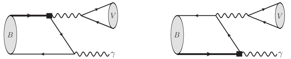
Figure 2: Production of a vector meson via electromagnetic penguin operator

2.2 Contribution from electro-magnetic penguin operator

The annihilation diagram is power suppressed because leading power four-quark operators cannot contribute to transversely polarized vector meson. However, if the power suppressed operator $\bar{\chi}\gamma_{\perp}\eta\sim\lambda^{3/2}$ is replaced by a photon field $\not\!\!\!{\cal A}^{em}_{\perp}\sim\lambda^{1/2}$, this will leads to a large enhancement factor $m_{b}/\Lambda$. Furthermore, for the pure annihilation type decays such as the $B^{0}\to\phi\gamma$, the rather small color suppressed penguin operator Wilson coefficient will also be replaced by $C_{7\gamma}$, at the cost of an electro-magnetic coupling constant $\alpha_{em}$. The leading order Feynman diagrams of the electro-magnetic penguin operator contribution are plotted in Fig. 2. They are corresponding to the matrix element

$$A^{\rm LO}_{\rm EMP} = \,-{G_{F}\over\sqrt{2}}\lambda_{t}\,\int d^{4}x\,\,\langle\phi(p,\epsilon_{1}^{\ast})\gamma(q,\epsilon_{2}^{\ast})|{\rm T}\left\{Q_{q}e\bar{q}\not{A}q(x),C_{7\gamma}O_{7\gamma}(0)\right\}|\bar{B}(v)\rangle$$ (21)

$$+\left[p\leftrightarrow q\right]\,.$$

To evaluate this amplitude, one must have the knowledge of the matrix element of $O_{7\gamma}$. When the photon field is sandwiched between the vector meson state and the vacuum, the matrix element reads [43]

$$\langle V|e{\cal A}^{\rm em}_{\perp\mu}|0\rangle=-{2\over 3}ia_{V}{e^{2}f_{V}\over m_{V}}\varepsilon_{\perp\mu}^{*}$$ (22)

with $a_{\rho}=3/2,a_{\omega}=1/2,a_{\phi}=-1/2$. Taking advantage of the above matrix element, the leading order result can be obtained, which has been given in [20].

In this work, we make improvement by taking the QCD correction of the Wilson coefficients of $O_{7\gamma}$ operator into account. The complete ${\cal O}(\alpha_{s})$ corrections including the contribution from four-quark operators and chromo-magnetic operator are accomplished in [44]. Similar to the decay amplitude of $B^{0}\to\gamma\gamma$ [45] and $B^{0}\to\gamma\ell\ell$ mode [46], the leading power contribution of electro-magnetic dipole operator to $B^{0}\to\phi\gamma$ and $B_{s}\to\rho^{0}(\omega)\gamma$ decay can be expressed as

$${A}_{\rm EMP} = i\,{4\,G_{F}\over\sqrt{2}}\lambda_{t}\,{\alpha_{\rm em}\over 4\pi}\left({-{2\over 3}ia_{V}}\right){ef_{V}\over m_{V}}\,\varepsilon_{1}^{\ast\alpha}(p)\,\varepsilon_{2}^{\ast\beta}(q)\,\left[g_{\alpha\beta}^{\perp}+i\epsilon_{\alpha\beta}^{\perp}\right]\,Q_{q}\,f_{B_{q}}\,m_{B_{q}}E_{\gamma}\bar{m}_{b}V_{7}^{eff}(0)$$ (23)

$$\times \left[{V_{7}^{eff}(q^{2})\over V_{7}^{eff}(0)}\dfrac{m_{B_{q}}}{2E_{\gamma}}\int_{0}^{\infty}{d\omega\over\omega}J(2E_{\gamma},0,\omega)\phi^{B}_{+}(\omega)\right.$$

$$+\left.\int_{0}^{\infty}{d\omega\over\omega-{m_{V}^{2}/m_{B_{q}}}}J(2E_{\gamma},m_{V}^{2},\omega)\phi^{B}_{+}(\omega)\right].$$

The explicit expression of effective Wilson coefficient $V_{7}^{eff}(q^{2})$ and the jet function $J(2E_{\gamma},q^{2},\omega)$ at one loop level are given in [46], including the factorization scale dependence obtained from renormalization group evolution. In our numerical analysis, the factorization scale is chosen at an intermediate scale $\mu_{hc}\sim\sqrt{E_{\gamma}\omega}$ .

2.3 Contribution from mixing of neutral vector mesons

The mixing of the flavor-SU(3) singlet and octet states of vector mesons to form mass eigenstates is of fundamental importance in hadronic physics. It is commonly accepted that the vector meson states satisfy the “ideal” mixing, close to the value that would lead to the complete decoupling of the light $u$ and $d$ quarks from the heavier $s$ quark in the resultant mass eigenstates $\omega$ and $\phi$. Actually $\omega$ and $\phi$ are not pure states with definite isospin given by

$$|\omega_{I}\rangle=\frac{1}{\sqrt{2}}(|\bar{u}u\rangle+|\bar{d}d\rangle)\,,\qquad|\phi_{I}\rangle=|\bar{s}s\rangle\,.$$ (24)

The mass eigenstates $\omega,\phi$ deviate from the “ideal” states $\omega_{I},\phi_{I}$ through a mixing matrix

$$\left(\begin{array}[]{c}|\omega\rangle\\ |\phi\rangle\end{array}\right)=\left(\begin{array}[]{cc}\cos\delta&\sin\delta\\ -\sin\delta&\cos\delta\end{array}\right)\left(\begin{array}[]{c}|\omega_{I}\rangle\\ |\phi_{I}\rangle\end{array}\right),$$ (31)

where the mixing angle $\delta$ can be determined from the experimental data or by model calculation. The isospin triplet $\rho^{0}$ can also mix with $\omega$ and $\phi$ through electro-magnetic interactions, however, the mixing angle is about one order smaller than the $\omega-\phi$ mixing, since the isospin-breaking is much smaller than the flavor SU(3) breaking effect. Thus we do not take this isospin-breaking mixing effect into account in our analysis. After considering the mixing between $\omega$ and $\phi$ meson, the $B^{0}\to\phi\gamma$ and $B_{s}\to\omega\gamma$ decays can be expressed in terms of the decay amplitude with the ideal mixing meson final state, i.e.,

$$A(B^{0}\to\phi\gamma)|_{mixing} = -\sin\delta A(B\to\omega_{I}\gamma)$$

$$A(B_{s}\to\omega\gamma)|_{mixing} = \sin\delta A(B_{s}\to\phi_{I}\gamma).$$ (32)

Table 1: Estimation of the relative size from different contributions to $B^{0}\to\phi\gamma$.

Contributions	Suppression	Enhancement	Typical value
${|A(B\to\phi\gamma)|_{\rm anni}\over|A(B\to\rho^{0}\gamma)|_{\rm LP}}$	${{\alpha_{3}-1/2\alpha_{3EW}}\over C_{7\gamma}}\times{m_{V}\over m_{b}}$	-	0.004
${|A(B\to\phi\gamma)|_{\rm EMP}\over|A(B\to\rho^{0}\gamma)|_{\rm LP}}$	$\alpha_{\rm em}\times a_{\phi}$	${m_{b}\over m_{V}}$	$0.01$
${|A(B\to\phi\gamma)|_{\rm mixing}\over|A(B\to\rho^{0}\gamma)|_{\rm LP}}$	$\sin\delta$	-	0.06

To show that the $\omega-\phi$ meson mixing will dominate the $B^{0}\to\phi\gamma$ and $B_{s}\to\omega\gamma$ decays, we estimate the relative size of different contributions to these decay modes. For convenience, we investigate the proportion of the absolute value of the amplitude of each contribution with respect to the absolute value of the leading power amplitude in $B\to\rho^{0}\gamma$ decay in Table 1. From this table we can see that the mixing effect can increase the branching ratio from annihilation topology in QCD factorization approach over two orders of magnitudes, and is one order larger than the contribution from electro-magnetic operators. For $B_{s}\to\rho^{0}(\omega)\gamma$ decays, the tree operators with large Wilson coefficient can contribute, while they are suppressed by a small suppression factor from CKM matrix elements, i.e., $|V_{ub}V_{us}/V_{tb}V_{ts}|$, therefore, the relative size of different type of contribution in $B_{s}\to\rho^{0}(\omega)\gamma$ decays is similar to $B\to\phi\gamma$.

3 Numerical analysis

3.1 Input parameters

The decay amplitudes for the $B^{0}\to\phi\gamma$ and $B_{s}\to\rho^{0}(\omega)\gamma$ decays have been obtained in the previous section, they will be utilized to predict the branching ratios of these decay modes. Firstly we specify the input parameters which will be used in the numerical calculation. Among various parameters, the mixing angle $\delta$ is of unique importance because it will provide the major source of uncertainties in our calculations. The mixing angle has been discussed in many phenomenological methods such as the framework of the hidden local symmetry Lagrangian [47, 48], the chiral perturbation theory [49, 50], the light front quark model [51] and the Nambu-Jona-Lasinio model [52, 53] etc., with the obtained values varying at the interval about $3^{\circ}\sim 5^{\circ}$ (most of the studies prefer $[3^{\circ},4^{\circ}]$). In this work, we adopt the value of mixing angle as $\delta=3.5^{\circ}\pm 0.5^{\circ}$.

To arrive at the result of the decay amplitudes from the $\omega-\phi$ mixing, the leading power contribution of $B^{0}\to\omega\gamma$ and $B_{s}\to\phi\gamma$ is necessary. The basic nonperturbative inputs in these amplitudes are the soft form factor $\zeta^{\rm BV}_{\perp}$ and the light-cone distribution amplitude of $B$-meson and $\rho,\omega,\phi$ meson. The soft factors $\zeta^{\rm BV}_{\perp}$ defined in terms of the matrix element of SCET_I operators have been calculated using SCET sum rules. The complete NLO corrections to the correlation function as well as the power suppressed higher twist contribution have been calculated in ref.[54]. The result is adopted as $\zeta^{\rm BV}_{\perp}=0.33\pm 0.10$. For the $B_{s}\to\phi$ transition, the result is $\zeta^{\rm B_{s}V}_{\perp}=0.35\pm 0.10$, allowing a small SU(3) breaking effect.

For the leading twist two-particle $B$-meson distribution amplitude, we will employ the following three-parameter model

$$\phi_{B}^{+}(\omega)={\Gamma(\beta)\over\Gamma(\alpha)}\,{\omega\over\omega^{2}_{0}}\,e^{-{\omega\over\omega_{0}}}\,U\left(\beta-\alpha,3-\alpha,{\omega\over\omega_{0}}\right),$$ (33)

where $U(\alpha,\gamma,x)$ is the confluent hypergeometric function of the second kind. A special case is the exponential model when $\alpha=\beta$

$$\phi^{+}_{B}(\omega)={\omega\over\omega^{2}_{0}}\,e^{-{\omega\over\omega_{0}}}.$$ (34)

To estimate the error from the models, we will let $\alpha-\beta$ vary at the region $-0.5<\alpha-\beta<0.5$, then we employ two models with $\alpha=2.0,\beta=1.5$ and $\alpha=1.5,\beta=2.0$. The parameter $\omega_{0}$ is closely related to the first inverse moment $1/\lambda_{B}$, whose determination has been discussed extensively in the context of exclusive $B$-meson decays (see [55, 56, 57, 54] for more discussions). Here we will employ $\lambda_{B}(1\,{\rm GeV})=0.35\pm 0.05\,{\rm GeV}$ and $\lambda_{B_{s}}(1\,{\rm GeV})=0.40\pm 0.05\,{\rm GeV}$. For the light vector meson, the leading twist LCDAs can be expanded in terms of Gegenbauer polynomials due to the behavior of scale evolution, i.e.

$$\phi_{V}(x) = 6x(1-x)[1+a_{V}C_{2}^{3/2}(2x-1)]$$

$$\phi_{V_{\perp}}(x) = 6x(1-x)[1+a_{V_{\perp}}C_{2}^{3/2}(2x-1)].$$ (35)

For the power suppressed vector meson LCDAs, ignoring the three parton wave function, we have the following expression [58]

$${1\over 4}g_{\perp}^{(a)^{\prime}}(u)-g_{\perp}^{(v)}(u)=-\int_{0}^{u}{\phi_{V}(v)\over\bar{v}},\,\,\,\,\,{1\over 4}g_{\perp}^{(a)^{\prime}}(u)+g_{\perp}^{(v)}(u)=\int_{u}^{1}{\phi_{V}(v)\over v}.$$ (36)

In the annihilation topology, the $B_{(s)}\to\gamma$ transition form factors $F_{V,A}$ is required. The SU(3) breaking effect is found to be negligible after taking the next-to-leading power contribution into account, thus we adopt the same result for both $B$ and $B_{s}$ decays, i.e., $F_{V}=0.23\pm 0.07$, $F_{A}=0.21\pm 0.07$. The values of the other parameters are presented in Table 2.

Table 2: Input parameters

$\tau_{B^{0}}$	1.52ps	$G_{F}$	$1.116637\times 10^{-5}$
$\tau_{B_{s}}$	1.51ps	$\lambda$	0.22650
$f_{B}$	0.192	$\bar{\rho}$	0.141
$f_{B_{s}}$	0.230	$A$	0.790
$\sigma^{(1)}_{B}$	$1.63\pm 0.15$	$\bar{\eta}$	0.357
$\sigma^{(1)}_{B_{s}}$	$1.49\pm 0.15$
$f_{\rho}$(1GeV)	0.216$\pm$ 0.003	$a_{2\rho}$(1GeV)	0.15$\pm$0.07
$f_{\omega}$(1GeV)	0.187$\pm$0.005	$a_{2\omega}$(1GeV)	0.15$\pm$0.07
$f_{\phi}$(1GeV)	0.215$\pm$0.005	$a_{2\phi}$(1GeV)	0.18$\pm$0.08
$f_{\rho\perp}$(1GeV)	0.165$\pm$ 0.009	$a_{2\rho\perp}$(1GeV)	0.14$\pm$0.06
$f_{\omega\perp}$(1GeV)	0.151$\pm$0.009	$a_{2\omega\perp}$(1GeV)	0.14$\pm$0.06
$f_{\phi\perp}$(1GeV)	0.186$\pm$0.009	$a_{2\phi\perp}$(1GeV)	0.14$\pm$0.07

3.2 Phenomenological predictions

Collecting all the contributions to the factorization amplitudes calculation in the previous section together, we arrive at the final expression of the decay amplitudes for the pure annihilation type $B\to V\gamma$ decays

$$\begin{aligned} &A(B^{0}\to\phi\gamma)=\cos\delta[A(B^{0}\to\phi_{I}\gamma)|_{\rm anni}+A(B^{0}\to\phi_{I}\gamma)|_{\rm EMP}]-\sin\delta A(B\to\omega_{I}\gamma)\\ &A(B_{s}\to\omega\gamma)=\cos\delta[A(B_{s}\to\omega_{I}\gamma)|_{\rm anni}+A(B_{s}\to\omega_{I}\gamma)|_{\rm EMP}]+\sin\delta A(B_{s}\to\phi_{I}\gamma)\\ &A(B_{s}\to\rho^{0}\gamma)=A(B_{s}\to\rho^{0}\gamma)|_{\rm anni}+A(B_{s}\to\rho^{0}\gamma)|_{\rm EMP}.\end{aligned}$$ (37)

The results for the phenomenological observables in pure annihilation type decays are then studied. As the decay rates are relatively small and the observables such as CP asymmetry are hard to be detected, we concentrate on the CP-averaged branching ratios defined below

$$\langle B(B^{0}\to V\gamma)\rangle={B(\bar{B}^{0}\to V\gamma)+B(B^{0}\to V\gamma)\over 2},$$ (38)

where the specific expression of the branching ratio is give by

$$B(\bar{B}^{0}\to V\gamma)=\dfrac{\tau_{B}}{16\pi m_{B}}\bigg{(}1-\dfrac{m_{V}^{2}}{m_{B}^{2}}\bigg{)}|A(\bar{B}^{0}\rightarrow V\gamma)|^{2}.$$ (39)

To illustrate the contribution from various sources, we firstly present the results of each kind of contributions in Table 3. In the contribution from mixing of neutral vector mesons, we only consider the leading power contribution to the $B^{0}\to\omega_{I}\gamma$ and $B_{s}\to\phi_{I}\gamma$ amplitudes, because the mixing angle is already a small quantity. The QCD factorization result of the pure annihilation contribution is consistent with the result in [19]. The contribution from elector-magnetic penguin operator is a bit larger than our previous predictions in [20] as the leading logarithm resummation of effective Wilson coefficient $C_{7eff}$ is employed and some parameters are renewed. Our results indicate that the branching ratio of $B^{0}\to\phi\gamma$ purely from the $\phi-\omega$ mixing is three orders larger than that from the annihilation topology, and also about two orders larger than that from the electro-magnetic penguin contribution in the decays. Apparently this result is consistent with our rough estimation. Taking advantage of the central values in Table 1, the total branching ratio of $B^{0}\to\phi\gamma$ is obtained as $3.99\times 10^{-9}$, which have the chance to be measured in the Belle-II with an ultimate integrated luminosity of $50ab^{-1}$. The $B_{s}\to\omega\gamma$ decay with the branching ratio $2.01\times 10^{-7}$ can also confront the LHC-b data.

Table 3: Branching fractions of different contributions.

Channels	$A_{anni}$ Only	$A_{EMP}$ Only	$A_{mixing}$ Only	Total
$B(B^{0}\rightarrow\phi\gamma)$	$3.93\times 10^{-12}$	$2.02\times 10^{-11}$	$3.61\times 10^{-9}$	$3.99\times 10^{-9}$
$B(B_{s}^{0}\rightarrow\omega^{0}\gamma)$	$6.94\times 10^{-11}$	$3.91\times 10^{-10}$	$1.80\times 10^{-7}$	$2.01\times 10^{-7}$
$B(B_{s}^{0}\rightarrow\rho^{0}\gamma)$	$4.89\times 10^{-11}$	$4.79\times 10^{-9}$	-	$5.67\times 10^{-9}$

We define the following ratios of branching fractions, which can highlight the importance of the vector meson mixing effects

$$R_{\rho\omega}={B(B_{s}^{0}\rightarrow\rho^{0}\gamma)\over B(B_{s}^{0}\rightarrow\omega^{0}\gamma)},\,\,\,R_{\rho\phi}={B(B_{s}^{0}\rightarrow\rho^{0}\gamma)\over B(B^{0}\rightarrow\phi\gamma)}.$$ (40)

Naively considering, the first ratio $R_{\rho\omega}\sim 1$, since the Feynman diagrams of the annihilation topology are the same for $B_{s}\to\rho^{0}\gamma$ and $\omega\gamma$ decays, furthermore, the contribution from electro-magnetic penguin will even enhance this ratio to 10, as $|a_{\rho}/a_{\omega}|=3$. The second ratio $R_{\rho\phi}$ is expected to be large for the CKM enhancement from the ratio $|V_{tb}V_{ts}/V_{tb}V_{td}|^{2}$. While after the $\phi-\omega$ mixing effect is taken into account, the values of these ratios are dramatically changed. Our result shows that $R_{\rho\omega}\simeq 0.03$ which confirms the dominance of meson mixing effects, and $R_{\rho\phi}\simeq 1.4$ which indicates that the contribution from $\omega-\phi$ mixing is larger than the electro-magnetic penguin amplitude by a factor $|V_{tb}V_{ts}/V_{tb}V_{td}|$ approximately. The predicted values of these ratios are expected to be tested in the future experiments.

Now we investigate the theoretical uncertainties. Inspecting the distinct sources of the yielding theory uncertainties as collected in the following formula, we have

$$B(B^{0}\rightarrow\phi\gamma) = 3.99\;^{+1.19}_{-1.04}|_{\zeta_{\perp}}\;^{+1.16}{}_{-1.01}|_{\delta}\;^{+0.02}{}_{-0.02}|_{f_{V},\phi_{V}}\;^{+0.08}{}_{-0.06}|_{\lambda_{B}}\;^{+0.07}{}_{-0.15}|_{\phi_{B}}\;^{+0.01}{}_{-0.01}|_{F_{V}}\;^{+0.01}{}_{-0.01}|_{F_{A}}\times 10^{-9},$$

$$B(B_{s}\rightarrow\omega\gamma) = 2.01\;^{+0.56}_{-0.49}|_{\zeta_{\perp}}\;^{+0.58}{}_{-0.51}|_{\delta}\;^{+0.01}{}_{-0.01}|_{f_{V},\phi_{V}}\;^{+0.02}{}_{-0.02}|_{\lambda_{B}}\;^{+0.00}{}_{-0.02}|_{\phi_{B}}\;^{+0.01}{}_{-0.01}|_{F_{V}}\;^{+0.01}{}_{-0.01}|_{F_{A}}\times 10^{-7},$$

$$B(B_{s}\rightarrow\rho^{0}\gamma) = 5.67\;^{+0.16}_{-0.16}|_{f_{V},\phi_{V}}\;^{+0.55}{}_{-0.41}|_{\lambda_{B}}\;^{+1.50}{}_{-1.69}|_{\phi_{B}}\;^{+0.04}{}_{-0.04}|_{\sigma_{B}}\;^{+0.15}{}_{-0.15}|_{F_{V}}\;^{+0.15}{}_{-0.15}|_{F_{A}}\times 10^{-9}.$$ (41)

It is obvious that the soft form factors which play the dominant role in the $B\to\omega\gamma$ and $B_{s}\to\phi\gamma$ decays provides an important source of uncertainties. The mixing angle between $\phi$ and $\omega$ meson is another major source of uncertainty as expected. As the decay amplitudes of $B\to\phi\gamma$ and $B_{s}\to\omega\gamma$ are very sensitive to the vector meson mixing effect, these channels can serve as a good platform to determine the mixing angle, i.e., the mixing angle between $\omega$ and $\phi$ meson can be determined by

$$\sin\delta\simeq\sqrt{B(B^{0}\rightarrow\phi\gamma)\over B(B^{0}\rightarrow\omega\gamma)}\,\,\,or\,\,\,\sqrt{B(B_{s}^{0}\rightarrow\omega\gamma)\over B(B_{s}^{0}\rightarrow\phi\gamma)},$$ (42)

if the related decay modes are measured. For the $B(B_{s}\rightarrow\rho^{0}\gamma)$ decay which is dominated by the electro-magnetic penguin operator, the major source of uncertainty is from the shape and the first inverse moment of the LCDA of $B_{s}$ meson. Therefore, it is of great importance to improve the study of $B_{(s)}$ meson LCDA. A recent effort is the introduction of the quasi-parton distribution amplitude of $B$ meson [59] so that it can be calculated by lattice QCD simulation.

4 Closing remarks

The pure annihilation type radiative B meson decays, including $B^{0}\to\phi\gamma$ and $B_{s}\to\rho^{0}(\omega)\gamma$ decays, are very rare in the standard model, which makes them very sensitive to the new physics signals beyond the standard model. We reviewed factorization of $B\to V\gamma$ decays at leading power using SCET, and derived the factorization formula for annihilation topology. The electro-magnetic penguin contribution to the pure annihilation radiative decays, which is power enhanced, is also revisited with leading logarithm resummation of the effective Wilson coefficients taken into account. As the major subject of this work, we studied the contribution of the neutral vector meson $\omega-\phi$ mixing to the decay amplitudes. Although the mixing angle of the $\phi-\omega$ is only a few percent, this contribution owns larger Wilson coefficients as well as power enhancement compared with annihilation topology. A rough estimate indicates that the contribution from $\phi-\omega$ mixing is dominant in the pure annihilation radiative decays. The numerical calculation shows that the branching ratio of $B^{0}\to\phi\gamma$ purely from the $\phi-\omega$ mixing is three orders larger than that from the annihilation topology, and also two orders larger than that from the electro-magnetic penguin contribution in the decays. The similar hierarchy between the different contributions holds for $B^{0}\to\omega\gamma$. The decay rate of $B_{s}\to\rho^{0}\gamma$ is much smaller than that of $B_{s}\to\omega\gamma$ for the suppressed mixing effect is not considered. The new defined ratios $R_{\rho\omega}\simeq 0.03$ and $R_{\rho\phi}\simeq 1.4$ further highlight the importance of the mixing effect. The predicted branching ratios of $B^{0}\to\phi\gamma$ and $B_{s}\to\rho^{0}(\omega)\gamma$ decays are given below:

$$B(B^{0}\rightarrow\phi\gamma) = 3.99^{+1.67}_{-1.46}\times 10^{-9},$$

$$B(B_{s}\rightarrow\omega\gamma) = 2.01^{+0.81}_{-0.71}\times 10^{-7},$$ (43)

$$B(B_{s}\rightarrow\rho^{0}\gamma) = 5.67^{+1.62}_{-1.76}\times 10^{-9}.$$

These results are to be tested by the Belle-II and LHC-b experiments.

References

• [1] T. Hurth Rev. Mod. Phys.  75 (2003) 1159 [arXiv:hep-ph/0212304].
• [2] M. Misiak, H. M. Asatrian, K. Bieri, M. Czakon, A. Czarnecki, T. Ewerth, A. Ferroglia, P. Gambino, M. Gorbahn and C. Greub, et al. Phys. Rev. Lett. 98, 022002 (2007) [arXiv:hep-ph/0609232 [hep-ph]].
• [3] M. Misiak and M. Steinhauser, Nucl. Phys. B 683 (2004) 277 [arXiv:hep-ph/0401041];
M. Gorbahn and U. Haisch, Nucl. Phys. B 713 (2005) 291 [arXiv:hep-ph/0411071];
M. Gorbahn, U. Haisch and M. Misiak, Phys. Rev. Lett.  95 (2005) 102004 [arXiv:hep-ph/0504194];
M. Misiak and M. Steinhauser, Nucl. Phys. B 764, 62-82 (2007) [arXiv:hep-ph/0609241 [hep-ph]].
• [4] M. Beneke, T. Feldmann and D. Seidel, Nucl. Phys. B 612, 25-58 (2001) [arXiv:hep-ph/0106067 [hep-ph]].
• [5] M. Beneke, T. Feldmann and D. Seidel, Eur. Phys. J. C 41, 173-188 (2005) [arXiv:hep-ph/0412400 [hep-ph]].
• [6] A. Ali and A. Y. Parkhomenko, Eur. Phys. J. C 23 (2002) 89 [arXiv:hep-ph/0105302];
A. Ali, E. Lunghi and A. Y. Parkhomenko, Phys. Lett. B 595 (2004) 323 [arXiv:hep-ph/0405075];
• [7] A. Ali and A. Parkhomenko, [arXiv:hep-ph/0610149 [hep-ph]].
• [8] S. W. Bosch and G. Buchalla, Nucl. Phys. B 621 (2002) 459 [arXiv:hep-ph/0106081].
• [9] S. W. Bosch, arXiv:hep-ph/0208203.
• [10] S. W. Bosch and G. Buchalla, JHEP 0501 (2005) 035 [arXiv:hep-ph/0408231].
• [11] P. Ball and R. Zwicky, JHEP 0604 (2006) 046 [arXiv:hep-ph/0603232].
• [12] T. Becher, R. J. Hill and M. Neubert, Phys. Rev. D 72 (2005) 094017 [arXiv:hep-ph/0503263].
• [13] Y.Y. Keum, M. Matsumori and A.I. Sanda, Phys. Rev. D 72 (2005) 014013 [arXiv:hep-ph/0406055];
C.D. Lu, M. Matsumori, A.I. Sanda and M.Z. Yang, Phys. Rev. D 72 (2005) 094005 [Erratum-ibid. D 73 (2006) 039902] [arXiv:hep-ph/0508300];
M. Matsumori and A.I. Sanda, Phys. Rev. D 73 (2006) 114022 [arXiv:hep-ph/0512175];
W. Wang, R.H. Li and C.D. Lu, [arXiv:0711.0432 [hep-ph]].
• [14] D. Atwood, M. Gronau and A. Soni, Phys. Rev. Lett.  79 (1997) 185 [arXiv:hep-ph/9704272].
• [15] B. Grinstein, Y. Grossman, Z. Ligeti and D. Pirjol, Phys. Rev. D 71 (2005) 011504 [arXiv:hep-ph/0412019].
• [16] B. Grinstein and D. Pirjol, Phys. Rev. D 73 (2006) 014013 [arXiv:hep-ph/0510104].
• [17] P. Ball and R. Zwicky, Phys. Lett. B 642 (2006) 478 [arXiv:hep-ph/0609037].
• [18] A. L. Kagan and M. Neubert, Phys. Lett. B 539 (2002) 227 [arXiv:hep-ph/0110078].
• [19] X. q. Li, G. r. Lu, R. m. Wang and Y. D. Yang, Eur. Phys. J. C 36, 97 (2004) [hep-ph/0305283].
• [20] C. D. Lü, Y. L. Shen and W. Wang, Chin. Phys. Lett.  23, 2684 (2006) [hep-ph/0606092].
• [21] Y. Li and C. D. Lü, Phys. Rev. D 74 (2006) 097502 [arXiv:hep-ph/0605220];
• [22] P. A. Zyla et al. [Particle Data Group], Review of Particle Physics, PTEP 2020 (2020) 083C01.
• [23] M. Gronau and J. L. Rosner, Phys. Lett. B 666 (2008), 185-188 [arXiv:0806.3584 [hep-ph]].
• [24] M. Gronau and J. L. Rosner, Phys. Rev. D 79 (2009), 074006 [arXiv:0902.1363 [hep-ph]].
• [25] Y. Li, C. D. Lü and W. Wang, Phys. Rev. D 80, 014024 (2009) [arXiv:0901.0648 [hep-ph]].
• [26] G. Buchalla, A. J. Buras and M. E. Lautenbacher, Rev. Mod. Phys.  68 (1996) 1125 [arXiv:hep-ph/9512380].
• [27] C. Greub, T. Hurth and D. Wyler, Phys. Rev. D 54 (1996) 3350 [arXiv:hep-ph/9603404];
A. J. Buras, A. Czarnecki, M. Misiak and J. Urban, Nucl. Phys. B 611 (2001) 488 [arXiv:hep-ph/0105160] and Nucl. Phys. B 631 (2002) 219 [arXiv:hep-ph/0203135].
• [28] M. Beneke, G. Buchalla, M. Neubert and C. T. Sachrajda, Nucl. Phys. B 591 (2000), 313-418 [arXiv:hep-ph/0006124 [hep-ph]].
• [29] M. Beneke, A. P. Chapovsky, M. Diehl and T. Feldmann, Nucl. Phys. B 643 (2002) 431 [hep-ph/0206152].
• [30] M. Beneke, J. Rohrer and D. Yang, Nucl. Phys. B 774, 64-101 (2007) [arXiv:hep-ph/0612290 [hep-ph]].
• [31] E. Lunghi, D. Pirjol and D. Wyler, Nucl. Phys. B 649 (2003) 349 [hep-ph/0210091].
• [32] S. W. Bosch, R. J. Hill, B. O. Lange and M. Neubert, Phys. Rev. D 67 (2003) 094014 [hep-ph/0301123].
• [33] M. Beneke and J. Rohrwild, Eur. Phys. J. C 71 (2011) 1818 [arXiv:1110.3228 [hep-ph]].
• [34] V. M. Braun and A. Khodjamirian, Phys. Lett. B 718 (2013) 1014 [arXiv:1210.4453 [hep-ph]].
• [35] Y. M. Wang, JHEP 1609 (2016) 159 [arXiv:1606.03080 [hep-ph]].
• [36] P. Ball and E. Kou, JHEP 04 (2003), 029 [arXiv:hep-ph/0301135 [hep-ph]].
• [37] Y. M. Wang and Y. L. Shen, JHEP 05 (2018), 184 [arXiv:1803.06667 [hep-ph]].
• [38] M. Beneke, V. M. Braun, Y. Ji and Y. B. Wei, JHEP 07 (2018), 154 [arXiv:1804.04962 [hep-ph]].
• [39] Y. L. Shen, Z. T. Zou and Y. B. Wei, Phys. Rev. D 99 (2019) no.1, 016004 [arXiv:1811.08250 [hep-ph]].
• [40] Z. L. Liu and M. Neubert, JHEP 06 (2020), 060 [arXiv:2003.03393 [hep-ph]].
• [41] A. M. Galda and M. Neubert, Phys. Rev. D 102 (2020), 071501 [arXiv:2006.05428 [hep-ph]].
• [42] Y. L. Shen, Y. B. Wei, X. C. Zhao and S. H. Zhou, Chin. Phys. C 44, no.12, 123106 (2020) [arXiv:2009.03480 [hep-ph]].
• [43] M. Beneke, J. Rohrer and D. Yang, Phys. Rev. Lett.  96, 141801 (2006) [hep-ph/0512258].
• [44] K. G. Chetyrkin, M. Misiak and M. Munz, Phys. Lett. B 400 (1997) 206; Erratum: [Phys. Lett. B 425 (1998) 414] [hep-ph/9612313].
• [45] Y. L. Shen, Y. M. Wang and Y. B. Wei, JHEP 12, 169 (2020) [arXiv:2009.02723 [hep-ph]].
• [46] M. Beneke, C. Bobeth and Y. M. Wang, JHEP 12, 148 (2020) [arXiv:2008.12494 [hep-ph]].
• [47] M. Benayoun, P. David, L. DelBuono, O. Leitner and H. B. O’Connell, Eur. Phys. J. C 55, 199-236 (2008) [arXiv:0711.4482 [hep-ph]].
• [48] M. Benayoun, P. David, L. DelBuono and O. Leitner, Eur. Phys. J. C 65, 211-245 (2010) [arXiv:0907.4047 [hep-ph]].
• [49] F. Klingl, N. Kaiser and W. Weise, Z. Phys. A 356, 193-206 (1996) [arXiv:hep-ph/9607431 [hep-ph]].
• [50] A. Kucukarslan and U. G. Meissner, Mod. Phys. Lett. A 21, 1423-1430 (2006) [arXiv:hep-ph/0603061 [hep-ph]].
• [51] H. M. Choi, C. R. Ji, Z. Li and H. Y. Ryu, Phys. Rev. C 92, no.5, 055203 (2015) [arXiv:1502.03078 [hep-ph]].
• [52] U. Vogl and W. Weise, Prog. Part. Nucl. Phys. 27, 195-272 (1991)
• [53] S.P. Klevansky, Rev. Mod. Phys. 64, 649-708 (1992)
• [54] J. Gao, C.D. Lü, Y.L. Shen, Y.M. Wang and Y.B. Wei, Phys. Rev. D 101, no.7, 074035 (2020) [arXiv:1907.11092 [hep-ph]].
• [55] Y.M. Wang and Y.L. Shen, Nucl. Phys. B 898 (2015) 563 [arXiv:1506.00667 [hep-ph]].
• [56] Y.M. Wang, Y.B. Wei, Y.L. Shen and C.D. Lü, JHEP 1706 (2017) 062 [arXiv:1701.06810 [hep-ph]].
• [57] C.D. Lü, Y.L. Shen, Y.M. Wang and Y. B. Wei, JHEP 01, 024 (2019) [arXiv:1810.00819 [hep-ph]].
• [58] H.Y. Cheng and K.C. Yang, Phys. Rev. D 78, 094001 (2008) [erratum: Phys. Rev. D 79, 039903 (2009)] [arXiv:0805.0329 [hep-ph]].
• [59] W. Wang, Y. M. Wang, J. Xu and S. Zhao, Phys. Rev. D 102, no.1, 011502 (2020) [arXiv:1908.09933 [hep-ph]].