On the asymptotic decay of the Schrödinger–Newton ground state

Abstract

The asymptotics of the ground state $u(r)$ of the Schrödinger–Newton equation in $\mathbb{R}^{3}$ was determined by V. Moroz and J. van Schaftingen to be $u(r)\sim Ae^{-r}/r^{1-\|u\|_{2}^{2}/8\pi}$ for some $A>0$, in units in which the ground state energy is $-1$. They left open the value of $\|u\|_{2}^{2}$, the squared $L^{2}$ norm of $u$. Here it is rigorously shown that $2^{1/3}3\pi^{2}\leqslant\|u\|_{2}^{2}\leqslant{\color[rgb]{1,0,0}8}\pi^{3/2}$. It is reported that numerically $\|u\|_{2}^{2}\approx 14.03\pi$, revealing that the monomial prefactor of $e^{-r}$ increases with $r$ in a concave manner. Asymptotic results are proposed for the Schrödinger–Newton equation with external $\sim-K/r$ potential, and for the related Hartree equation of a bosonic atom or ion.

    1

     

I Introduction

The non-linear integro-differential equation

$$-\Delta u({\boldsymbol{{s}}})+u({\boldsymbol{{s}}})=\displaystyle{\frac{1}{4\pi}\int_{\mathbb{R}^{3}}\frac{1}{\big{|}{\boldsymbol{{s}}}-{\boldsymbol{{s}}}^{\prime}\big{|}}|u|^{2}({\boldsymbol{{s}}}^{\prime})d^{3}\!s^{\prime}}\,u({\boldsymbol{{s}}})\vspace{-5pt}$$ (1)

shows up in a variety of models in physics, and as such is variously known as Pekar’s equation, Choquard’s equation, Schrödinger–Newton equation, and by other names as well. Pekar Pek suggested it as an approximate model for H. Fröhlich’s condensed matter polaron FrA , FrB ; subsequently it was derived in a suitable limit $N\to\infty$ from $N$-body QM, see DVa , DVb , LT . Choquard proposed it to characterize a self-trapped electron in a one-component quantum plasma; cf. LiebC , ChStV . The name Schrödinger–Newton equation was coined by R. Penrose in his proposal that quantum-mechanical wave function collapse is caused by gravity Pen . It also occurs in the theory of hypothetical bosonic stars in the context of the dark matter mystery; it can be derived from QM of $N$ gravitating spin-zero bosons by taking a Hartree limit $N\to\infty$, see Lewin and references therein. A survey of rigorous results for equation (1) and some of its generalizations is in MvSreview .

Positive solutions to (1) minimize the functional

$${\mathfrak{E}}(u):=\int_{\mathbb{R}^{3}}\big{|}\nabla u\big{|}^{2}({\boldsymbol{{s}}})d^{3}\!s+\int_{\mathbb{R}^{3}}|u|^{2}({\boldsymbol{{s}}})d^{3}\!s-\frac{1}{8\pi}\int_{\mathbb{R}^{3}}\int_{\mathbb{R}^{3}}\frac{|u|^{2}({\boldsymbol{{s}}})|u|^{2}({\boldsymbol{{s}}}^{\prime})}{\big{|}{\boldsymbol{{s}}}-{\boldsymbol{{s}}}^{\prime}\big{|}}d^{3}\!sd^{3}\!s^{\prime}$$ (2)

     

over the set of $u\in H^{1}(\mathbb{R}^{3})$ under the Nehari condition that $u\neq 0$ satisfies ${4\pi}\int_{\mathbb{R}^{3}}\big{(}\big{|}\nabla u\big{|}^{2}({\boldsymbol{{s}}})+|u|^{2}({\boldsymbol{{s}}})\big{)}d^{3}\!s=\int_{\mathbb{R}^{3}}\int_{\mathbb{R}^{3}}{\big{|}{\boldsymbol{{s}}}-{\boldsymbol{{s}}}^{\prime}\big{|}}^{-1}{|u|^{2}({\boldsymbol{{s}}})|u|^{2}({\boldsymbol{{s}}}^{\prime})}d^{3}\!sd^{3}\!s^{\prime}$ (obtained by multiplying (1) with $u$ and integrating over $\mathbb{R}^{3}$); this is equivalent to the usual minimization of r.h.s.(2) without $\int|u|^{2}({\boldsymbol{{s}}})d^{3}s$, yet under a normalization condition on this integral. It is known LiebC , MvSreview that any positive minimizer is radially symmetric about and decreasing away from an arbitrary point ${\boldsymbol{{s}}}_{0}\in\mathbb{R}^{3}$, and that for each ${\boldsymbol{{s}}}_{0}$ there is a unique such solution. Moreover, since (1) and (2) are invariant under translations ${\boldsymbol{{s}}}\mapsto{\boldsymbol{{s}}}+\boldsymbol{{a}}$, without loss of generality we assume that ${\boldsymbol{{s}}}_{0}=\boldsymbol{{0}}$, and (abusing notation) write $u(r)$ for $u({\boldsymbol{{s}}})$ to denote this radially symmetric positive solution. We note that $u^{\prime}(0)=0$.

Interestingly, the somewhat delicate question of the asymptotic decay of positive minimizers has not yet been sorted out completely, as far as we can tell. D. Kumar and V. Soni in KS claimed that there exists a positive constant $A$ such that (in our units) $u(r)=Ae^{-r}+$l.o.t., where “l.o.t.” means “lower-order terms.” Based on their asymptotic analysis they concluded that (in units in which $\|u\|_{2}=1$) the energy coincides with that of the hydrogen atom, but a nonlocal quantity like an eigenvalue cannot be determined by a truncated asymptotic expansion, and indeeed their energy claim was subsequently disproved in T . K. P. Tod and I. Moroz in TM in turn claimed, though without proof, that if $u(r)$ is a positive radial solution to (1), then $u(r)=Ae^{-r}/r+$l.o.t.; cf (2.17a/b) in TM . This claim was announced in MPT and repeated in Hthesis . What is proved in TM is that for every positive $C<1$ there are $A>0$ and $b>0$ such that $u(r)<Ae^{-Cr}/r$ for all $r>b$, see Thm.3.1 in TM (incidentally, a factor $e^{Cb}$ is obviously missing at r.h.s.(3.9) of TM ), but such an upper bound alone cannot establish the asymptotic behavior claimed in TM . The question of the asymptotic behavior of $u(r)$ was taken up again by V. Moroz and J. van Schaftingen MvS , who proved that the unique radially symmetric positive solution $u(r)$ to (1) obeys $\lim_{r\to\infty}r^{1-\|u\|_{2}^{2}/8\pi}e^{r}u(r)\in(0,\infty)$; thus one has the asymptotic law $u(r)=Ae^{-r}/r^{1-\|u\|_{2}^{2}/8\pi}+$l.o.t. for some $A>0$; see their Thm.4, case $p=2$ with $N=3$ and $\alpha=2$; and see also section 3.3.4 in MvSreview . However, the value of $\|u\|_{2}^{2}$ was left open in MvS . While the results of MvS rule out the asymptotic behavior claimed in TM , MPT , and Hthesis , it does leave open the possibility that the ground state solution of (1) perhaps decays as claimed in KS , i.e. purely exponentially like the hydrogenic ground state (this would be the case if $\|u\|_{2}^{2}=8\pi$); but the exponential function could also have a decaying monomial factor (i.e. $\|u\|_{2}^{2}<8\pi$) or an increasing one (i.e. $\|u\|_{2}^{2}>8\pi$); in the latter case: is it concave (i.e. $\|u\|_{2}^{2}<16\pi$), linear ($\|u\|_{2}^{2}=16\pi$), or convex ($\|u\|_{2}^{2}>16\pi$)?

With the help of rigorous energy bounds similar to those in LiebC or T , we prove

PROPOSITION I.1

The $L^{2}$ norm of the positive $H^{1}$ solution $u(r)$ of (1) obeys the bounds

$$2^{1/3}3\pi^{2}\leqslant\|u\|_{2}^{2}\leqslant{\color[rgb]{1,0,0}8}\pi^{3/2}.$$ (3)

This is strong enough to rigorously rule out the asymptotic form of $u(r)$ proposed in KS (since $2^{1/3}3\pi^{2}>8\pi$), showing that the monomial prefactor of $e^{-r}$ is increasing with $r$, and strong enough (since $8\pi^{3/2}<16\pi$) to prove that the monomial prefactor of $e^{-r}$ increases in a strictly concave manner.

Although numerical studies of the Schrödinger–Newton equation have been carried out MPT , Hthesis , GW , we are unaware of any which has addressed itself to the power of the radial monomial correction factor to the exponential function. Yet information about $\|u\|_{2}^{2}$ can be extracted from numerical data in GW by rescaling, revealing that the monomial prefactor of $e^{-r}$ is $\propto r^{\beta}$ with $\beta\approx 0.754$, i.e. increasing and strictly concave. We have carried out our own numerical study for (1) and directly computed that $\|u\|_{2}^{2}\approx 14.03\pi$, compatible with the result extracted from GW by rescaling.

Our upper bound in (3) is a factor $\approx 1.011$ too large compared to the numerically computed value.

II Rigorous bounds on $\|u\|_{2}^{2}$

In the following we prove Proposition I.1.

Proof: For the pupose of our proof, and also for later convenience, we rescale (1) into

$$-\Delta\psi({\boldsymbol{{s}}})-\displaystyle{2\int_{\mathbb{R}^{3}}\frac{1}{\big{|}{\boldsymbol{{s}}}-{\boldsymbol{{s}}}^{\prime}\big{|}}|\psi|^{2}({\boldsymbol{{s}}}^{\prime})d^{3}\!s^{\prime}}\,\psi({\boldsymbol{{s}}})=E\psi({\boldsymbol{{s}}}),\vspace{-5pt}$$ (4)

in which form the Schrödinger–Newton equation appears in LiebC and GW ; here, $\|\psi\|_{2}^{2}=1$. Equation (4) is the Euler–Lagrange equation for the minimization of the functional

$${\mathfrak{F}}(\psi):=\!\!\int_{\mathbb{R}^{3}}\!\!\big{|}\nabla\psi\big{|}^{2}({\boldsymbol{{s}}})d^{3}\!s-\!\int_{\mathbb{R}^{3}}\!\int_{\mathbb{R}^{3}}\!\!\!\!\frac{|\psi|^{2}({\boldsymbol{{s}}})|\psi|^{2}({\boldsymbol{{s}}}^{\prime})}{\big{|}{\boldsymbol{{s}}}-{\boldsymbol{{s}}}^{\prime}\big{|}}d^{3}\!sd^{3}\!s^{\prime}\$$ (5)

over the Sobolev space $H^{1}(\mathbb{R}^{3})$ under the constraint $\int_{\mathbb{R}^{3}}|\psi|^{2}({\boldsymbol{{s}}})d^{3}\!s=1$; the eigenvalue $E$ is the Lagrange multiplier for this constraint; see LiebC .

Let $\psi_{1}(r)$ be the minimizer, and for real $\lambda>0$ define $\psi_{\lambda}(r):={\lambda}^{3/2}\psi_{1}(\lambda r)$. Then $\forall\,\lambda:\,\|\psi_{\lambda}\|_{2}=1$. By noting that $\frac{d}{d\lambda}{\mathfrak{F}}(\psi_{\lambda})|_{\lambda=1}=0$ we obtain the virial identity

$$2\int_{\mathbb{R}^{3}}\!\!\big{|}\nabla\psi_{1}\big{|}^{2}({\boldsymbol{{s}}})d^{3}\!s=\!\int_{\mathbb{R}^{3}}\!\int_{\mathbb{R}^{3}}\!\!\!\!\frac{|\psi_{1}|^{2}({\boldsymbol{{s}}})|\psi_{1}|^{2}({\boldsymbol{{s}}}^{\prime})}{\big{|}{\boldsymbol{{s}}}-{\boldsymbol{{s}}}^{\prime}\big{|}}d^{3}\!sd^{3}\!s^{\prime}.\$$ (6)

On the other hand, setting $\psi=\psi_{1}$ in (4), then multiplying (4) by $\psi_{1}$ and integrating over $\mathbb{R}^{3}$, one obtains

$$E_{0}\!=\!\!\int_{\mathbb{R}^{3}}\!\!\big{|}\nabla\psi_{1}\big{|}^{2}({\boldsymbol{{s}}})d^{3}\!s-2\!\int_{\mathbb{R}^{3}}\!\!\int_{\mathbb{R}^{3}}\!\!\!\!\frac{|\psi_{1}|^{2}({\boldsymbol{{s}}})|\psi_{1}|^{2}({\boldsymbol{{s}}}^{\prime})}{\big{|}{\boldsymbol{{s}}}-{\boldsymbol{{s}}}^{\prime}\big{|}}d^{3}\!sd^{3}\!s^{\prime}\$$ (7)

for the ground state energy $E_{0}$. Now using (6) in (7) and also in (5), by comparison we obtain

$$E_{0}=3\,{\mathfrak{F}}(\psi_{1}).$$ (8)

Thus, any upper or lower bounds on ${\mathfrak{F}}(\psi_{1})$ over $H^{1}$ under the normalization constraint $\|\psi_{1}\|_{2}=1$ translate into corresponding upper and lower bounds on the ground state energy $E_{0}$.

Next, by Sobolev’s inequality (cf. T , p.174),

$$\int_{\mathbb{R}^{3}}\!\!\big{|}\nabla\psi\big{|}^{2}({\boldsymbol{{s}}})d^{3}\!s\geqslant 3\left[\frac{\pi}{2}\right]^{\!\frac{4}{3}}\left(\int_{\mathbb{R}^{3}}|\psi|^{6}({\boldsymbol{{s}}})d^{3}\!s\right)^{\!\!\frac{1}{3}}.$$ (9)

On the other hand, the Hardy–Littlewood–Sobolev inequality yields

$$\int_{\mathbb{R}^{3}\times\mathbb{R}^{3}}\!\!\!\!\!\!\!\!\frac{|\psi|^{2}({\boldsymbol{{s}}})|\psi|^{2}({\boldsymbol{{s}}}^{\prime})}{\big{|}{\boldsymbol{{s}}}-{\boldsymbol{{s}}}^{\prime}\big{|}}d^{3}\!sd^{3}\!s^{\prime}\leqslant\frac{4}{3}\!\left[\frac{8}{\pi}\right]^{\!\frac{1}{3}}\!\!\!\left(\int_{\mathbb{R}^{3}}\!\!\!|\psi|^{\frac{12}{5}}({\boldsymbol{{s}}})d^{3}\!s\!\!\right)^{\!\!\frac{5}{3}}\!\!\!\!,\ \$$ (10)

and Hölder’s inequality gives (cf. T , p.175)

$$\int_{\mathbb{R}^{3}}\!\!\big{|}\psi\big{|}^{\frac{12}{5}}({\boldsymbol{{s}}})d^{3}\!s\leqslant\left(\int_{\mathbb{R}^{3}}|\psi|^{2}({\boldsymbol{{s}}})d^{3}\!s\!\right)^{\!\!\frac{9}{10}}\!\!\!\left(\int_{\mathbb{R}^{3}}|\psi|^{6}({\boldsymbol{{s}}})d^{3}\!s\!\right)^{\!\!\frac{1}{10}}\!\!\!\!\!\!,\ \$$ (11)

which simplifies because $\int_{\mathbb{R}^{3}}|\psi|^{2}({\boldsymbol{{s}}})d^{3}\!s=1$. Now setting $\int_{\mathbb{R}^{3}}|\psi_{1}|^{6}({\boldsymbol{{s}}})d^{3}\!s=:x^{6}$, our chain of inequalities yields

$${\mathfrak{F}}(\psi_{1})\geqslant 3\left[\frac{\pi}{2}\right]^{\!\frac{4}{3}}x^{2}-\frac{4}{3}\!\left[\frac{8}{\pi}\right]^{\!\frac{1}{3}}x;$$ (12)

and since we do not know $x$, to be on the safe side we minimize r.h.s.(12) w.r.t. $x>0$ and obtain

$${\mathfrak{F}}(\psi_{1})\geqslant-\frac{32}{27}\frac{2^{1/3}}{\pi^{2}}\approx-0.1513.$$ (13)

This yields

$$E_{0}\geqslant-\frac{32}{9}\frac{2^{1/3}}{\pi^{2}}\approx-0.4539.$$ (14)

By rescaling the ground state energy to $E=-1$ we find $\|u\|_{2}^{2}=8\pi/\sqrt{|E_{0}|}$, and so, since $E_{0}<0$, by (14) we have

$$\|u\|_{2}^{2}\geqslant 2^{1/3}3\pi^{2}\approx 37.305.$$ (15)

This proves the lower bound in Proposition I.1.

To obtain the upper bound in Proposition I.1 we insert the Gaussian trial wave function $\psi_{G}(r):=\exp(-r^{2}/2R^{2})/(\pi^{3/4}R^{3/2})$ into ${\mathfrak{F}}(\psi)$ and minimize w.r.t. $R$, obtaining an upper bound on ${\mathfrak{F}}(\psi_{1})$. Rescaling to units in which the ground state energy $E=-1$ yields r.h.s.(3). $\square$

We end this section by remarking that our lower and upper bounds (3) are slightly stronger than those one can obtain from the energy bounds in T by scaling.

III Numerical illustration of the Schrödinger–Newton ground state

We have numerically computed an approximation to the Schrödinger–Newton ground state by dividing (1) by $u(r)$, then applying $-\Delta$, which by the radial symmetry yields a fourth-order ordinary differential equation for $u(r)$, for which initial data $u(0)$, $u^{\prime}(0)$, $u^{\prime\prime}(0)$, and $u^{\prime\prime\prime}(0)$ need to be supplied. From (1) one inherits $u^{\prime}(0)=0$, and well-posedness of the initial value problem for the fourth-order ODE requires $u^{\prime\prime\prime}(0)=0$ also. This leaves $u(0)>0$ and $u^{\prime\prime}(0)$ to be determined such that $u(r)>0$ for all $r\geqslant 0$, with $\ln u(r)\sim-r$ as $r\to\infty$, and $u\in L^{2}(\mathbb{R},r^{2}dr)$. This single fourth-order ODE formulation is equivalent to the system of two second-order ODEs discussed in TM , MPT , Hthesis , and GW . Fig. 1 shows the ground state $u(r)$ and Fig. 2 its mass function $M(r):=4\pi\int_{0}^{r}|u(s)|^{2}s^{2}ds$. Note that $\|u\|_{2}^{2}=\lim_{r\to\infty}M(r)$.

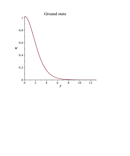
Figure 1: Shown is a numerical approximation to the gound state solution $u(r)$ of (1).

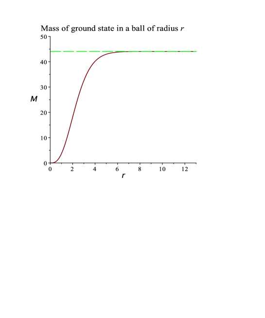
Figure 2: Shown is $M(r):=4\pi\int_{0}^{r}|u(s)|^{2}s^{2}ds$ for the gound state solution $u(r)$ of (1), together with the horizontal asymptote at $14.03\pi\approx\|u\|_{2}^{2}=\lim_{r\to\infty}M(r)$.

Fig. 3, where we display the natural logarithm of $u(r)$ together with a straight line of slope $-1$, appears to suggest a purely exponential decay of the ground state $u(r)$, but appearances are misleading, as visualized in Fig. 4.

     

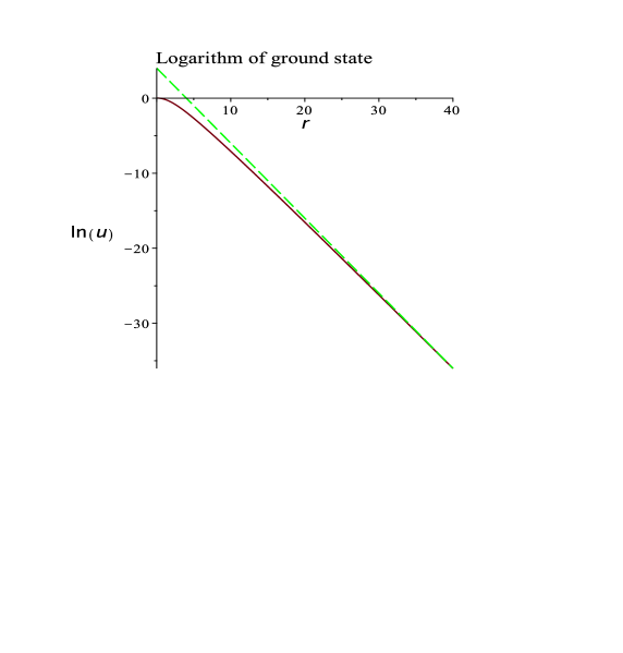
Figure 3: Shown is the natural logarithm of the gound state solution $u(r)$ of (1), together with a straight line of slope $-1$.

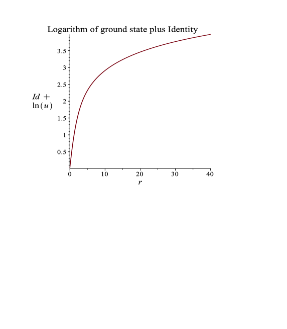
Figure 4: Shown is $r+\ln u(r)$ versus $r$ for the gound state solution $u(r)$ of (1).

Fig. 4 reveals that the map $r\mapsto r+\ln u(r)$ is not asymptotic, for large $r$, to a constant function, which it would be if $u(r)\sim A\exp(-r)$. Instead, this map seems to behave $\propto\ln r$ for large $r$, which is confirmed in Fig. 5.

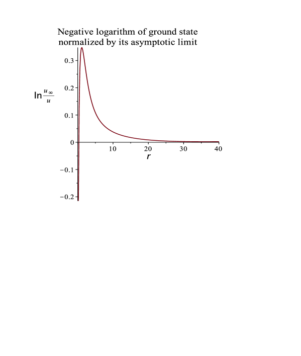
Figure 5: Shown is the negative natural logarithm of the ratio of the gound state solution $u(r)$ of (1) over its asymptotic limit $u_{\infty}(r)=Ar^{\beta}\exp(-r)$ with $\beta\approx 0.754$ and $A\approx 3.37$.

Our numerical computations were carried out with MAPLE’s Cash–Karp fourth-fifth order Runge–Kutta method with degree four interpolant (ck45), which proved more suitable than MAPLE’s default Runge–Kutta–Fehlberg routine rkf45. To overcome the enormous variations over the range of $u(r)$ we solved the ODE for $\ln u(r)$ and asked for 70 digits precision during the computation. The interval halving iterations to determine the correct initial data $u(0)$ and $u^{\prime\prime}(0)$ to yield $\ln u(r)\sim-r$ were terminated after a precision of three significant digits had been achieved, though.

As a test for our results we rescaled the ground state energy $E=E_{0}$ for (4), computed numerically in GW to be $E_{0}=-0.325(74)$, into our units in which the ground state energy $E=-1$. This yields $\|u\|_{2}^{2}=8\pi/\sqrt{|E_{0}|}\approx 44.09$, in good agreement with our result $14.03\pi\approx 44.08$.

IV External $\sim-K/r$ potentials

In its bosonic star interpretation, the Schrödinger–Newton equation (1) captures the quantum-mechanical ground state of a single species of $N$ spin-zero bosons that interact only with Newtonian gravity among themselves, in the Hartree limit $N\to\infty$; cf. Lewin , and see LiebYauCMP for a version with special-relativistic kinetic energy. Since these hypothetical building blocks of the mysterious dark matter will interact gravitationally with other matter, it is of interest to also consider the Schrödinger–Newton equation for bosons which are exposed to an external gravitational potential, which for simplicity we will assume to be radially symmetric and asymptotically $\sim-K/r$ for some $K>0$. Incidentally, equipped with such an additional external $\sim-K/r$ potential the so-generalized Schrödinger–Newton equation also can have bound states if the sign of the self-consistent interaction term (the cubic nonlinearity term at r.h.s.(1)) is changed from “$+$” to “$-$.” Therefore, in this and the next section we consider the equation

$$-\Delta u({\boldsymbol{{s}}})+u({\boldsymbol{{s}}})=\displaystyle{\frac{1}{4\pi}\int_{\mathbb{R}^{3}}\!\!\!\frac{\mathfrak{z}\|u\|_{2}^{2}\mu({\boldsymbol{{s}}}^{\prime})\pm|u|^{2}({\boldsymbol{{s}}}^{\prime})}{\big{|}{\boldsymbol{{s}}}-{\boldsymbol{{s}}}^{\prime}\big{|}}d^{3}\!s^{\prime}}u({\boldsymbol{{s}}})$$ (16)

with $\mathfrak{z}>0$ if the “$+$” sign is chosen, and in this section with $\mathfrak{z}>1$ if the “$-$” sign is; in the next section we also allow $\mathfrak{z}\geqslant 0.825$. Here, $\mu({\boldsymbol{{s}}})\geqslant 0$ is a given probability measure, in the following assumed to be radially symmetric. Eq.(16) with the “$-$” sign and $\mathfrak{z}>1$ captures the ground state of a positive ion with hypothetical bosonic “electrons” in the Hartree limit $N\to\infty$, BenguriaLieb , LiebSeiringer ; cf. also BEGMY , FKS , P , KieJMP , LNR , Rou , and references therein. In that case $\mu({\boldsymbol{{s}}})$ represents the (normalized) charge distribution of the nucleus, which usually is modelled by a Dirac $\delta$ measure but may also be considered to be bounded and radially symmetric decreasing. In the gravitational interpretation (i.e. “$+$” sign in (16)), $\mu({\boldsymbol{{s}}})$ is the normalized mass distribution of the other matter.

Eq.(16), with either sign, is the formal Euler–Lagrange equation for the minimization of the functional

$${\mathfrak{F}}^{\mp}(u):=\int_{\mathbb{R}^{3}}\left(\big{|}\nabla u\big{|}^{2}+|u|^{2}\right)\!({\boldsymbol{{s}}})\,d^{3}\!s\mp\frac{1}{8\pi}\int_{\mathbb{R}^{3}}\int_{\mathbb{R}^{3}}\frac{|u|^{2}({\boldsymbol{{s}}})|u|^{2}({\boldsymbol{{s}}}^{\prime})}{\big{|}{\boldsymbol{{s}}}-{\boldsymbol{{s}}}^{\prime}\big{|}}d^{3}\!sd^{3}\!s^{\prime}-\mathfrak{z}\frac{\|u\|_{2}^{2}}{4\pi}\int_{\mathbb{R}^{3}}\int_{\mathbb{R}^{3}}\frac{|u|^{2}({\boldsymbol{{s}}})\mu({\boldsymbol{{s}}}^{\prime})}{\big{|}{\boldsymbol{{s}}}-{\boldsymbol{{s}}}^{\prime}\big{|}}d^{3}\!s^{\prime}d^{3}\!s$$ (17)

     

over the set of $u\in H^{1}(\mathbb{R}^{3})$ under the Nehari condition that $u\neq 0$ satisfies ${4\pi}\int_{\mathbb{R}^{3}}\big{(}\big{|}\nabla u\big{|}^{2}({\boldsymbol{{s}}})+|u|^{2}({\boldsymbol{{s}}})\big{)}d^{3}s=\int_{\mathbb{R}^{3}}\int_{\mathbb{R}^{3}}{\big{|}{\boldsymbol{{s}}}-{\boldsymbol{{s}}}^{\prime}\big{|}}^{-1}{|u|^{2}({\boldsymbol{{s}}})\big{[}\mathfrak{z}\|u\|_{2}^{2}\mu({\boldsymbol{{s}}}^{\prime})\pm|u|^{2}({\boldsymbol{{s}}}^{\prime})\big{]}}d^{3}sd^{3}s^{\prime}$; no normalization condition on $\int|u|^{2}({\boldsymbol{{s}}})d^{3}s$ is imposed. Under our assumptions that $\mathfrak{z}>0$ if the upper sign is chosen, and $\mathfrak{z}>1$ if the lower one is, we may expect that a unique positive minimizer of ${\mathfrak{F}}^{\mp}(u)$ exists and satisfies (16), and in the following we assume this; cf. KK .

The asymptotic behavior of such a positive solution of (16) for rapidly decreasing $\mu(r)$ (bounded by a Schwartz function) can be obtained by adapting the strategy of V. Moroz and J. van Schaftingen MvS to (16). We find

$$\lim_{r\to\infty}r^{1-(\mathfrak{z}\pm 1)\|u\|_{2}^{2}/8\pi}e^{r}u(r)\in(0,\infty);\vspace{-10pt}$$ (18)

thus, $u(r)=Ae^{-r}/r^{1-(\mathfrak{z}\pm 1)\|u\|_{2}^{2}/8\pi}+$l.o.t. for an $A>0$.

V Concluding remarks

In section IV we have only considered the Schrödinger–Newton and Hartree equations in settings which allow a straightforward adaptation of the strategy of MvS . In the ionic Hartree problem with $\mu({\boldsymbol{{s}}})=\delta({\boldsymbol{{s}}})$, it is known that a minimizer exists also for $\mathfrak{z}_{*}\leqslant\mathfrak{z}\leqslant 1$ with $\mathfrak{z}_{*}\approx 0.825$; cf.BenguriaLieb , LiebSeiringer , Baum . Although we did not investigate this more difficult neutral atom and negative ion regime to the point that we can make a definite statement, our preliminary inquiry leads us to the surmise that (18) continues to hold for neutral bosonic atoms and negative ions, so that in this regime one seems to have $u(r)\sim Ae^{-r}\!/r^{\gamma}$ with $\!\gamma\geqslant 1$. Interestingly, (18) thus suggests that the asymptotic form of $u(r)$ proposed by K. P. Tod and I. Moroz in TM for (1) is instead true for the Hartree ground state of a neutral bosonic atom in the $N\to\infty$ limit, when $\mathfrak{z}=1$. In all the cases discussed in section IV the asymptotic form $u(r)\sim Ae^{-r}/r^{\gamma}$ holds with $\gamma<1$.

Given that the question of the asymptotic decay of the Schrödinger–Newton ground state has received several conflicting answers until rigorous results showed the way, it is desirable to rigorously vindicate also the findings and the surmise reported in sections IV and V.

References

miki@math.rutgers.edu

References

• (1) S.I. Pekar, Untersuchungen über die Elektronentheorie der Kristalle, Akademie Verlag, Berlin (1954).
• (2) H. Fröhlich, “Theory of electrical breakdown in ionic crystals,” Proc. Roy. Soc. Ser. A 160, 230–241 (1937).
• (3) H. Fröhlich, “Electrons in lattice fields,” Adv. in Phys. 3, 325–361 (1954).
• (4) M. D. Donsker and S. R. S. Varadhan, “The polaron problem and large deviations,” Phys. Rep. 77, 235–237 (1981).
• (5) M. D. Donsker and S. R. S. Varadhan, “Asymptotics for the polaron,” Commun. Pure Appl. Math. 36, 505–528 (1983).
• (6) E. H. Lieb and L. E. Thomas, “Exact ground state energy of the strong-coupling polaron,” Commun. Math. Phys. 183, 511–519 (1997).
• (7) E. H. Lieb, “Existence and uniqueness of the minimizing solution of Choquard’s nonlinear equation,” Studies Appl. Math. 57, 93–105 (1977).
• (8) Ph. Choquard, J. Stubbe, and M. Vuffray, “Stationary solutions of the Schrödinger–Newton model — An ODE approach,” Diff. Int. Eq. 21, 665–679 (2008).
• (9) R. Penrose, “On gravity’s role in quantum state reduction,” Gen. Rel. Grav. 28, 581–600 (1996).
• (10) M. Lewin, “Derivation of Hartree’s theory for mean-field Bose gases,” Journées équations aux dérivées partielles, Exposé no. 7, 21pp. (2013).
• (11) V. Moroz and J. van Schaftingen, “A guide to the Choquard equation,” J. Fixed Point Th. Appl. 19, 773–813 (2017).
• (12) D. Kumar and V. Soni, “Single particle Schrödinger–Newton equation with gravitational self-interaction,” Phys. Lett. A 271, 157–166 (2000).
• (13) K. P. Tod, “The ground state energy of the Schrödinger–Newton equation,” Phys. Lett. A 280, 173–176 (2001).
• (14) K. P. Tod, and I. Moroz, “An analytical approach to the Schrödinger–Newton equations,” Nonlinearity 12, 201–216 (1999).
• (15) I. Moroz, R. Penrose, and K. P. Tod, “Spherically symmetric solutions of the Schrödinger–Newton equations,” Class. Quant. Grav. 15, 2733–2742 (1998).
• (16) R. Harrison, “A numerical study of the Schrödinger–Newton equations,” Ph.D. thesis, Dept. Math., Univ. Oxford (2001).
• (17) V. Moroz and J. van Schaftingen, “Ground states of nonlinear Choquard equations: existence, qualitative properties, and decay asymptotics,” J. Funct. Anal. 265, 153–184 (2013).
• (18) D. Greiner and G. Wunner, “Quantum defect analysis of the eigenvalue spectrum of the Newton–Schrödinger equation,” Phys. Rev. A 74, 052106 5pp. (2006).
• (19) E. H. Lieb and H.-T. Yau, “The Chandrasekhar theory of stellar collapse as the limit of quantum mechanics,” Commun. Math. Phys. 112, 147–174 (1987).
• (20) R. Benguria and E. H. Lieb, “Proof of stability of highly negative ions in the absence of the Pauli principle,” Phys. Rev. Lett. 50, 1771–1774 (1983).
• (21) E. H. Lieb and R. Seiringer, The stability of matter in quantum mechanics, 1st ed. (Cambridge University Press, Cambridge, UK 2010)
• (22) C. Bardos, L. Erdős, F. Golse, N. Mauser, and H.-T. Yau, “Derivation of the Schrödinger–Poisson equation from the quantum $N$-body problem,” C. R. Acad. Sci. Paris 334, 515–520 (2002).
• (23) J. M. Fröhlich, A. Knowles, and S. Schwarz, “On the mean-field limit of bosons with Coulomb two-body interaction,” Commun. Math. Phys. 288, 1023–1059 (2009).
• (24) P. Pickl, “A simple derivation of mean-field limits for quantum systems,” Lett. Math. Phys. 97, 151–164 (2011).
• (25) M. K.-H. Kiessling, “The Hartree limit of Born’s ensemble for the ground state of a bosonic atom or ion,” J. Math. Phys. 53, 095223 21pp. (2012).
• (26) M. Lewin, P.T. Nam, and N. Rougerie, “Derivation of Hartree’s theory for generic mean-field Bose systems,” Adv. Math. 254, 570–621 (2014).
• (27) N. Rougerie, “De Finetti theorems, mean-field limits and Bose-Einstein condensation,” arXiv:1506.05263v2 [math-ph] (2020).
• (28) B. Kawohl and S. Krömer, “Uniqueness and symmetry of minimizers of Hartree type equations with external Coulomb potential,” Adv. Calc. Var. 5, 427–432 (2012).
• (29) B. Baumgartner, “On the Thomas–Fermi–von Weizsäcker and Hartree energies as functions of the degree of ionization,” J. Phys. A17, 1593–1602 (1984).