One vs Previous and Similar Classes Learning - A Comparative Study

Daniel Cauchi
Faculty of Information
& Communication Technology
University of Malta
Msida, MSD 2080
daniel.cauchi.17@um.edu.mt
Adrian Muscat
Faculty of Information
& Communication Technology
University of Malta
Msida, MSD 2080
adrian.muscat@um.edu.mt

Abstract

When dealing with multi-class classification problems, it is common practice to build a model consisting of a series of binary classifiers using a learning paradigm which dictates how the classifiers are built and combined to discriminate between the individual classes. As new data enters the system and the model needs updating, these models would often need to be retrained from scratch. This work proposes three learning paradigms which allow trained models to be updated without the need of retraining from scratch. A comparative analysis is performed to evaluate them against a baseline. Results show that the proposed paradigms are faster than the baseline at updating, with two of them being faster at training from scratch as well, especially on larger datasets, while retaining a comparable classification performance.

1 Introduction

For multi-class classification problems [1], models are often built using a series of binary classifiers. The model uses a protocol to build the binary classifiers during training so it is then able to perform prediction using the built classifiers and the previously mentioned protocol. In this work, this protocol is referred to as the learning paradigm, or just paradigm. Examples of existing paradigms are One vs Rest (OvR) [2] and One vs One (OvO), also known as Round Robin Rule Learning [3, 1]. This work proposes three paradigms. The first, Similar Classes Learning (SCL), is a modified version of the paradigm proposed by [4]. One vs Previous (OvP) is a new paradigm and One vs Previous Similar Classes (OvPSC) is a combination of the previous two.

Existing paradigms are usually highly computationally demanding [5, 6] and if a model built with these paradigms needs to be updated with new data, it often needs to be retrained from scratch. Each of the proposed paradigms decouple the classifiers of the model in some way, such that, as new data enters the system, only relevant parts of the model need to be modified. This gives them application in Lifelong Machine Learning [7, 8].

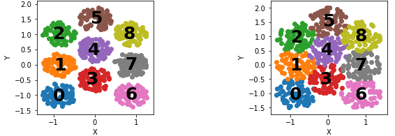
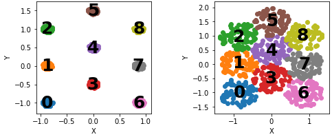
Two datasets are used to evaluate the paradigms against a baseline. The first is a real-world dataset of spatial relations in images, SpatialVOC2K [9, 10, 11]. The second is a synthetic dataset consisting of nine clusters, which can be seen in Figure 1, used to experiment freely with its characteristics.

Refer to caption — Figure 1: The synthetic clusters datasets with radius=0.4 (left) and radius=0.525 (right). Each number corresponds to a class label.

The contribution of this paper are the following: a) propose the three paradigms, one of which is a modification of a known method, one is new and one which is a combination of the previous two b) conduct a comparative analysis against a bassline and evaluate them on their computational time and classification performance, using two datasets, one of which is synthetic and the other is from a real world scenario.

2 Related Work

This section provides an overview of contributions related to this work and how the proposed paradigms differ from the existing alternatives.

One of the standard paradigms is One vs Rest (OvR) [2]. Here, each class is trained against all other classes resulting in as many classifiers as classes. For prediction, an argmax function is used to determine the output class. The nature of this paradigm is simple but is of a brute force nature. While the proposed paradigms share some similarities with this paradigm, they also differ in such a way that simplicity is traded for efficiency. Certain other paradigms claim to be have better classification performance, however the evidence suggesting this is usually not sufficient or results may be biased [2]. Hence why OvR remains commonplace and is the reason it is used as a baseline paradigm for this work.

A standard alternative to OvR is One vs One (OvO) [1, 3], where every class is trained every other class in pairs, resulting in a model characterized by $\frac{n(n-1)}{2}$ classifiers. In the prediction phase, a scoring method is used and the class with the most winning classifiers is chosen. The prediction algorithm treats the classifier output as binary, without considering the score. This is unlike OvR which compares the score of each classifier to determine the output. Both OvP and OvPSC treat the classifier output as binary as well.

[12] uses a one class SVM for each class, allowing the classifiers for each class to be decoupled from the data of other classes. This allows the model to mitigate disruption when new classes are introduced; a concept called Cumulative Learning, which is a sub-area of Lifelong Machine Learning [7].

Cumulative learning is also used by [4]. With this method, as a new class comes in, it is trained against its similar classes only, while the classifiers for the similar classes are retrained to include the new class in their negative set. [4]. SCL uses a similar algorithm, however, significant additions were made to generalize the model such that it can be used by any multi-class model that uses a series of binary classifiers. On the other hand, [4] solves the problem of Open World Classification [13], where the classes in the test set are not assumed to have all been seen during training.

3 The Paradigms

This section is dedicated to discussing the individual paradigms. Each paradigm consists of two algorithms: the training algorithm and the prediction algorithm. Before starting with the algorithms themselves, the term similarity, and by extension similar classes, is defined, which are used by SCL and OvPSC. The definition provided by [4] is used:

Definition 3.1

Similar Classes (SC): Given an existing model at iteration $t$ with classifiers ${C_{1},C_{2},...,C_{t}}$ for classes ${c_{1},c_{2},...,c_{t}}$ respectively, when at iteration $t+1$ , the $N_{t+1}$ examples for class $c_{t+1}$ enter the system, these are run through each classifier of the past classes and if a percentage $\lambda_{sim}$ of these examples are classified as positive for a classifier, then the new class and the class corresponding to that classifier are said to be similar.

$\lambda_{sim}$ is a hyperparameter. For the experiments, this was set to a constant 2%, which was the value used in [4] and through preliminary testing, this value was also found to work best for the used datasets. If it is taken to be lower, then too many classes are marked as similar, reducing the efficiency of the paradigms and by extension the models created by them. If it is taken to be higher, then not enough classes are marked as similar, leading to a decline in classification performance.

With regards to algorithm notation, data types are underlined, keywords are in bold text, # in front of a list or set represents its size, lists are ordered and are represented within [] while sets are unordered and are represented within {}.

3.1 Similar Classes Learning (SCL)

This paradigm is a modification on [4]. The modifications allow it to solve a standard multi-class classification problem.

Input: Sets of Training Examples

E_{1},E_{2},\ldots{},E_{m}

for Classes

c_{1},c_{2},\ldots{},c_{m}

Base Classifier B
float

\lambda_{sim}

Model M = [ ]

foreach int i in [1…m] do

Set of classes

SC_{i}=\{\}

Set of classes

CannotBe_{i}=\{\}

foreach Classifier $C_{j}$ in M do

int count = 0

foreach Training Example e in $E_{i}$ do

if $C_{j}$ classifies e as positive then

count = count + 1

if count $>\lambda_{sim}*\#E_{i}$ then

SC_{i}=SC_{i}\cup c_{j}

SC_{j}=SC_{j}\cup c_{i}

Retrain

C_{j}

with

c_{j}

as the positive class and

SC_{j}

as the negative classes

else

CannotBe_{j}=CannotBe_{j}\cup c_{i}

if SC is empty then

C_{i}

= DummyClassifier

else

Train

C_{i}

of type B with

c_{i}

as the positive class and

SC_{i}

as the negative classes

Append

C_{i}

to M

Algorithm 1 SCL Training

When training (Algorithm 1), the inputs are the training examples for each class and a base classifier. These inputs are the same as for that of OvR. The base classifier can be any binary classifier, such as a logistic regressor or support vector machine. The choice of classifier will affect how the decision boundaries are built. The last input is $\lambda_{sim}$ discussed previously.

Starting from an empty model, the algorithm iterates over each class, initializing an empty Similar Classes (SC) set and CannotBe set (lines 1 - 4). The reasoning behind CannotBe is: if all the examples of a class B, save for a few outliers, have been classified as negative by a classifier for a class A, then if another example is introduced to the system and the classifier for class A has classified it as positive, then it cannot be, or at least it is highly unlikely, that it belongs to class B. This CannotBe variable is what distinguishes this work from [4] and is what allows the paradigm to be used for the Closed World Assumption [13], where every class in the testing data is assumed to have been seen during training. Using the examples of the current class, the algorithm finds the SC of this class using existing classifiers (lines 5 - 10), adds each class to the SC of the other class symmetrically (lines 11-12) and retrains the classifier of the existing class with its previous negative examples and the new class as the negative set (line 13). Otherwise the current class is added to the CannotBe set of the existing class (lines 14 - 15). If a class is not similar to any other class, it is given a dummy classifier which gives the highest positive score to any example during prediction (lines 16 - 17). In contrast, if similar classes are found, the class is given a classifier which is trained with its similar classes as the negative set (lines 18 - 19). Lastly, this new classifier is appended to model (line 20).

Input: Example to be classified e
Model M = [

C1,C2,\ldots{},C_{m}

]
List of set of classes

[CannotBe_{1},CannotBe_{2},\ldots{},CannotBe_{m}]

TopClass = NULL

BiggestConfidence = -

\inf

CannotBe = {}

foreach int i in [1…m] do

if $c_{i}$ not in CannotBe then

float conf = Confidence in e given by

C_{i}

if conf > BiggestConfidence then

BiggestConfidence = conf

TopClass =

c_{i}

if conf > 0 then

CannotBe=CannotBe\cup CannotBe_{i}

return TopClass

Algorithm 2 SCL Prediction

As inputs for prediction (Algorithm 2), besides the example to be predicted, the algorithm needs to know the CannotBe set of each class. A local CannotBe set is kept (line 3). The algorithm iterates over all the binary classifiers of the model in the order in which they were built, skipping over ones which are in the local CannotBe set (lines 4 - 5). If a class gives a positive confidence score, the local CannotBe set is unionized with the CannotBe of the class (lines 10 - 11). Finally, it predicts the class whose classifier gives the highest confidence (lines 7 - 9, 12).

One may notice that the order in which the classes enter the system matters. A different order will lead to a different model and may affect classification performance. This observation applies to all three of the proposed paradigms and finding the optimal order is still an open question. Besides training the model, SCL and OvPSC also need to spend time searching for the similar classes during training, hence, training time also depends on the prediction speed of the base classifier used. In all the proposed paradigms, if new examples belonging to a new class come in, there is no need to retrain the entire model from scratch, similar to OvO, but unlike OvR. Unlike OvO, however, there is no need to train as many new classifiers as there are classes, but only train a single new classifier. In the worst case, when all classes are similar, the decision boundary of this paradigm will be identical to that of OvR.

3.2 One vs Previous (OvP)

The next paradigm, One vs Previous (OvP), is new. In short, this starts from a dummy classifier and proceeds to make each subsequent classifier more and more specific.

Input: Sets of Training Examples

E_{1},E_{2},...E_{m}

for Classes

c_{1},c_{2},...c_{m}

Base Classifier

Model M = [ ]

foreach int i in [1…m] do

if i = 1 then

Classifier

C_{i}

= DummyClassifier

else

Train

C_{i}

of type B with

c_{i}

as the positive class and

c_{1}...c_{i-1}

as the negative classes

Append

C_{i}

to M

Algorithm 3 OvP Training

The inputs for the training algorithm (Algorithm 3) consist of the examples and base classifier. A dummy classifier is created for the first class (line 4). Subsequent classes are given a classifier which is trained using the examples of classes which already have a classifier built for them (the previous classes) as the negative examples (lines 5 - 6).

Input: Example to be classified e
Model M = [

C1,C2,...,C_{m}

]

foreach int i in [m…1] do

float conf = Confidence in e given by

C_{i}

if conf >0 then

return

c_{i}

Algorithm 4 OvP Prediction

The prediction algorithm (Algorithm 4), iterates through the classifiers in the reverse order of which they were built and predicts the first class whose classifier gives a positive confidence.

When training, the classifiers do not depend on each other. Thus, similar to OvR but unlike SCL and OvPSC, training the individual classifiers can be parallelized.

3.3 One vs Previous Similar Classes (OvPSC)

This final paradigm is a combination of the previous two, where it builds the classifiers similar to SCL, without retraining, and then during prediction it uses a local CannotBe to see which classes it should not consider, then performs an OvP prediction over the remaining classes.

Input: Sets of Training Examples

E_{1},E_{2},...E_{m}

for Classes

c_{1},c_{2},...c_{m}

Base Classifier B
float

\lambda_{sim}

Model M = [ ]

foreach int i in [1…m] do

Set of classes

SC_{i}=\{\}

Set of classes

CannotBe_{i}=\{\}

if i == 1 then

Classifier

C_{i}

= DummyClassifier

else

foreach $C_{j}$ in M do

int count = 0

foreach Training Example e in $E_{i}$ do

if $C_{j}$ classifies e as positive then

count = count + 1

if count $>\lambda_{sim}*\#E_{i}$ then

SC_{i}=SC_{i}\cup c_{j}

else

CannotBe_{j}=CannotBe_{j}\cup c_{i}

Train

C_{i}

of type B with

c_{i}

as the positive class and

SC_{i}

as the negative classes

Append

C_{i}

to M

Algorithm 5 OvPSC Training

The training algorithm (Algorithm 5) has the same inputs as SBL. Starting from an empty model, the algorithm iterates over all the classes, giving each one its own SC and CannotBe set (lines 1 - 4). The first class is given a dummy classifier (lines 5 - 6). Iterating through existing classifiers, the classes which are similar to the class in consideration are found and added to the SC of this class, however, as opposed to SBL, the relationship is not symmetric (lines 7 - 14). If the current class is not similar to the existing class, it is added to the CannotBe of the existing class (lines 15 - 16). Lastly, a classifier is trained for the current class against its similar classes, without any modification of existing classifiers, which is then appended to the model (lines 17 - 18).

Input: Example to be classified e
Model M = [

C1,C2,...,C_{m}

]
List of set of classes

[CannotBe_{1},CannotBe_{2},...,CannotBe_{m}]

CannotBe = {}

Class toReturn = NULL

foreach int i in [1…m] do

if $c_{i}$ not in CannotBe then

float conf = Confidence in e given by

C_{i}

if conf >0 then

CannotBe=CannotBe\cup CannotBe_{i}

toReturn =

c_{i}

return toReturn

Algorithm 6 OvPSC Prediction

For prediction, (Algorithm 6, the algorithm keeps a local CannotBe and iterates over the classes in the order of which the classifiers were built (lines 1 - 3). If a class is in the local CannotBe, it is skipped (line 4). Otherwise, if the classifier returns a positive confidence, the CannotBe of that class is unionized with the local CannotBe and the algorithm will return the current class if no other class gives a positive confidence (lines 5 - 9).

One may notice that since the first class is given a dummy classifier, it will always be similar to every other class. In the worst case, when all classes are similar, the decision boundary of this paradigm will be identical to that of OvP.

4 Datasets

4.1 SpatialVOC2K

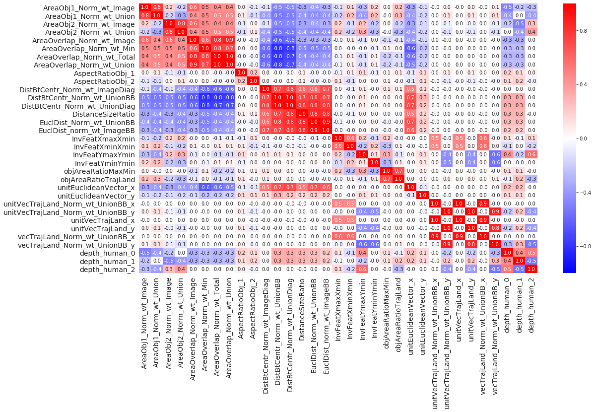
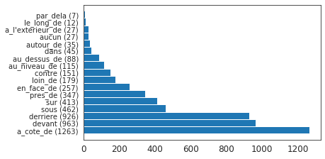
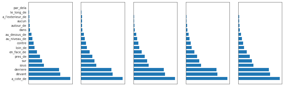
The first dataset used is one containing spatial relations in images [9, 10, 11], consisting of 20 different objects and 17 different target values. It is split into two parts, of which the entitled best part is used, containing 5317 examples, further subdivided into five stratified folds. Each feature vector contains language and geometric features. From preliminary testing and manual feature selection, the one-hot vector for the language features was chosen and the initial 34 geometric features, which extend to 37 once the feature rel_position is expanded into a one-hot vector, were reduced to 23 features. For the full list of features and additional visualisations of this dataset, see Appendix A.

4.2 Synthetic Clusters

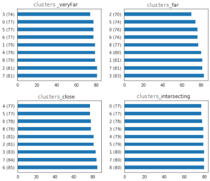
The second dataset consists of 9 circular clusters on a 2D plane of up to 100 points each as can be seen in Figure 1. This dataset was created for free experimentation with its characteristics. Four variants of this dataset were created, each with a varying radius: clusters_veryFar has radius 0.1, clusters_far has radius 0.4, clusters_close has radius 0.5 and clusters_intersecting has radius 0.525. At radius 0.5, the clusters are touching. For additional details and visualisations about this dataset see Appendix 5.

5 Experiments

A numer of experiments were devised to show how the paradigms perform in different scenarios. With regards to base classifiers, a logistic regressor with the liblinear solver [14] and an SVM with RBF Kernel [15, 16] were used.

The training pipeline is as follows. First, the datasets are split into five stratified folds. The non-one-hot features of this dataset are also normalized to mean 0 and standard deviation 1. The parameters for normalization are obtained on the train set and then applied to the test set. There are thus five runs, one for each fold. Before training in each run, a grid search is performed over the C parameter of both classifiers, where C ranges from 0.0001 to 100 using a logarithmic scale. Lastly, the best classifier is trained over the entire train set and evaluated over the test set. In each experiment, the classes enter the system in order of frequency, starting from the most frequent first, because in a practical scenario this would usually be the order in which classes would appear.

5.1 Experiment 1

In the first three experiments, 1a, 1b and 1c, after splitting into the test and train sets, the train set is further split into three stratified parts which are called M0, M1 and M2. The first M-set, M0, contains 50% of the data, M1 contains 30% of the data and M2 contains the last 20%. These proportions were chosen such that they represent a practical scenario, starting with most data at the start, then slowly decreasing. The experiment then simulates what happens when each M-set enters the system one after the other, M0 to M2, and the models are updated in accordance with the new data. The strategy for updating is what varies between the experiments. The hyperparameters for these experiments are tuned only once on the first M set, then kept constant for all the classifiers till the end of the run, as this was observed to work best for these datasets. Lastly, for experiments 1b and 1c, with regards to the SCL and OvPSC paradigms, once similar classes are determined using the first M-set, they are kept the same for the subsequent M-sets.

5.1.1 Experiment 1a - Retraining from scratch

For this first experiment, the model is retrained from scratch with the accumulated data as each M-set enters the system. This means that in the first iteration, it is trained with the data in M0, then when M1 enters, the weights are reset and the model is retrained with the data in both M0 and M1. The same happens for the final M-set.

5.1.2 Experiment 1b - Fine-tune with new set

In this experiment, when the second and third set come in, the weights are retained from the previous iteration and the model is trained until convergence using the new set only.

5.1.3 Experiment 1c - Fine-tune with entire set

This last experiment entails retaining the weights from previous iterations when a new set comes in and retraining with the data in both the previous and new M-set until convergence. This transferring of weights for updating used in both experiment 1b and experiment 1c is often called transfer learning [17].

5.2 Experiment 2

The second experiment evaluates the models when the number of classes N changes. The train set is first split into N sets, where each set contains all the examples of a single class. Hyperparameter tuning is done each time a new class enters the system, and any classifiers which need to be trained or retrained will use these new hyperparameters, leading to different classifiers having different hyperparameters. While OvR is retrained from scratch each time a new class enters the system, the other classifiers are updated as discussed in their respective chapters in Section 3. When showing the prediction results at each iteration, only the examples for classes that the model has already seen are used.

6 Results and Discussion

In this section the results obtained from the experiments are shown and discussed. The F1-scores for the clusters datasets is always almost identical to the accuracy, since the classes for these datasets are equally distributed, therefore these will not be shown. Time for the clusters datasets will only be shown for one variant as these ended up being very similar. With regards to experiments 1b and 1c, the results for M=0 is the same as that of 1a, hence they are not shown again. The full tables, however, are given in the Appendix C.

Table 1: Experiment 1a - Retraining from scratch

			OvR LR	SCL LR	OvP LR	OvPSC LR	OvR SVM	SCL SVM	OvP SVM	OvPSC SVM
SpatialVOC2K	M=0	accuracy	0.542	0.483	0.538	0.540	0.541	0.540	0.544	0.552
		f1	0.337	0.343	0.289	0.312	0.340	0.349	0.302	0.310
		time	0.268	1.422	0.281	0.614	1.706	10.258	0.935	1.369
	M=1	accuracy	0.549	0.533	0.547	0.549	0.561	0.528	0.553	0.559
		f1	0.347	0.371	0.303	0.316	0.360	0.360	0.306	0.316
		time	0.429	2.332	0.435	0.980	4.233	25.382	2.195	2.820
	M=2	accuracy	0.548	0.542	0.554	0.555	0.567	0.526	0.564	0.567
		f1	0.351	0.367	0.316	0.327	0.365	0.363	0.327	0.317
		time	0.545	2.973	0.544	1.227	6.506	40.824	3.338	4.100
clusters_veryFar	M=0	accuracy	1.000	0.660	0.783	0.867	1.000	1.000	1.000	1.000
	M=0	time	0.024	0.147	0.035	0.104	0.028	0.163	0.035	0.119
	M=1	accuracy	1.000	0.660	0.783	0.761	1.000	1.000	1.000	1.000
	M=1	time	0.028	0.206	0.038	0.148	0.039	0.233	0.038	0.172
	M=2	accuracy	1.000	0.660	0.783	0.673	1.000	1.000	1.000	1.000
	M=2	time	0.029	0.244	0.039	0.177	0.050	0.279	0.039	0.208
clusters_far	M=0	accuracy	0.978	0.745	0.918	0.920	0.991	0.999	0.996	0.996
	M=1	accuracy	0.983	0.712	0.925	0.925	0.988	0.999	1.000	1.000
	M=2	accuracy	0.984	0.702	0.928	0.930	0.980	1.000	1.000	1.000

Table 2: Experiment 1b - Fine-tune with new set only

			OvR LR	SCL LR	OvP LR	OvPSC LR	OvR SVM	SCL SVM	OvP SVM	OvPSC SVM
SpatialVOC2K	M=1	accuracy	0.532	0.470	0.531	0.527	0.530	0.518	0.528	0.540
		f1	0.292	0.304	0.282	0.288	0.315	0.303	0.286	0.290
		time	0.162	1.051	0.192	0.130	0.658	5.706	0.395	0.291
	M=2	accuracy	0.528	0.456	0.524	0.520	0.520	0.515	0.521	0.531
		f1	0.286	0.287	0.274	0.287	0.302	0.291	0.284	0.276
		time	0.111	0.740	0.136	0.091	0.327	2.740	0.219	0.154
clusters_far	M=1	accuracy	0.980	0.669	0.918	0.918	0.977	0.984	1.000	0.999
	M=1	time	0.020	0.076	0.032	0.017	0.020	0.070	0.032	0.016
	M=2	accuracy	0.977	0.682	0.918	0.907	0.955	0.994	0.993	0.980
	M=2	time	0.018	0.074	0.032	0.016	0.019	0.066	0.031	0.016

Table 3: Experiment 1c - Fine-tune with entire dataset

			OvR LR	SCL LR	OvP LR	OvPSC LR	OvR SVM	SCL SVM	OvP SVM	OvPSC SVM
SpatialVOC2K	M=1	accuracy	0.549	0.486	0.547	0.548	0.561	0.556	0.553	0.559
		f1	0.347	0.365	0.303	0.313	0.360	0.358	0.306	0.312
		time	0.423	2.685	0.432	0.341	4.379	37.415	2.181	1.698
	M=2	accuracy	0.548	0.485	0.554	0.555	0.567	0.561	0.564	0.567
		f1	0.351	0.355	0.316	0.326	0.365	0.365	0.327	0.314
		time	0.541	3.263	0.542	0.431	6.702	58.650	3.308	2.557
clusters_far	M=1	accuracy	0.983	0.712	0.925	0.925	0.988	0.997	1.000	0.987
	M=1	time	0.025	0.088	0.036	0.019	0.032	0.085	0.035	0.019
	M=2	accuracy	0.984	0.702	0.928	0.928	0.980	0.997	1.000	0.983
	M=2	time	0.027	0.093	0.038	0.020	0.038	0.092	0.038	0.020

Table 4: Experiment 2 - Retrain with new class - SpatialVOC2K - Last Class

		OvR LR	SCL LR	OvP LR	OvPSC LR	OvR SVM	SCL SVM	OvP SVM	OvPSC SVM
N17=par_dela	accuracy	0.547	0.537	0.553	0.554	0.573	0.442	0.564	0.563
	f1	0.351	0.341	0.310	0.308	0.348	0.191	0.303	0.299
	time	0.640	0.090	0.011	0.022	5.695	0.909	0.010	0.026

Table 5: Experiment 2 - Retrain with new class - clusters_far - Last class

		OvR LR	SCL LR	OvP LR	OvPSC LR	OvR SVM	SCL SVM	OvP SVM	OvPSC SVM
N9=2	accuracy	0.981	0.689	0.914	0.921	0.997	0.588	0.906	0.816
	f1	0.982	0.691	0.910	0.918	0.997	0.488	0.881	0.746
	time	0.029	0.048	0.002	0.038	0.038	0.057	0.003	0.047

6.1 Experiment 1

6.1.1 Experiment 1a - Retraining from scratch

Table 1 shows that Logistic Regression, in terms of classification performance, performs worse on the clusters datasets when compared to SVM, as this dataset is not-linearly separable. Meanwhile, it performs only slightly worse on SpatialVOC2K, indicating that the features of this dataset make it more linearly separable. Almost every classifier gets better classification performance as the dataset size increases, that is, as M increases. Subsequently, it also takes more time to train. As expected, LR also takes less time to train than the corresponding SVM models, when the paradigm is kept constant.

The three proposed paradigms are comparable to the baseline in classification performance, in some cases being slightly better. That said, OvR is still usually better, albeit with a small difference ranging from 1%-5%. SCL-LR when used on the clusters dataset, however, performs poorly with regards to classification performance. This can be seen in the clusters_veryFar dataset results. With regards to the F1 score on SpatialVOC2K, the most comparable to OvR is the SCL paradigm, while OvP and OvPSC perform around 4-5% worse. Meanwhile, OvP and OvPSC accuracy is comparable to that of OvR, with less than 1% difference.

With regards to time, SCL always takes the longest when given the entire dataset as a whole, due to the retraining this paradigm performs. Focusing on the SVM variants, OvP is always the one which takes the least time, taking half the time of OvR. This takes less time than OvPSC, even though the latter uses less training examples, due to OvP not needing to check for similar classes, which is an indication that this checking contributes a significant overhead. OvR is faster than OvPSC on the clusters datasets, further solidifying the fact that this overhead is significant. However, on SpatialVOC2K OvPSC is faster than OvR, which indicates that OvPSC scales better on bigger datasets, as the overhead becomes less significant.

6.1.2 Experiment 1b - Fine-tune with new set

In this experiment, SCL-LR also performs poorly on the clusters datasets (Table 2). In terms of the Logistic Regression models, OvR is the best performing paradigm on the clusters Datasets. Since there is less data in each M-set, training time for all models takes less each time, indicating that the models do not take longer to converge if different data is used. Furthermore, OvPSC takes less time than OvR in this case, because it does not need to search for similar classes again. When considering the SVM models, in most cases, at least one of the models built with one of the proposed paradigms either outperforms, is equal to or comes very close to OvR with regards to classification performance on SpatialVOC2K, while the time taken to train is much less. When all M-sets enter the system, almost no classifier performed better than that in experiment 1a, indicating that for these datasets, fine-tuning with the new set only might not be as effective in retaining classification performance. However, if time has a higher priority, one will have to consider the trade-off, especially on much larger datasets.

6.1.3 Experiment 1c - Fine-tune with entire dataset

After conducting this experiment, with regards to time, OvR and OvP remain mostly unaffected, while OvPSC takes less time. On the other hand, the SCL-SVM model, takes much longer on SpatialVOC2K as M increases but ends up improving its classification performance over experiment 1a. Classification performance for the other models is mostly unaffected. No significant difference was observed on the clusters datasets.

6.2 Experiment 2

In this section, the results after training for the final class are shown in Tables 4 and 5 for SpatialVOC2K and the clusters_far dataset respectively. It can be observed that, for SpatialVOC2K especially, timing to add a new class decreases remarkably when using one of the proposed paradigms, since they do not retrain from scratch. Classification performance for the Logistic Regression models are retained when compared to previous experiments. While OvR retains its classification performance when using SVM on the clusters dataset due to retraining from scratch, the other methods perform worse when using different hyperparameters for different classifiers on this dataset. When comparing the SVM variants on SpatialVOC2K, while SCL performs worse when changing hyperparameters between classifiers, classification performance for OvP and OvPSC is mostly retained, with about 1% less accuracy and 5% less F1-score.

7 Conclusion

This work proposed three paradigms to train models which can be used with any model comprised of a series of binary classifiers. These are called Similar Classes Learning (SCL), One vs Previous (OvP) and One vs Previous and Similar Classes (OvPSC). The main purpose of these paradigms is to be more efficient than existing paradigms while retaining classification performance. Detailed descriptions of these paradigms were given through their respective pseudo-code algorithms. Two datasets were used: SpatialVOC2K, which is a real-world dataset used to show the paradigms at work in a practical scenario and a number of synthetic datasets to see how the paradigms vary across these. A comparative analysis was made which compared these datasets to a standard paradigm.

The conducted experiments evaluated both the classification as well as computational performance of the paradigms. Results show that the new paradigms are faster at retraining than the baselines as new classes come in, with OvP being faster at training overall, while OvPSC being faster as datasets scale up. This means that OvP and OvPSC can be used as a replacement of OvR for faster training and prediction, if the classification performance is not affected. In most cases, the classification performance was similar to the baseline, being in the range of 1%-5%. Therefore, the learning paradigm may be a considerable variable when training a machine learning model, depending on the dataset and application of the model.

7.1 Future Work

This section outlines improvements which can make the paradigms more widely applicable.

Firstly, as was discussed, the order in which classes enter the system determines the shape of the decision boundaries of the models built. While ordering in most frequent first was shown to give good results, there may be other class combinations which give better results. Therefore, a study which determines the optimal order could be carried out.

Second, the implementation of the proposed paradigms was carried out without many resources dedicated to optimization. Hence, more optimization could further decrease the time taken to train and predict by these paradigms.

Lastly, adopting these paradigms to Neural Networks would make them more applicable to the current state of machine learning, while addressing the problem of long training times of complex Neural Networks.

References

[1] Mohamed Aly. Survey on multiclass classification methods. In Technical Report, Caltech, 2005.
[2] Ryan Rifkin and Aldebaro Klautau. In defense of one-vs-all classification. Journal of Machine Learning Research, 5:101–141, 12 2004.
[3] Johannes Fürnkranz. Round robin rule learning. In Proceedings of the Eighteenth International Conference on Machine Learning, ICML ’01, pages 146–153, San Francisco, CA, USA, 2001. Morgan Kaufmann Publishers Inc.
[4] Geli Fei, Shuai Wang, and Bing Liu. Learning cumulatively to become more knowledgeable. In Proceedings of the 22Nd ACM SIGKDD International Conference on Knowledge Discovery and Data Mining, KDD ’16, pages 1565–1574, New York, NY, USA, 2016. ACM.
[5] Wray Buntime, Marko Grobelnik, Dunja Mladenic, and John Shawe-Taylor. Machine Learning and Knowledge Discovery in Databases, volume 5781. Springer-Verlag Berlin Heidelberg, 01 2009.
[6] Jacob Benesty, Man Mohan Sondhi, and Yiten Huang. Springer Handbook of Speech Processing. Springer-Verlag Berlin Heidelberg, 01 2008.
[7] Daniel Silver, Qiang Yang, and Lianghao Li. Lifelong machine learning systems: Beyond learning algorithms. In Lifelong Machine Learning, Papers from the 2013 AAAI Spring Symposium, Palo Alto, California, USA, March 25-27, 2013, volume SS-13-05 of AAAI Technical Report. AAAI, 2013.
[8] Bing Liu. Lifelong machine learning: a paradigm for continuous learning. Frontiers of Computer Science, 11, 09 2016.
[9] Anja Belz, Adrian Muscat, Pierre Anguill, Mouhamadou Sow, Gaétan Vincent, and Yassine Zinessabah. Spatialvoc2k: A multilingual dataset of images with annotations and features for spatial relations between objects. In Proceedings of the 11th International Conference on Natural Language Generation, pages 140–145, Tilburg University, The Netherlands, November 2018. Association for Computational Linguistics.
[10] Brandon Birmingham, Adrian Muscat, and Anja Belz. Adding the third dimension to spatial relation detection in 2D images. In Proceedings of the 11th International Conference on Natural Language Generation, pages 146–151, Tilburg University, The Netherlands, November 2018. Association for Computational Linguistics.
[11] Gabriel Farrugia and Adrian Muscat. Explaining spatial relation detection using layerwise relevance propagation. In Proceedings of the 15th International Joint Conference on Computer Vision, Imaging and Computer Graphics Theory and Applications - (Volume 5), pages 378–385, 01 2020.
[12] Jedrzej Kozerawski and Matthew Turk. Clear: Cumulative learning for one-shot one-class image recognition. In The IEEE Conference on Computer Vision and Pattern Recognition (CVPR), pages 3446–3455, 06 2018.
[13] Geli Fei and Bing Liu. Breaking the closed world assumption in text classification. In Proceedings of the 2016 Conference of the North American Chapter of the Association for Computational Linguistics: Human Language Technologies, pages 506–514, San Diego, California, June 2016. Association for Computational Linguistics.
[14] Rong-En Fan, Kai-Wei Chang, Cho-Jui Hsieh, Xiang-Rui Wang, and Chih-Jen Lin. Liblinear: A library for large linear classification. J. Mach. Learn. Res., 9:1871–1874, June 2008.
[15] Corinna Cortes and Vladimir Vapnik. Support-vector networks. Machine Learning, 20(3):273–297, Sep 1995.
[16] JP. Vert, K. Tsuda, and B. Schölkopf. A Primer on Kernel Methods, pages 35–70. MIT Press, Cambridge, MA, USA, 2004.
[17] S. J. Pan and Q. Yang. A survey on transfer learning. IEEE Transactions on Knowledge and Data Engineering, 22(10):1345–1359, 2010.

Appendix A SpatialVOC2K Additional Details and Visualisations

Full list of chosen geometric features: AreaObj1_Norm_wt_Union, AreaObj2_Norm_wt_Union, AreaOverlap_Norm_wt_Union, AspectRatioObj_1, AspectRatioObj_2, DistBtCentr_Norm_wt_UnionBB, DistanceSizeRatio, EuclDist_Norm_wt_UnionBB, InvFeatXmaxXmin, InvFeatXminXmin, InvFeatYmaxYmin, InvFeatYminYmin, objAreaRatioMaxMin, objAreaRatioTrajLand, relativePosition_one_hot_0, relativePosition_one_hot_1, relativePosition_one_hot_2, relativePosition_one_hot_3, vecTrajLand_Norm_wt_UnionBB_x, vecTrajLand_Norm_wt_UnionBB_y, depth_human_0, depth_human_1, depth_human_2

Appendix B Synthetic Clusters Additional Visualisations

Appendix C Experiments Full Results Tables

Table 6: Experiment 1a - Retrain from scratch

			OvR LR	SCL LR	OvP LR	OvPSC LR	OvR SVM	SCL SVM	OvP SVM	OvPSC SVM
SpatialRelations	M=0	accuracy	0.542	0.483	0.538	0.540	0.541	0.540	0.544	0.552
		f1	0.337	0.343	0.289	0.312	0.340	0.349	0.302	0.310
		time	0.268	1.422	0.281	0.614	1.706	10.258	0.935	1.369
	M=1	accuracy	0.549	0.533	0.547	0.549	0.561	0.528	0.553	0.559
		f1	0.347	0.371	0.303	0.316	0.360	0.360	0.306	0.316
		time	0.429	2.332	0.435	0.980	4.233	25.382	2.195	2.820
	M=2	accuracy	0.548	0.542	0.554	0.555	0.567	0.526	0.564	0.567
		f1	0.351	0.367	0.316	0.327	0.365	0.363	0.327	0.317
		time	0.545	2.973	0.544	1.227	6.506	40.824	3.338	4.100
clusters_veryFar	M=0	accuracy	1.000	0.660	0.783	0.867	1.000	1.000	1.000	1.000
		f1	1.000	0.598	0.701	0.831	1.000	1.000	1.000	1.000
		time	0.024	0.147	0.035	0.104	0.028	0.163	0.035	0.119
	M=1	accuracy	1.000	0.660	0.783	0.761	1.000	1.000	1.000	1.000
		f1	1.000	0.598	0.700	0.679	1.000	1.000	1.000	1.000
		time	0.028	0.206	0.038	0.148	0.039	0.233	0.038	0.172
	M=2	accuracy	1.000	0.660	0.783	0.673	1.000	1.000	1.000	1.000
		f1	1.000	0.598	0.700	0.559	1.000	1.000	1.000	1.000
		time	0.029	0.244	0.039	0.177	0.050	0.279	0.039	0.208
clusters_far	M=0	accuracy	0.978	0.745	0.918	0.920	0.991	0.999	0.996	0.996
		f1	0.978	0.719	0.916	0.917	0.991	0.999	0.996	0.996
		time	0.024	0.149	0.036	0.102	0.027	0.166	0.035	0.116
	M=1	accuracy	0.983	0.712	0.925	0.925	0.988	0.999	1.000	1.000
		f1	0.983	0.714	0.923	0.924	0.988	0.999	1.000	1.000
		time	0.027	0.208	0.039	0.144	0.034	0.241	0.038	0.171
	M=2	accuracy	0.984	0.702	0.928	0.930	0.980	1.000	1.000	1.000
		f1	0.984	0.717	0.926	0.928	0.980	1.000	1.000	1.000
		time	0.030	0.244	0.040	0.172	0.041	0.284	0.039	0.207
clusters_close	M=0	accuracy	0.898	0.573	0.801	0.814	0.982	0.978	0.975	0.975
		f1	0.896	0.535	0.751	0.775	0.982	0.978	0.975	0.975
		time	0.024	0.145	0.035	0.105	0.027	0.175	0.036	0.121
	M=1	accuracy	0.909	0.584	0.804	0.812	0.986	0.988	0.979	0.979
		f1	0.908	0.550	0.756	0.772	0.986	0.987	0.979	0.979
		time	0.028	0.207	0.038	0.151	0.032	0.249	0.039	0.179
	M=2	accuracy	0.908	0.573	0.803	0.809	0.986	0.989	0.988	0.988
		f1	0.906	0.535	0.754	0.772	0.987	0.989	0.988	0.988
		time	0.030	0.246	0.040	0.181	0.037	0.302	0.040	0.216
clusters_intersecting	M=0	accuracy	0.900	0.710	0.709	0.719	0.958	0.955	0.938	0.937
		f1	0.897	0.689	0.690	0.698	0.958	0.955	0.938	0.936
		time	0.024	0.154	0.035	0.104	0.027	0.177	0.036	0.122
	M=1	accuracy	0.904	0.694	0.715	0.722	0.967	0.959	0.948	0.948
		f1	0.901	0.683	0.697	0.700	0.968	0.959	0.948	0.948
		time	0.028	0.212	0.038	0.149	0.032	0.254	0.039	0.180
	M=2	accuracy	0.894	0.674	0.723	0.732	0.968	0.959	0.955	0.953
		f1	0.892	0.663	0.700	0.703	0.968	0.959	0.955	0.953
		time	0.029	0.251	0.039	0.179	0.037	0.302	0.042	0.215

Table 7: Experiment 1b - Fine-tune with new set only

			OvR LR	SCL LR	OvP LR	OvPSC LR	OvR SVM	SCL SVM	OvP SVM	OvPSC SVM
SpatialRelations	M=0	accuracy	0.542	0.483	0.538	0.540	0.541	0.540	0.544	0.552
		f1	0.337	0.343	0.289	0.312	0.340	0.349	0.302	0.310
		time	0.266	1.441	0.289	0.624	1.713	10.374	0.936	1.388
	M=1	accuracy	0.532	0.470	0.531	0.527	0.530	0.518	0.528	0.540
		f1	0.292	0.304	0.282	0.288	0.315	0.303	0.286	0.290
		time	0.162	1.051	0.192	0.130	0.658	5.706	0.395	0.291
	M=2	accuracy	0.528	0.456	0.524	0.520	0.520	0.515	0.521	0.531
		f1	0.286	0.287	0.274	0.287	0.302	0.291	0.284	0.276
		time	0.111	0.740	0.136	0.091	0.327	2.740	0.219	0.154
clusters_veryFar	M=0	accuracy	1.000	0.660	0.783	0.867	1.000	1.000	1.000	1.000
		f1	1.000	0.598	0.701	0.831	1.000	1.000	1.000	1.000
		time	0.024	0.147	0.035	0.105	0.028	0.165	0.035	0.124
	M=1	accuracy	1.000	0.429	0.766	0.776	1.000	1.000	1.000	0.994
		f1	1.000	0.396	0.684	0.717	1.000	1.000	1.000	0.994
		time	0.020	0.066	0.032	0.016	0.022	0.063	0.032	0.016
	M=2	accuracy	1.000	0.409	0.699	0.776	1.000	1.000	1.000	0.983
		f1	1.000	0.370	0.601	0.717	1.000	1.000	1.000	0.983
		time	0.021	0.064	0.032	0.016	0.019	0.059	0.031	0.016
clusters_far	M=0	accuracy	0.978	0.745	0.918	0.920	0.991	0.999	0.996	0.996
		f1	0.978	0.719	0.916	0.917	0.991	0.999	0.996	0.996
		time	0.025	0.151	0.036	0.102	0.027	0.167	0.036	0.118
	M=1	accuracy	0.980	0.669	0.918	0.918	0.977	0.984	1.000	0.999
		f1	0.980	0.699	0.916	0.916	0.977	0.985	1.000	0.999
		time	0.020	0.076	0.032	0.017	0.020	0.070	0.032	0.016
	M=2	accuracy	0.977	0.682	0.918	0.907	0.955	0.994	0.993	0.980
		f1	0.978	0.710	0.916	0.905	0.954	0.994	0.993	0.980
		time	0.018	0.074	0.032	0.016	0.019	0.066	0.031	0.016
clusters_close	M=0	accuracy	0.898	0.573	0.801	0.814	0.982	0.978	0.975	0.975
		f1	0.896	0.535	0.751	0.775	0.982	0.978	0.975	0.975
		time	0.024	0.148	0.037	0.106	0.027	0.178	0.035	0.124
	M=1	accuracy	0.909	0.543	0.801	0.804	0.978	0.971	0.963	0.950
		f1	0.908	0.523	0.752	0.771	0.977	0.971	0.962	0.949
		time	0.020	0.070	0.033	0.017	0.020	0.076	0.032	0.016
	M=2	accuracy	0.867	0.561	0.772	0.751	0.927	0.920	0.926	0.914
		f1	0.866	0.523	0.720	0.714	0.923	0.916	0.925	0.914
		time	0.019	0.069	0.032	0.016	0.019	0.073	0.032	0.015
clusters_intersecting	M=0	accuracy	0.900	0.710	0.709	0.719	0.958	0.955	0.938	0.937
		f1	0.897	0.689	0.690	0.698	0.958	0.955	0.938	0.936
		time	0.024	0.158	0.036	0.106	0.026	0.179	0.036	0.124
	M=1	accuracy	0.896	0.632	0.684	0.705	0.928	0.921	0.901	0.906
		f1	0.893	0.627	0.660	0.685	0.928	0.921	0.901	0.906
		time	0.020	0.079	0.033	0.016	0.020	0.078	0.032	0.017
	M=2	accuracy	0.880	0.606	0.685	0.724	0.935	0.903	0.907	0.904
		f1	0.877	0.555	0.642	0.686	0.935	0.904	0.907	0.905
		time	0.019	0.077	0.032	0.016	0.018	0.081	0.031	0.016

Table 8: Experiment 1c - Fine-tune with entire dataset

			OvR LR	SCL LR	OvP LR	OvPSC LR	OvR SVM	SCL SVM	OvP SVM	OvPSC SVM
SpatialRelations	M=0	accuracy	0.542	0.483	0.538	0.540	0.541	0.540	0.544	0.552
		f1	0.337	0.343	0.289	0.312	0.340	0.349	0.302	0.310
		time	0.270	1.523	0.284	0.661	1.794	10.298	0.931	1.372
	M=1	accuracy	0.549	0.486	0.547	0.548	0.561	0.556	0.553	0.559
		f1	0.347	0.365	0.303	0.313	0.360	0.358	0.306	0.312
		time	0.423	2.685	0.432	0.341	4.379	37.415	2.181	1.698
	M=2	accuracy	0.548	0.485	0.554	0.555	0.567	0.561	0.564	0.567
		f1	0.351	0.355	0.316	0.326	0.365	0.365	0.327	0.314
		time	0.541	3.263	0.542	0.431	6.702	58.650	3.308	2.557
clusters_veryFar	M=0	accuracy	1.000	0.660	0.783	0.867	1.000	1.000	1.000	1.000
		f1	1.000	0.598	0.701	0.831	1.000	1.000	1.000	1.000
		time	0.024	0.146	0.034	0.102	0.028	0.164	0.036	0.118
	M=1	accuracy	1.000	0.596	0.783	0.879	1.000	1.000	1.000	1.000
		f1	1.000	0.531	0.700	0.838	1.000	1.000	1.000	1.000
		time	0.024	0.077	0.036	0.018	0.037	0.073	0.035	0.019
	M=2	accuracy	1.000	0.616	0.783	0.839	1.000	1.000	1.000	1.000
		f1	1.000	0.556	0.700	0.797	1.000	1.000	1.000	1.000
		time	0.027	0.082	0.037	0.019	0.047	0.077	0.037	0.019
clusters_far	M=0	accuracy	0.978	0.745	0.918	0.920	0.991	0.999	0.996	0.996
		f1	0.978	0.719	0.916	0.917	0.991	0.999	0.996	0.996
		time	0.024	0.150	0.036	0.104	0.026	0.168	0.035	0.116
	M=1	accuracy	0.983	0.712	0.925	0.925	0.988	0.997	1.000	0.987
		f1	0.983	0.714	0.923	0.923	0.988	0.997	1.000	0.987
		time	0.025	0.088	0.036	0.019	0.032	0.085	0.035	0.019
	M=2	accuracy	0.984	0.702	0.928	0.928	0.980	0.997	1.000	0.983
		f1	0.984	0.717	0.926	0.926	0.980	0.997	1.000	0.982
		time	0.027	0.093	0.038	0.020	0.038	0.092	0.038	0.020
clusters_close	M=0	accuracy	0.898	0.573	0.801	0.814	0.982	0.978	0.975	0.975
		f1	0.896	0.535	0.751	0.775	0.982	0.978	0.975	0.975
		time	0.024	0.146	0.035	0.105	0.026	0.176	0.035	0.131
	M=1	accuracy	0.909	0.577	0.804	0.812	0.986	0.983	0.979	0.979
		f1	0.908	0.544	0.756	0.777	0.986	0.983	0.979	0.979
		time	0.026	0.082	0.037	0.020	0.029	0.096	0.036	0.019
	M=2	accuracy	0.908	0.572	0.803	0.811	0.986	0.982	0.988	0.966
		f1	0.906	0.534	0.754	0.775	0.987	0.982	0.988	0.964
		time	0.028	0.086	0.038	0.021	0.034	0.105	0.038	0.021
clusters_intersecting	M=0	accuracy	0.900	0.710	0.709	0.719	0.958	0.955	0.938	0.937
		f1	0.897	0.689	0.690	0.698	0.958	0.955	0.938	0.936
		time	0.024	0.155	0.035	0.106	0.026	0.186	0.037	0.123
	M=1	accuracy	0.904	0.694	0.715	0.722	0.967	0.963	0.948	0.948
		f1	0.901	0.683	0.697	0.701	0.968	0.963	0.948	0.948
		time	0.027	0.090	0.036	0.020	0.030	0.103	0.037	0.020
	M=2	accuracy	0.894	0.680	0.723	0.732	0.968	0.959	0.955	0.953
		f1	0.892	0.690	0.700	0.704	0.968	0.959	0.955	0.953
		time	0.028	0.094	0.037	0.020	0.035	0.116	0.040	0.022

Table 9: Experiment 2 - Retrain with new class - SpatialRelations

		OvR LR	SCL LR	OvP LR	OvPSC LR	OvR SVM	SCL SVM	OvP SVM	OvPSC SVM
N2=devant	accuracy	0.789	0.789	0.789	0.789	0.804	0.804	0.804	0.804
	f1	0.780	0.780	0.780	0.780	0.795	0.795	0.795	0.795
	time	0.028	0.028	0.011	0.017	0.377	0.378	0.183	0.189
N3=derriere	accuracy	0.703	0.703	0.706	0.706	0.737	0.737	0.722	0.722
	f1	0.700	0.700	0.703	0.703	0.735	0.735	0.718	0.718
	time	0.056	0.181	0.024	0.092	1.081	1.356	0.306	0.454
N4=sous	accuracy	0.701	0.701	0.704	0.704	0.736	0.736	0.722	0.722
	f1	0.712	0.712	0.716	0.716	0.747	0.747	0.734	0.734
	time	0.098	0.190	0.028	0.096	1.486	1.704	0.180	0.326
N5=sur	accuracy	0.710	0.708	0.710	0.711	0.740	0.741	0.728	0.728
	f1	0.734	0.732	0.735	0.736	0.760	0.761	0.753	0.752
	time	0.162	0.234	0.027	0.118	1.891	1.937	0.147	0.308
N6=pres_de	accuracy	0.653	0.653	0.653	0.654	0.682	0.682	0.671	0.670
	f1	0.609	0.609	0.593	0.595	0.621	0.621	0.608	0.607
	time	0.190	0.297	0.010	0.110	2.800	2.990	0.190	0.384
N7=en_face_de	accuracy	0.616	0.615	0.615	0.618	0.642	0.608	0.634	0.632
	f1	0.525	0.530	0.503	0.509	0.539	0.516	0.521	0.516
	time	0.235	0.209	0.018	0.110	3.549	2.446	0.381	0.445
N8=loin_de	accuracy	0.596	0.592	0.601	0.602	0.622	0.554	0.614	0.613
	f1	0.503	0.499	0.483	0.483	0.511	0.461	0.479	0.483
	time	0.297	0.183	0.016	0.095	3.957	1.582	0.156	0.260
N9=contre	accuracy	0.577	0.568	0.583	0.583	0.601	0.519	0.595	0.595
	f1	0.444	0.448	0.425	0.425	0.453	0.396	0.422	0.425
	time	0.350	0.192	0.015	0.091	4.867	0.688	0.095	0.243
N10=au_niveau_de	accuracy	0.565	0.554	0.571	0.572	0.594	0.486	0.584	0.583
	f1	0.423	0.421	0.391	0.397	0.432	0.352	0.399	0.393
	time	0.397	0.186	0.053	0.104	4.824	1.097	0.212	0.216
N11=au_dessus_de	accuracy	0.560	0.551	0.561	0.564	0.580	0.456	0.575	0.575
	f1	0.416	0.412	0.362	0.373	0.422	0.310	0.378	0.376
	time	0.466	0.199	0.026	0.079	5.579	0.689	0.133	0.194
N12=dans	accuracy	0.557	0.551	0.561	0.562	0.583	0.453	0.574	0.573
	f1	0.430	0.427	0.386	0.382	0.437	0.291	0.394	0.388
	time	0.542	0.211	0.042	0.058	5.223	0.940	0.058	0.098
N13=autour_de	accuracy	0.557	0.550	0.561	0.562	0.581	0.446	0.572	0.571
	f1	0.452	0.445	0.409	0.404	0.450	0.278	0.399	0.394
	time	0.592	0.164	0.036	0.057	5.339	1.086	0.052	0.088
N14=a_l’exterieur_de	accuracy	0.554	0.546	0.558	0.559	0.578	0.453	0.570	0.568
	f1	0.430	0.423	0.378	0.375	0.426	0.251	0.369	0.365
	time	0.503	0.210	0.020	0.036	5.434	0.652	0.030	0.063
N15=aucun	accuracy	0.550	0.540	0.555	0.557	0.575	0.422	0.566	0.565
	f1	0.401	0.385	0.352	0.349	0.395	0.218	0.344	0.340
	time	0.561	0.164	0.010	0.041	5.591	0.687	0.038	0.083
N16=le_long_de	accuracy	0.548	0.537	0.554	0.555	0.570	0.446	0.565	0.564
	f1	0.372	0.362	0.330	0.327	0.373	0.205	0.322	0.318
	time	0.601	0.062	0.018	0.025	6.091	0.928	0.020	0.038
N17=par_dela	accuracy	0.547	0.537	0.553	0.554	0.573	0.442	0.564	0.563
	f1	0.351	0.341	0.310	0.308	0.348	0.191	0.303	0.299
	time	0.640	0.090	0.011	0.022	5.695	0.909	0.010	0.026

Table 10: Experiment 2 - Retrain with new class - clusters_veryFar

		OvR LR	SCL LR	OvP LR	OvPSC LR	OvR SVM	SCL SVM	OvP SVM	OvPSC SVM
N2=7	accuracy	1.000	1.000	1.000	1.000	1.000	1.000	1.000	1.000
	f1	1.000	1.000	1.000	1.000	1.000	1.000	1.000	1.000
	time	0.005	0.007	0.002	0.005	0.007	0.009	0.002	0.005
N3=1	accuracy	1.000	1.000	1.000	1.000	1.000	1.000	1.000	1.000
	f1	1.000	1.000	1.000	1.000	1.000	1.000	1.000	1.000
	time	0.008	0.018	0.002	0.010	0.011	0.021	0.002	0.012
N4=4	accuracy	1.000	1.000	0.753	1.000	1.000	1.000	1.000	1.000
	f1	1.000	1.000	0.668	1.000	1.000	1.000	1.000	1.000
	time	0.011	0.024	0.002	0.016	0.015	0.030	0.003	0.019
N5=8	accuracy	1.000	0.947	0.802	1.000	1.000	1.000	1.000	1.000
	f1	1.000	0.943	0.734	1.000	1.000	1.000	1.000	1.000
	time	0.014	0.031	0.002	0.021	0.021	0.038	0.003	0.026
N6=0	accuracy	1.000	0.668	0.809	1.000	1.000	1.000	1.000	1.000
	f1	1.000	0.584	0.753	1.000	1.000	1.000	1.000	1.000
	time	0.018	0.038	0.002	0.026	0.026	0.041	0.003	0.031
N7=5	accuracy	1.000	0.568	0.836	1.000	1.000	1.000	1.000	1.000
	f1	1.000	0.485	0.788	1.000	1.000	1.000	1.000	1.000
	time	0.021	0.039	0.002	0.031	0.033	0.057	0.004	0.039
N8=6	accuracy	1.000	0.492	0.856	1.000	1.000	1.000	1.000	1.000
	f1	1.000	0.424	0.815	1.000	1.000	1.000	1.000	1.000
	time	0.025	0.046	0.002	0.037	0.041	0.058	0.003	0.045
N9=3	accuracy	1.000	0.545	0.766	1.000	1.000	0.869	1.000	1.000
	f1	1.000	0.449	0.693	1.000	1.000	0.820	1.000	1.000
	time	0.030	0.047	0.002	0.040	0.048	0.059	0.003	0.050

Table 11: Experiment 2 - Retrain with new class - clusters_far

		OvR LR	SCL LR	OvP LR	OvPSC LR	OvR SVM	SCL SVM	OvP SVM	OvPSC SVM
N2=1	accuracy	0.988	0.988	0.988	0.988	0.606	0.606	0.606	0.606
	f1	0.988	0.988	0.988	0.988	0.469	0.469	0.469	0.469
	time	0.005	0.007	0.002	0.005	0.006	0.008	0.002	0.005
N3=7	accuracy	1.000	0.919	0.992	0.992	1.000	0.988	0.736	0.472
	f1	1.000	0.918	0.992	0.992	1.000	0.988	0.646	0.335
	time	0.008	0.018	0.002	0.010	0.010	0.021	0.002	0.012
N4=4	accuracy	0.997	1.000	0.917	0.917	1.000	0.805	0.802	0.603
	f1	0.997	1.000	0.915	0.914	1.000	0.783	0.735	0.469
	time	0.011	0.025	0.002	0.016	0.015	0.030	0.002	0.019
N5=8	accuracy	1.000	1.000	0.930	0.923	1.000	0.538	0.838	0.680
	f1	1.000	1.000	0.929	0.922	1.000	0.451	0.785	0.563
	time	0.014	0.030	0.002	0.021	0.018	0.035	0.003	0.025
N6=0	accuracy	0.950	0.929	0.942	0.935	1.000	0.669	0.863	0.731
	f1	0.950	0.928	0.941	0.935	1.000	0.587	0.821	0.632
	time	0.018	0.035	0.002	0.026	0.022	0.041	0.002	0.031
N7=6	accuracy	0.978	0.894	0.948	0.944	1.000	0.624	0.882	0.767
	f1	0.978	0.891	0.948	0.944	1.000	0.531	0.847	0.680
	time	0.022	0.041	0.002	0.030	0.025	0.047	0.003	0.037
N8=5	accuracy	0.982	0.726	0.954	0.951	1.000	0.608	0.896	0.795
	f1	0.983	0.732	0.954	0.951	1.000	0.507	0.866	0.720
	time	0.025	0.047	0.002	0.035	0.029	0.054	0.002	0.043
N9=2	accuracy	0.981	0.689	0.914	0.921	0.997	0.588	0.906	0.816
	f1	0.982	0.691	0.910	0.918	0.997	0.488	0.881	0.746
	time	0.029	0.048	0.002	0.038	0.038	0.057	0.003	0.047

Table 12: Experiment 2 - Retrain with new class - clusters_close

		OvR LR	SCL LR	OvP LR	OvPSC LR	OvR SVM	SCL SVM	OvP SVM	OvPSC SVM
N2=7	accuracy	0.964	0.964	0.964	0.964	0.600	0.600	0.600	0.600
	f1	0.963	0.963	0.963	0.963	0.467	0.467	0.467	0.467
	time	0.005	0.007	0.002	0.005	0.007	0.008	0.002	0.005
N3=3	accuracy	0.984	0.984	0.936	0.936	0.988	0.770	0.719	0.469
	f1	0.984	0.984	0.936	0.936	0.988	0.715	0.636	0.334
	time	0.008	0.020	0.002	0.011	0.011	0.022	0.002	0.013
N4=1	accuracy	0.958	0.901	0.931	0.931	0.985	0.817	0.787	0.405
	f1	0.957	0.894	0.931	0.931	0.985	0.798	0.727	0.281
	time	0.011	0.023	0.002	0.016	0.013	0.027	0.002	0.020
N5=2	accuracy	0.937	0.891	0.928	0.928	0.986	0.810	0.828	0.365
	f1	0.936	0.888	0.927	0.927	0.986	0.762	0.781	0.255
	time	0.015	0.031	0.002	0.022	0.016	0.036	0.003	0.027
N6=0	accuracy	0.965	0.931	0.923	0.923	0.982	0.858	0.851	0.465
	f1	0.965	0.931	0.923	0.923	0.982	0.830	0.814	0.334
	time	0.018	0.037	0.002	0.026	0.021	0.044	0.003	0.032
N7=8	accuracy	0.949	0.904	0.900	0.919	0.977	0.806	0.866	0.538
	f1	0.949	0.903	0.899	0.919	0.978	0.748	0.835	0.415
	time	0.022	0.041	0.002	0.031	0.026	0.048	0.003	0.039
N8=4	accuracy	0.941	0.662	0.793	0.810	0.989	0.663	0.878	0.592
	f1	0.940	0.632	0.745	0.762	0.989	0.598	0.851	0.473
	time	0.025	0.044	0.002	0.036	0.028	0.056	0.003	0.045
N9=5	accuracy	0.913	0.634	0.767	0.782	0.992	0.602	0.888	0.630
	f1	0.911	0.599	0.722	0.739	0.992	0.535	0.864	0.517
	time	0.029	0.054	0.002	0.041	0.033	0.061	0.003	0.051

Table 13: Experiment 2 - Retrain with new class - clusters_intersecting

		OvR LR	SCL LR	OvP LR	OvPSC LR	OvR SVM	SCL SVM	OvP SVM	OvPSC SVM
N2=7	accuracy	1.000	1.000	1.000	1.000	1.000	1.000	1.000	1.000
	f1	1.000	1.000	1.000	1.000	1.000	1.000	1.000	1.000
	time	0.006	0.007	0.002	0.005	0.006	0.008	0.002	0.005
N3=8	accuracy	0.996	0.954	0.983	0.983	0.996	0.992	0.988	0.988
	f1	0.996	0.954	0.983	0.983	0.996	0.992	0.987	0.987
	time	0.008	0.019	0.002	0.011	0.010	0.022	0.002	0.012
N4=3	accuracy	0.987	0.934	0.840	0.834	0.975	0.972	0.981	0.981
	f1	0.987	0.934	0.829	0.818	0.975	0.972	0.981	0.981
	time	0.011	0.026	0.002	0.016	0.012	0.030	0.002	0.019
N5=4	accuracy	0.962	0.912	0.663	0.668	0.970	0.952	0.967	0.967
	f1	0.962	0.913	0.592	0.584	0.970	0.952	0.967	0.967
	time	0.014	0.031	0.002	0.021	0.016	0.038	0.002	0.026
N6=5	accuracy	0.941	0.870	0.688	0.688	0.962	0.954	0.954	0.954
	f1	0.940	0.875	0.631	0.621	0.962	0.954	0.954	0.954
	time	0.018	0.037	0.002	0.026	0.021	0.043	0.002	0.032
N7=2	accuracy	0.955	0.848	0.654	0.645	0.951	0.960	0.950	0.950
	f1	0.954	0.861	0.607	0.591	0.950	0.960	0.950	0.950
	time	0.021	0.041	0.002	0.032	0.028	0.051	0.002	0.039
N8=0	accuracy	0.899	0.764	0.685	0.676	0.968	0.962	0.948	0.948
	f1	0.897	0.755	0.646	0.631	0.968	0.962	0.948	0.948
	time	0.025	0.049	0.002	0.036	0.031	0.056	0.003	0.044
N9=6	accuracy	0.894	0.663	0.708	0.704	0.970	0.963	0.949	0.949
	f1	0.892	0.634	0.675	0.666	0.970	0.963	0.949	0.949
	time	0.029	0.052	0.003	0.041	0.037	0.064	0.003	0.050